Estimation of subsurface salinity and analysis of Changjiang diluted water volume in the East China Sea

In the East China Sea (ECS), the sea surface salinity (SSS) changes as the Changjiang Diluted Water (CDW) propagates toward the Korean Peninsula via the ocean current and winds every summer annually. Although the vertical stratifications resulting from the CDW volume changes are important, it has not been analyzed yet. Therefore, in this study, we aimed to estimate the salinity at a depth of 10 m (S_10m) using convolutional neural network (CNN) model based on multi-satellite measurements and analyze CDW volume variations. The main CDW mass in the ECS reaches approximately 10 m in depth; thus, the CNN model was developed using sea surface physical factors as input and in situ S_10m obtained from the National Institute of Fisheries Science (NIFS) as ground truth data from 2015 to 2021. The CNN tests result showed a determination coefficient (R²) of 0.81, root mean square error (RMSE) of 0.63 psu, and relative RMSE (RRMSE) of 2.00%. Unlike the sea surface distribution, the spatial distribution of S_10m showed that the CDW was predominantly present in the center of the ECS. From SHapley Additive exPlanations (SHAP) analysis, SSS exhibited a strong positive relationship with S_10m, and the sea level anomaly showed a strong negative relationship. After calculating the volume of the CDW from the surface to a depth of 10 m, the maximum (3.01×10¹² m³) and minimum volumes (1.31×10¹² m³) were represented in 2016 and 2018, respectively. Finally, the warming effect induced by the CDW volume changes was analyzed in two different years: 2016 and 2018. Specifically, in 2016, the sea surface temperature increased by more than 4.79 °C in the Ieodo location, while in 2018, it increased by 2.19 °C. Thus, our findings can obtain information about the volume variation of the CDW and its effect on the ECS in summer.

1 Introduction

Salinity plays a significant role in the marine physical-biogeochemical environment. It determines the density of seawater, along with temperature and thus highly related to ocean stratification. Various factors contribute to changes in salinity, such as river discharge, precipitation, evaporation, and melting sea ice. Coastal areas near large rivers experience significant salinity variations owing to its mixing with freshwater (Rao and Sivakumar, 2003; Wu et al., 2006; Bao et al., 2019). The Changjiang River is the fifth largest river in the world, based on river discharge. It transports a large amount of freshwater into the East China Sea (ECS). The ECS experiences significant salinity variations during the summer, which is mainly caused by large amounts of incoming water from the Changjiang River discharge (CRD) due to heavy rainfall, especially in the summer. The CRD generates the Changjiang Diluted Water (CDW) by mixing freshwater with ambient saline water (Beardsley et al., 1985; Lie et al., 2003; Chen et al., 2008; Moon et al., 2010). The CDW typically has a salinity of < 31 psu (Chen, 2009; Bai et al., 2014; Kim et al., 2022). It extends to the southward of the Korean Peninsula approximately 12 to 17 km per day via wind and surface currents (Chang and Isobe, 2003; Chen et al., 2008; Moon et al., 2010). The CDW exists at a depth of approximately 0–20 m during the summer owing to its low-density characteristics (Lie et al., 2003; Moon et al., 2019; Hong et al., 2022; Zhu et al., 2022). The CDW enhances strong stratification, leading to anomalous sea surface warming and hypoxia, which causes significant damage to fisheries (Park et al., 2011; Moon et al., 2019; Wei et al., 2021; Hong et al., 2022).

The summer marine environment of the ECS is influenced by various factors, including the El Niño-Southern Oscillation (ENSO), monsoons, and typhoons, in addition to the influence of the CDW. For example, ENSO-induced changes in precipitation can determine the amount of CRD entering the ECS (Siswanto et al., 2008; Park et al., 2011; Park et al., 2015). Monsoons determine the direction of currents and typhoons, which induce strong vertical mixing, lead to rapid changes in the marine environment (Bai et al., 2014; Lee et al., 2017). Therefore, these factors can lead to variations in the CDW volume, which, in turn, regulates the intensity and duration of ocean stratification. However, while there have been extensive studies on the physical mechanisms of CDW (Chang and Isobe, 2003; Lie et al., 2003; Chen et al., 2008; Bai et al., 2014), research specifically focusing on its volume has been relatively limited. Therefore, monitoring sea surface salinity (SSS) and subsurface salinity is essential for understanding the effects of CDW and determining vertical stratification in the marine environment.

To date, the salinity observing system in the ECS currently utilizes both in-situ and satellite measurements. While in-situ observation is limited in its ability to monitor the rapidly changing marine environment because of its coarse spatial and temporal resolution, satellite observations allow for a wide spatial resolution and continuous observations. The Soil Moisture and Ocean Salinity (SMOS) satellite of the European Space Agency (ESA) since 2010 and the Soil Moisture Active Passive (SMAP) satellite of the National Aeronautics and Space Administration (NASA) since 2015 were developed to observe SSS. However, there are the limitations for monitoring SSS in the ECS because these missions were primarily designed for mapping SSS in the open ocean. Due to sensor errors such as Land-Sea Contamination (LSC) and Radio Frequency Interference (RFI), the SMOS cannot provide SSS for costal ECS (Olmedo et al., 2018; Jang et al., 2021; Jang et al., 2022). Therefore, SMAP is currently the only source of satellite based SSS measurements for the ECS. However, because satellite sensors cannot directly detect subsurface information, SMAP data only provides information about the sea surface layer and not below it (Klemas and Yan, 2014; Wang et al., 2021; Meng and Yan, 2022). Obtaining subsurface information is possible through reanalysis data (i.e., HYbrid Coordinate Ocean Model [HYCOM] and Copernicus Marine Environment Monitoring Service [CMEMS]). However, these datasets focus on open ocean and have limited accuracy in regions with rapidly changing low salinity water such as the ECS. Reanalysis data have reported R² values of less than 0.3 and RMSE of over 3 psu compared to in-situ salinity in the ECS during summer. Owing to limited access to extensive temporal and spatial resolution data for subsurface salinity in the ECS, accurately estimating CDW volume is challenging.

To overcome the limitation of sparse subsurface data, researchers have employed Deep Ocean Remote Sensing (DORS) techniques using satellite observations and artificial intelligence methods. DORS relies on the physical relationships between the surface and subsurface ocean, which enables us to estimate subsurface information based on surface observations (Meng and Yan, 2022). Previous studies have mainly focused on estimating subsurface temperature using various methods. For example, to reconstruct subsurface temperatures in the global ocean, Lu et al. (2019) used a clustering-neural network method; Su et al. (2021) proposed a bi-directional long-short term memory (Bi-LSTM) neural network; and Su et al. (2022) developed a convolutional long-short term memory (ConvLSTM) model. In the case of subsurface salinity, Tian et al. (2022) adopted a feed-forward neural network (FFNN) approach in the global ocean; Bao et al. (2019) estimated the Pacific Ocean salinity profiles using a fruit fly optimization algorithm generalized regression neural network (FOAGRNN). Dong et al. (2022) reconstructed the subsurface salinity structure in the South China Sea, by developing a light gradient boosting machine (LightGBM)-based deep forest (LGB-DF) method. Meng et al. (2021b) developed a CNN model to reconstruct subsurface salinity and temperature.

Moreover, previous studies focused more on estimating subsurface temperature than subsurface salinity (Lu et al., 2019; Meng et al, 2021b; Su et al., 2021; Wang et al., 2021; Su et al., 2022), and they mainly used Argo gridded monthly data for their analyses (Lu et al., 2019; Meng et al, 2021b; Su et al., 2021; Wang et al., 2021; Dong et al., 2022; Su et al., 2022). In many studies, there are two main limitations in using Argo data as ground truth data. First, the ECS is not included in the Argo observation area, resulting in a lack of subsurface information for this region. Second, the monthly temporal resolution of Argo data makes it difficult to capture the rapidly changing marine environment in the ECS, particularly regarding significant changes in the CDW and its rapid movement of over short periods. Therefore, it is essential to obtain daily information about the subsurface salinity to understand the ocean processes responsible for CDW volume variations.

In this study, we aimed to estimate the volume variation of the CDW using deep learning based on multi-satellite measurements in the ECS. Then, we investigated the changes in the coastal marine environment based on CDW volume variations. Therefore, we developed a CNN model for estimating subsurface salinity at a depth of 10 m (S_10m). In addition, we investigated the contribution of sea surface parameters affecting S_10m and analyzed CDW volume variation and sea surface warming caused by CDW volume changes. Finally, we discussed the importance of geographical factors to estimate salinity at 10 m depth (S_10m), additional environmental factors that can change CDW volume, and different ocean conditions in 2016 and 2018.

2 Data and methods

2.1 Data

2.1.1 Satellite data

To train the CNN model, we used sea surface data from multi-satellite observations as input data, such as sea surface temperature (SST), sea level anomaly (SLA), sea surface salinity (SSS), and sea surface wind (SSW), combined with geographical information (longitude and latitude). We used SST data from the operational SST and sea ice analysis data (OSTIA L4 SST), obtained from the NASA Physical Oceanography Distributed Active Archive Center (PO.DAAC) (https://podaac.jpl.nasa.gov/dataset/OSTIA-UKMO-L4-G LOB-v2.0). The data are based on a combination of satellite and in-situ measurements. They are currently available from 2007 to the present day, with a daily temporal resolution and a spatial resolution of 0.05° × 0.05°. The altimeter satellite gridded SLA downloaded from the CMEMS was combined with various altimeter missions. The SLA was computed for a twenty-year (1993–2012) mean. The dataset had a spatial resolution of 0.25° × 0.25° and a daily temporal resolution (https://data.marine.copernicus.eu/product/ SEALEVEL_GLO_PH Y_L4_MY_008 _047/services). The SSW data, specifically the eastward (U-wind) and northward (V-wind) components of the 10 m wind datasets were provided from the European Center for Medium-range Weather Forecasts (ECMWF) Reanalysis v5 (ERA5), which have a spatial resolution of 0.25° × 0.25° and an hourly temporal resolution (https://www.ecmwf.int/en/forecasts/dataset/ecmwf-reanalysis-v5). The SSS data were obtained from the Soil Moisture Active Passive (SMAP) satellite. The SMAP level 3 product has a 25 km spatial resolution and a daily temporal resolution (8-day running average) (https://podaac.jpl.nasa.gov/SMAP). The dataset covers the period from April 2015 to present, except from June 19th to July 26th, 2019, during which there were missing values due to a safe mode event that caused all instruments to shut down.

To investigate the influence of precipitation on CDW volume, we used an integrated multi-satellite retrieve for GPM (IMERG) daily final run (GPM_3IMERGDF) product, with a daily resolution of 0.1° × 0.1° (https://gpm.nasa.gov/data/imerg). The IMERG combines information from the global precipitation measurement (GPM) satellite, microwave satellite, and gauge observations to estimate precipitation over most of the Earth’s surface. It has an advantage in oceans without ground level precipitation-measuring instruments. All sea surface products (SST, SLA, SSS, and SSW) were resampled into 25 km spatial and daily temporal resolutions for model training. This study focuses on the summer period (May to September) from 2015 to 2021, specifically targeting the middle ECS area (119–131°E, 29–37°N) to investigate the effect of CDW volume changes.

2.1.2 In-situ data

The National Institute of Fisheries Science (NIFS) has been conducting serial hydrographic cruises around the Korean Peninsula four to six times annually. The datasets are collected using conductivity-temperature-depth (CTD) sensors at each station for specific depths, such as 0, 10, and 20 m, etc. The observation stations consist of 207 points in 25 lines. In this study, we used 138 points in 17 lines, excluding the East Sea (Japan Sea), because we focused on the CDW’s effects on the ECS. The CDW exists at a depth of approximately 0–20 m during summer (Lie et al., 2003; Moon et al., 2019; Hong et al., 2022; Zhu et al., 2022).

Table 1 shows the number of in-situ salinity measurements recorded by the NIFS at three different depths (0, 10, and 20 m) from 2015 to 2021. Of the total 1,892 data points, 284 (15.01%) were identified as CDW (salinity< 31 psu) at a depth of 10 m, while only 62 (3.28%) were identified as CDW at a depth of 20 m. Therefore, the salinity at a depth of 10 m (S_10m) was considered more suitable for the CDW compared to 20 m. Of the 1,892 data points, we used 1,310 in-situ salinity data points at 10 m, matching the input data as ground truth data for model training.

TABLE 1

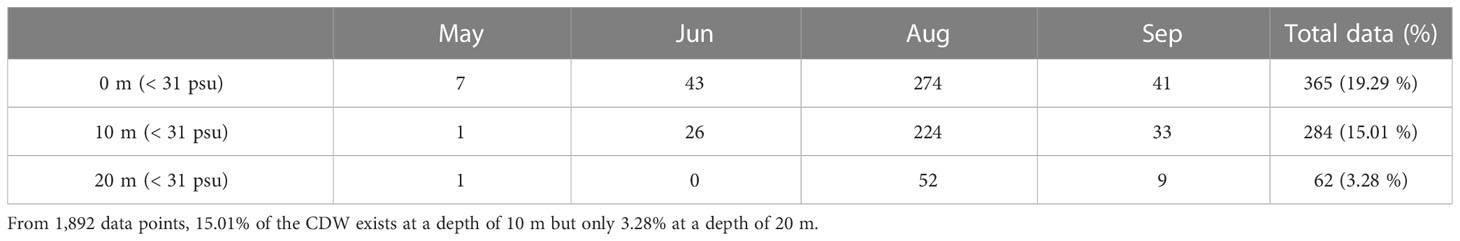
Table 1 The number of in-situ salinity data points (< 31 psu) at three depths (0, 10, and 20 m) obtained from the National Institute of Fisheries Science (NIFS) from 2015 to 2021.

Figure 1 shows the location of each station used for this study. Other validation datasets for S_10m were collected from the Ieodo Ocean Research Station (I-ORS) and the Korea Meteorological Administration (KMA). The geographical location of the I-ORS (32.07° N, 125.10° E) makes it an ideal observation site for monitoring the expansion of low salinity water from the Changjiang River. The I-ORS estimates salinity at various depths, including 10 m. Therefore, we used the I-ORS S_10m from 2020 to validate the model performance. The KMA provided CTD observation data around the Yellow Sea and ECS. Since that area plays an important role in meteorology and climatology, serial observations using shipboard were conducted every two months since January 2016 to observe changes in the marine environment; thus, we used summertime data (May to September) from 2016 to 2021. The observation point was selected to monitor the influence of the Yellow Sea Bottom Cold Water and CDW.

FIGURE 1

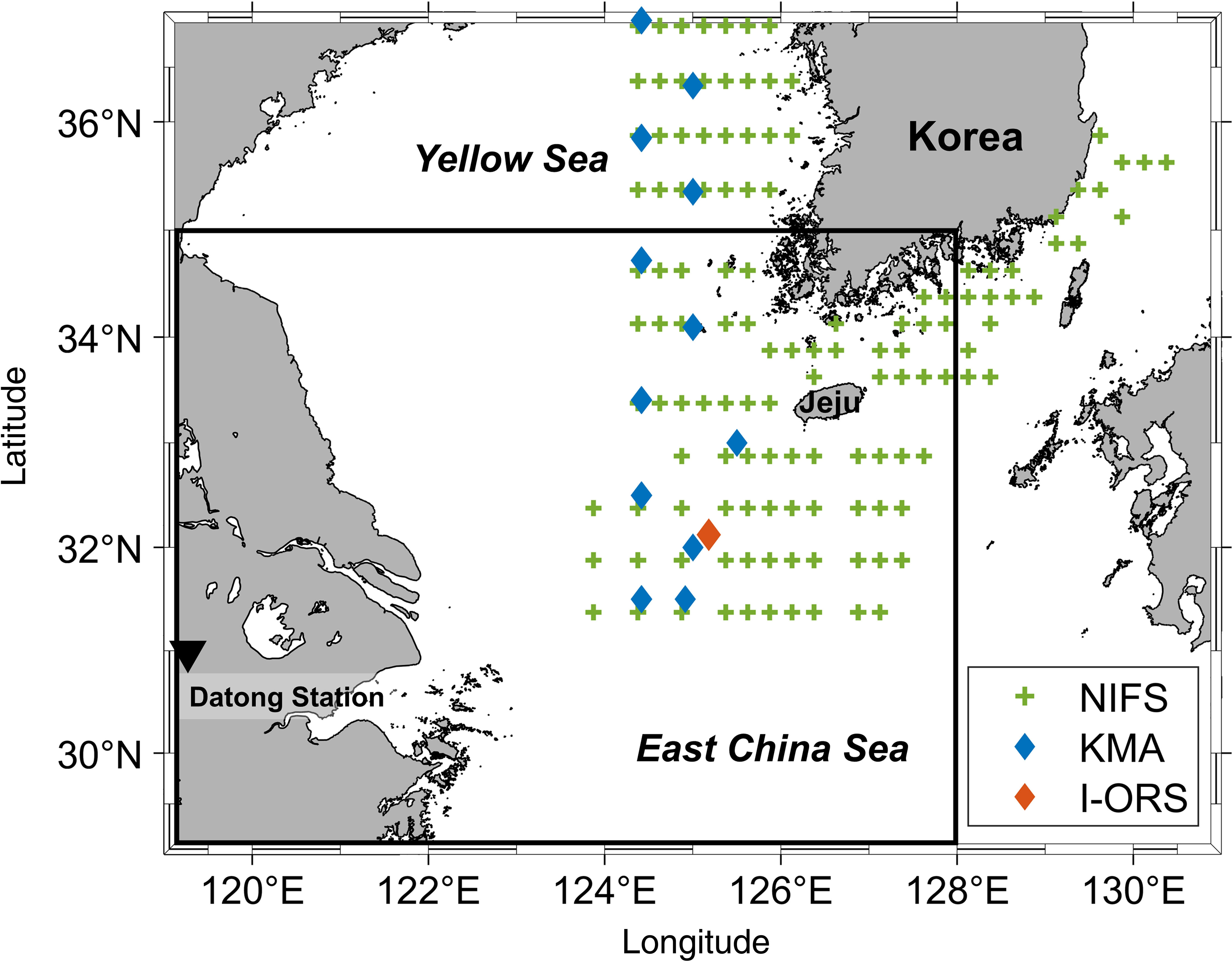
Figure 1 Study area and matching stations for the in-situ and satellite data from 2015 to 2021. The serial shipboard observation stations from National Institute of Fisheries Science (NIFS) are marked by a green cross sign. The blue and red diamonds indicate the CTD location of Korea Meteorological Administration (KMA), and Ieodo Ocean Research Station (I-ORS) used for the model validation. The black solid box is the region where the CDW volume is calculated in Section 3.

In addition, to investigate the effect of Changjiang River discharge (CRD) on CDW volume, the daily flow rate of the Changjiang River, measured by the Datong Station, was collected from 2015 to 2021 (www.cjh.com.cn). The Datong station is approximately 624 km from the Changjiang River Estuary. It is the first hydrometric station in the mainstream of the Changjiang River to the estuary and the uppermost boundary of the ocean tide. The discharge at the Datong hydrometric station generally represents the CRD streaming down to the ECS (Erfeng et al., 2003). Table 2 summarizes the datasets used in this study.

TABLE 2

Table 2 Summary of the data used in this study.

2.2 Method

To estimate the CDW volume, a CNN model was trained using a combination of satellite and in-situ data. The model was utilized to predict the salinity depth at S_10m, a proxy for CDW volume. The contributions of each input variable to the S_10m were evaluated using SHAP analysis. The distribution maps of S_10m were created for the entire study period. Based on these maps and SMAP SSS, the volume of CDW was calculated. This approach allowed for a comprehensive assessment of CDW volume using a combination of the CNN model and satellite observations.

2.2.1 Convolution neural network

In this study, we developed a CNN model to estimate the S_10m. The CNN method has been demonstrated to be superior to other deep learning methods in remote sensing applications, owing to its ability to capture spatial feature information and achieve high accuracy in spatial distribution (Yamashita et al., 2018; Meng et al, 2021a; Zuo et al., 2021; Shin et al., 2022). We constructed a CNN structure for feature extraction with one input layer, three convolution layers, three max pooling layers, three dropout layers, and one regression layer as the output layer. Rectified linear unit (ReLU) layers were used as activation functions (Figure 2).

FIGURE 2

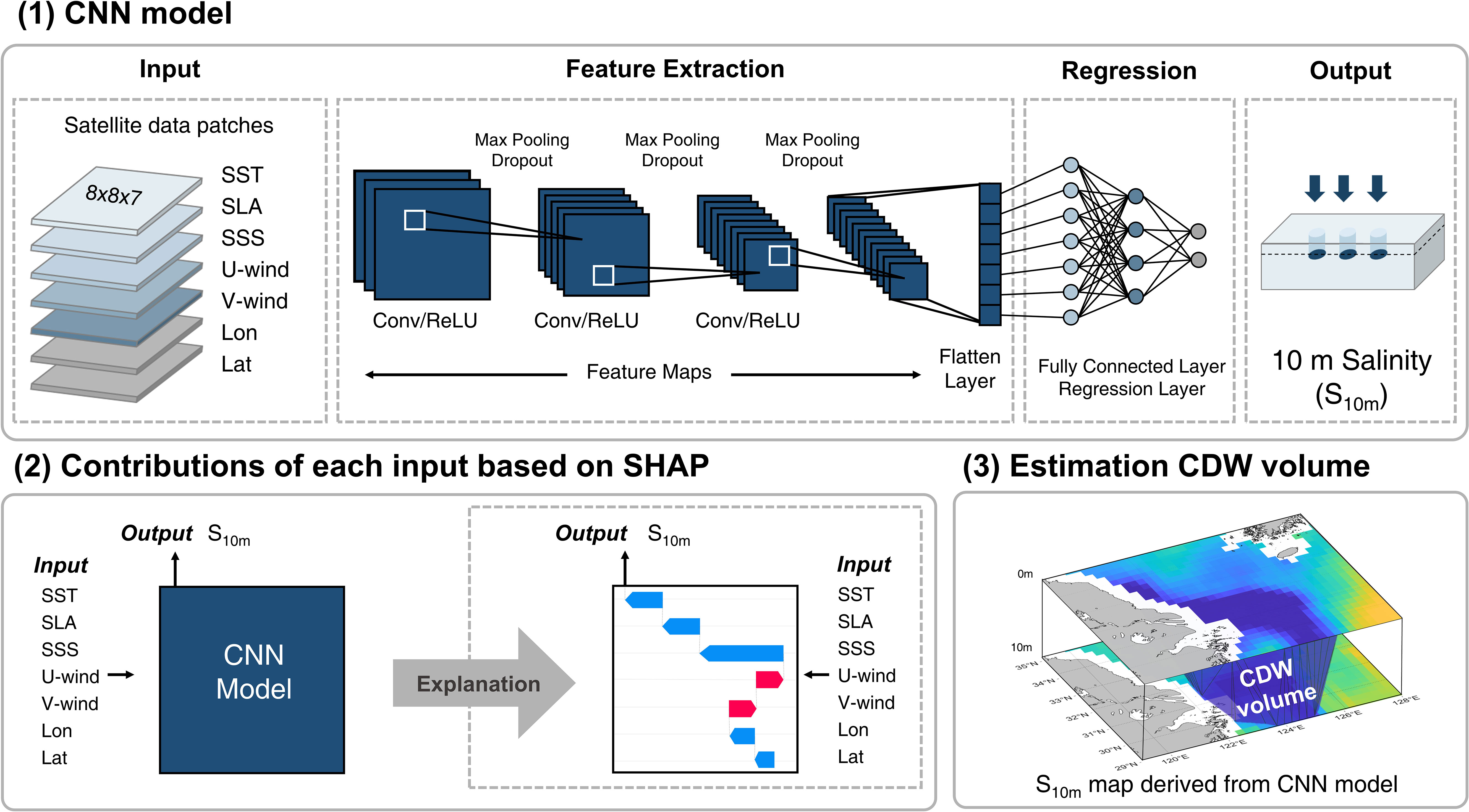
Figure 2 Schematic diagram of a convolutional neural network (CNN) model, Shapley Additive exPlanations (SHAP) analysis and CDW volume estimation. There are three steps: (1) developing a CNN architecture for estimating salinity at a depth of 10 m (S_10m), (2) conducting SHAP analysis to investigate the importance of input parameters and their interactions, and (3) calculating CDW volume based on S_10m maps generated by the CNN.

For the training dataset of CNN model, we generated patch pairs between sea surface parameters and geographical factors (latitude and longitude) as input and the corresponding in-situ S_10m as the ground truth data. Each patch was generated with a size of 8 × 8 × 7 pixels utilizing the nearest pixels of the satellite gridded dataset (25 km at daily) extracted from the corresponding in-situ salinity. Patches that did not fill at least half of the 8 × 8 pixels were excluded from the training set. The z-score standardization method was applied to process the sea surface data to weight all variables equally. A total of 1,310 coupled patches of in-situ salinity and multi-satellite data were randomly divided into two groups for training and test. The proportions of patch pairs for the training and the validation were 70 and 30%, respectively. Additionally, in-situ data sources (i.e., I-ORS and KMA) were used to evaluate the effects of different data sources on model performance. We evaluated the performance of the CNN model with in-situ salinity using various statistical values such as the determined coefficient (R²), root mean square error (RMSE), and relative RMSE (RRMSE).

2.2.2 Contributions of each input based on SHAP

We used the SHAP method to investigate the contribution between sea surface parameters and S_10m. The SHAP is one of the eXplainable Artificial Intelligence (XAI) methods developed to interpret complex black-box, artificial intelligence models. The SHAP values quantify the impact of each input feature on the model output, explaining the individual predictions of how much each input contributes to the prediction. It has the advantage of providing not only the relative importance of each input variable but also the positive or negative relationship on the output (Lundberg and Lee, 2017; Mangalathu et al., 2020; Tian et al., 2022). SHAP has been widely used in machine learning in marine science to interpret nonlinear or indirect relationships between input and output variables. It also helpful for examining complex interactions between multiple variables in such systems (Jang et al., 2021; Jang et al., 2022; Tian et al., 2022). The SHAP value was calculated using the following equation (Eq. 1):

$\begin{array}{ll}SHA{P}_i={\sum }_{z\in N\left\{i\right\}}\frac{\left|z\right|!(M-\left|z\right|-1)!}{M!} [f_{z{\cup }^{ }\left\{i\right\}}(x_{z{\cup }^{ }\left\{i\right\}})-f_z(x_z)]& (1)\end{array}$

where z indicates the subset of input parameters, N is all input parameters, M is the number of input parameters, $f_{z{\cup }^{ }\left\{i\right\}}(x_{z{\cup }^{ }\left\{i\right\}})$ is output with i^th parameter, and $f_z(x_z)$ is output without i^th parameter (Lundberg and Lee, 2017; Mangalathu et al., 2020; Jang et al., 2021). We can better understand the relationships between input and output by comparing the SHAP value for each input.

2.2.3 Estimation of CDW volume

The CDW volume (V_CDW) was calculated using Eq. 2:

$\begin{array}{ll}{V}_{CDW }=\underset{d}{\overset{0}{\int }}A(z)dz,& (2)\end{array}$

where d is the depth (here d = 10 m), A(z) is CDW area (defined as< 31 psu). We used SMAP data for the A(0) and the results of the CNN model for the A(10). The density-based spatial clustering of applications with noise (DBSCAN) method was used to isolate the area (A(z)) of CDW in gridded data. DBSCAN is a data clustering algorithm that determines the noise points or outliers and detects dense spatial points (Ester et al., 1996). We applied this method to remove outliers and extract the A(z) at each depth. To calculate the V_CDW, we used the alpha shape method, a computational geometry algorithm that creates a bounding area or volume around a given set of points (Edelsbrunner and Mücke, 1994). Since the Changjiang River plume spreads eastwards over the broad area of the ECS, reaching as far as Jeju Island, we estimated the V_CDW over a limited area affected by CDW (119–128°E, 29–35°N).

3 Results

3.1 Performance of CNN model

Figure 3 shows the performance comparison of the CNN model using various datasets. Figures 3A and B show the training and test results, respectively. In the case of the test results, the R², RMSE, and RRMSE were 0.81, 0.63 psu, and 2.00%, respectively. To validate the model results based on different data sources, we utilized in-situ data from KMA and I-ORS. The locations of each station are shown in Figure 1. Using KMA data with 181 matched datasets, the validation results showed a good level with an R², RMSE, and RRMSE of 0.65, 0.65 psu, and 2.06%, respectively (Figure 3C). We determined that the model performed well with an RMSE of< 1 psu. Figure 3D compares daily values measured by I-ORS between May and September 2020. The R², RMSE, and RRMSE was 0.80, 0.82 psu, and 2.64%, respectively. Since there were insufficient data points below 31 psu, errors were often present within this range, but overall results showed good performance with an RMSE below 1 psu. In addition, we compared the CNN results, HYCOM, and CMEMS with KMA in-situ data observed from 2016 to 2019. It was found that HYCOM tended to overestimate S_10m with an R², RMSE, and RRMSE of 0.11, 1.68 psu, and 5.10%. Similarly, CMEMS also showed low accuracy with an R², RMSE, and RRMSE of 0.23, 1.48 psu, and 4.71%. In contrast, the CNN model developed in this study demonstrated high accuracy with an R², RMSE, and RRMSE of 0.68, 0.71 psu, and 2.26%.

FIGURE 3

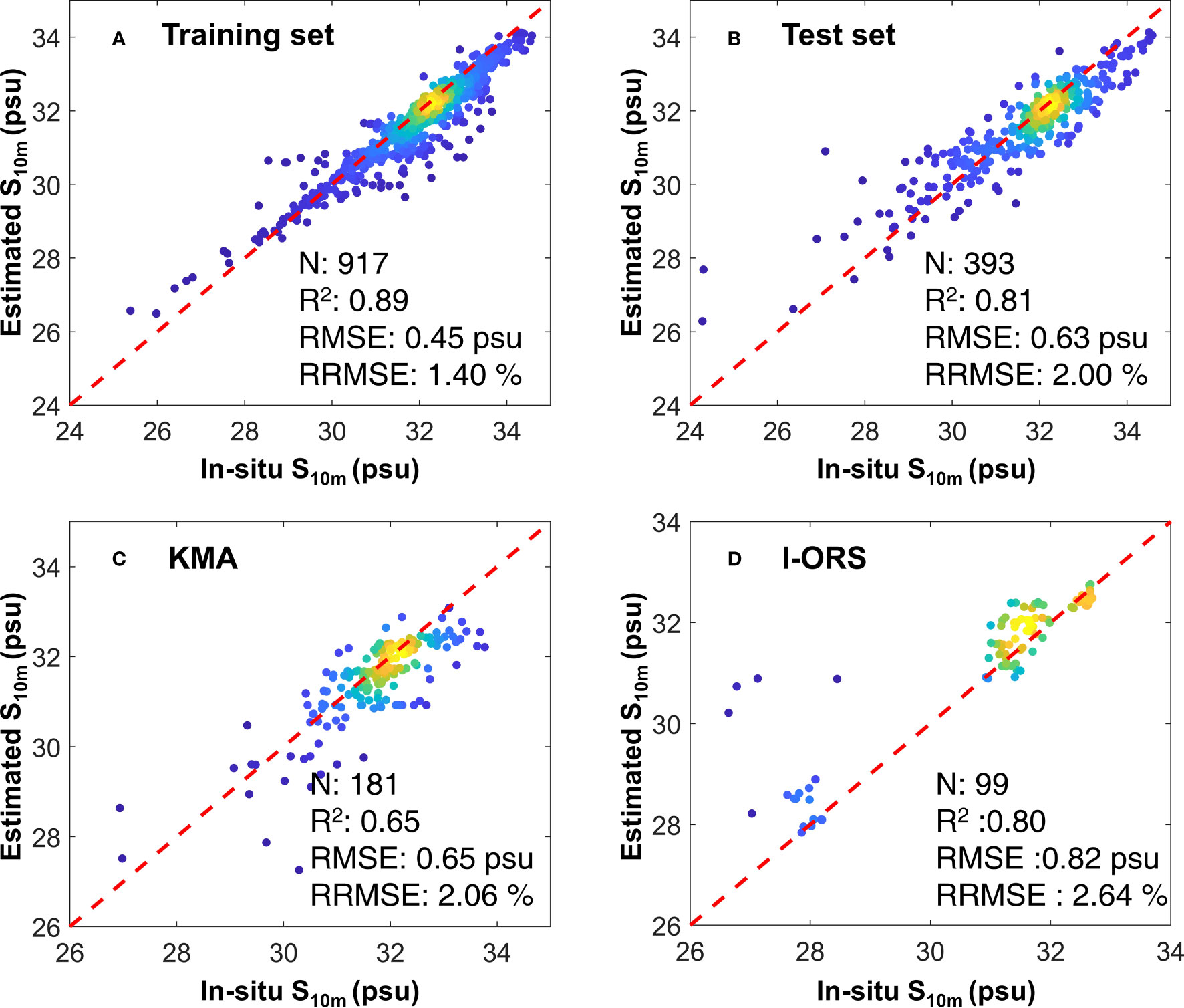
Figure 3 Density scatter plots between in-situ and estimated S_10m derived from CNN. (A, B) are the results of training and test sets, respectively. (C, D) represent the results using KMA and I-ORS data, respectively.

Figure 4 shows monthly spatial distributions of SMAP SSS, CNN result of S_10m, and ΔS (SSS–S_10m) from 2015 to 2021. The solid black and red lines represent the 31 psu isohalines at the surface and at a depth of 10 m, respectively. The CDW represents in the center of the ECS and mainly transported eastward and northeastward. The SSS showed that an increase in CDW area over time and particularly extremely low salinity values (< 28 psu) always existed near the coastal region during the summer (Figure 4A). However, S_10m was generally higher than the sea surface, and the areas with salinity below 31 psu were narrower than SSS (Figure 4B). Another significant finding was that, unlike SSS, relatively low salinity was present in the center of the ECS rather than in the coastal areas. Because of tidal mixing, low salinity was not observed near the coastal area at a depth of 10 m (Moon et al., 2009; Yu et al., 2020). The ΔS represents the difference in salinity, with a maximum difference of –2.59 psu in May and a minimum difference of –1.08 psu in September (Figure 4C). The red shaded areas indicate regions where both SSS and S_10m have a salinity of ≤ 31 psu, indicating the presence of CDW at depths greater than 10 m and its movement towards Jeju Island over time. It confirms the difference in the spatial distribution of CDW between sea surface and a depth of 10 m.

FIGURE 4

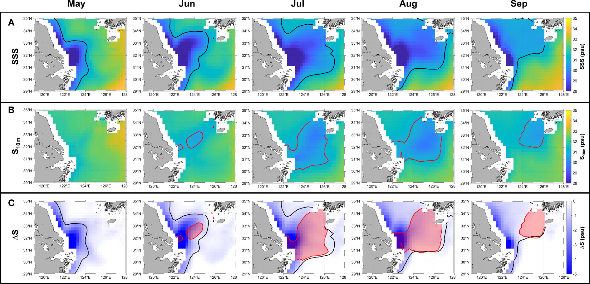
Figure 4 The monthly spatial distributions (A) SMAP SSS (B) CNN result of S_10m and (C) ΔS (SSS–S_10m) from 2015 to 2021. The solid black lines and red lines represent the 31 psu isohalines at the surface and at a depth of 10 m, respectively. Red shading indicates location where CDW exists deeper than 10 m.

3.2 Contribution of sea surface physical factors to S_10m

Using the SHAP approach, the effect of input on the output can be quantified. By comparing the SHAP values, the contribution of each input toward the output can be evaluated. Figure 5 shows the contribution of input variables affecting S_10m. The SSS was the highest at 48.42%, followed by SLA, latitude, SST, longitude, V-wind, U-wind at 13.22, 10.59, 9.31, 8.08, 5.48, and 4.90%, respectively. A negative value on the x-axis (SHAP value) indicates that the model predicts a relatively low S_10m, whereas a positive value indicates the opposite. The SSS was the most influential factor as it directly affects the S_10m and has a strong positive relationship with it. The second most important variable was SLA, which changes according to water mass and thermal expansion (Cabanes et al., 2001; Kuang et al., 2017). During the summer in the ECS, the discharge of the Changjiang River leads to an increase in water mass, which can be reflected in SLA. At the same time, the strengthening of stratification causes an increase in SST simultaneously (Park et al., 2011; Moon et al., 2019; Gao et al., 2020; Hong et al., 2022; Kim et al., 2022). Therefore, there was an inverse relation between SLA and S_10m due to low salinity in mass changes. The SSW is critical for north-eastward CDW transport because of the Ekman flow (Chang and Isobe, 2003; Siswanto et al., 2008; Moon et al., 2010). However, when predicting the S_10m, it did not show a clear relationship and had a very low contribution compared to other variables (< 6%). The SSW has a significant impact on the CDW extension but not on salinity. Hence, the SHAP analysis results suggested that the CNN model considers more realistic physical relationships between each input variable and S_10m.

FIGURE 5

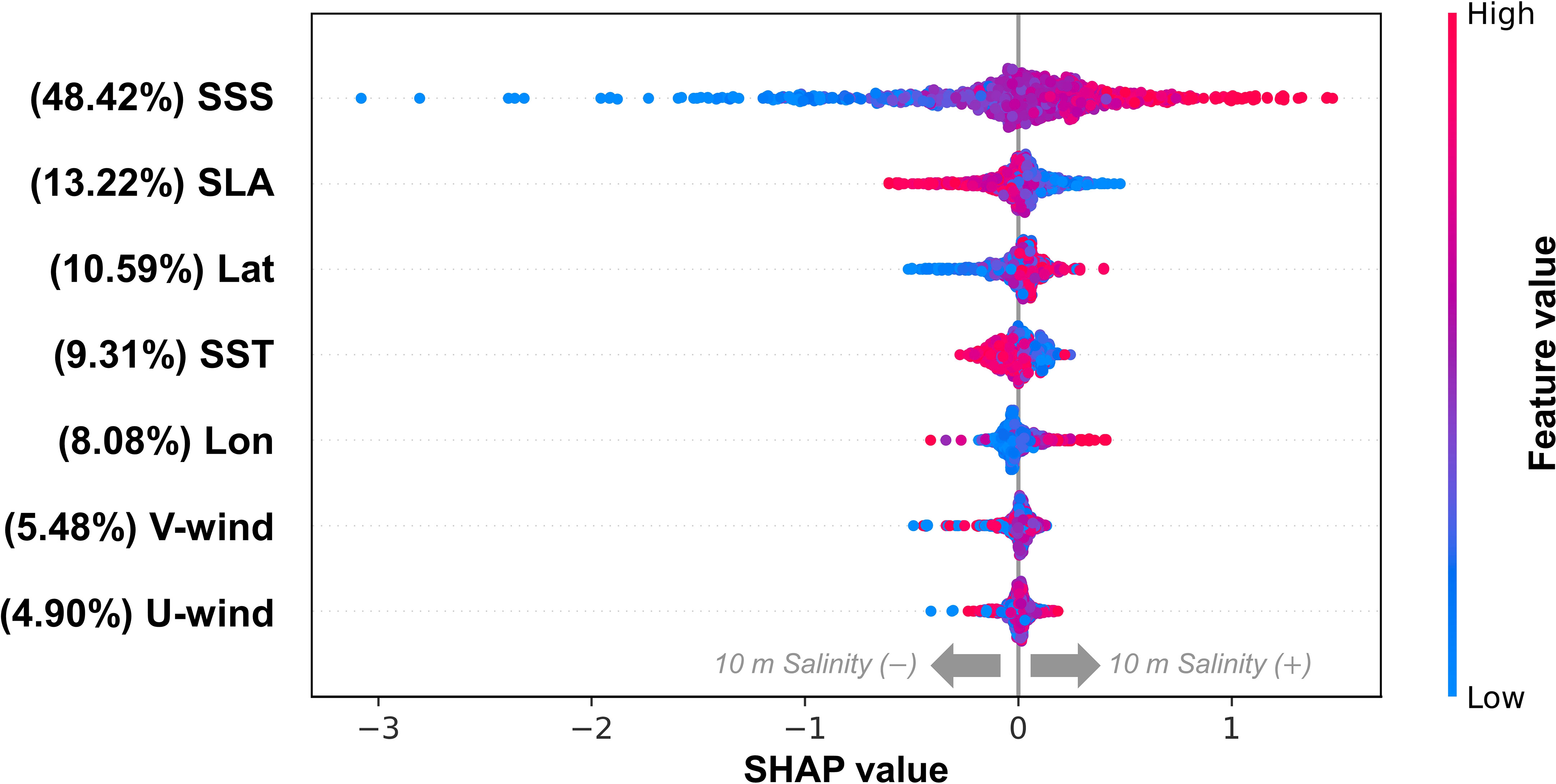
Figure 5 The summary plot of SHAP values for the CNN model. The x-axis indicates the impact of each feature to the model. The points are distributed horizontally along the x-axis according to their SHAP value. The color of dots is the value of each input variable, from low (blue) to high (red). Input variables with larger contribution are placed in ascending order.

3.3 Variation of the CDW volume

The CDW volume was calculated by combining the S_10m map obtained from CNN with the SMAP SSS. It was created daily during the summer (May to September) from 2015 to 2021 (Figure 6A). When compared annually, the CDW volume was highest in 2016 (3.01×10¹² m³), followed by 2020 (2.46×10¹² m³) and 2015 (2.32×10¹² m³). However, in 2018, the CDW reached a minimum volume (1.31×10¹² m³). The CDW volume showed a seasonal trend, with relatively low values from May to early June and an increasing trend from June to August (Figure 6B). The lowest value was recorded in May at approximately 0.30×10¹² m³, while the highest was in August at 1.74×10¹² m³ and then decreased to 1.05×10¹² m³ in September. On average, there is a variation of 1.44×10¹²m³ in CDW volume during the summer season.

FIGURE 6

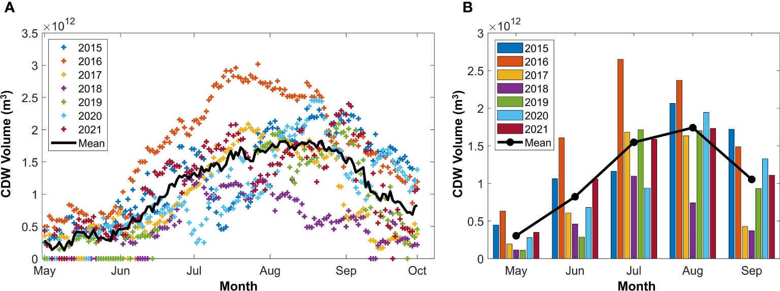
Figure 6 Time series of (A) daily and (B) monthly CDW volumes from 2015 to 2021. The black line indicates the annual mean value.

We investigated the spatial distribution of CDW volume at a depth of 10 m. Figure 7 shows the percentage of pixels included when calculating the volume of CDW that exists at depths of ≥ 10 m. The percentage represents the frequency of the pixels that were used to calculate the volume at 10 m each month. For example, pixels indicating 100% represent the presence of CDW at depths ≥ 10 m throughout the month in the corresponding locations. Figures 7A, B show the pixels for 2016 and 2018, which recorded the highest and lowest CDW volumes, respectively. In 2016, when the volume was more extensive, it was observed that CDW existed at depths > 10 m and gradually moved towards the Jeju coast over time. CDW in July spread extensively in the ECS throughout the month. In contrast, CDW in 2018 was located in a relatively narrow area. The spatial distribution of CDW at a depth of 10 m varied significantly depending on the volume.

FIGURE 7

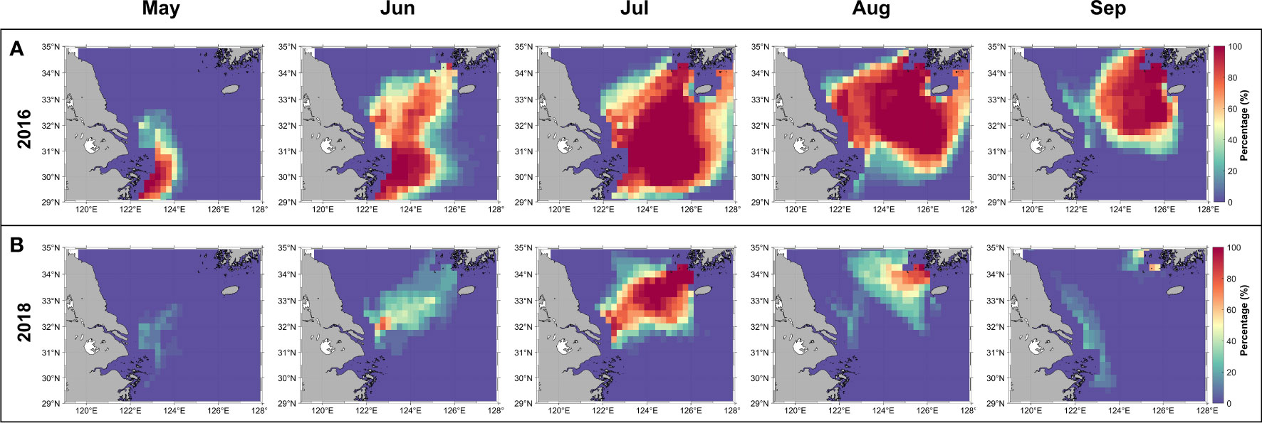
Figure 7 Percentage of pixels included in the volume calculation by month, where CDW exists in deeper than 10 m. (A) The maximum volume in 2016 and (B) the minimum volume in 2018. A value of 100% indicates that CDW is always present in the area during the month.

3.4 Sea surface warming caused by different CDW volume

To investigate the impact of CDW on SST, we compared S_10m values and sea surface temperature anomaly (SSTA) in 2016 and 2018, when the CDW volume was at its maximum (3.01 × 10¹² m³) and minimum (1.31 × 10¹² m³), respectively. Figures 8A, D depict the time series of ΔS (SSS–S_10m) and SSTA from I-ORS. The ΔS represents the difference in between surface salinity and S_10m, demonstrating the degree of stratification caused by salinity. The black box denotes the period corresponding to CDW, which persisted for 117 days in 2016. Throughout this period, ΔS consistently indicated negative values, indicating the presence of salinity stratification induced by CDW. Consequently, there was an overall increase of 4.79 °C in SSTA. These findings support the conclusion by Moon et al. (2019) that strong stratification caused by low salinity water significantly increases SST. In contrast, in 2018, the influence of CDW continued for 44 days and increased SSTA by 2.19 °C (Figure 8D). The low increase in SSTA observed in 2018 compared to 2016 can be attributed to a decrease in the CDW volume, leading to a shorter period of low salinity effects. The spatial distribution of ΔS and SSTA are shown in Figures 8B, C, respectively. During 2016, the low values of ΔS indicated strong stratification caused by salinity, particularly in the center of the ECS (yellow lines). The distribution of SSTA also showed high values in areas adjacent to regions with low ΔS values, and it corresponds to the CTD observation results reported by Moon et al. (2019). It is possible that CDW contributed to the increase in SST, as suggested by previous studies (Park et al., 2011; Moon et al., 2019; Gao et al., 2020; Park et al., 2020; Hong et al., 2022). However, ΔS was mostly zero in 2018, suggesting a well-mixed condition, and SSTA showed low values (Figures 8E, F). Unlike in 2016, there was no clear relationship between salinity and SSTA.

FIGURE 8

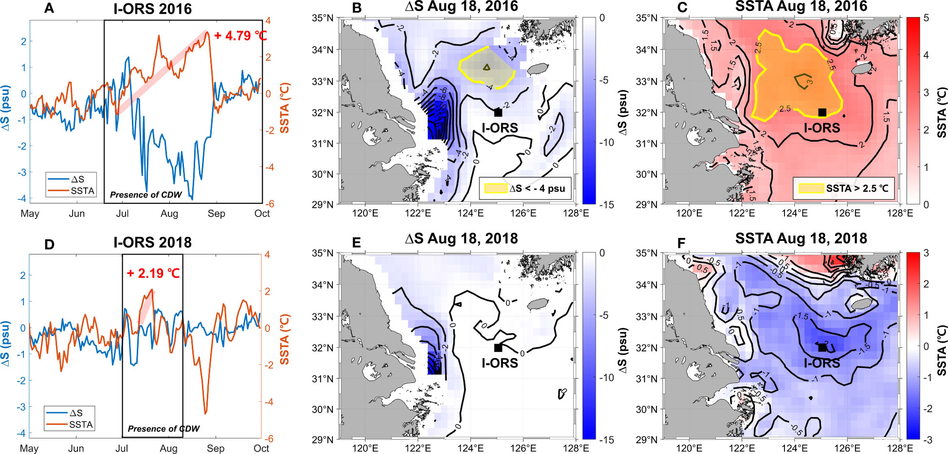
Figure 8 Time series of ΔS (SSS–S_10m) and SSTA from I-ORS in (A) 2016 and (D) 2018, respectively. The black box represents the length of time CDW has existed. (B, C) are the spatial distribution of ΔS and SSTA on August 18, 2016, respectively, while (E, F) show the same for August 18, 2018.

4 Discussion

4.1 Importance of geographical factors

We selected physically related variables and geographic information as input factors to estimate the S_10m as sea surface parameters. To investigate the importance of geographic information, we compared the results of the model trained with only physical factors with the model with geographic information included. The results showed that the model without geographic information had lower accuracy, with an R², RMSE, and RRMSE of 0.79, 0.67 psu, and 2.13%, respectively, in the test set compared to the model with geographic information included. The SHAP analysis applied to this model revealed that the contribution of each variable was as follows: SSS (56.36%), SLA (17.07%), SST (12.67%), V-wind (7.48%), and U-wind (6.42%). When geographical information was excluded, the relative importance of other variables increased, but the order of variable importance remained the same (Figure 5). The geographical information represents the significance of the Changjiang River location in this study. The Changjiang River is a dominant source of freshwater in the ECS and is located southwest of our study area. As the latitude and longitude decrease (blue), it gets closer to the mouth of the Changjiang River, resulting in low S_10m values. In addition, the results suggest that latitude has a more significant impact than longitude. The CDW from the Changjiang River tends to spread eastward and therefore exists over a relatively wide range of longitudes (Figure 4). Therefore, changes in latitude have a more significant effect on S_10m changes than that in longitude. It allows us to recognize that physical and geographical factors both have a significant impact on model performance.

4.2 Additional environmental factors

In addition to physical surface parameters used as input data, there are other environmental factors that can influence the volume of CDW. The primary factors responsible for decreasing the salinity of seawater are river inflows and precipitation. In particular, the ECS is highly affected by the Changjiang River, monsoon systems, and typhoons in the summer (Beardsley et al., 1985; Chen et al., 1994; Chang and Isobe, 2003; Lie et al., 2003; Kim et al., 2009; Son et al., 2020; Hong et al., 2022; Jung et al., 2022). Therefore, we addressed the CDW volume changes due to the influence of CRD and precipitation, which directly increases the freshwater in the ocean. Furthermore, we analyzed the impact of Typhoon Bavi (occurred in 2020).

4.2.1 Relationship between CRD and CDW volume

We analyzed the relationship between the CDW volume and CRD, which is the main controlling factor for CDW (Figure 9) (Beardsley et al., 1985; Lie et al., 2003; Chen et al., 2008; Siswanto et al., 2008). In spring (May to early June), the CDW volume was close to zero and peaked in July as the CRD increased. It should be noted that there was a time lag of 34 ± 15 days between the CDW volume and CRD. This is consistent with previous studies demonstrating that the CDW extends eastward in June with increasing CRD and reaches Jeju Island after 1–2 months (Chen et al., 2008; Kim et al., 2009; Son and Choi, 2022). Moreover, the years with the maximum volume in July (2016, 2017, 2018, and 2019) had an average time lag of 24.3 days, while the years with the maximum volume in August (2015, 2020, and 2021) had a longer time lag of 46.3 days. It does seem to depend on different mechanisms affecting the movement of CDW, such as wind and ocean currents. Particularly in 2021, CRD appeared to be different from other years, and it seemed to be artificially adjusted. It can be occurred by the impact of the Three Gorge Dam.

FIGURE 9

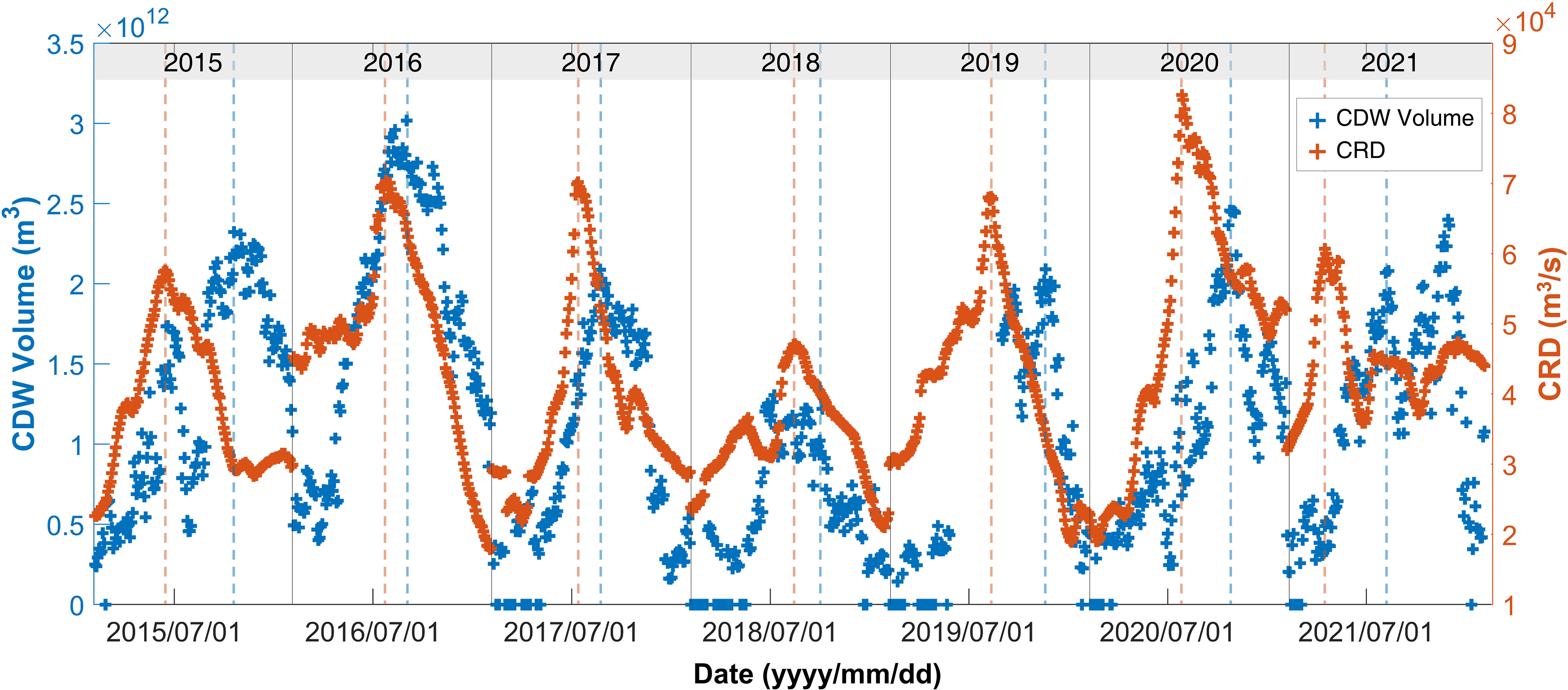
Figure 9 Time series of CDW volume and Changjiang River discharge (CRD) from 2015 to 2021. The blue dashed lines are peaks of CDW volume, and the orange dashed lines are peaks of CRD.

4.2.2 Effects of freshwater inflow by CRD and precipitation

We conducted a comparison between the monthly cumulative sum of CRD (Q_CRD) and the monthly average volume to examine the variation in CDW volume with respect to the inflow of CDW (Table 3). Q_CRD revealed an increasing trend and reached its maximum (9.73×10¹⁰ m³) in July and then decreased from August. With a 1,000-times difference in units between CDW volume and Q_CRD, we converted the values into a range between 0 and 1 using minimum-maximum (min-max) scaling and conducted regression analysis. Figure 10A displays the scatter plot for the entire period. It was observed that CDW volume and CRD have a positive correlation (Beardsley et al., 1985; Lie et al., 2003; Chen et al., 2008; Siswanto et al., 2008; Bai et al., 2014). We conducted the monthly regression coefficients to compare the impact of each month (Figure 10B). The influence of Q_CRD on volume increased over time, with a maximum impact (1.32) in August. This may be due to the one-month time lag from when CRD reached its maximum in July to the study area. It suggested that the rapid decrease in Q_CRD after July contributed significantly to the decrease in CDW volume after August.

TABLE 3

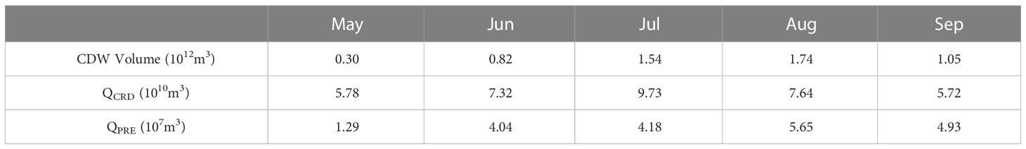
Table 3 Monthly CDW volume, accumulated CRD (Q_CRD), and accumulated precipitation (Q_PRE) from 2015 to 2021.

FIGURE 10

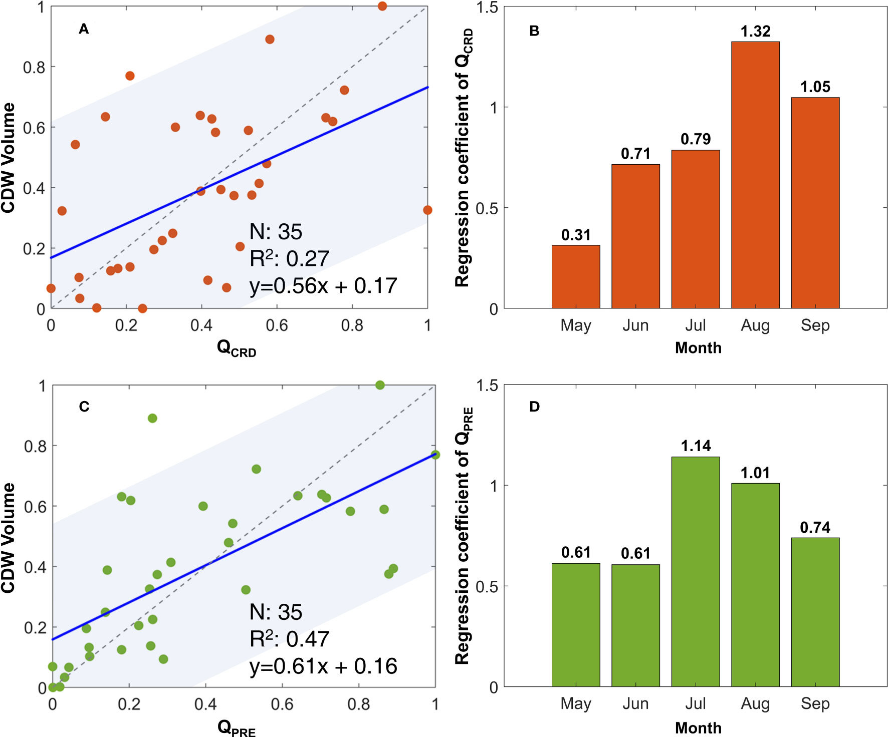
Figure 10 Scatter plot between CDW volume (A) Q_CRD and (C) Q_PRE from 2015 to 2021. Blue line is slope of each variable and blue shading indicates 95% confidence levels. Monthly regression coefficient of (B) Q_CRD and (D) Q_PRE. All values are normalized to be between 0 and 1. P-value is less than 0.05, the regression is significant.

Another factor, precipitation was calculated using Eq. 3:

$\begin{array}{ll}{Q}_{PRE}={\displaystyle \sum A\times P}& (3)\end{array}$

where A is CDW area, which is the region with SSS< 31 psu, and P represents the precipitation that falls in area A. Precipitation immediately enters the ocean; thus, the inflow of precipitation to the CDW area was calculated as the monthly cumulative sum of precipitation (Q_PRE). As shown in Table 3, the highest values of Q_PRE were observed in August (5.65×10⁷ m³) which can be attributed to heavy precipitation caused by typhoons. During the entire study period, 12 typhoons passed through the area, and 10 of them occurred in August and September (reported by KMA). To investigate the influence of Q_PRE on volume fluctuations, we applied min-max scaling and conducted a regression analysis (Figure 10C). In Figure 10D, the monthly contribution was highest in July, with a coefficient of 1.14, followed by August, with 1.01. From the results, it is clear that the precipitation, particularly during the monsoon season, significantly affects CDW volume fluctuations.

In summary, while the monthly trends showed a one-month time lag between CRD and CDW volume changes, precipitation had a more immediate effect on CDW volume due to its direct entry into the ocean (Table 3). Regression analysis determined the extent to which each factor affected CDW volume. By comparing monthly regression coefficients, the CRD had the most significant influence in August, while precipitation had the greatest impact in July. These results demonstrated that the influence of CRD and precipitation on CDW volume variation differs from month to month. Furthermore, the Q_CRD was 1,000 times larger than the Q_PRE. However, the study only measured precipitation within the CDW region and did not consider horizontal dispersion, which may have led to an underestimation of the influence of freshwater input. To obtain a more comprehensive understanding, further investigation into the impact of freshwater input and additional factors is required.

4.2.3 Effects of typhoon on CDW volume changes in 2020

When the highest CRD was recorded in 2020, we compared the I-ORS S_10m with the CNN S_10m (Figure 11A). The variation patterns of S_10m (blue lines) were similar for the entire period, and a rapid decrease in S_10m occurred in August 2020 due to a large amount of freshwater flowing into the ECS. It was confirmed that the CDW volume (orange line) also increased accordingly. To identify the effect of CDW near the I-ORS, the S_10m spatial distributions were generated before the salinity decrease, during the intrusion of CDW, and after salinity recovery following Typhoon Bavi (Figures 11B–D). During August 24–26 (shown as gray shading in Figure 11A), Typhoon Bavi moved northward and passed through near the I-ORS as a super typhoon with a strong wind speed (maximum of 66.1 m/s reported by the KMA). A rapid increase in salinity occurred in SSS (8 psu reported by KMA) and S_10m (2.61 psu) after the typhoon passed on August 26. Regarding CDW volume, an extreme decrease (0.77×10¹² m³) occurred during the same period. This result demonstrated that extreme vertical mixing induced by the typhoon as reported by Hong et al. (2022). In addition, it should be noted that CDW was eliminated and divided into two patches along the typhoon track (Figure 11D). Lee et al. (2017) suggested that the impact of typhoons inhibited the spread of CDW and induced vertical mixing, preventing its persistence. Therefore, although the CRD was highest in 2020, the relatively small CDW volume compared to 2016 (Figure 9) could be due to the dissipation of CDW caused by the typhoon.

FIGURE 11

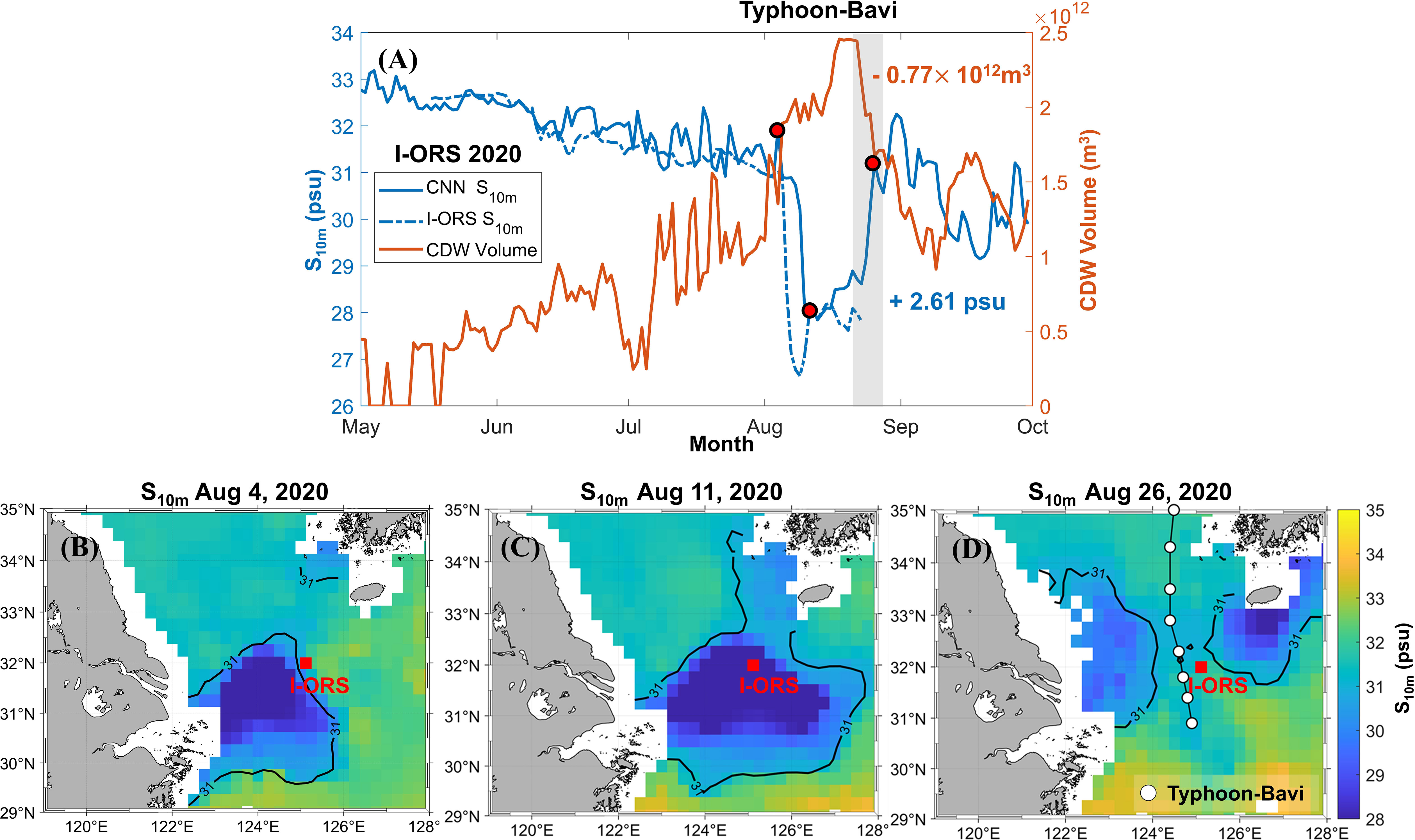
Figure 11 (A) Time series of CNN S_10m, I-ORS S_10m, and CDW volume from May to September 2020. The blue solid line indicates S_10m derived from the CNN model and the blue dashed line is the in-situ S_10m from I-ORS. The orange line shows the CDW volume of the entire study area. (B-D) Spatial distributions of each date of red circles in (A); black lines are 31 psu isohalines. (D) White dots are tracks of Typhoon Bavi (reported by the KMA).

4.3 Different ocean conditions in 2016 and 2018

The difference in ocean conditions between 2016 and 2018 may be attributed to various climatological effects, including ENSO, typhoons, and wind. The ENSO can increase the CRD by increasing precipitation during El Niño in the ECS (Park et al., 2011; Park et al., 2015; Wu et al., 2023). Typhoons are frequent oceanic events during summer in the ECS and are often accompanied by strong precipitation and winds. The strong vertical mixing caused by the passage of a typhoon hinders the expansion of CDW (Lee et al., 2017; Hong et al., 2022; Jung et al., 2022). Wind also plays a role by inducing CDW movement and vertical mixing. Therefore, we examined the oceanic environment conditions during 2016 and 2018, which exhibited significant differences in SSTA due to variations in the CDW volume. In 2016, a strong El Niño event led to a noticeable increase in CRD compared to other years (Figure 9). The increased CRD contributed to an increase in CDW volume, which significantly decreased salinity in the ECS. According to the KMA best track, no typhoons were passing through the ECS from May to September 2016, meaning there was no vertical mixing caused by typhoons. Therefore, these factors likely prolonged the persistence of CDW, resulting in higher SSTA compared to other years (Figures 8B, C). In contrast to 2016, 2018 had a low CDW volume due to low CRD caused by La Niña (Figure 9). In 2018, three typhoons, Ampil, Rumbia, and Soulik, passed through the ECS (reported KMA), which may have caused frequent vertical mixing and hindered the persistence of CDW. According to Gao et al (2020) there were strong winds in 2018, causing more wind-induced vertical mixing than in 2016.

Our analysis showed that in 2016, the increase in CRD resulted in a significant increase in CDW volume. The absence of typhoons and weak winds allowed CDW to have a persistent influence, resulting in high SSTA. In contrast, in 2018, a low SSTA was observed due to a decrease in CRD and frequent typhoons, as well as strong winds causing vertical mixing. The summer marine environment in the ECS is influenced by various factors. Therefore, to better understand the impact of CDW, it is crucial to consider these factors together.

5 Conclusions

The summer marine environment of the ECS is influenced by CDW volume. In this study, we estimated CDW volume and investigated its spatial and temporal variation. The main findings are as follows:

(1) The CNN model generated S_10m using sea surface parameters, including SST, SLA, SSW, SSS, longitude, and latitude. It had a high accuracy with R², RMSE, and RRMSE values of 0.81, 0.63 psu, and, 2.00%, respectively. Additionally, the validation results with KMA and I-ORS showed an RMSE of< 1 psu.

(2) The SHAP approach was employed to assess the impact of input variables on the model output. The analysis revealed that SSS had the highest contribution of 48.42% and a positive relationship with S_10m. The SLA followed with a contribution of 13.22% and a negative relationship, indicating that the CNN model considered more realistic physical relationships.

(3) By analyzing the temporal and spatial variation of CDW volume at a depth of 10 m, we found that the maximum volume of 3.01×10¹² m³ occurred in 2016, while the minimum volume of 1.31×10¹² m³ in 2018. Similarly, when investigating the monthly variation, the lowest volume of 0.30×10¹² m³ was recorded in May, while the highest volume of 1.74×10¹² m³ was recorded in August, followed by a decreasing trend from September.

(4) Influence of CDW on sea surface warming was compared in 2016 and 2018, when there was a significant difference in CDW volume. It shows that CDW enhanced SST for 117 days in 2016, resulting in a total increase of 4.79 °C. In contrast, CDW persisted for 44 days in 2018, resulting in a total increase of 2.19 °C. The distribution of SSTA also showed high values in areas adjacent to regions with significant differences in ΔS.

These results will greatly contribute to understanding CDW volume changes and its impact on the stratifications in the ECS. We also identified other environmental factors that influence the CDW volume, such as CRD, precipitation, and typhoons. Further research is required to investigate the detailed processes related to the CDW responses in the ECS.

Data availability statement

The original contributions presented in the study are included in the article/supplementary material. Further inquiries can be directed to the corresponding author.

Author contributions

Conceptualization: S-HK and Y-HJ. Data curation: S-HK, JS, and D-WK. Methodology: S-HK, JS, and Y-HJ. Formal analysis: S-HK, JS, D-WK, and Y-HJ. Writing-original draft: S-HK. Writing-review and editing: S-HK, JS, D-WK, and Y-HJ. All authors contributed to the article and approved the submitted version.

Funding

This study was supported by grant from the project titled “Development of technology using analysis of ocean satellite images” (20210046),(20220546) and (RS-2023-00256330) by the Korea Institute of Marine Science and Technology Promotion (KIMST), funded by the Ministry of Oceans and Fisheries.

Conflict of interest

The authors declare that the research was conducted in the absence of any commercial or financial relationships that could be construed as a potential conflict of interest.

Publisher’s note

All claims expressed in this article are solely those of the authors and do not necessarily represent those of their affiliated organizations, or those of the publisher, the editors and the reviewers. Any product that may be evaluated in this article, or claim that may be made by its manufacturer, is not guaranteed or endorsed by the publisher.

References

Bai Y., He X., Pan D., Chen C. T. A., Kang Y., Chen X., et al. (2014). Summertime Changjiang River plume variation during 1998–2010. J. Geophysical Research: Oceans 119 (9), 6238–6257. doi: 10.1002/2014JC009866

CrossRef Full Text | Google Scholar

Bao S., Zhang R., Wang H., Yan H., Yu Y., Chen J. (2019). Salinity profile estimation in the Pacific Ocean from satellite surface salinity observations. J. Atmospheric Oceanic Technol. 36 (1), 53–68. doi: 10.1175/JTECH-D-17-0226.1

CrossRef Full Text | Google Scholar

Beardsley R. C., Limeburner R., Yu H., Cannon G. A. (1985). Discharge of the Changjiang (Yangtze river) into the East China sea. Continental Shelf Res. 4 (1-2), 57–76. doi: 10.1016/0278-4343(85)90022-6

CrossRef Full Text | Google Scholar

Cabanes C., Cazenave A., Le Provost C. (2001). Sea level rise during past 40 years determined from satellite and in situ observations. Science 294 (5543), 840–842. doi: 10.1126/science.1063556

PubMed Abstract | CrossRef Full Text | Google Scholar

Chang P. H., Isobe A. (2003). A numerical study on the Changjiang diluted water in the Yellow and East China Seas. J. Geophysical Research: Oceans 108 (C9). doi: 10.1029/2002JC001749

CrossRef Full Text | Google Scholar

Chen C. T. A. (2009). Chemical and physical fronts in the Bohai, Yellow and East China seas. J. Mar. Syst. 78 (3), 394–410. doi: 10.1016/j.jmarsys.2008.11.016

CrossRef Full Text | Google Scholar

Chen C., Beardsley R. C., Limeburner R., Kim K. (1994). Comparison of winter and summer hydrographic observations in the Yellow and East China Seas and adjacent Kuroshio during 1986. Continental Shelf Res. 14 (7-8), 909–929. doi: 10.1016/0278-4343(94)90079-5

CrossRef Full Text | Google Scholar

Chen C., Xue P., Ding P., Beardsley R. C., Xu Q., Mao X., et al. (2008). Physical mechanisms for the offshore detachment of the Changjiang Diluted Water in the East China Sea. J. Geophysical Research: Oceans 113 (C2). doi: 10.1029/2006JC003994

CrossRef Full Text | Google Scholar

Dong L., Qi J., Yin B., Zhi H., Li D., Yang S., et al. (2022). Reconstruction of subsurface salinity structure in the south China sea using satellite observations: A lightGBM-based deep forest method. Remote Sens. 14 (14), 3494. doi: 10.3390/rs14143494

CrossRef Full Text | Google Scholar

Edelsbrunner H., Mücke E. P. (1994). Three-dimensional alpha shapes. ACM Trans. On Graphics (TOG) 13 (1), 43–72. doi: 10.1145/174462.156635

CrossRef Full Text | Google Scholar

Erfeng Z., Xiqing C., Xiaoli W. (2003). Water discharge changes of the Changjiang River downstream Datong during dry season. J. Geographical Sci. 13, 355–362. doi: 10.1007/BF02837511

CrossRef Full Text | Google Scholar

Ester M., Kriegel H. P., Sander J., Xu X. (1996). Density-based spatial clustering of applications with noise. In Int. Conf. knowledge Discovery Data Min. Vol. 240, 6.

Google Scholar

Gao G., Marin M., Feng M., Yin B., Yang D., Feng X., et al. (2020). Drivers of marine heatwaves in the East China Sea and the South Yellow Sea in three consecutive summers during 2016–2018. J. Geophysical Research: Oceans 125 (8), e2020JC016518. doi: 10.1029/2020JC016518

CrossRef Full Text | Google Scholar

Hong J. S., Moon J. H., Kim T., You S. H., Byun K. Y., Eom H. (2022). Role of salinity-induced barrier layer in air-sea interaction during the intensification of a typhoon. Front. Mar. Sci. 9, 235. doi: 10.3389/fmars.2022.844003

CrossRef Full Text | Google Scholar

Jang E., Kim Y. J., Im J., Park Y. G. (2021). Improvement of SMAP sea surface salinity in river-dominated oceans using machine learning approaches. GIScience Remote Sens. 58 (1), 138–160. doi: 10.1080/15481603.2021.1872228

CrossRef Full Text | Google Scholar

Jang E., Kim Y. J., Im J., Park Y. G., Sung T. (2022). Global sea surface salinity via the synergistic use of SMAP satellite and HYCOM data based on machine learning. Remote Sens. Environ. 273, 112980. doi: 10.1016/j.rse.2022.112980

CrossRef Full Text | Google Scholar

Jung Y. J., Choi B. J., Kwon K., Lee S. H. (2022). Modeling surface low-salinity pools formed by heavy precipitation in the Yellow Sea. Estuarine Coast. Shelf Sci. 275, 107987. doi: 10.1016/j.ecss.2022.107987

CrossRef Full Text | Google Scholar

Kim D. W., Kim S. H., Jo Y. H. (2022). Machine learning to identify three types of oceanic fronts associated with the changjiang diluted water in the east China sea between 1997 and 2021. Remote Sens. 14 (15), 3574. doi: 10.3390/rs14153574

CrossRef Full Text | Google Scholar

Kim H. C., Yamaguchi H., Yoo S., Zhu J., Okamura K., Kiyomoto Y., et al. (2009). Distribution of Changjiang diluted water detected by satellite chlorophyll-a and its interannual variation during 1998–2007. J. Oceanography 65, 129–135. doi: 10.1007/s10872-009-0013-0

CrossRef Full Text | Google Scholar

Klemas V., Yan X. H. (2014). Subsurface and deeper ocean remote sensing from satellites: An overview and new results. Prog. Oceanography 122, 1–9. doi: 10.1016/j.pocean.2013.11.010

CrossRef Full Text | Google Scholar

Kuang C., Chen W., Gu J., Su T. C., Song H., Ma Y., et al. (2017). River discharge contribution to sea-level rise in the Yangtze River Estuary, China. Continental Shelf Res. 134, 63–75. doi: 10.1016/j.csr.2017.01.004

CrossRef Full Text | Google Scholar

Lee J. H., Moon I. J., Moon J. H., Kim S. H., Jeong Y. Y., Koo J. H. (2017). Impact of typhoons on the C hangjiang plume extension in the Y ellow and E ast C hina S eas. J. Geophysical Research: Oceans 122 (6), 4962–4973. doi: 10.1002/2017JC012754

CrossRef Full Text | Google Scholar

Lie H. J., Cho C. H., Lee J. H., Lee S. (2003). Structure and eastward extension of the Changjiang River plume in the East China Sea. J. Geophysical Research: Oceans 108 (C3). doi: 10.1029/2001JC001194

CrossRef Full Text | Google Scholar

Lu W., Su H., Yang X., Yan X. H. (2019). Subsurface temperature estimation from remote sensing data using a clustering-neural network method. Remote Sens. Environ. 229, 213–222. doi: 10.1016/j.rse.2019.04.009

CrossRef Full Text | Google Scholar

Lundberg S. M., Lee S. I. (2017). A unified approach to interpreting model predictions. Adv. Neural Inf. Process. Syst. 30.

Google Scholar

Mangalathu S., Hwang S. H., Jeon J. S. (2020). Failure mode and effects analysis of RC members based on machine-learning-based SHapley Additive exPlanations (SHAP) approach. Eng. Structures 219, 110927. doi: 10.1016/j.engstruct.2020.110927

CrossRef Full Text | Google Scholar

Meng L., Yan X. H. (2022). “Remote Sensing for Subsurface and Deeper Oceans: An overview and a future outlook,” in IEEE geoscience and remote sensing magazine. New York, US.

Google Scholar

Meng L., Yan C., Zhuang W., Zhang W., Geng X., Yan X. H. (2021a). Reconstructing high-resolution ocean subsurface and interior temperature and salinity anoMalies from satellite observations. IEEE Trans. Geosci. Remote Sens. 60, 1–14. doi: 10.1109/TGRS.2021.3109979

CrossRef Full Text | Google Scholar

Meng L., Yan C., Zhuang W., Zhang W., Yan X. H. (2021b). Reconstruction of three-dimensional temperature and salinity fields from satellite observations. J. Geophysical Research: Oceans 126 (11), e2021JC017605. doi: 10.1029/2021JC017605

CrossRef Full Text | Google Scholar

Moon J. H., Hirose N., Yoon J. H., Pang I. C. (2010). Offshore detachment process of the low-salinity water around Changjiang Bank in the East China Sea. J. Phys. Oceanography 40 (5), 1035–1053. doi: 10.1175/2010JPO4167.1

CrossRef Full Text | Google Scholar

Moon J. H., Kim T., Son Y. B., Hong J. S., Lee J. H., Chang P. H., et al. (2019). Contribution of low-salinity water to sea surface warming of the East China Sea in the summer of 2016. Prog. Oceanography 175, 68–80. doi: 10.1016/j.pocean.2019.03.012

CrossRef Full Text | Google Scholar

Moon J. H., Pang I. C., Yoon J. H. (2009). Response of the Changjiang diluted water around Jeju Island to external forcings: A modeling study of 2002 and 2006. Continental Shelf Res. 29 (13), 1549–1564. doi: 10.1016/j.csr.2009.04.007

CrossRef Full Text | Google Scholar

Olmedo E., Taupier-Letage I., Turiel A., Alvera-Azcárate A. (2018). Improving SMOS sea surface salinity in the Western Mediterranean sea through multivariate and multifractal analysis. Remote Sens. 10 (3), 485. doi: 10.3390/rs10030485

CrossRef Full Text | Google Scholar

Park T., Jang C. J., Jungclaus J. H., Haak H., Park W. (2011). Effects of the Changjiang river discharge on sea surface warming in the Yellow and East China Seas in summer. Continental Shelf Res. 31 (1), 15–22. doi: 10.1016/j.csr.2010.10.012

CrossRef Full Text | Google Scholar

Park T., Jang C. J., Kwon M., Na H., Kim K. Y. (2015). An effect of ENSO on summer surface salinity in the Yellow and East China Seas. J. Mar. Syst. 141, 122–127. doi: 10.1016/j.jmarsys.2014.03.017

CrossRef Full Text | Google Scholar

Park G. S., Lee T., Min S. H., Jung S. K., Son Y. B. (2020). Abnormal Sea surface warming and cooling in the East China Sea during summer. J. Coast. Res. 95 (SI), 1505–1509. doi: 10.2112/SI95-290.1

CrossRef Full Text | Google Scholar

Rao R. R., Sivakumar R. (2003). Seasonal variability of sea surface salinity and salt budget of the mixed layer of the north Indian Ocean. J. Geophysical Research: Oceans 108 (C1), 9–1. doi: 10.1029/2001JC000907

CrossRef Full Text | Google Scholar

Shin J., Khim B. K., Jang L. H., Lim J., Jo Y. H. (2022). Convolutional neural network model for discrimination of harmful algal bloom (HAB) from non-HABs using Sentinel-3 OLCI imagery. ISPRS J. Photogrammetry Remote Sens. 191, 250–262. doi: 10.1016/j.isprsjprs.2022.07.012

CrossRef Full Text | Google Scholar

Siswanto E., Nakata H., Matsuoka Y., Tanaka K., Kiyomoto Y., Okamura K., et al. (2008). The long-term freshening and nutrient increases in summer surface water in the northern East China Sea in relation to Changjiang discharge variation. J. Geophysical Research: Oceans 113 (C10). doi: 10.1029/2008JC004812

CrossRef Full Text | Google Scholar

Son Y. B., Choi J. K. (2022). Mapping the Changjiang Diluted Water in the East China Sea during summer over a 10-year period using GOCI satellite sensor data. Front. Mar. Sci. 9. doi: 10.3389/fmars.2022.1024306

PubMed Abstract | CrossRef Full Text | Google Scholar

Son Y. B., Jung S. K., Cho J. H., Moh T. (2020). Monitoring of the surface ocean environment under a passing typhoon using a wave glider. J. Coast. Res. 95 (SI), 168–172. doi: 10.2112/SI95-033.1

CrossRef Full Text | Google Scholar

Su H., Jiang J., Wang A., Zhuang W., Yan X. H. (2022). Subsurface temperature reconstruction for the global ocean from 1993 to 2020 using satellite observations and deep learning. Remote Sens. 14 (13), 3198. doi: 10.3390/rs14133198

CrossRef Full Text | Google Scholar

Su H., Zhang T., Lin M., Lu W., Yan X. H. (2021). Predicting subsurface thermohaline structure from remote sensing data based on long short-term memory neural networks. Remote Sens. Environ. 260, 112465. doi: 10.1016/j.rse.2021.112465

CrossRef Full Text | Google Scholar

Tian T., Cheng L., Wang G., Abraham J., Wei W., Ren S., et al. (2022). Reconstructing ocean subsurface salinity at high resolution using a machine learning approach. Earth System Sci. Data 14 (11), 5037–5060. doi: 10.5194/essd-14-5037-2022

CrossRef Full Text | Google Scholar

Wang H., Song T., Zhu S., Yang S., Feng L. (2021). Subsurface temperature estimation from sea surface data using neural network models in the western pacific ocean. Mathematics 9 (8), 852. doi: 10.3390/math9080852

CrossRef Full Text | Google Scholar

Wei Q., Wang B., Zhang X., Ran X., Fu M., Sun X., et al. (2021). Contribution of the offshore detached Changjiang (Yangtze River) Diluted Water to the formation of hypoxia in summer. Sci. Total Environ. 764, 142838. doi: 10.1016/j.scitotenv.2020.142838

PubMed Abstract | CrossRef Full Text | Google Scholar

Wu Q., Wang X., He Y., Zheng J. (2023). The Relationship between Chlorophyll Concentration and ENSO Events and Possible Mechanisms off the Changjiang River Estuary. Remote Sens. 15 (9), 2384. doi: 10.3390/rs15092384

CrossRef Full Text | Google Scholar

Wu H., Zhu J., Chen B., Chen Y. (2006). Quantitative relationship of runoff and tide to saltwater spilling over from the North Branch in the Changjiang Estuary: A numerical study. Estuarine Coast. Shelf Sci. 69 (1-2), 125–132. doi: 10.1016/j.ecss.2006.04.009

CrossRef Full Text | Google Scholar

Yamashita R., Nishio M., Do R. K. G., Togashi K. (2018). Convolutional neural networks: an overview and application in radiology. Insights into Imaging 9 (4), 611–629. doi: 10.1007/s13244-018-0639-9

PubMed Abstract | CrossRef Full Text | Google Scholar

Yu X., Guo X., Gao H. (2020). Detachment of low-salinity water from the Yellow River plume in summer. J. Geophysical Research: Oceans 125 (10), e2020JC016344. doi: 10.1029/2020JC016344

CrossRef Full Text | Google Scholar

Zhu B., Yang W., Jiang C., Wang T., Wei H. (2022). Observations of turbulent mixing and vertical diffusive salt flux in the Changjiang Diluted Water. J. Oceanology Limnology 40 (4), 1349–1360. doi: 10.1007/s00343-021-1191-x

CrossRef Full Text | Google Scholar

Zuo X., Zhou X., Guo D., Li S., Liu S., Xu C. (2021). Ocean temperature prediction based on stereo spatial and temporal 4-D convolution model. IEEE Geosci. Remote Sens. Lett. 19, 1–5. doi: 10.1109/LGRS.2021.3100915

CrossRef Full Text | Google Scholar