The challenge of assessing the state of exploitation of short-lived fishery resources with limited data: the blue shrimp (Penaeus stylirostris) fishery in the Gulf of California, Mexico

Assessing the state of exploitation of a resource is key to its management. In the fishery of the blue shrimp, Penaeus stylirostris, off the central-eastern coast of the Gulf of Baja California, this assessment process is critical for two reasons: the data is limited because only catch and effort data are available, and the dynamic biomass model is not applicable to short-lived (annual) species. In this study, a procedure based on the Leslie model was used, and applied to the last 15 annual fishing seasons (2006 to 2021). Estimates of the monthly biomass per fishing season, the corresponding harvest rates (${\text{HR}}_{\text{y}}$), and indicators for the survival ratio, ${\text{s}}_{\text{y}}$, representing the remaining stock at the end of the fishing season (essentially spawners), and the fishery’s recruitment rate, ${\text{ρ}}_{\text{y}}$, at the beginning of the fishing season, were obtained. These last two quantities, ${\text{s}}_{\text{y}}$ and ${\text{ρ}}_{\text{y}}$, were related to identify a limit biological reference point that reflects the replacement level for the shrimp stock, defined here as the limit for population renewal rate, ${\text{PRR}}_{\text{Lim}}$. Initially, a Kobe diagram was constructed based on ${\text{HR}}_{\text{y}}$ and ${\text{s}}_{\text{y}}$, which indicated a sustainable fishery status that requires management measures to limit fishing to keep it sustainable, which is currently being implemented. A Kobe diagram was also constructed based on ${\text{ρ}}_{\text{y}}$, instead of ${\text{s}}_{\text{y}}$, yielding the same results. Additionally, we used Kobe’s diagrams to show the contribution of the environment and an ecosystem-based reference point.

1 Introduction

Fishing is the only activity in the primary productive sector where there are no inputs to increase production; that is, fishing depends entirely on the natural production capacity of wild populations. Referring to the dynamic biomass model (Schaefer, 1954; Schaefer, 1957; Schnute, 1977; Hilborn and Walters, 1992), in a general population model, it is assumed that population growth, under stable and undisturbed conditions, has a maximum that is limited by the carrying capacity of the environment. Once this limit is reached, per unit of time, the population effectively produces only the biomass necessary to replace the losses due to natural mortality and the population size remains at that level. In contrast, a disturbed population tends to produce more biomass per unit of time to replace global losses to restore its initial state. The amount of biomass that is produced in excess per unit of time will depend on the life history of the species. In fishing, this surplus production property is used to obtain the greatest amount of biomass possible per unit of time without diminishing the production capacity of the population; that is, maintaining the maximum production capacity in a sustainable way, a concept known a Maximum Sustainable Yield, MSY.

In this context, fisheries management faces the challenge of assessing the available biomass or, more specifically, the production capacity of the population. To achieve this, population size must be estimated. Consequently, the maximum production capacity must be assessed to reflect the maximum limit of exploitation (i.e., fishing mortality at maximum sustainable yield, $F_{MSY})$, and the present state of exploitation must be used to define management strategies. To carry out these assessments, there are two key elements. The first is the availability of sufficient information to obtain robust estimates. It is generally assumed that information from fisheries contains some bias, which is, in principle, unknown. This bias may vary depending on the situation, but it is mainly related to the distribution of the resource’s abundance in space and time. Such distribution is generally not uniform, and fishing is typically directed to sites with greater abundance; in other words, the success of the fishery depends as much on the distribution of the resource as on the fishing effort. This bias can generally be countered by obtaining information on the resource independent of the fishery. This, however, is an ideal situation. One of the central problems in many countries is that information is only available from fishing operations, generally in the form of historical catch series, and sometimes also in the form of measures of fishing effort as an index of fishing mortality. This condition has been widely recognized and discussed, and several approaches based on the theory of the biomass dynamic model have been suggested (Prista et al., 2011; Costello et al., 2012; Martell and Froese, 2013; Froese et al., 2017; Rosenberg et al., 2018; Winker et al., 2018; FAO, 2019).

Although previous approaches have been very useful, there are three common elements that require special consideration for our case study. The first is that catch trends are assumed to be indicative of population abundance, especially if the stock is fully exploited; being the fishing effort the main external driver of changes in stock abundance. However, in some situations, this assumption could be problematic. There are two possible explanations for decreased catches: decreased fishing effort and overfishing, which lead stock abundance to fall below the MSY. This suggests the need for more information. Secondly, a stable carrying capacity is assumed throughout the historical catch series. This condition, as noted by several authors (Arreguín-Sánchez et al., 2015; Barange et al., 2018; Arreguín-Sánchez, 2019), can be acceptable as an approximation when the environment varies without a trend, a situation that is currently unrealistic due to the effects of changes in climate patterns, like ocean warming due to climate change (Arreguín-Sánchez, 2022b). The third consideration is the absence of systematic historical information on the operation of fisheries, or even the absence of data, which occurs frequently, especially in developing countries (Arreguín Sánchez, 2021).

From a methodological point of view, an additional complication for short-lived species is that the dynamic biomass model is not applicable. According to Hilborn and Walters, 1992, Schaefer’s differential model (Schaefer, 1954; Schaefer, 1957) is described as follows:

$\begin{array}{ll}\frac{dB}{dt}=r{B}_t\left[1-\left(\frac{B_t}{k}\right)\right]-q{E}_t{B}_t& \text{Equation (1)}\end{array}$

where $B$ represents the biomass, $r$ is the intrinsic rate of population growth, $k$ is the carrying capacity, defined by the environment, $q$ is the catchability, $E$ is the fishing effort, $q{E}_t{B}_t$represents catch, and $t$ represents the fraction of time, typically annual, considering complete reproduction cycles in each unit of time.

Then, the discrete form of Schaefer’s model can be written as:

$\begin{array}{ll}{B}_{t+1}=B_t+r{B}_t\left[1-\left(\frac{B_t}{k}\right)\right]-q{E}_t{B}_t& \text{Equation (2)}\end{array}$

where $B_{t+1}$ represents the biomass at a given time and $B_t$ is the remaining biomass from the previous period. If the unit of time in the model is one year, to consider complete reproduction cycles, then in the case of annual species such as blue shrimp, there is no remaining biomass of the cohort from $t$ to $t+1$; thus, the term $B_t=0$, and there would be no solution for Equation (1). This makes the application of equation 1 inappropriate to species with annual longevity.

On the other hand, the model assumes a constant carrying capacity $k$, which, according to several authors (Aragón-Noriega and García-Juárez, 2002; Calderon-Aguilera et al., 2003; Aragon-Noriega, 2007), is not a valid assumption for blue shrimp since the annual abundance of the resource depends on the success of recruitment, and this, in turn, varies according to the environmental conditions of each annual period. Therefore, for the analysis of the state of exploitation of the blue shrimp resource of the central-eastern coast of the Gulf of California, based only on catch and effort data, the theoretical bases of the biomass dynamic model face two conceptual challenges: the absence of remaining biomass in successive years and a variable carrying capacity between years.

2 Materials and methods

2.1 Available data

In this paper, we present a case study of the blue shrimp (Penaeus stylirostris) fishery in coastal marine waters of the central-eastern region of the Gulf of California (Figure 1). Two fleets participate in this fishery: one small-scale fleet that operates with line seines (mesh size 63.50 mm) and “suripera” nets (mesh size 31.75 mm), and another industrial fleet that operates with trawl nets (mesh size 50.8 mm in wings, and 38.1 mm in cod end). The characteristics of the boats and fishing gear can be found in various documents (Villasenor-Talavera, 2012; DOF, 2018). As a source of information, there are daily catch records and effective fishing days which is a measure of fishing effort; both were reported in the official arrival records (CONAPESCA, https://conapesca.gob.mx/wb/cona/avisos_arribo_cosecha_produccion) during the period from 2007 to 2020. In all cases, information was arranged in monthly periods during the fishing seasons that ran from September to March. Monthly catch and corresponding fishing effort per fleet are included in the supporting materials.

FIGURE 1

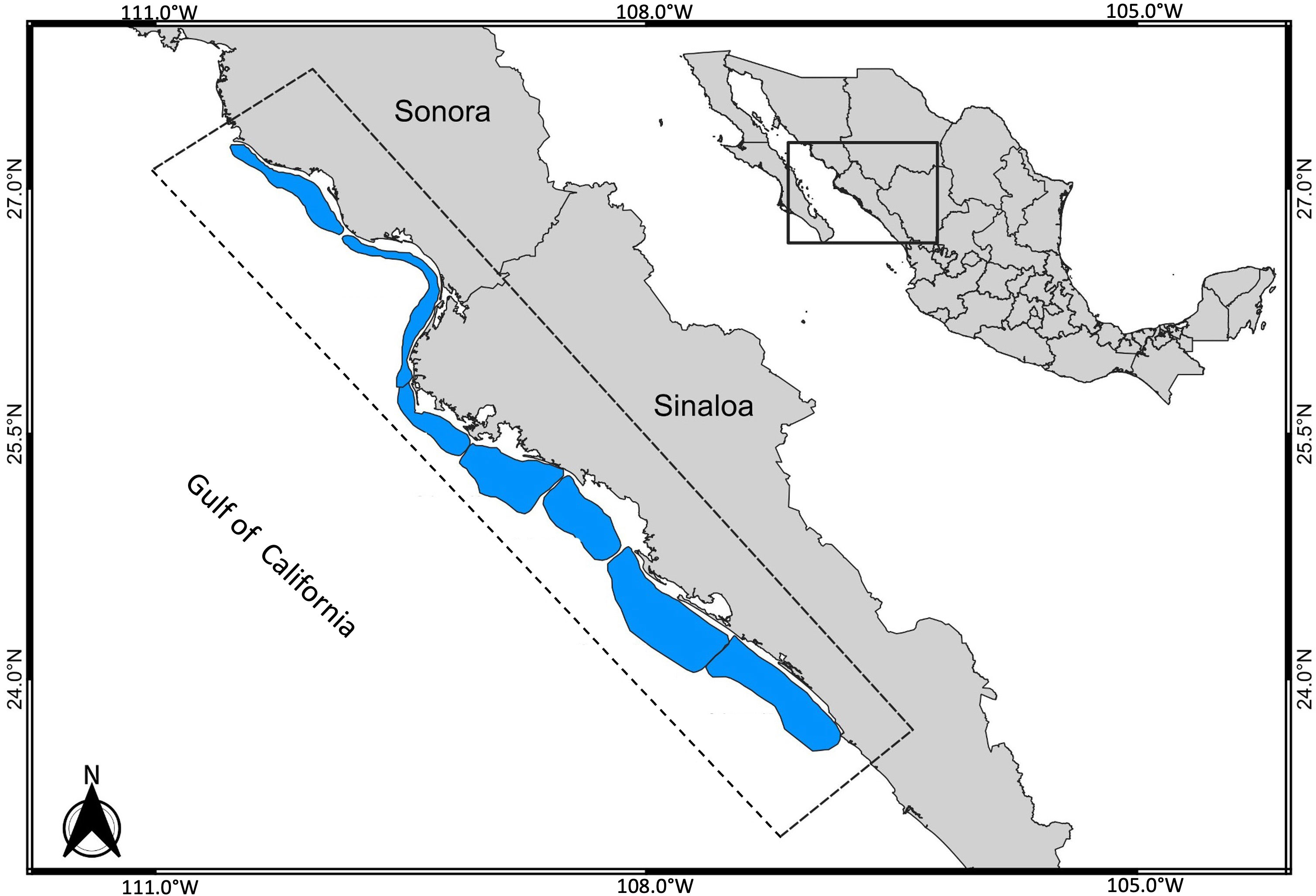
Figure 1 Study area in the central-eastern region of the Gulf of California where the blue shrimp, (Penaeus stylirostris), fishery is located; two fleets participate (one small-scale fleet and one industrial fleet, based on trawling boats).

The fishing season begins in September and ends in March (DOF, 2018), and the main objective of the closed season is to protect the breeding population. Since it is a population with annual longevity, it is assumed that the abundance of the population at the end of the fishing season corresponds to the spawning stock on which the recruitment success depends. In the absence of more information, the best approximation of the recruitment is the size of the stock, which can be approximated from the catch per unit effort at the beginning of the fishing season.

Blue shrimp require shallow and estuarine habitats as nursery grounds, and marine waters for maturity and reproduction. Interannual changes in abundance are affected by environmental patterns such as the Pacific Decadal Oscillation, sea surface temperature, rainfall, upwelling (Aragón-Noriega, 2007; Castro-Ortiz and Lluch-Belda, 2008; Almendarez-Hernández et al., 2015); as well as by regional circulation patterns that affect larval distribution and recruitment (Calderón-Aguilera et al., 2003), which confirms that the carrying capacity is variable between years.

2.2 Method of analysis, the theoretical approach

The data includes records of the two fleets operating every month during the fishing seasons. More than 80% of the blue shrimp yields were taken at depths less than 20 m (54% between 10 and 13 m; and 97% up to 30 m) (Muñoz-Rubí et al., 2023). For this reason, and in the absence of other data, the operation scheme assumed for the analysis is that the two fleets use the same resource in time and space. Given this assumption and that the fleets operate with different fishing boats and gears, it is assumed that if the fleets had the same fishing power, the catch per unit effort per month should be $U_{i,m}=b·U_{j,m}$, where $U$ is the catch per effective day of fishing, $i$ and $j$ represent the two fleets, and $m$ is the monthly time unit during the fishing seasons. If the previous assumption were fulfilled, $b$, the slope of the relationship between $U_{i,m}$ and $U_{j,m}$ should be $1$, while if $b\ne 1$, the resulting value of $b$ will correspond to the conversion factor among fleets. In this way, the $U$ data is standardized between fleets.

The Leslie model (Leslie and Davis, 1939; Hilborn and Walters, 1992) is a very useful tool for estimating the catchability per year for a closed population, a criterion that can be assumed in our case study of a species with annual longevity, and an estimate of the size of the population at a time just before starting the stock assessment experiment. For fleet $i$, the model is described by the relation:

$\begin{array}{ll}{U}_{i,t}=q_i{N}_{0,t}-q_i{K}_{t-1}& \text{Equation (3)}\end{array}$

where $U_{i,t}$ is the catch per unit effort at time $t$, in our case a month; $N_{0,t}$ is the size of the population just before the start of the estimation at time $t$; $K_{t-1}$ is the cumulative catch at time $t-1$; and $q_i$ is the catchability coefficient, which is assumed to be constant.

In this way, for a given fleet $i$, the catchability estimator is, for each year, $q_{i, y(m)}$, where $y(m)$ represents the month $m$ at each fishing season (year) $y$, with a similar solution for the larger fleet $j$. On the other hand, the ordinate to the origin in Equation 3, $U_0$, would approximate $N_0$ since $N_0=U_0/q$; similarly, the size of the population each month can be estimated as $N_m=U_m/q$, and the size of the population during the entire fishing season is

$\begin{array}{ll}{N}_y={\displaystyle \sum _{m(sep), y-1}^{m(mar), y}{N}_m}& \text{Equation (4)}\end{array}$

The state of exploitation of the population can be derived from the harvest rate, represented as $HR=C/B$. Theoretically, for a stable population, in a stable environment, MSY is obtained when $HR=0.5$ (Gulland, 1983). For a population with annual longevity, this means that the remaining population can replace losses due to fishing on an annual basis. Based on this concept, an estimator of the state of exploitation of each fishing season can be obtained from the relationship $C_y/B_y =H{R}_y$ and a similar calculation could be made for each month if it were necessary to know these data.

From this information, a Kobe diagram can be obtained using as a reference point an estimator of the limit rate of population renewal, $PR{R}_{Lim}$ and the state of exploitation given by the estimated harvest rate. The $PR{R}_{Lim,y}$ is obtained from the relationship between the recruitment rate, ${\rho }_y$, at the beginning of the fishing season with respect to the survival ratio of the cohort, $s_y,$ represented by the ratio between the abundance in the last month of the fishing season with respect to the accumulated biomass at the end of the fishing season, $B_y$. The base assumption in this relationship is when $s_y={\rho }_y$; that is, the stock level is analogous to that defined as the replacement level, or the level of recruitment necessary to maintain a population with constant density (Shepherd, 1982; Daan, 1988; Mace and Sissenwine, 1993; Garcia, 1996). With the information available from our case study, $s_y$ and ${\rho }_y$ can be estimated as follows:

$\begin{array}{ll}{s}_y=Ln\left[\left(\frac{B_{mar,y}}{B_y}\right)+1\right]& \text{Equation (5)}\end{array}$

$\begin{array}{ll}{\rho }_y=Ln\left[\left(\frac{B_{mar,y}}{B_{oct,y+1}}\right)+1\right]& \text{Equation (6)}\end{array}$

and

$\begin{array}{ll}PR{R}_{Lim,y}=\raisebox{1ex}{${\rho }_{Lim,y}$}\!\left/ \!\raisebox{-1ex}{$s_{Lim,y}$}\right.=Ln\left(\frac{B_{oct,y+1}}{B_y}\right)& \text{Equation (7)}\end{array}$

where $B_{mar,y}$ represents the biomass in the last month of the fishing season (March) corresponding to breeding adults, while $B_{oct,y+1}$ represents the biomass in the month just before the start of the fishing season corresponding to recruits.

Then, $PR{R}_{Lim,y}=\raisebox{1ex}{${\rho }_{Lim,y}$}\!\left/ \!\raisebox{-1ex}{$s_{Lim,y}$}\right.=1$, and the Kobe diagram can be constructed with $H{R}_y$ in reference to $s_y$ or to ${\rho }_y$ levels when $s_y={\rho }_y$, conditions represented by $s_{Lim,y}$ and ${\rho }_{Lim,y}$

2.3 Considerations of environmental effects

One of the characteristics of short-lived populations is their dependence on the environment. In the case of penaeid shrimp, this feature has been widely reported in the literature (Garcia, 1988; Garcia, 1996; Arreguin-Sanchez et al., 2015; Diop et al., 2015; Lopes et al., 2018), including climate variability and its effects on blue shrimp populations the Gulf of California (Galindo-Bect et al., 2000; Castro-Ortiz and Lluch-Belda, 2008; Perez-Arvizu et al., 2009; Santamaria-del-Angel et al., 2011; Páez-Osuna et al., 2016; Cota-Durán et al., 2021). In the case study, given the evidence reported in the literature, a brief analysis of the contribution of environmental variability in the context of the Kobe diagram, particularly related to $PR{R}_{Lim}$, is provided. In the present case study, two environmental variables associated with specific biological processes were considered: primary production represented by the concentration of chlorophyll-a, $Chl\_a$, which is associated with survival throughout the fishing season, as an index of food availability, and sea surface temperature March ($SS{T}_{mar}$), which is associated with reproductive success and, consequently, with recruitment success.

2.4 Assumptions and considerations for assessment methods

Since only monthly catch and effort data are available each year and blue shrimp is a species with annual longevity, it is necessary to make some assumptions about stock assessment. A sequentiality in the operation of the fleets is generally assumed, meaning the small-scale fleet retains smaller organisms than the industrial fleet. In this context, it is also assumed that the operation of the small-scale fleet starts before the industrial fleet, depending on the migration process of the species and its growth. In the case of the blue shrimp, as seen in the available data supply (capture in weight but without size structure and effective fishing days as fishing effort), the fishery does not exhibit this operational scheme (as can be seen in S1). Fishing in coastal waters up to 5 fathoms (9.15 m) deep is prohibited; and from that depth, both fleets begin to operate. In the case study, the data do not show a time lag among fleets and sequentiality is not considered (see Supplementary materials S1).

Reproduction occurs between June and August (Aragón-Noriega and García-Juárez, 2002; Calderon-Aguilera et al., 2003; Lopez-Martinez et al., 2005; Aragón-Noriega, 2007); therefore, recruitment to the fishery is reflected at the beginning of the fishing season since there is a single annual cohort. According to the available data (catch and effort data), in September, when the fishing season begins, the small-scale fleet retains 43% of the annual catches, while the industrial fleet retains 39%. On the other hand, the Leslie model (Leslie and Davis, 1939; Hilborn and Walters, 1992) was initially developed for individual counts. In our case study, the model is solved with biomass data so that Equations 3 and 4 are defined as follows:

$\begin{array}{ll}{U}_{i,t}=q_i^{\prime }{B}_{0,t}-q_i^{\prime }{k}_{t-1}& \text{equation (3')}\end{array}$

and

$\begin{array}{ll}{B}_y={\displaystyle \sum _{m(sep), y-1}^{m(mar), y}{B}_m}& \text{equation (4')}\end{array}$

where $q^{\prime }\ne q$ given the units in each case, one referring to the number of individuals and the other to biomass units, and $k$ represents the cumulative capture in weight. Parameters $q_t^{\text{'}}$ and $B_{0,t}$ in equation (3’) can be estimated by regression or some analogous procedure.

This method assumes that the assessment experiment is carried out on a closed population, where recruitment occurs only at the beginning of the season and no later, and there is no migration to the area during the time of the experiment. In the case study, this assumption is acceptable since it is an annually closed population. Additionally, an assumption that is not generally made explicit is natural mortality, in the case of the model, it is assumed to be constant so that the trend for the “depletion rate” represents changes in fishing mortality rate.

The model assumes a constant average annual catchability rate, although conceptually, several sources of catchability variation have been mentioned in the literature (Arreguín-Sánchez, 1996; Arreguín-Sánchez and Pitcher, 1999). Consider in equation 3’, for a year $y$, that $U_y=q_y{E}_y$, where $U_y$ represents the relative abundance of the stock in biomass, and $E_y$ the fishing effort. Then, $q_y$ is a coefficient representing the interaction between the stock and the fishing effort, such that anything that affects $U_y$ and $E_y$ also affects $q_y$.

There is not a single level of replacement given the variability of the stocks (Shepherd, 1982), especially in exploited stocks showing interannual variation; in these cases, there is a different level of replacement according to each annual recruit/adult combination. This concept is especially valid for species with annual longevity and is especially critical for $PR{R}_{Lim,y}$ estimation. In this sense, the conventional assumption of a stable carrying capacity is not appropriate for these estimates, and the annual value of $PR{R}_{Lim,y}$may be estimated each fishing season.

3 Results

3.1 Observed data

Figure 2 shows the monthly trends of the observed data for catch ($C_{m,y}$), effort ($E_{m,y}$) and catch per unit effort $U_{m,y}$ for each fishing season and fleet, while data are provided as Supplementary material S1, and the global patterns for all fishing seasons are shown in Supplementary materials S2, Supplementary figure S2.1.

FIGURE 2

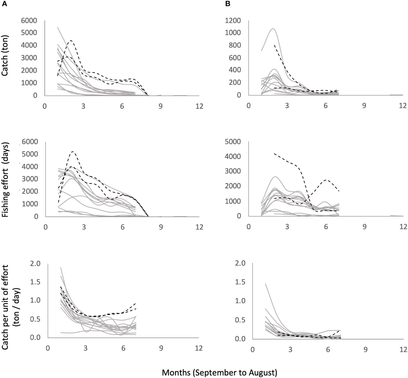
Figure 2 Observed data catch (${\text{C}}_{\text{m},\text{y}}$), effort (${\text{E}}_{\text{m},\text{y}}$) and catch per unit effort ${\text{U}}_{\text{m},\text{y}}$ for the small-scale fleet (A) and industrial fleet (B) during the fishing seasons from 2006/2007 to 2018/2019 (gray lines). The dotted black lines show the COVID-19 pandemic years (2019-2020 and 2020-2021). Note the anomalous behavior in ${\text{E}}_{\text{m},\text{y}}$ for these last fishing seasons.

As previously mentioned, two fleets participate in the fishery, one small-scale, $ssf$, and the other industrial, $ind$; and it is assumed they compete for the same resource. In both cases, the effort is recorded as an effective day of fishing; however, given the difference in equipment, boats and fishing gear, a conversion was made to standardize the fishing effort across fleets. An example of such standardization is given in S2, Supplementary figure S2.2.

Assuming the fleets operate simultaneously in time and space and that the $U$ is a measure of relative abundance, then the fishing effort of a fleet could be estimated from the following equality.

$\begin{array}{ll}\frac{C_{ind,m,y}}{E_{ind,m,y}}=\frac{C_{ssf,m,y}}{E_{ssf,m,y}}& \text{Equation (8)}\end{array}$

Since this equality is not fulfilled (because of the differences in fishing power and gear used by the fleets), the effort of the small-scale fleet can be estimated in the units of the industrial fleet as follows:

$\begin{array}{ll}{E}_{ssf\_st,m,y}=\frac{C_{ssf,m,y}}{C_{ind,m,y}}·E_{ind,m,y}& \text{Equation (9)}\end{array}$

In this way, the $U_{ssf\_st,m,y}$ the standardized ($\text{st}$) $\text{U}$ in terms of the units of effort of the industrial fleet.

3.2 Catchability, stock size and harvest rate

Once the information was standardized, the catchability was estimated for each fleet and year. For this, the Leslie and DeLury model (Leslie and Davis, 1939; Hilborn and Walters, 1992) was used showing some examples in Supplementary figure S2.3 within S2. Figure 3 shows the values of catchability by fleet and year. The order of magnitude for the first three fishing seasons considered (2005/6, 2006/7 and 2007/8) was clearly higher than that for the other seasons. However, when considering the 2010/11 fishing season, an apparent decreasing pattern is observed, which is more accentuated for the industrial fleet.

FIGURE 3

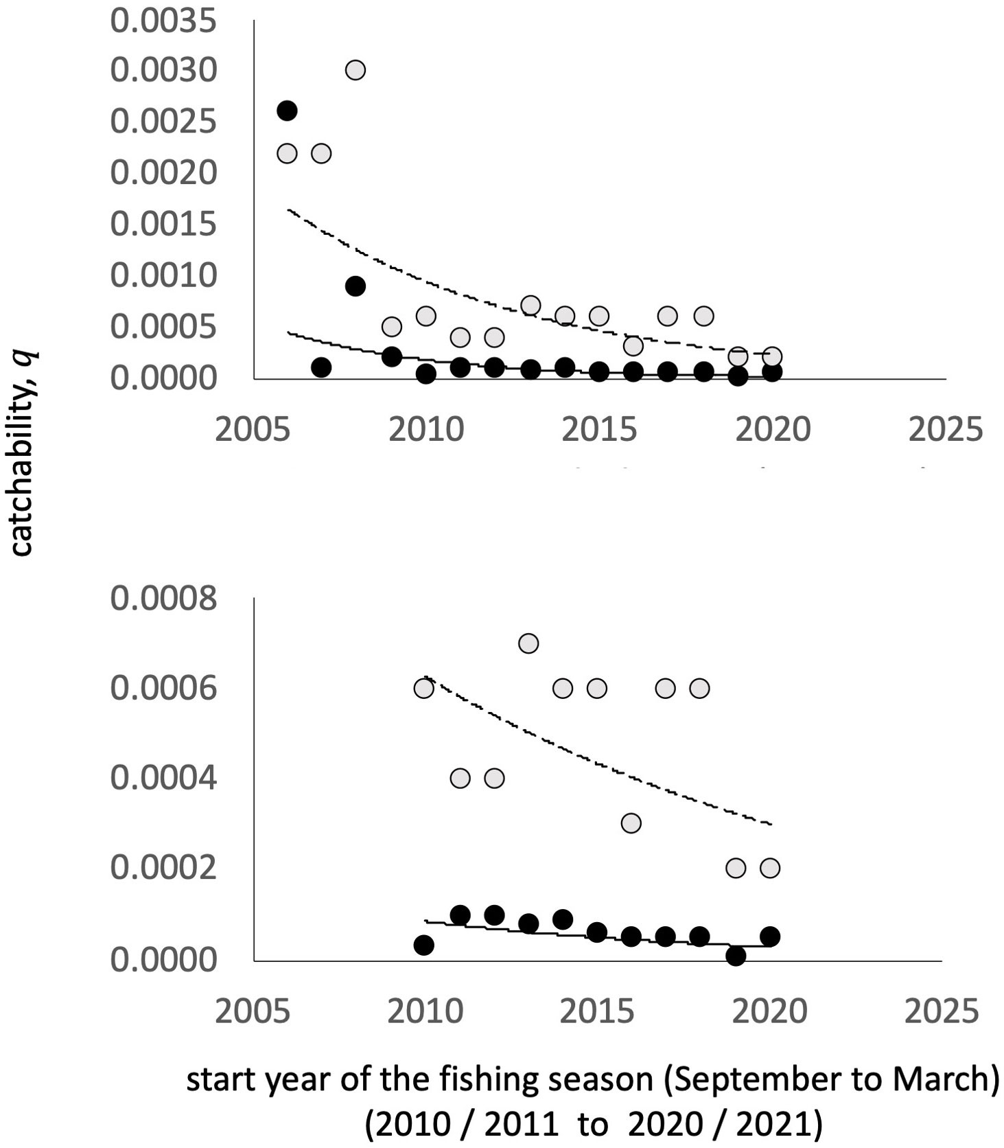
Figure 3 Estimates of catchability by fishing season and fleet for the blue shrimp fishery in the central-eastern Gulf of California. An apparent decreasing pattern is observed over time for both fleets (below), which is accentuated in the industrial fleet. The gray dots represent the catchability estimates for the industrial fleet and the black dots for the small-scale fleet.

The capture is defined as $C=qEB$ (Gulland, 1983), such that $B=\raisebox{1ex}{$C$}\!\left/ \!\raisebox{-1ex}{$qE$}\right.=\raisebox{1ex}{$U$}\!\left/ \!\raisebox{-1ex}{$q$}\right.$. This relationship is used to estimate the biomass, monthly, by fleet, or for the total fishery (adding the estimated biomass individually for each fleet), and for all fishing seasons. In this way, estimates of the decline of the biomass of the shrimp population from the beginning to the end of the fishing season and for the accumulated biomass during the entire fishing season are obtained (Figure 4). The estimates of $q_y$ and $B_y$ are shown in Supplementary material S3.

FIGURE 4

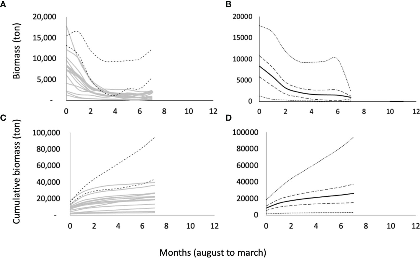
Figure 4 Biomass estimates for each blue shrimp fishing season in the central-eastern Gulf of California. (A, B) biomass decay by fishing season and general pattern of biomass change throughout the fishing season, respectively. (C, D) Cumulated biomass per fishing season and general pattern, respectively. (A, C), dashed lines represent the COVID-19 pandemic fishing seasons. (B, D) inner dashed lines represents 95% confidence intervals and external minimum and maximum values.

Given the values of $C_{m,f,y}$ and $B_{m,f,y}$, an estimate of the corresponding harvest rate for each month was obtained, $H{R}_{m,f,y}$, and from its average, an estimate for the year, $H{R}_y$. On the other hand, from the annual catch $C_y$ and biomass $B_y$, a second annual harvest rate estimate was obtained, $H{R}_y^{\text{'}}$. Figure 5 shows the trends of the values of the two harvest rates for fishing seasons.

FIGURE 5

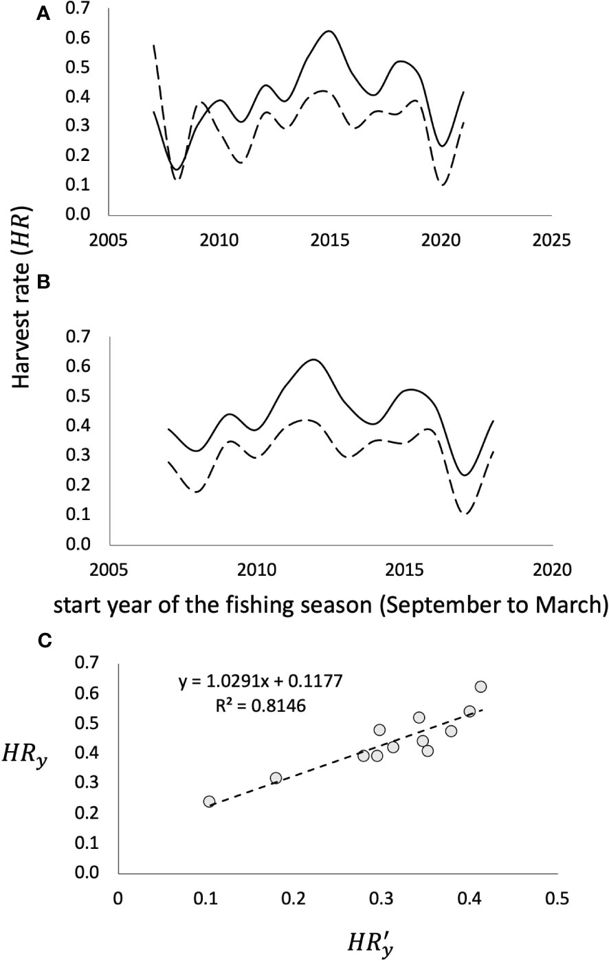
Figure 5 Harvest rate estimates by fishing season during the entire time period studied (A) and from the 2010-2011 and 2020-2021 fishing seasons (B). The continuous line corresponds to the estimate of HR_y (monthly average), while the dashed line corresponds to the estimates of HR_'y (annual). (C) relationship between annual harvest rates; derived from the average of monthly Catch/Biomass ratios (HRy), and the annual Catch/Biomass (HRy′), showing that there is no statistically significant difference (p<0.05) between them.

The estimation form for $H{R}_y$ and $H{R}_y^{\text{'}}$ resulted in slightly different values for each fishing season (Table 1). The same Figure 5 shows the relationship between both estimates, resulting, on average, in $H{R}_y>H{R}_y^{\text{'}}$, which, according to the relationship shown in Figure 5, $H{R}_y\approx 1.029·H{R}_y^{\text{'}}$.

TABLE 1

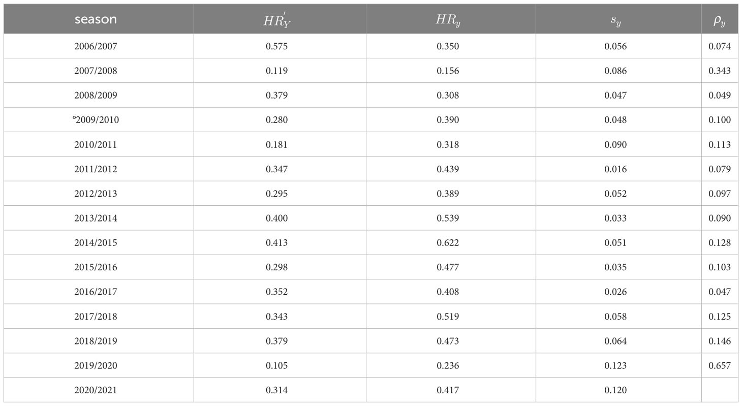
Table 1 $H{R}_y^{\text{'}},$Harvest Rates estimated from the average monthly catch and biomass; $H{R}_y$ estimated from annual data; ${\text{s}}_{\text{y}}$ survival ratio, and ${\rho }_y$, recruitment rate,; all by fishing season.

3.3 Estimates of survival rates, S_y, and recruitment, P_y

Two quantities of interest for management can be estimated from the monthly biomass data for each fishing season; one of them refers to the recruitment to the fishery, which occurs in September, at the beginning of the fishing season, and represents the reproduction success and the other is the survival of the cohort, which represents the remaining biomass at the end of the fishing season. The proportion of the stock surviving at the last month of the fishing season is an indicator of the remaining biomass of adults whose reproductive success will lead to recruitment to the following fishing season.

Equations 5 and 6 represent estimators of the survival ratio and recruitment rate, respectively, obtained from the estimated monthly biomasses. Figure 6 shows the recruitment rate and survival ratio, both as a function of the remaining biomass at the end of each fishing season $B_{mar,y}$ (S3). For the estimations we assume biomass $B$ can be approached by catch per unit of effort data $U$, for the needed times.

FIGURE 6

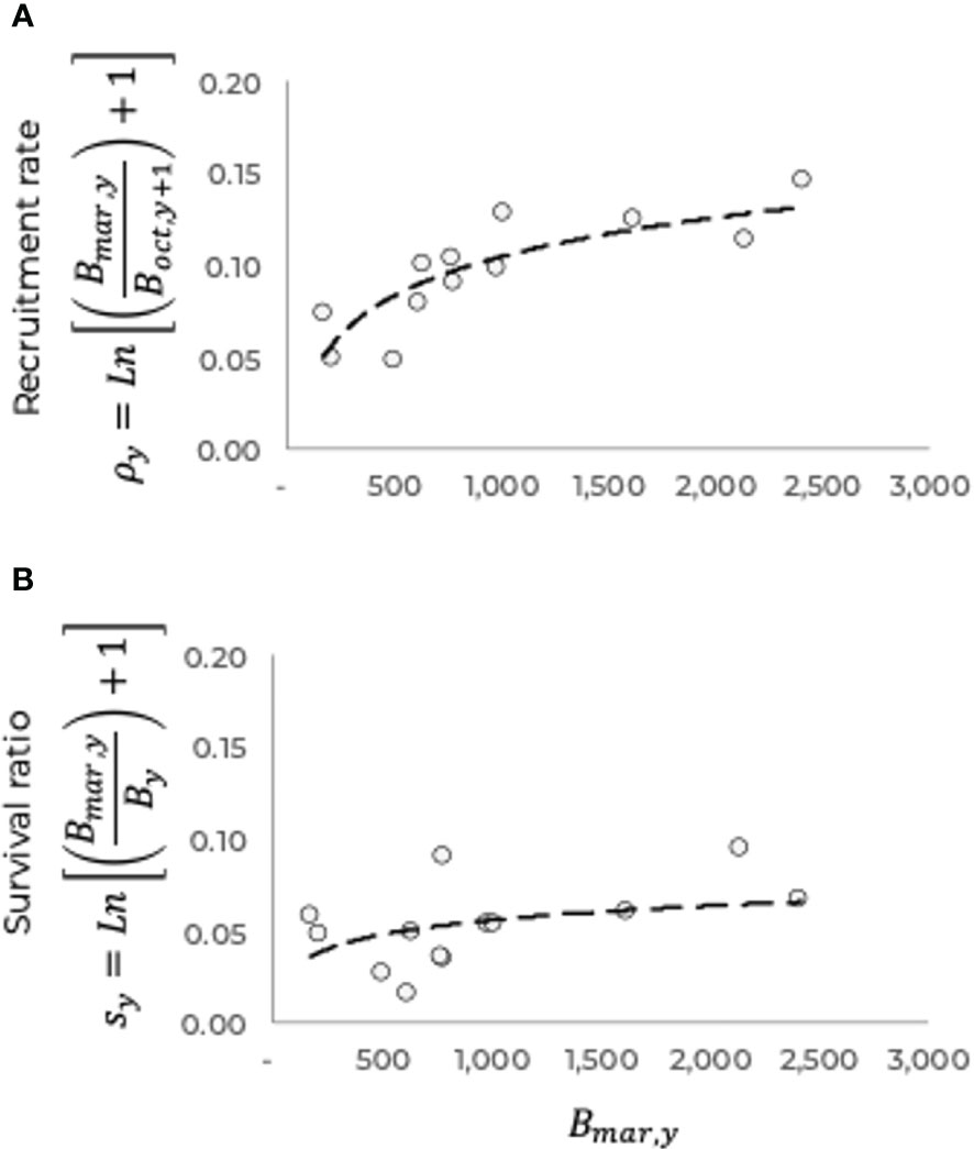
Figure 6 Recruitment rate (A) and survival ratio (B) as a function of the remaining biomass, ${\text{B}}_{\text{mar},\text{y}}$ (reproducers) at the end of the fishing season of the blue shrimp population of the central-eastern region of the Gulf of California.

3.4 Estimation of the limit reference point, PRR_Lim,y (replacement)

The relationship between the recruitment rate, ${\rho }_y$, and the remaining spawning biomass, $B_{mar,y}$, toward the end of the fishing season suggests a stock-recruitment relationship where density-independent processes predominate Beverton and Holt (1957). The same type of relationship appears with respect to survival ratio ${\text{s}}_{\text{y}}$, showing some stability around ${\text{s}}_{\text{y}}=0.062$(crossing point in Figure 7). According to Figure 6, and regarding the α value referred to survival ratio in Figure 5, the remaining biomasses greater than 1,500 tons would not have a significant impact on survival, while remaining biomass, less than 1,000 tons, could affect the survival rate. Figure 7 shows the relationship between ${\rho }_y$ and ${\text{s}}_{\text{y}}$, where the bisector of these relationships reflects, analogously, the replacement level (Mace and Sissenwine, 1993; Garcia, 1996) in such a way that the crossing point between the trend of the observed relationship with the bisector can be interpreted as a limit reference point, in this case defined as the limit rate of renewal of the population, $PR{R}_{Lim}$, which represents the replacement level. It is assumed that the ${\text{s}}_{\text{y}}$ corresponding to $PR{R}_{Lim}$ is the size of the remaining spawning biomass necessary to produce the recruitment level that will eventually replace the stock and the spawning biomass necessary for the persistence of the population. The estimate for $PR{R}_{Lim}$ in Figure 7, in terms of the survival rate, was $s_y=0.073$, while the maximum given by the upper confidence interval (95%) is $PR{R}_{Lim,max}$, $s_y$= 0.106. Note that point $\beta$ in the figure representing $PR{R}_{Lim,max}$ could be identified, if necessary, as a limit based on a precautionary approach.

FIGURE 7

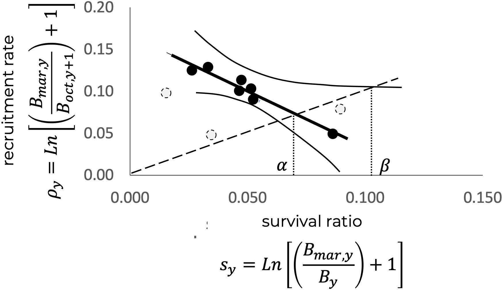
Figure 7 Relationship between the recruitment rate, ${\text{ρ}}_{\text{y}}$, and the survival ratio, ${\text{s}}_{\text{y}}$. The crossing with the bisector, indicated by $\text{α}$, represents the limit reference rate, ${\text{PRR}}_{\text{Lim}}$, corresponding to the replacement level of the population, while β represents ${\text{PRR}}_{\text{Lim},\text{max}}$, as a precautionary criterion. The points in gray were not included in the estimation.

3.5 Kobe diagram

As previously mentioned, the estimations of $s_y$ and ${\rho }_y$, as well as the estimated annual harvest rates, $H{R}_y$, allow the construction of a Kobe diagram, as shown in Figure 8, where the reference levels correspond to $PR{R}_{Lim}$; in this case, relative to the survival ratio, where $s_y=0.073$. and for $s_{y,max}=0.106$. Additionally, Figure 9 shows the Kobe diagrams corresponding to $PR{R}_{Lim}$ relative to the recruitment rate, with ${\rho }_y=0.073$. and ${\rho }_y=0.106$.

FIGURE 8

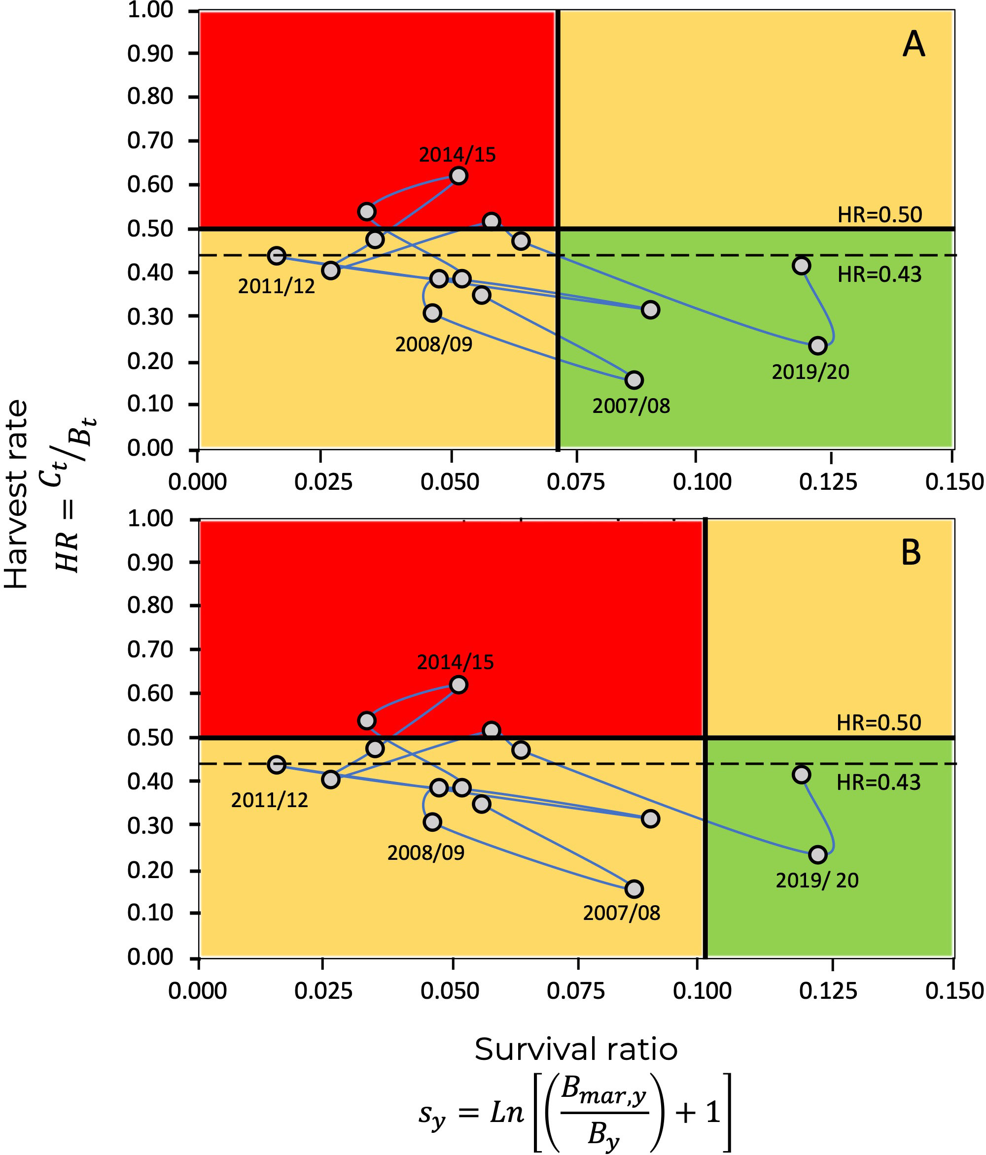
Figure 8 Kobe plot for the blue shrimp fishery in the central-eastern Gulf of California, showing the evolution of the fishery through harvest, ${\text{HR}}_{\text{y}}$ and survival ratio ${\text{s}}_{\text{y}}$. The limit reference point, ${\text{PRR}}_{\text{Lim}}$, is given by the values ${\text{s}}_{\text{y}}=0.073$ (A) and ${\text{s}}_{\text{y},\text{max}}=0.106$ (B). The continuous horizontal line represents the limit harvest rate of $\text{HR}=0.50$, while the dashed Line a $\text{HR}=0.43$ corresponds to the limit harvest rate defined from ecosystem attributes (organization and function) (Arreguín-Sánchez, 2022a).

FIGURE 9

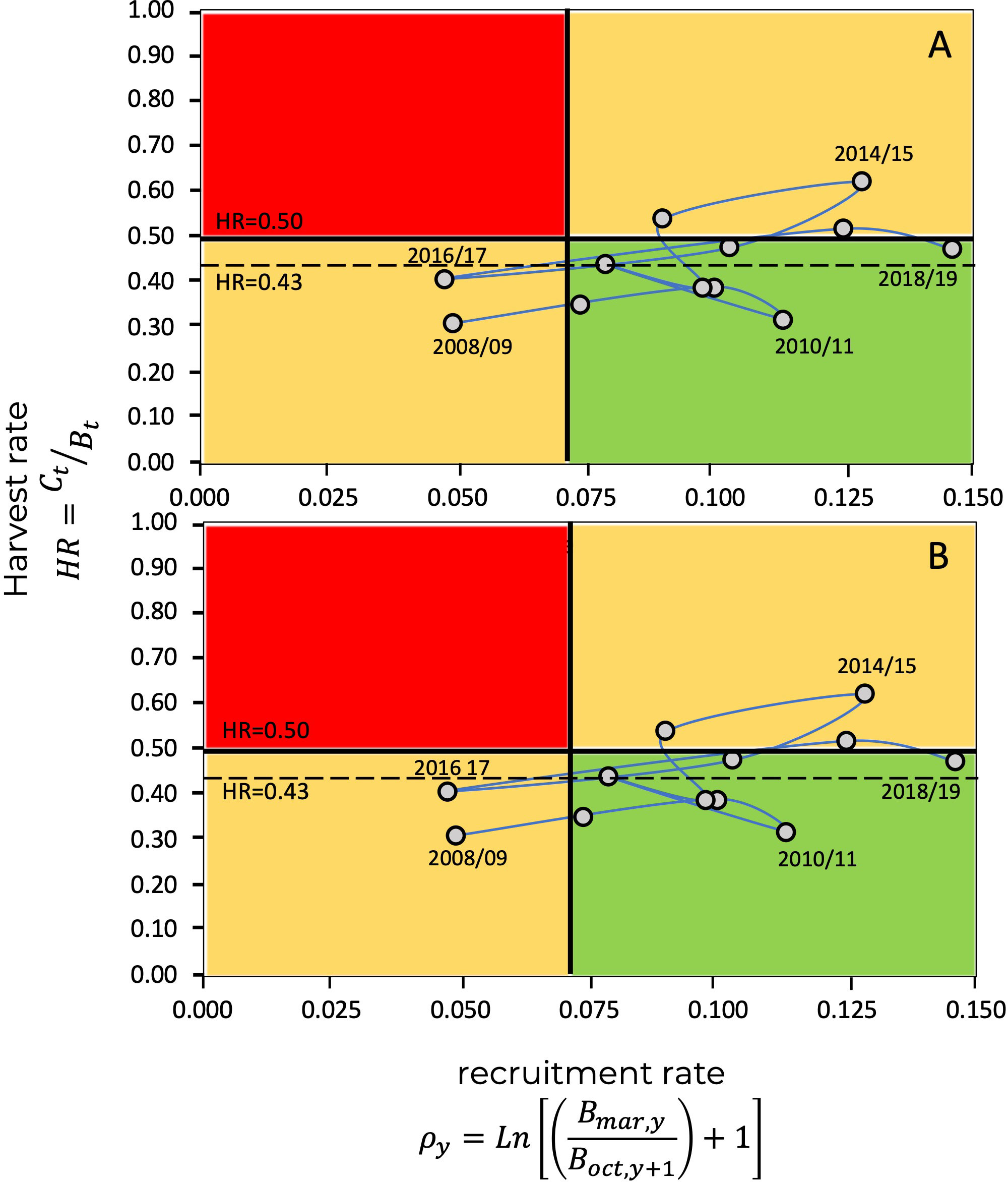
Figure 9 Kobe plot for the blue shrimp fishery in the central-eastern Gulf of California, showing the evolution of the fishery through harvest rates, ${\text{HR}}_{\text{y}}$ and recruitment rate, ${\text{ρ}}_{\text{y}}$. The limit reference point, ${\text{PRR}}_{\text{Lim}}$, is given by the values ${\text{ρ}}_{\text{y}}=0.073$ (A), and ${\text{ρ}}_{\text{y}}=0.106$ (B), as a precautionary criterion. The continuous horizontal line represents the limit harvest rate of $\text{HR}=0.50$, while the dashed line represents $\text{HR}=0.43$, defined from ecosystem attributes (ecosystem organization and functioning) (Arreguín-Sánchez, 2022a).

In the Kobe diagrams, the harvest rate, $HR$, is used as an indicator of the state of exploitation of the population, representing the ratio among catch and the available biomass. In this context, the values of $HR>0.5$ assume overfishing since the remaining population will not be able to replace the losses due to fishing. Additionally, a limit harvest rate value derived for shrimp from ecosystem attributes (organization and function) is taken as an precautionary criterion, in this case $HR=0.43$ (Arreguín-Sánchez, 2022a).

3.6 Environmental variability contribution

Statistically significant polynomial relationships were found between survival ratio, $s_y$, and $Chl\_a$; and between recruitment rate, ${\rho }_y$, and $SS{T}_{mar}$ (see figures in S2 and data of the anomalies of $Chl\_a$ and $SS{T}_{mar}$ in S3). These relationships were used to estimate theoretical values for $s_y$ and ${\rho }_y$ and estimate a new $PR{R}_{Lim}$ influenced by the environment (Figure 10).

FIGURE 10

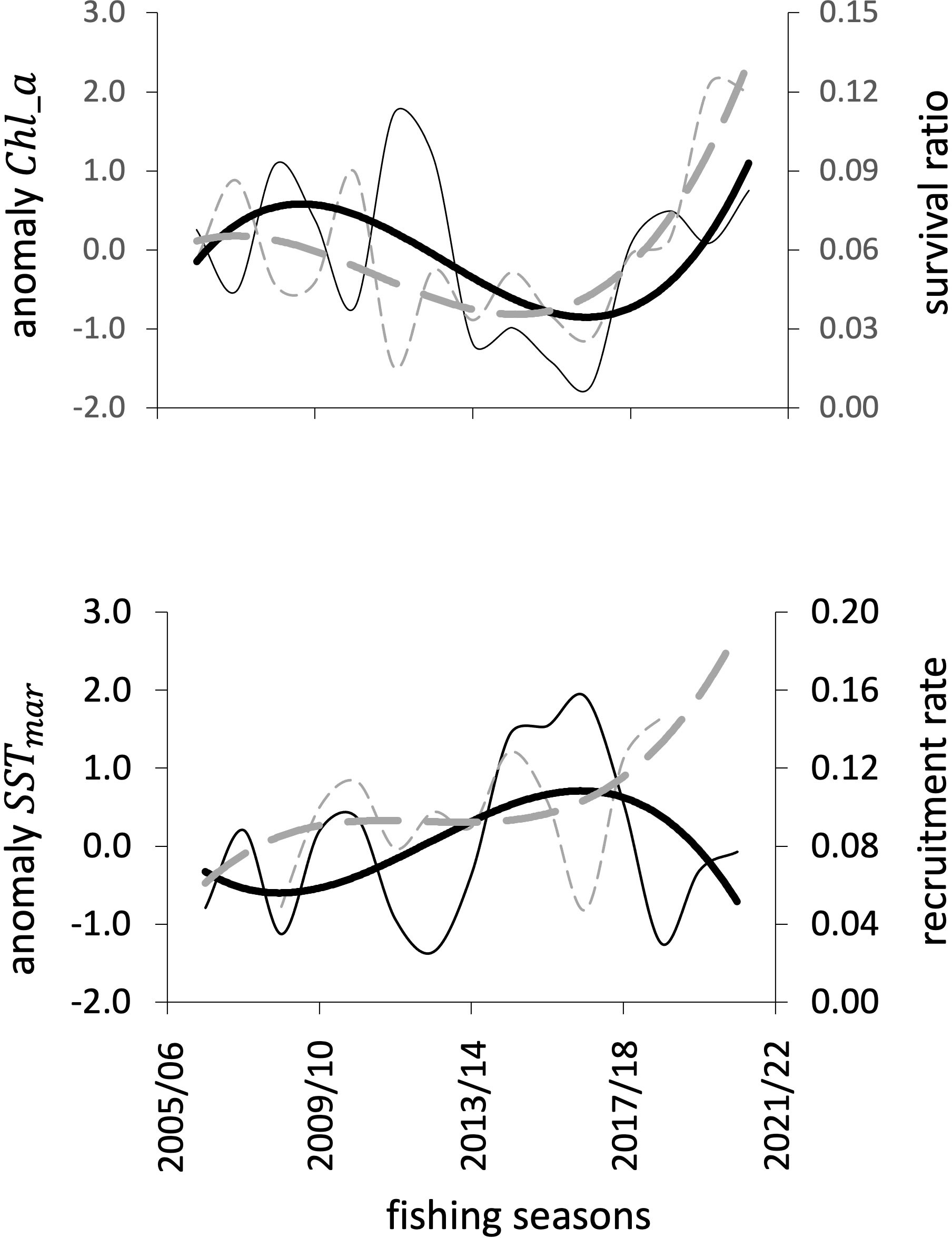
Figure 10 Above, the interannual pattern of ${\text{s}}_{\text{y}}$ and its relationship with the anomaly of $\text{Chl}\_\text{a}$. Below, the interannual pattern of ρ_y and its relationship with the anomaly of ${\text{SST}}_{\text{mar}}$. Black lines represent the environmental variable, while the gray lines show indices related to population changes. Thin lines are the observed data; thick lines show smoothing. Note, the patterns in the thick lines; above, almost parallel trends, while below, opposite trends.

From the information of the anomalies of $Chl\_a$ and $SS{T}_{Mar}$, their rate of change was obtained, which was used to adjust the relative values of $s_y$ and ${\rho }_y$ (see figure illustrating the difference with and without the environmental contribution in S2, Supplementary figure S2.4).

With the above information and to estimate the partial contributions of the environment in the estimation of the limit reference point, the relationship between ${\rho }_y$ and $s_y$ was reconstructed in the absence of an environmental effect to estimate an alternative $PR{R}_{Lim}^{\text{'}}$. The result is shown in Figure 11, where for $PR{R}_{Lim}^{\text{'}}$, the value of $s_y^{\text{'}}=0.068$was estimated. Accordingly, the difference between $PR{R}_{Lim}$ and $PR{R}_{Lim}^{\text{'}}$ (with and without environmental effects) is approximately 7%, where $PR{R}_{Lim}>PR{R}_{Lim}^{\text{'}}$.

FIGURE 11

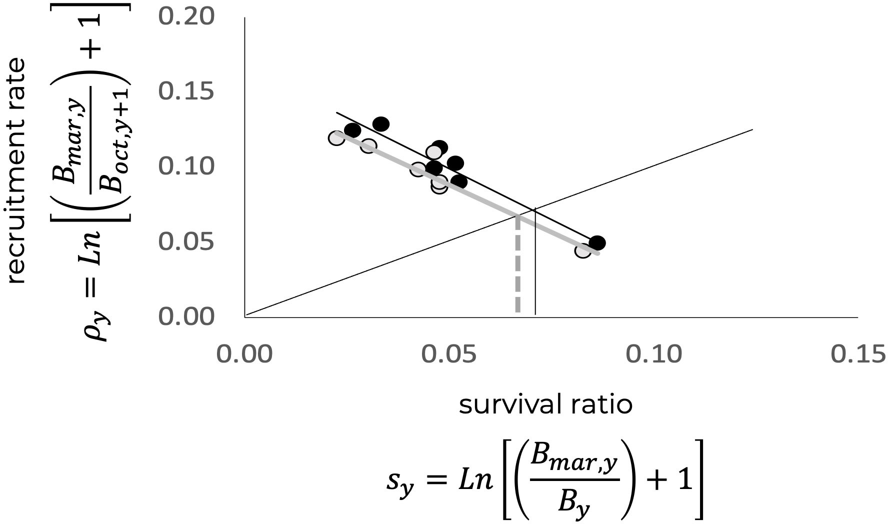
Figure 11 Relation between the recruitment rate and the survival rate. The crossing with the bisector represents the limit reference rate, $PR{R}_{Lim}$, which corresponds to the replacement level of the population. Black and gray lines represent without and with environmental effects, respectively. Crossing points in terms of the survival ratio are shown, where s_y and $s{\text{'}}_y$ represent conditions with and without environmental effects, respectively, with $s_y$> $s{\text{'}}_y$.

3.7 Kobe diagram and environmental contribution

The position relative to the state of exploitation of the blue shrimp resource throughout the evolution of the fishery in the Kobe diagram changes slightly when considering the effects of the environment. Figure 12 shows the Kobe diagram as a function of $s_y$ and ${\rho }_y$, showing the relative position of the $PR{R}_{Lim}$ in respect the replacement level and the corresponding harvesting rates. In addition, Figure 12 shows the $PR{R}_{Lim}$ by considering the population and ecosystem perspectives. Such $PR{R}_{Lim}$ contrasts can be useful for management, particularly by considering precautionary approach into the decision-making process.

FIGURE 12

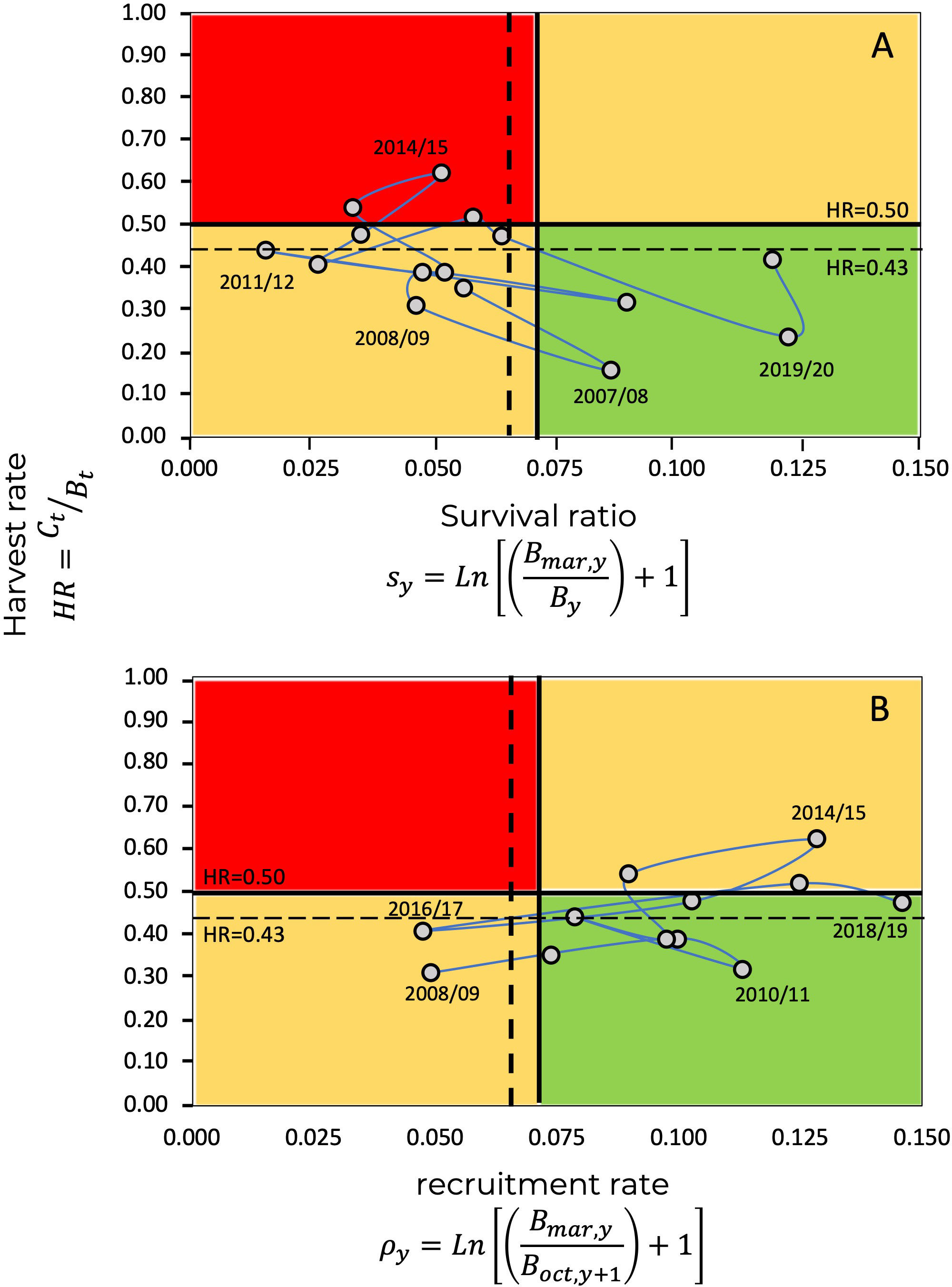
Figure 12 Kobe plot for the blue shrimp fishery in the central-eastern Gulf of California, showing the evolution of the fishery through harvest, $H{R}_y$ and respect survival ratio, $s_y$, and recruitment rate, ${\rho }_y$. The limit reference point, $PR{R}_{Lim}$, with (vertical continuous line) and without (vertical dashed line) environmental effect, and $s_y={\rho }_y=0.073$ (A), and $s_y={\rho }_y=0.068$ (B), respectively. The continuous horizontal line represents the population limit $HR=0.50$.

4 Discussion

4.1 Adapting stock depletion method

In the introduction section, mention was made of the methodological conflict when attempting to use the biomass dynamic models for short-lived species (see equation 2). To address this problem, other approaches have been proposed, such as depletion models, which are based on the Leslie and Davis (1939) model following the solution proposed by Chapman (1974) given by the relationship,

$\begin{array}{ll}{C}_t=q{E}_t\left(N_0{e}^{-M_t}-e^{-\frac{M}{2}}\left(\sum _{i=1}^{i=t-1}{C}_i{e}^{-M(t-i-1)}\right)\right)e^{-\frac{M}{2}}& \text{Equation (10)}\end{array}$

which, as proposed by Pope (1972), assumes that capture occurs in the middle of the time periods being $t$ a given time interval, $i$ refers to the number of time intervals, $M$ is the natural mortality rate, and the catch, $C$, is expressed in number of individuals.

Depletion methods have been applied to various fished stocks (Rosenberg et al., 1990; Roa-Ureta and Arkhipkin, 2007; Maynou, 2015; Roa-Ureta, 2015; Arkhipkin et al., 2021); where the solution of equation (10) requires a little more information compared to the procedure proposed in this work. For example, to express $C$ in numbers, it is necessary to know the average weight of the individuals, or the size structure of catch, and the weight-length relationship. Likewise, an independent estimate of $M$ is required. With this base, equation 10 is solved for $N_0$ and $q$. In the procedure proposed in this paper, the $q^{\prime }$ and $B_0$ were estimated based on weight (biomass) and were obtained by regression, although any other analogous procedure may be applied if deemed convenient. Additionally, in this work, some population performance indices were proposed, derived from $U_t$ data, such as survival and recruitment rates. These indicators were used to estimate biological reference points and construct Kobe diagrams to identify the state of exploitation of the exploited stocks, and to suggest management trends.

4.2 Available data

Limited data are a challenge for many fisheries for which information on the state of exploitation of fish resources is needed, and typically, one must use the existing information, methods, and analysis tools available. In the case of the blue shrimp fishery in the central-eastern Gulf of California, the information available consists of daily catch records and effective days of fishing for the two fleets, one small-scale and the other industrial, that operate on the continental shelf. Although sequentiality in this fishery is a common assumption, when grouping data monthly by fleet, we found that there was no evidence of sequentiality, since the fishing operations start at the same time, and fit the paradigm of two fleets competing for the same resource. One of the characteristics of sequentiality in shrimp fisheries is that the fleets exploit different life stages, such that the yields of one fleet depend strongly on the fishing intensity of the other through survival; thus, the limits of fishing for one fleet must be defined in such a way that enables the operation of the next fleet. In the available information, there was no evidence of this situation; in contrast, assuming only one recruitment pulse, the fleets seemed to respond simultaneously to it in time and space so that competition between fleets appeared to be a reasonable model.

4.3 Standardization of fishing effort and catchability

If we assume that the fleets operate simultaneously in time and space, the approximation of the standardization of the fishing effort is also reasonable in terms of units of effort (in this case, effective fishing days); however, the fishing power, fishing equipment and gear differ between the fleets, a situation that is reflected in differences in catchability. In the case of the blue shrimp fishery, the probability of retaining a unit of fish resource for a unit of fishing effort is different according to the relative fishing power of each fleet. This is evident when applying the Leslie method (Leslie and Davis, 1939; Hilborn and Walters, 1992); if the fleets had the same fishing power, they would exert the same fishing mortality per effective day of fishing, and the removal of individuals during the capture operations would be similar, followed by catchability. This did not always occur (see Supplementary material S3); the values for the industrial fleet (Figure 3) were always greater, almost 8 times greater for the period from 2010 to 2020.

On the other hand, although variability in catchability has been reported throughout the fishing season and with sizes (Aranceta-Garza et al., 2020), since there is no detailed information available for this study, the constancy assumption is considered acceptable. Note in this context that, beyond the differences in the relative fishing power of each fleet already mentioned above, the cohort effect, which implies variability based on size and season, impacts the two fleets similarly when operating simultaneously in space and time. This last concept is a key assumption for which there is no information available that can be used for estimation.

4.4 Stock size and harvest rate

The estimation of the stock size was initially carried out by fleet, considering the differences in magnitude of the catchability coefficient, and the global estimator of biomass of the stock was obtained by simple addition. This estimate corresponds to the biomass available for fishing and not necessarily to the total biomass of the stock, although, presumably, most of it is accessed by the fleet. Given this condition, for management purposes, the estimated biomass should be considered equal to the stock biomass.

4.5 Estimate of $s_y$, ${\rho }_y$ and limit reference point PRR_Lim,y

Two parameters were of great interest, especially when dealing with a stock with annual longevity. Survival to the last month of the fishing season, represented by $s_y$, indicates the remaining biomass, which, in turn, given the life history, represents the breeding stock whose reproductive success will result in the cohort the following year, which will, in turn, give rise to the stocks for fishing. The other parameter is the recruitment rate ${\rho }_y$, which represents the magnitude of the cohort available for fishing. The interaction between these two concepts establishes a relationship between the remaining biomass of one fishing season and recruitment for the next season (recruitment rate). Thus, the equality $s_y={\rho }_y$ represents the replacement level; that is, the magnitude of recruitment is equivalent to the magnitude of the spawning stock necessary for the population to persist. Consequently, this balance represents the limit reference point for the exploitation of the stock, estimated as $PR{R}_{Lim}=0.073$(crossing point $\alpha$ in Figure 7), meaning the remaining stock at the end of the fishing season must be 7% of that at the beginning of the fishing season. In this sense, exploitation can be developed until reaching that limit level. From Figure 7, and in a precautionary sense, we suggest the limit $PR{R}_{Lim,max}=0.106$(crossing point $\beta$). In terms of survival, this fishing limit was defined as 10% of the remaining biomass at the end of the fishing season. This concept is similar to the strategy defined as proportional escapement (Beddington and Cooke, 1983; Beddington et al., 1990; Rosenberg et al., 1990). Figure 13 illustrates the decline in relative abundance per fleet and total biomass throughout the fishing season. In all cases, the fishery was within the precautionary levels of exploitation.

FIGURE 13

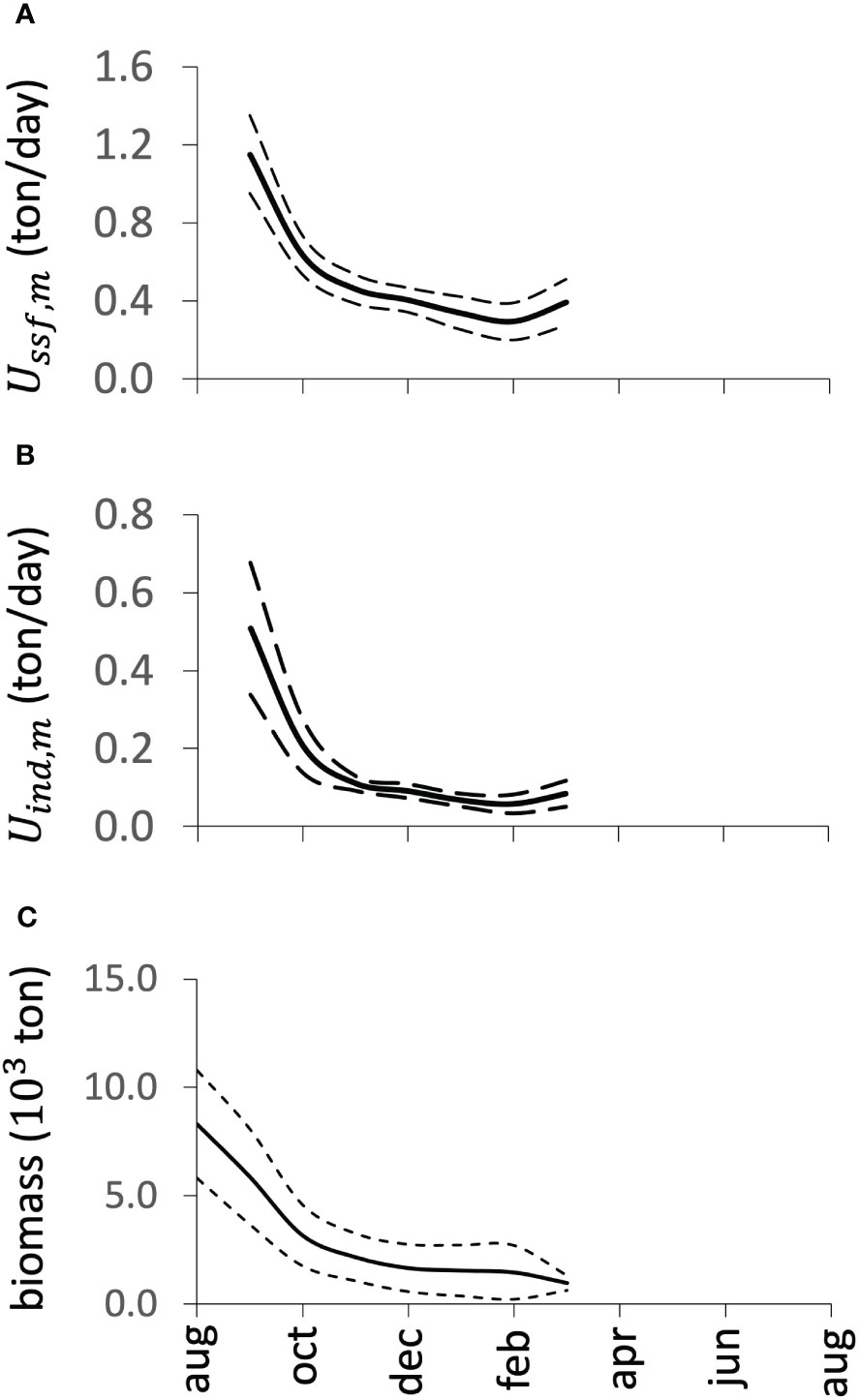
Figure 13 Trends in relative abundance throughout the fishing season, expressed as catch per unit effort, for the small-scale fleet (A) and for the industrial fleet (B). The average of the ratios of the abundances between the end and the beginning of the fishing season is 0.15. Figure (C) represents the decay of the biomass, where the ratio between the biomass at the end and the beginning of the fishing season is 0.12. The dotted lines represent the 95% confidence interval.

The proportions of abundances at the end of the fishing season with respect to the beginning of the fishing season resulted in an escapement of close to 15% of the population, a figure slightly higher than that from the estimated biomass, which was 12%. In contrast, $PR{R}_{Lim}$ suggested values of 7% and 10%, based on a precautionary approach. This means that, in terms of escapement, the fishery is operating at safe levels of exploitation.

4.6 Consideration of environmental effect

The effect of the environment was considered in two ways: through the primary production index expressed annually as $Chl\_a$ concentration and interpreted as an indicator of food availability that could affect survival; and through the surface temperature of March, $SS{T}_{March}$, acting as an indication of the quality of the environment at the time when the reproductive process begins. The anomalies of the two indices were used to identify the contribution of the environment to the variability of the survival and recruitment processes. According to the results, the environment contributed approximately 7% to the estimate $PR{R}_{Lim}$ obtained from the observed data; that is, the one $PR{R}_{Lim}$ without the environmental contribution was defined by lower values of $s_y$ and ${\rho }_y$. As environmental variability, in terms of management, brings uncertainty, the recommendation is to use these estimates of $PR{R}_{Lim}$, within a precautionary management scheme. For the blue shrimp, the $s_y$ and ${\rho }_y$ estimated without environmental effects could also be used to isolate the population response to fishing.

4.7 Kobe diagram

In the Kobe diagrams, when the survival ratio, $s_y$, was used as a criterion, we found that, for the last 15 years, only three exceeded the limit harvest rate of $HR=0.50$, and five exceeded the harvest rate corresponding to the limit reference point based on the ecosystem criteria ($HR=0.43$) (Figure 12). When recruitment rate, ${\rho }_y$, was used as a criterion, no season fell within the critical zone, above $HR=0.50$, and five were located above $HR=0.43$(Figure 12). The interpretation of the Kobe diagram indicates that the state of the blue shrimp fishery in the central-eastern region of the Gulf of California, given in Figure 12, is typical of a sustainable fishery that must be managed by limiting its operation. In the case study, the limit levels for the survival ratio, $s_y$, and the recruitment rate, ${\rho }_y$, fell within the limits of exploitation that permit a sustainable fishery, even under a precautionary approach.

Currently, management measures consider the definition of the closed and start of the fishing season, size of first capture, prohibition of fishing within nursery areas, and controls on fishing gear and methods (DOF, 2018). Although the blue shrimp fishery in the central-eastern region of the Gulf of California is exploited at a level of sustainability close to its maximum production capacity, there is no harvest limit as a reference for management. In terms of the criteria defined in this work, this limit can be established to guarantee sustainability. According to the results, and the recent history of the fishery, it can be established as the limit harvest rate HR=0.43; which implies, in annual terms, that the proportion of capture regarding the biomass of the population must be a maximum of 43%. In practice, this quantity could be established by estimating the initial size of the population at the beginning of the fishing season (September) and monitoring the decline in abundance until reaching a limit of 10% of the initial abundance, which corresponds to the $PR{R}_{Lim}$, estimated in this work considering the survival ratio, recruitment rate and the environmental effects.

Data availability statement

The original contributions presented in the study are included in the article/Supplementary Material. Further inquiries can be directed to the corresponding author.

Ethics statement

The manuscript presents research on animals that do not require ethical approval for their study.

Author contributions

FA-S, conceptualization, methodology, data analysis, and draft manuscript preparation. FA-S, CP-Q, interpretation of results and reviewing of the manuscript. AH-L, database organization and synthesis, discussion of results and reviewing manuscript. DC-H, discussion of results and reviewing manuscript. All authors contributed to the article and approved the submitted version.

Funding

The author(s) declare financial support was received for the research, authorship, and/or publication of this article. The authors declare that this study received funding from Del Pacific Seafood company. The funder had the following involvement in the study: scientific adviser participated in discussions on interpretation and reviewing manuscript. Marine Stewardship Council support this contribution, but MSC was not involved in the study design, collection, analysis, interpretation of data, the writing of this article or the decision to submit it for publication.

Acknowledgments

FA-S thanks support by the EDI and COFAA programs of the National Polytechnic Institute. Authors thanks to CONAPESCA for data access. In addition, we are grateful to the Walton Family Foundation supported the open-access publication of these this work. The authors thank the reviewers for the valuable comments made on preliminary versions of the manuscript.

Conflict of interest

The authors declare that the research was conducted in the absence of any commercial or financial relationships that could be construed as a potential conflict of interest.

Publisher’s note

All claims expressed in this article are solely those of the authors and do not necessarily represent those of their affiliated organizations, or those of the publisher, the editors and the reviewers. Any product that may be evaluated in this article, or claim that may be made by its manufacturer, is not guaranteed or endorsed by the publisher.

Supplementary material

The Supplementary Material for this article can be found online at: https://www.frontiersin.org/articles/10.3389/fmars.2023.1245657/full#supplementary-material

References

Almendarez-Hernández L. C., Ponce-Díaz G., Lluch-Belda D., del Monte-Luna P., Saldívar-Lucio R. (2015). Risk assessment and uncertainty of the shrimp trawl fishery in the Gulf of California considering environmental variability. Latin Am. J. Aquat. Res. 43 (4), 651–661. doi: 10.3856/vol43-issue4-fulltext-4

CrossRef Full Text | Google Scholar

Aragón-Noriega E. A. (2007). Coupling the reproductive period of blue shrimp Litopenaeus stylirostris Stimpson 1874 (Decapoda: Penaeidae) and sea surface temperature in the Gulf of California. J. Mar. Biol. oceanography 42 (2), 167–175.

Google Scholar

Aragón-Noriega E. A., García-Juárez A. R. (2002). Postlarvae recruitment of blue shrimp Litopenaeus stylostris (Stimpson 1871) in antiestuarine conditions due to anthropogenic activities. Hidrobiologica 12 (1), 37–46.

Google Scholar

Aranceta-Garza F., Arreguín-Sánchez F., Seijo J. C., Ponce-Díaz G., Lluch-Cota D., del Monte-Luna P. (2020). Determination of catchability-at-age for the Mexican Pacific shrimp fishery in the southern Gulf of California. Regional Stud. Mar. Sci. 33, 100967. doi: 10.1016/j.rsma.2019.100967

CrossRef Full Text | Google Scholar

Arkhipkin A. I., Hendrickson L. C., Paya I., Pierce G. J., Roa-Ureta R. H., Robin J. P., et al. (2021). Stock assessment and management of cephalopods: advances and challenges for short-lived fishery resources. ICES J. Mar. Sci. 78 (2), 714 730. doi: 10.1093/icesjms/fsaa038

CrossRef Full Text | Google Scholar

Arreguín-Sánchez F. (1996). Catchability: a key parameter for fish stock assessment. Rev. Fish Biol. fisheries 6, 221–242. doi: 10.1007/BF00182344

CrossRef Full Text | Google Scholar

Arreguín-Sánchez F. (2019). Climate change and the rise of the octopus’ fishery in the Campeche Bank, Mexico. Regional Stud. Mar. Sci. 32, 100852. doi: 10.1016/j.rsma.2019.100852

CrossRef Full Text | Google Scholar

Arreguín Sánchez F. (2021). Guide for the collection, analysis and use of biological-fishery information in a context of limited data (Panama City: Panama, FAO), 76.

Google Scholar

Arreguín-Sánchez F. (2022a). “Conventional fisheries management and the Need for an Ecosystem Approach,” in Holistic Approach to Ecosystem-Based Fisheries Management: Linking Biological Hierarchies for sustainable Fishing (Springer Nature Switzerland AG), 160.

Google Scholar

Arreguín-Sánchez F. (2022b). “Managing Fisheries Under a Holistic Approach,” in Holistic Approach to Ecosystem-Based Fisheries Management: Linking Biological Hierarchies for Sustainable Fishing (Cham: Springer International Publishing), 99–112.

Google Scholar

Arreguín-Sánchez F., del Monte-Luna P., Zetina-Rejon M. J. (2015). Climate change effects on aquatic ecosystems and the challenge for fishery management: pink shrimp of the southern Gulf of Mexico. Fisheries 40 (1), 15–19. doi: 10.1080/03632415.2015.988075

CrossRef Full Text | Google Scholar

Arreguín-Sánchez F., Pitcher T. J. (1999). Catchability estimates and their application to the red grouper (Epinephelus morio) fishery of the Campeche Bank Vol. 97 (Mexico: Fishery Bulletin), 746–757.

Google Scholar

Barange M., Bahri T., Beveridge M. C., Cochrane K. L., Funge-Smith S., Poulain F. (2018). . Impacts of climate change on fisheries and aquaculture Vol. 12 (United Nations’ Food and Agriculture Organization), 628–635.

Google Scholar

Beddington J. R., Cooke J. G. (1983). The potential yield of fish stocks Vol. 242 (FAO Fish. Tech. Pap), 47.

Google Scholar

Beddington J. R., Rosenberg A. A., Crombie J. A., Kirkwood G. P. (1990). Stock assessment and the provision of management advice for the short fin squid fishery in Falkland Islands waters. Fisheries Res. 8 (4), 351–365. doi: 10.1016/0165-7836(90)90004-F

CrossRef Full Text | Google Scholar

Beverton R. J. H., Holt S. J. (1957). On the dynamics of exploited fish populations, ministry of agriculture, fisheries, and food (London). Fish. Invest. Ser. 2 (19), 553. doi: 10.1007/978-94-011-2106-4

CrossRef Full Text | Google Scholar

Calderon-Aguilera L. E., Marinone S. G., Aragon-Noriega E. A. (2003). Influence of oceanographic processes on the early life stages of the blue shrimp (Litopenaeus). stylirostris) in the Upper Gulf of California. J. Mar. Syst. 39 (1-2), 117–128. doi: 10.1016/S0924-7963(02)00265-8

CrossRef Full Text | Google Scholar

Castro-Ortiz J. L., Lluch-Belda D. (2008). Impacts of interanual environmental variation on the shrimp fishery off the Gulf of California. CalCOFI Rep. 49, 183–190.

Google Scholar

Chapman D. G. (1974). Estimation of population size and sustainable yield of sei whales in the Antarctic. Rep. Int. Whal. Commun. 24, 82–90.

Google Scholar

Costello C., Ovando D., Hilborn R., Gaines S. D., Deschenes O., Lester S. E. (2012). Status and solutions for the world’s unassessed fisheries. Science 338 (6106), 517–520. doi: 10.1126/science.1223389

PubMed Abstract | CrossRef Full Text | Google Scholar

Cota-Durán A., Petatán-Ramírez D., Ojeda-Ruiz M.Á., Marín-Monroy E. A. (2021). Potential Impacts of climate change on shrimps distribution of commercial importance in the gulf of california. Appl. Sci. 11 (12), 5506. doi: 10.3390/app11125506

CrossRef Full Text | Google Scholar

Daan N. (1988). “The replacement concept in stock recruitment relationship." in Toward a Theory on Biological-Physical Interactions in the World Ocean. Nato Science Series C, 239, 625p. Ed. B. J. Rothschild (Dordrecht: Springer Netherlands), 441-458. doi: 10.1007/978-94-009-3023-0_22

CrossRef Full Text | Google Scholar

Diop B., Sanz N., Duplan Y. J. J., Guene E. M., Blanchard F., Doyen L., et al. (2015). Global warming and the collapse of the French Guiana shrimp fishery. half–01243305.

Google Scholar

DOF (2018). Update of the national Fisheries Charter. Off. J. Fed. pp. 114.

Google Scholar

FAO (2019). Report of the Expert Consultation Workshop on the Development of methodologies for the global assessment of fish stock status (Rome: FAO Fisheries and Aquaculture), 4–6.

Google Scholar

Froese R., Demirel N., Coro G., Kleisner K. M., Winker H. (2017). Estimating fisheries reference points from catch and resilience. Fish Fisheries 18 (3), 506–526. doi: 10.1111/faf.12190

CrossRef Full Text | Google Scholar

Galindo-Bect M. S., Glenn E. P., Page H. M., Fitzsimmons K., Galindo-Bect L. A., Hernandez-Ayon J. M., et al. (2000). Penaeid shrimp landings in the upper Gulf of California in relation to Colorado River freshwater discharge. Fishery Bull. 98 (1), 222–225.

Google Scholar

Garcia S. (1988). “Tropical penaeid prawns,” in Fish Population Dynamics, 2nd ed. Ed. Gulland J. A. (Wiley– Interscience , London), 219–249.

Google Scholar

Garcia S. M. (1996). Stock-recruitment relationships and the precautionary approach to management of tropical shrimp fisheries. Mar. Freshw. Res. 47 (1), 43–58. doi: 10.1071/MF9960043

CrossRef Full Text | Google Scholar

Gulland J. A. (1983). Fish stock assessment: a manual of basic methods (Wiley).

Google Scholar

Hilborn R., Walters C. J. (1992). Quantitative fisheries stock assessment: choice, dynamics, and uncertainty (Springer Science & Business Media), 570.

Google Scholar

Leslie P. H., Davis D. H. S. (1939). An attempt to determine the absolute number of rats on a given area. J. Anim. Ecol. 1939, 94–113. doi: 10.2307/1255

CrossRef Full Text | Google Scholar

Lopes P. F., Pennino M. G., Freire F. (2018). Climate change can reduce shrimp catches in equatorial Brazil. Regional Environ. Change 18, 223–234. doi: 10.1007/s10113-017-1203-8

CrossRef Full Text | Google Scholar

Lopez-Martinez J., Rábago-Quiroz C., Nevárez-Martinez M. O., Garcia-Juárez A. R., Rivera-Parra G., Chávez-Villalba J. (2005). Growth, reproduction, and size at first maturity of blue shrimp, Litopenaeus stylirostris (Stimpso) along the eastern coast of the Gulf of California, Mexico. Fisheries Res. 71 (1), 93–102. doi: 10.1016/j.fishres.2004.06.004

CrossRef Full Text | Google Scholar

Mace P. M., Sissenwine M. P. (1993). How much spawning per recruit is enough (Canadian Special Publication of Fisheries and Aquatic Sciences), 101–118.

Google Scholar

Martell S., Froese R. (2013). A simple method for estimating MSY from catch and resilience. Fish Fisheries 14 (4), 504–514. doi: 10.1111/j.1467-2979.2012.00485.x

CrossRef Full Text | Google Scholar

Maynou F. (2015). Application of a multi-annual generalized depletion model to the assessment of a data-limited coastal fishery in the western Mediterranean. Scientia Marina 79 (2), 157–168. doi: 10.3989/scimar.04173.28A

CrossRef Full Text | Google Scholar

Muñoz-Rubí H. A., Chávez-Herrera D., Chávez-Arrenquín D. A., Lizárraga-Zatarain J. R., Paredes-Mellado R. (2023). Abundance, distribution, size structure and sexual maturity of shrimp populations in central and northern Sinaloa, Mexico. Sinaloan Magazine Science Technol. Humanities 1 (1), 5–12.

Google Scholar

Páez-Osuna F., Sanchez-Cabeza J. A., Ruiz-Fernández A. C., Alonso-Rodríguez R., Piñón-Gimate A., Cardoso-Mohedano J. G., et al. (2016). Environmental status of the Gulf of California: A review of responses to climate change and climate variability. Earth-Science Rev. 162, 253–268. doi: 10.1016/j.earscirev.2016.09.015

CrossRef Full Text | Google Scholar

Perez-Arvizu E., Aragon-Noriega E. A., Carreon L. E. (2009). Response of the shrimp population in the Upper Gulf of California to fluctuations in discharges of the Colorado River. Crustaceans 82 (5), 615–625. doi: 10.1163/156854009X404789

CrossRef Full Text | Google Scholar

Pope J. G. (1972). An investigation of the accuracy of virtual population analysis using cohort analysis. ICNAF Res. Bull. 9, 211–219.

Google Scholar

Prista N., Diawara N., Costa M. J., Jones C. M. (2011). Use of SARIMA models to assess data-poor fisheries: a case study with a sciaenid fishery off Portugal Vol. 109 (Fishery Bulletin), 170–185.

Google Scholar

Roa-Ureta R. H. (2015). Stock assessment of the Spanish mackerel (Scomberomorus commerson) in Saudi waters of the Arabian Gulf with generalized depletion models under data-limited conditions. Fisheries Res. 171, 68–77. doi: 10.1016/j.fishres.2014.08.014

CrossRef Full Text | Google Scholar

Roa-Ureta R., Arkhipkin A. I. (2007). Short-term stock assessment of Loligo gahi at the Falkland Islands: sequential use of stochastic biomass projection and stock depletion models. ICES J. Mar. Sci. 64 (1), 3–17. doi: 10.1093/icesjms/fsl017

CrossRef Full Text | Google Scholar

Rosenberg A. A., Kirkwood G. P., Crombie J. A., Beddington J. R. (1990). The assessment of stocks of annual squid species. Fisheries Res. 8 (4), 335–350. doi: 10.1016/0165-7836(90)90003-E

CrossRef Full Text | Google Scholar

Rosenberg A. A., Kleisner K. M., Afflerbach J., Anderson S. C., Dickey-Collas M., Cooper A. B., et al. (2018). Applying a new ensemble approach to estimating stock status of marine fisheries around the world. Conserv. Lett. 11 (1), e12363. doi: 10.1111/conl.12363

CrossRef Full Text | Google Scholar

Santamaria-del-Angel E., Millan-Nuñez R., González-Silvera A., Callejas-Jimenez M., Cajal-Medrano R., Galindo-Bect M. (2011). The response of shrimp fisheries to climate variability off Baja California, Mexico. ICES J. Mar. Sci. 68 (4), 766–772. doi: 10.1093/icesjms/fsq186

CrossRef Full Text | Google Scholar

Schaefer M. B. (1954). Some aspects of the dynamics of populations important to the management of commercial marine fisheries. Bull. Inter-American Trop. Curr. Commission. 1 (2), 26–56.

Google Scholar

Schaefer M. B. (1957). A study of the dynamics of the fishery for yellow fin tuna in the eastern tropical Pacific Ocean. Bull. I-ATTC/Vol. CIAT 2, 247–268.

Google Scholar

Schnute J. (1977). Improved estimates from the Schaefer production model: theoretical considerations. J. Fisheries Board Canada 34 (5), 583–603. doi: 10.1139/f77-094

CrossRef Full Text | Google Scholar

Shepherd J. G. (1982). A versatile new stock-recruitment relationship for fisheries and the construction of sustainable yield curves. J. Cons. into Explor. Mer 40 (1), 67–75. doi: 10.1093/icesjms/40.1.67

CrossRef Full Text | Google Scholar

Villasenor-Talavera R. (2012). “Shrimp fishing with a trawling system and technological changes implemented to mitigate its effects on the ecosystem,” in Effects of trawling in the Gulf of California. Eds. López-Martínez J., Morales-Bojórquez E., (Martinique: Université des Antilles) 281–313.

Google Scholar

Winker H., Carvalho F., Kapur M. (2018). JABBA: just another Bayesian biomass assessment. Fisheries Res. 204, 275–288. doi: 10.1016/j.fishres.2018.03.010

CrossRef Full Text | Google Scholar