Evaluating effects of changing sampling protocol for a long-term ichthyoplankton monitoring program

Abundance indices play a crucial role in monitoring and assessing fish population dynamics. Fishery-independent surveys are commonly favored for deriving abundance indices because they follow standardized or randomized designs, ensuring spatiotemporal consistency in representative and unbiased sampling. However, modifications to the survey protocol may be necessary to accommodate changes in survey goals and logistic difficulty. When the survey undergoes changes, calibration is often needed to remove variability that is unrelated to changes in abundance. We evaluated a long-term monitoring program, the Long River Survey (LRS) in the Hudson River Estuary (HRE), to illustrate the process of calibrating survey data to account for the effects of changing sampling protocol. The LRS provided valuable ichthyoplankton data from 1974 to 2017, but inconsistencies in sampling timing, location, and gears resulted in challenges in interpreting and comparing the fish abundance data in the HRE. Generalized Additive Models were developed for five species at various life stages, aiming to mitigate the impact of sampling protocol changes. Model validation results suggest the consistent performance of the developed models with varying lengths of time series. This study indicates that changes in the sampling protocol can introduce biases in the estimates of abundance indices and that the model-based estimates can improve the reliability and accuracy of the survey abundance indices. The model-estimated sampling effects for each species and life stage provide critical information and valuable insights for designing future sampling protocols.

1 Introduction

Abundance indices derived from fishery-dependent and fishery-independent data play a crucial role in stock assessment by providing valuable information on fish population dynamics (Pennino et al., 2016; Maunder et al., 2020). Fishery-independent surveys are commonly favored for deriving abundance indices because they follow standardized or randomized designs, ensuring consistency in gear, effort, and sampling methods across different locations and time periods. However, modifications to the survey protocol may be necessary to accommodate changes in survey goals, such as focusing on specific species or fishery-related measurements. Nominal CPUE, measured as the total catch divided by an observable measure of effort, may not always accurately reflect the true abundance of resources over time and space (Harley et al., 2001), as it can be influenced by various factors such as sampling area, gear used (Chiarini et al., 2022; Ducharme-Barth et al., 2022), and changes in the sampling protocol. In cases where the study area is not uniformly surveyed due to biased sampling, catch rate calibration (Webster et al., 2020) is often employed to eliminate variability that is unrelated to changes in abundance (Walters, 2003).

The Hudson River is an environmentally, economically, and socially important waterbody flowing south through New York, from the Adirondack Mountains through New York City. The Hudson River Estuary (HRE) extends 245 km from Troy, New York to the Battery in New York City, where it drains into the Atlantic Ocean (Figure 1). The estuary is high in nutrients and well-mixed due to tidal mixing, with approximately 1-meter tides, and a salt wedge fluctuating about 100 river km from New York Harbor, depending on freshwater flow and tidal cycles (Cooper et al., 1988). The HRE is home to over 200 fish species (Levinton and Waldman, 2006). The HRE provides critical habitat for freshwater, marine, estuarine, and diadromous fishes, including many key fish species of economic, ecological, and social importance in the northwest Atlantic Ocean (e.g., American Eel Anguilla rostrata, American Shad Alosa sapidissima, Atlantic Tomcod Microgadus tomcod, Striped Bass Morone saxatilis, and White Perch Morone americana). Habitat restoration and fisheries management are being used to conserve the HRE’s ecosystem and restore the HRE’s signature fisheries after decades of overharvest and habitat destruction. The success of these efforts depends on understanding how the HRE ecosystem responds to environmental and climate changes and anthropogenic activities.

FIGURE 1

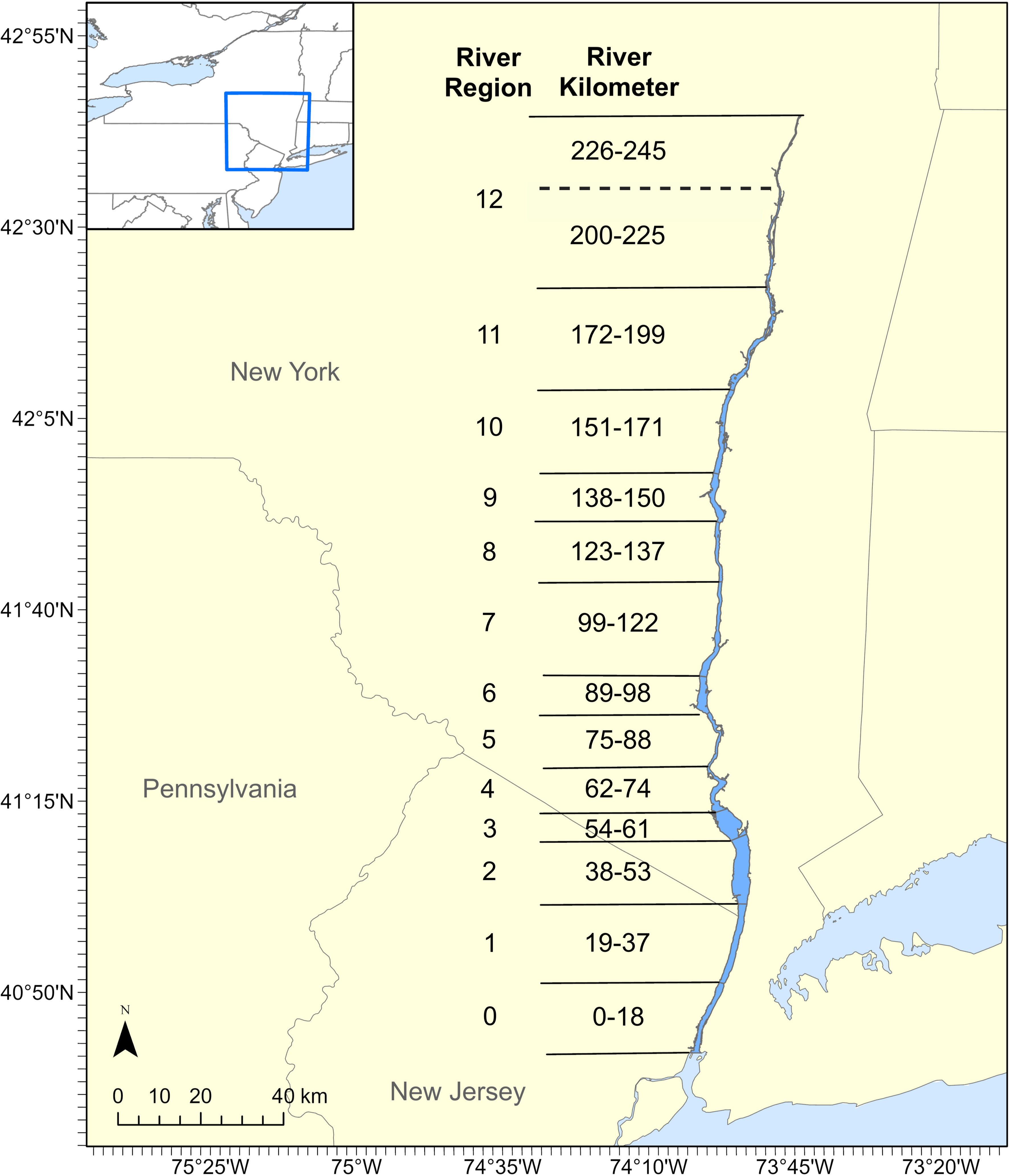
Figure 1 The Hudson River Estuary (in dark blue) divided into 13 river regions for the stratified random sampling design of the LRS based on river kilometer. The dashed line indicates the northernmost boundary of the study area prior to the expansion of the study area in 1988 when region 12 expanded to include river kilometers 226-245. Region 0 was not included in the sampling until 1988.

The Long River Ichthyoplankton Survey (LRS) under the Hudson River Biological Monitoring Program (HRBMP) is a fishery-independent ichthyoplankton trawl survey conducted continuously from 1974 through 2017. It was concluded in 2017 with the announcement of the closure of the Indian Point power plant. The LRS collected over 467 thousand observations for over 150 species in the HRE with over 108 thousand tows, targeting a range of fish species and providing critical information on the abundance and spatiotemporal distribution for their early life stages, including eggs, yolk-sac-larvae (YSL), post-yolk-sac-larvae (PYSL), young-of-year (YOY), and older. The LRS provided a unique opportunity to study how different fish species and fish communities respond to climatically and anthropogenically induced changes in environments within the HRE. However, before these data can be used they must be understood and their quality assured. While the LRS followed a stratified random survey design consistently over the survey period, many technical changes occurred during the survey to address various issues encountered in the survey due to logistic limitations, modified survey objectives, and foci on specific topics. These inconsistencies in sampling practices could introduce observation bias in the sampled fish abundance data, raising significant difficulties in using and interpreting survey catch rates and fish dynamics over space and time. This calls for a careful and comprehensive evaluation of the possible impacts of changing survey protocols and the development of approaches to calibrate and standardize the survey data to make them spatiotemporally consistent and comparable, serving as an excellent example for illustrating the process of calibrating fishery-independent data.

The present study aims to use the LRS as an example to develop a data calibration procedure and evaluate the impacts of sampling protocol changes on the estimates of fish abundances and spatiotemporal distributions. Using several representative species and their key early life stages, we aim to: 1) evaluate and identify the influential sampling factors to the LRS dataset, 2) explore appropriate and duplicable statistical approaches to calibrate the data to minimize the sampling bias in fish abundance indices and validate their performance, 3) provide more robust model-based abundance indices, and 4) demonstrate the risks of neglecting sampling bias by comparing discrepancies between the model-based abundance indices and the design-based abundance indices. The formulated data calibration procedure will be widely applicable to not only the entire LRS dataset but also similar fisheries surveys and biological monitoring programs seeking solutions to address sampling bias in data. The findings of this study will also provide insights into optimizing survey designs and analyzing survey data in broader environmental studies. These insights can contribute to improving the reliability and accuracy of abundance estimates in similar fishery-independent surveys.

2 Materials and methods

2.1 Long river survey

The HRE is the southern portion of the Hudson River, extending 245 rkm (river kilometer) from the Federal Dam in Troy, NY to the Battery in New York City (Figure 1). The upper portion of the HRE is a freshwater ecosystem and the southern 97 rkm is a brackish/marine ecosystem (Daniels et al., 2005). Although the sampling area covers from Albany to Battery Park, NY, the sampling in the Battery Park region and the northernmost reaches of the Albany region did not start until 1988.

The LRS ichthyoplankton data were collected throughout the HRE primarily from April through November, 1974-2017; however, the starting and ending dates varied from year to year (Figure 2). Sampling was done on a weekly basis during May-July, and on a biweekly basis during the other months. Although a stratum-based stratified random sampling design was used for determining sampling locations, the allocation of sampling effort across river regions and strata was adjusted over time based on the projected occurrence and spatial distribution of the target species and life stages (ASA Analysis & Communication (ASAAC), 2016). The sampling strata in the study are divided into 13 longitudinal river regions (Figure 1), ranging from Albany to Battery, and 3 habitat strata, including shoal, channel, and bottom (Heimbuch et al., 1992). A 1 m² Tucker trawl was used for sampling shoal and channel strata, and a 1 m² epibenthic sled was used for sampling the shoal and bottom strata. Both gears were fitted with 505 μm mesh plankton nets and were used for all sampling times and areas. In general, the Tucker trawl sampled shallower depths ranging from 0 to 47.3 meters (m) with a mean of 6.5 m, and the epibenthic sled sampled deeper depths ranging from 0 to 60.3 m with a mean of 10.57 m. The sample depth was the distance from the surface of the water to the top of the gear. The sample depth was determined randomly for each tow, based on the strata being sampled.

FIGURE 2

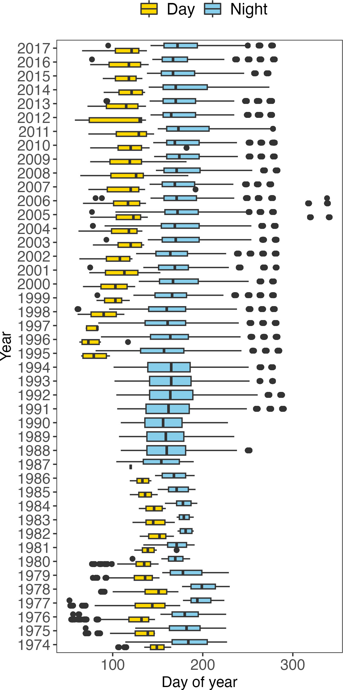
Figure 2 Boxplots of the sampling day of year for the Long River Survey in each year. The vertical bars in the boxes are medians. The left and right limits of the boxes are the first (Q1) and third (Q3) quartiles (25th and 75th percentiles). The difference between Q1 and Q3 is the interquartile range (IQR). Potential outliers are defined as observation points that fall outside the range of Q1-1.5*IQR and Q3 + 1.5*IQR. If potential outliers are presented, the whiskers extend to 1.5 times the IQR from Q1 or Q3. If no outliers are presented, the whiskers extend to the minima and maxima of the distributions. Yellow boxes denote daytime sampling, and navy-blue boxes denote nighttime sampling.

Sampling was carried out throughout the entire study area, during both daytime and nighttime except 1987-1994. Daytime was defined as the period from 30 minutes after sunrise to 30 minutes before sunset, while nighttime was defined as the period from 30 minutes after sunset to 30 minutes before sunrise. Prior to 1987, surveys were conducted in daylight until early June, after which they were conducted at night to minimize possible gear avoidance by the developing fish (Bowles et al., 1978; Boreman and Klauda, 1988). Gear avoidance by larval fish has been found to relate to visual stimuli (Bridger, 1956) and fish size, with larger fish exhibiting greater gear avoidance (Ahlstrom, 1954). Larval fish have been found to engage in diel migrations, (Haldorson et al., 1993; Murphy et al., 2011; Ospina-Alvarez et al., 2012), including species that are found in the HRE (Noble, 1970). From 1987 through 1994, no daytime sampling was conducted. Sampling intensity was heavily skewed toward nighttime from the years 2000 – 2017. The dates of switching from daytime to nighttime sampling were not consistent over the years (Figure 2).

Abundance data of ichthyoplankton and fishes at several life stages were collected from the LRS, including eggs, YSL, PYSL, and YOY. Analyses were performed using catch data for striped bass, white perch, and American shad (eggs, YSL, and PYSL), Atlantic tomcod (PYSL and YOY), and American eel (YOY and yearling and older (YROL).

2.2 Case study species

Five species were selected as species of focus with data from two or three life stages selected for each species for analysis (Table 1). These species and their respective life stages were selected considering their representation in the LRS database in terms of ecological roles, targeting status in the survey design, and socio-economic importance.

TABLE 1

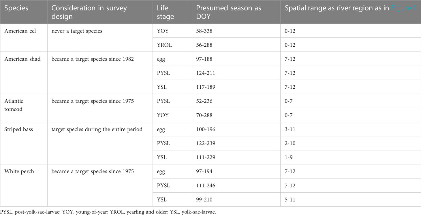
Table 1 Analyzed species and life stages selected from the Long River Survey database.

Striped bass is a significant species in the HRE not only because of their commercial value but also their iconic social-ecological importance (McLaren et al., 1988; Limburg et al., 2006). The Hudson River has been identified as a significant contributor of striped bass to the Atlantic coastal fisheries (McLaren et al., 1981), and the HRE is crucial spawning and nursery ground for striped bass (Nack et al., 2019). Striped bass were initially the single species of focus of the LRS because the utility company was obligated to demonstrate compliance with federal regulations for the construction and operation of the Cornwall pumped-storage facility and thermal power plants with once-through cooling (Barnthouse et al., 1988). Therefore, striped bass eggs, YSL, and PYSL were used in this study.

Later, the Federal Nuclear Regulatory Commission and the U.S. Environmental Protection Agency required the inclusion of white perch and Atlantic tomcod as Representative Important Species to define and assess their long-term population dynamics in relation to power plant operations (Barnthouse et al., 1988; Dew and Hecht, 1994b). The white perch and Atlantic tomcod were then included as target species in the LRS in 1975. Despite the closure of the white perch fishery due to PCB contamination in February 1976, white perch remain crucial in the HRE due to their abundant population, and the HRE serves as vital spawning and nursery grounds for them (Klauda et al., 1988a), thus white perch eggs, YSL, and PYSL were used. Atlantic tomcod stands out as the only abundant species that spawns during winter in the HRE. Their spawning grounds are mainly located in the lower Hudson River, which sets them apart from other fish species in the river in terms of their spatiotemporal distribution (Dew and Hecht, 1994a). Consequently, they are an important species to examine when assessing the impacts of changes on sampling protocols. Due to winter ice conditions in the river, the survey was not able to consistently sample the egg and YSL stages. Therefore, Atlantic tomcod PYSL and YOY stages were used in this study.

The Hudson River American shad fishery has a rich history in New York, existing for over 200 years and was one of the most profitable shad fisheries on the East Coast at one time, before the fishery closed in 2010 due to depletion of the stock (ASMFC (Atlantic States Marine Fisheries Commission), 2020). Despite the historical, economic and cultural importance of American shad, they did not become a target species in the survey until 1982. American shad are anadromous, relying on the HRE as their spawning and nursery habitat, therefore eggs, YSL, and PYSL were used in this study (Limburg, 1996a).

The Hudson River system accommodates several anadromous fish species that use it as a nursery habitat, yet American eel is the only catadromous fish found in the river, which renders them unique (Mattes, 1989). However, the LRS never intended to target the American eel, although the LRS data provided important stock assessment inputs for American eel juvenile and YROL life stages (ASMFC, 2017). Being a catadromous species, the larval eels migrate from the Sargasso Sea to the HRE after hatching, where they spend most of their lives in brackish or freshwater before returning to the Sargasso Sea to spawn (Schmidt, 1923; Mattes, 1989). Therefore, this study focused on American eels in older life stages (YOY and YROL). Additionally, the American eel is the most widely distributed fish species in the Hudson River system (Mattes, 1989), which makes it an excellent candidate for assessing the impact of changes in sampling protocols on non-target species.

2.3 Data calibration procedure

2.3.1 Variables selection

Changes in LRS sampling protocol had gone through variation in sampling timing in a day, sampling period in a year, sampling locations, gears, and depth. These changes could affect catch rates over the survey period for different species and hence were treated as predictors in our statistical modeling. We then used the catch-per-unit-effort (CPUE) of different species as the measurement of sampling efficiency, which was calculated by dividing the fish abundance by the filtered water volume in m³. Statistical modeling was built to describe the relationship between these variables with the following multivariate formula:

$\begin{array}{ll}CPUE\sim year+f(DOY)+f(hour)+f(rkm)+f(depth)+gear+f(op.inter.terms)+ϵ,& (1)\end{array}$

where CPUE is related to all the sampling protocol variables through their respective functions which are specified by different models. In this formula, CPUE denotes the CPUE value for certain species and life stage calculated from the LRS database, year denotes the data year, DOY denotes the sampling day of the year, hour denotes the sampling time of the day rounded to the hour, rkm denotes the sampling location measured with river kilometer, depth denotes the sampling depth, gear denotes the gear used in the records, and op.inter.terms denotes optional interaction terms between any variables that may be included in candidate models. Year and gear were modeled as discrete categorical variables while the other variables were modeled as continuous variables.

Multicollinearity among the predictors was evaluated using Variance Inflation Factor (VIF) analysis for all species and life stages prior to the model selection to avoid error inflation and unreliable coefficient estimates (Hair et al., 2010). Outliers in CPUE data were identified as those that were two times larger than the second largest value, which was then excluded from the model development process. As the LRS dataset did not record zero-catch tows from the survey for each species, we added zero-catch tows to the survey stations that did not have a catch record for the study species.

2.3.2 Candidate model exploration

We explored different statistical models to calibrate the catch rates for different species and life stages. We restricted our modeling to data collected from their habitats during the seasons each life stage occurred in the HRE, measured with the HRE river region and DOY, respectively (Table 1). The use of a stratum-based stratified random sampling design with 13 river regions by the LRS facilitates the description of the geographical distribution of a given species/life stage. The seasons of occurrence were determined as the ranges of DOY where the first and last non-zero catch was observed over the time series, and their spatial ranges were determined as the river regions they inhabit during certain life stages, through a literature review and preliminary data review. This design could not only ensure the calibrated survey catchability is ecologically reliable in terms of the species’ spatiotemporal dynamics but also reduce the potential bias in model fitting using maximum likelihood methods due to the “complete separation” issue (Albert and Anderson, 1984).

Specifically, the habitat of American shad was defined as the upper HRE (river region 7-12), according to their well-reported spawning activities (Limburg 1995; Limburg, 1996b). The occasional observations of American shad eggs in the lower HRE were assumed to be produced by vagrants from different river systems, indicated by their distinct otolith growth rates and Sr : Ca values (Limbrug, 1995), hence not included in our data calibration.

According to Klauda et al. (1988a) in their study on white perch, the upper zone of the freshwater area, particularly in the Saugerties-Albany regions, had a higher incidence of white perch spawning activity. The white perch eggs and YSL were similarly distributed spatially, as they have limited mobility and minimal downstream transport due to their short life stage duration (Klauda et al., 1988a). On the other hand, PYSL was more widely dispersed across the sampling regions in the upper and middle estuary zones (Klauda et al., 1988a). Therefore, for white perch eggs and YSL, the study area was limited to the upper HRE regions 7-12, while for PYSL, the study area was shifted to river regions 5-11.

Striped bass spawn mostly in the middle regions of the HRE (Boreman and Klauda, 1988), and they move downstream as they grow into larval stages (McLaren et al., 1981). This distributional shift by life stages was further adjusted and determined based on their occurrence. Atlantic tomcod is known as a winter spawner in the lower HRE (Klauda et al., 1988b). Accordingly, the inhabiting river regions for their PYSL and YOY were defined as the lower HRE (river regions 0-7) in this study. The American eel YOY and YROL habitats were defined as the entire HRE, considering that they were observed throughout the river, their well-developed mobility, and their catadromous nature (hatch in the ocean and enter the Hudson River Estuary at a later life stage) (Mattes, 1989). Although early life stages such as eggs and larvae are known to have limited mobility, the study areas were determined to cover a sufficient geographical range to include their distributions.

The LRS CPUE data were found to be heavily zero-inflated (Supplementary Materials Figure S-1), which is a common challenge in ecology statistical modeling that needs to be addressed with specified assumptions in distribution and model selections (Zuur et al., 2009). Recognizing the zero-inflated nature of the data, we conducted a preliminary model trial procedure with a suite of generalized models based on several different responsive variable assumptions that were widely used in modeling zero-inflated data in aquatic ecology. Following the standardized multivariate formula (1) and previous modeling practices (specified as references in the parenthesis), the trialed models included:

● Generalized Linear Models (GLMs) with negative binomial distribution (modeling fish abundance from catch sample data, Power and Moser, 1999);

● Generalized Additive Models (GAMs) with negative binomial distribution (modeling the Gulf of Mexico fish community abundance with climatic and oceanographic factors using a fishery-independent dataset, Drexler and Ainsworth, 2013);

● Generalized Additive Models (GAMs) with Tweedie distribution (modeling juvenile fish distribution with environmental variables and prey abundance in the Yellow Sea using a fishery-independent dataset, Xue et al., 2018);

● Generalized Additive Models (GAMs) with zero-inflated (hurdle) Poisson distribution (modeling juvenile crayfish river and stream habitats in New Zealand using an ecology survey database, Jowett et al., 2008);

● Generalized Additive Models (GAMs) with zero-inflated negative binomial distribution (modeling relative abundance indices of silky shark using data collected by observer programs, Lennert-Cody et al., 2019);

● Generalized Linear Models (GLMs) with zero-inflated negative binomial distribution (billfish CPUE standardization using commercial longline fishery data, Walsh and Brodziak, 2015);

● Generalized Linear Mixed-effects Models (GLMMs) with random intercept and slope (modeling Northwest Atlantic shark abundance using fishery-dependent data, Baum and Blanchard, 2010);

● Generalized Additive Mixed-effects Models (GAMMs) with random intercept and spline (modeling capability of two recreational species in West Australia using catch data, Navarro et al., 2020).

Considering some of the examined distributions were only applicable to discrete count data in ecology (such as negative binomial and Poisson distributions), we specifically modified the modeling techniques to deal with the continuous CPUE data in our study by incorporating offset terms (CPUE = catch.abundance/sampled.volume).

Despite these efforts, the preliminary model trial procedure showed that only the GAM assuming Tweedie distribution could return converged model outputs, while the other models either did not converge or returned extremely poor fitting with an R square of less than 0.01. Tweedie distribution is a generalization of several probability distributions including normal, gamma, inverse-Gaussian, and Poisson distribution, determined by a power parameter theta, which could be estimated via maximum likelihood estimation (Tweedie, 1984). With certain values of theta (1<theta<2), the Tweedie distribution can interpret a compound Poisson-gamma distribution (quasi-Poisson and quasi-negative binomial) in the response variable (Tweedie, 1984; Jørgensen, 1987). This characteristic makes it particularly effective in dealing with zero-inflated fisheries and aquatic data such as CPUE and catch volume (Shono, 2008; Arcuti et al., 2013; Berg et al., 2014). The GAMs with Tweedie distribution were developed with the R package “mgcv” version 1.8-40 (Wood and Wood, 2015).

2.3.3 Model selection

Three versions of Tweedie GAM variants were developed as the final candidate models following the multivariate formula (1), including a base version without optional interaction terms, a version with an interaction term between depth and year, and a version with an interaction term between depth and gear. The depth-year interaction was evaluated because the LRS tow depths were inconsistent over the surveyed year, with the tows from the more recent years concentrated in shallower water (Supplementary Materials Figure S-2). The depth-gear interaction was evaluated because the two survey gears (Tucker trawl and epibenthic sled) could have different selectivity by depth, which could result in misspecified catchability even in identical depths (Supplementary Materials Figure S-3).

The three final candidate models were developed for the case study species with their respective life stages. Among the candidate models, we aimed to select the single model that best described the survey catchability based on their goodness-of-fit, which were compared with three indicators: Akaike Information Criterion (AIC), Root Mean Square Error (RMSE), and deviance explained.

AIC is a widely used model selection criterion in ecological modeling (Portet, 2020). It measures the goodness-of-fit as well as model complexity of candidate models to a set of data based on the relationship between maximum likelihood and divergence, with a lower AIC value indicating a better fit. RMSE is a commonly used estimator in fisheries stock assessment to measure the difference between the model-fitted values $(\widehat{CPU{E}_t})$ and the observed value (CPUE_i) with the following equation (Wilberg and Bence, 2008; McCormick et al., 2012):

$\begin{array}{ll}RMSE= \sqrt{\frac{{\sum }_{i=1}^n{(CPU{E}_i- \widehat{CPU{E}_i})}^2}{n}}, & (2)\end{array}$

where n represents the number of CPUE observations. Deviance explained describes how much the fitted model can reduce the deviance compared to a null model that assumes no relationship between predictors and response variables. The values of deviance explained are always strictly between 0 to 1, with higher values representing better model fit.

2.3.4 Model validation

Two model validation procedures were implemented to evaluate the models’ predictive performance for different species and life stages, including a K-fold analysis and a retrospective analysis. The statistical analyses were conducted using R version 4.0.3 (R Core Team, 2020).

2.4 K-fold analysis

For the K-fold analysis, each dataset was divided into five equally sized subsets (folds). The data were randomly resampled within each year without replacement so each year of data is evenly represented in each of the five subsets. Cross-validation was then performed five times per model, with one subset used as a validation set, and the remaining four subsets combined and used as a training set. During each iteration, the model is trained on the training set and evaluated on the validation set.

To evaluate the models’ performance, RMSE, root relative square error (RRSE), and Spearman correlation coefficient estimated from each fold were used. The RMSE quantifies the average magnitude of the differences between predicted values and actual values. The RMSE indicates a perfect match between observed and predicted values when it equals zero, with higher RMSE values indicating an increasingly poor match (Kouadri et al., 2021).

The RRSE indicates how well a model performs relative to the average of the true values. Therefore, when the RRSE is lower than one, the model performs better than the simple model. Hence, the lower the RRSE, the better the model. The square root of the relative squared error is used to reduce the error to the same units as the predicted quantity (Kouadri et al., 2021):

$\begin{array}{ll}RRSE= \frac{\sqrt{{\sum }_{i=1}^n{(CPU{E}_i- \widehat{CPU{E}_i})}^2}}{\sqrt{{\sum }_{i=1}^n{(CPU{E}_i- \overline{CPUE})}^2}},& (3)\end{array}$

where$\overline{CPUE}$ denotes the mean observed CPUE value.

The correlation coefficient assesses the strength and direction of the monotonic relationship between the observations and predictions. Due to a large number of zeros and skewed distribution with extremely large values in the data, the Spearman correlation coefficient (rho) was used (Spearman, 1904).

2.5 Retrospective analysis

A retrospective analysis was performed by sequentially removing the data from the most recent years, fitting the best-fit models, and comparing the terminal year estimates (Kell et al., 2021). Retrospective analysis is widely used in quantitative fisheries science to understand the consistency of a statistical model’s performance over time, providing key diagnostic evidence for accepting or rejecting a model. The process of sequentially removing the last year’s data is called “peeling”. In this study, we performed a five-year peel for all the best-fit models and focused on the estimates of year-effects, as they represented the temporal trend in fish abundance, which was the most important stock status indicator. Specifically, we performed the peeling procedure by sequentially removing all data from the terminal year (2017) by a one-year step until five years (when 2012 became the terminal year). The model was then refitted with each set of truncated time series data using the same variable and model structure. We then compared the terminal year estimates of stock abundance to the full model estimate for that year for potential retrospective errors. We used a quantitative indicator, Mohn’s rho (Mohn, 1999), to measure the magnitude of the five-year retrospective errors, which is calculated as:

$\begin{array}{ll}Moh{n}^{\prime }s rho= \frac{1}{5} {\sum }_{t=T-5}^{T-1}\frac{y_{(1:t),t}- y_{(1:T),t}}{y_{(1:T),t}}& (4)\end{array}$

where T is the terminal year of the complete data series, t is the terminal year of the peeled data series, y_(1:t),t is the model-based year effect estimated for the terminal year using the peeled data series, y_(1:T),t and is the model-based year effect estimated for the terminal year using the full data series. Mohn’s rho ranges between -1 to 1, with a value close to 0 representing a negligible retrospective pattern in the model, indicating consistent model performance with different lengths of time-series data. According to the earlier simulation analyses based on integrated, age-structured models with different species (Hurtado-Ferro et al., 2015), a Mohn’s Rho is considered reflective of the existence of a retrospective pattern when its value is higher than 0.20 or lower than −0.15 for longer-lived species, or larger than 0.30 or lower than −0.22 for shorter-lived species, though these thresholds may not apply to age-aggregated CPUE estimates as in the presented study.

2.6 Model calibration effects

We measured the model calibration effects by comparing the model-based abundance indices (year effects estimated from the Tweedie GAMs) with the design-based abundance indices.

The design-based annual abundance indices have been historically used for evaluating fish abundances for key species. The design-based annual abundance indices (I) were calculated as averaged density (number of individuals divided by the volume of water sampled) over all surveyed regions, strata, and weeks (ASA Analysis & Communication (ASAAC), 2016):

$\begin{array}{ll}I={\sum }_{w=first week}^{last week}\left[\frac{{\sum }_{i=1}^{12}{\sum }_{s=1}^3{V}_{i,s}({\sum }_{j }^{}\frac{C{t}_{j,i,s,w}}{v_{j,i,s,w}})}{{\sum }_{i=1}^{12}{\sum }_{s=1}^3{V}_{i,s}}\right] & (5)\end{array}$

where Ct_j,i,s,w denotes the number of individuals of a species in sample j, region i, stratum s, and week w, v_j,i,s,w denotes the volume of water sampled for sample j in region i, stratum s, and week w, and V_i,s denotes the volume of stratum s in river region i, and first week denotes the first week of a year in which the accumulative weekly density estimates exceeds 5% of the sum of densities over all weeks of sampling, and last week is defined as first week + 7 weeks.

To make the annual abundance comparable over time, only river regions 1-12 were used as the Battery (river region 0) was not sampled until 1988. The weeks used for eggs, YSL, and PYSL of striped bass, American shad, and white perch were their proposed peak seasons, assuming an 8-week long duration of spawning season. For Atlantic Tomcod, due to ice conditions in the River, the LRS was unable to consistently sample the YSL stage. However, an abundance index for the period when the transformation from PYSL to the juvenile stage occurred could be calculated for weeks 19-22 (approximately DOY 127-154). This period roughly corresponds to the month of May, and the abundance of Age 0 tomcod was calculated from LRS data for these four weeks (ASA Analysis & Communication (ASAAC), 2016). The annual abundance of American eel was estimated based on data from weeks 18-26 when the survey was conducted throughout the river, assuming that the occurrence of YOY and YROL eels takes place during the spring and early summer (Mattes, 1989). To compare if the proposed weeks (PW) have effects on the estimates, we also estimate abundance indices using all weeks (AW). Pearson’s correlation coefficient was used to evaluate the correlation between design-based and model-based abundance indices (Shono, 2008).

Additional analyses were conducted for the Atlantic tomcod PYSL due to their unique spatiotemporal distribution. Although the Atlantic tomcod was included as a Representative Important Species in the survey in 1975 (Barnthouse et al., 1988), the allocation of sampling effort focused on the collection of Atlantic tomcod PYSL was discontinued in 1981 and was not resumed until 1995 (ASA Analysis & Communication (ASAAC), 1996). The missing allocation of sampling effort for tomcod as well as changing survey start dates (DOY) over the years (Figure 2) might have impacts on the estimates of PYSL abundance indices as the tomcod peak season for PYSL was reported from mid-March to mid-April (Klauda et al., 1988b). It is hypothesized that the abundance index would be negatively correlated with the survey start DOY as the early survey start DOY was more likely to include the peak season of tomcod PYSL, considering the survey started in late April or May that could have missed the peak season of high PYSL density. Furthermore, previous studies (Dew and Hecht, 1994a; Dew and Hecht, 1994b) indicated that a significant amount of tomcod 0-age abundance (29-45%) was not accounted for when the survey missed the seaward of the Yonkers region from March through May. Therefore, river regions 0-12 data collected from 1988 to 2017 were used to estimate design-based abundance indices for Atlantic tomcod PYSL and YOY using all weeks and proposed weeks to evaluate the potential impacts of exclusion of the Battery area. It is hypothesized that the inclusion of the Battery area data would improve the estimates of abundance indices, assuming a significant proportion of tomcod postlarvae and juveniles distributed in the Battery area (Klauda et al., 1988b; Dew and Hecht, 1994a; Dew and Hecht, 1994b).

The model-based abundance indices were denoted as I_M. The design-based abundance indices using the proposed weeks’ data were denoted as I_PW, and the design-based abundance indices using the proposed weeks’ data were denoted as I_AW for all species except for Atlantic tomcod PYSL. For the Atlantic tomcod PYSL, the design-based abundance indices using data with the inclusion of Battery area were denoted as I_{PW (0-12)} and I_{AW (0-12)}, and the design-based abundance indices using data without the inclusion of Battery area were denoted as I_{PW (1-12)} and I_{AW (1-12)}.

3 Results

3.1 Changes in sampling protocol

The changes in sampling protocol of the LRS have altered the catchability of different ichthyoplankton in the HRE. The duration of sampling varied yearly, with inconsistencies in the start and end dates (Figure 2). The number of days of sampling also varied, ranging from the 32 days of sampling in 1982 to 104 days of sampling in 1995. In addition to varying sampling duration, differences in diel timing of sampling fluctuated. Sampling during the day was conducted in the early weeks of the sampling season, for the years in which there was daytime sampling, starting as early as February and as late as May, and ending as early as March and as late as July (Figure 2). Nighttime sampling was conducted for later river runs, starting as early as February and as late as June, and ended as early as July and as late as October, with little overlap between daytime and nighttime sampling each year (Figure 2).

The Tucker trawl and epibenthic sled were inconsistently used throughout the LRS. The annual sampling intensity for the sled ranged from 270 tows in 2012 to 1591 tows in 1976, and for the trawl ranged from 982 tows in 1982 to 1974 tows in 1976 (Figure 3). The location of sampling also varied by year and by gear. The survey area expanded over the duration of the LRS (Figure 1) and the two gears were disproportionately used in different river regions. The differences in gear and sampling locations also resulted in changes in sampling depths throughout the LRS (Supplementary Materials Figure S-2).

FIGURE 3

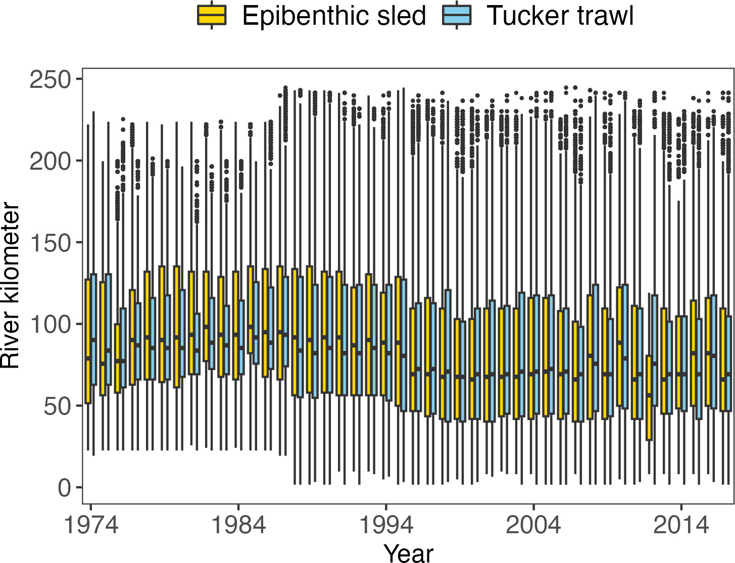
Figure 3 Boxplots of the usage of the two gears by river kilometer for all sampling tows for all species in each year of the LRS. The horizontal bars in the boxes are medians. The bottom and top limits of the boxes are the first (Q1) and third (Q3) quartiles (25th and 75th percentiles). The difference between Q1 and Q3 is the interquartile range (IQR). Potential outliers are defined as observation points that fall outside the range of Q1-1.5*IQR and Q3 + 1.5*IQR. If potential outliers are presented, the whiskers extend to 1.5 times the IQR from Q1 or Q3. If no outliers are presented, the whiskers extend to the minima and maxima of the distributions. Purple boxes denote sampling using an epibenthic sled, and green boxes denote sampling using a Tucker trawl.

3.2 Model fitting

Three versions of Tweedie GAM variants (a base version “tw.gam.base”, a version with depth and year interaction “tw.gam.depth.year”, and a version with depth and gear interaction “tw.gam.depth.gear”) were compared for their goodness-of-fit with AIC, deviance explained, and RMSE (Supplementary Materials Table S-1). The Tweedie GAM with depth and gear interaction performed the best among all cases (except for the Atlantic tomcod PYSL where it did not converge), exhibited particularly by AIC. The base model without interaction always had relatively higher AIC values and lower deviance explained and RMSE. However, the discrepancies in deviance explained and RMSE were mostly negligible. Considering the simplicity of base models and low computational demands (required less than 5% computation time given the large size of LRS), the base model demonstrated a more favorable tradeoff between model complexity and goodness of fit. Therefore, the base model was selected as the optimal calibration model for the following analyses.

Relationships between the survey CPUE and the six considered predictors were modeled using the base Tweedie GAM. The four spatio-temporal factors in the LRS were found to be strongly related to the predicted CPUE values for all species and life stages examined, and the year and gear effects were also significant (Supplementary Materials Figure S-4 to S-16). Peaks in DOY, hour, and Rkm were obvious and unsynchronized among species and life stages, indicating varied seasons and hours of appearance and use of habitat in the HRE. CPUE demonstrated fluctuations over the surveyed years, which could reflect model-based fish abundance (results and analysis see section 3.2). The epibenthic sled consistently displayed significantly higher median CPUE values compared to the Tucker trawl. In only 7 out of 13 cases did their CPUE distributions overlap, indicating considerable gear effects in survey catchability.

3.3 Model calibration effects

The model-based and design-based abundance indices were shown in Figure 4. The Pearson’s correlation coefficients (r) of the model-based and design-based abundance indices were all statistically significant for all species and life stages with a mean r of 0.76 except for Atlantic tomcod PYSL I_{AW (0-12)} and I_{AW (1-12)} (Figure 5 and Supplementary Materials Table S-2). The model-based and design-based abundance indices were generally highly correlated (r>0.73) for all species either using the PW data (see methods) or AW data except Atlantic tomcod.

FIGURE 4

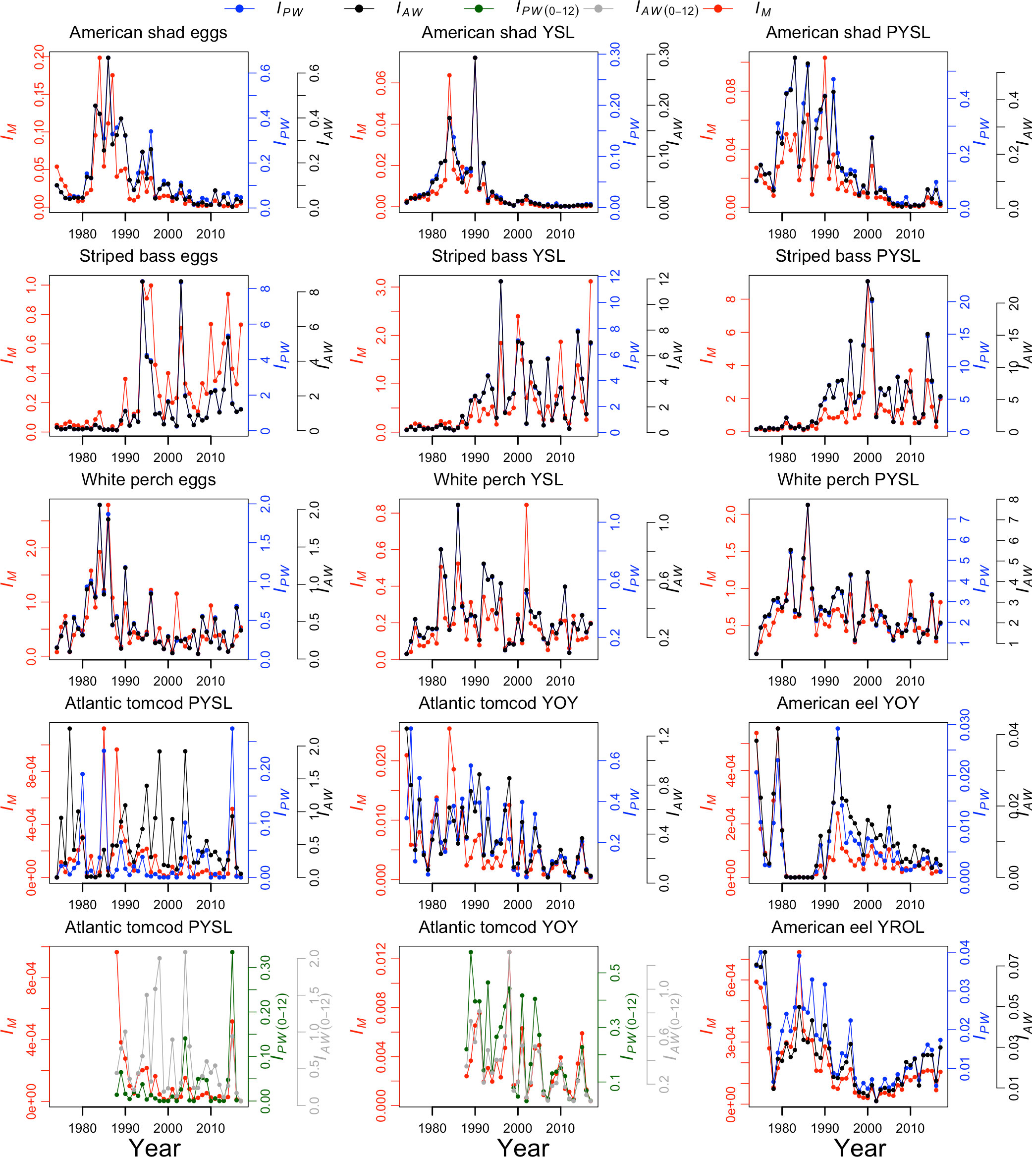
Figure 4 Model-based (I_M) and design-based abundance indices for each species and life stage. I_PW denotes the design-based abundance indices estimated using the proposed weeks’ data. I_AW denotes the design-based abundance indices estimated using all weeks’ data. For the Atlantic tomcod, the I_{PW (0-12)} denotes the design-based abundance indices estimated using proposed weeks data with the inclusion of Battery, and the I_{AW (0-12)} denotes the design-based abundance indices estimated using all weeks data with the inclusion of Battery. PYSL, post-yolk-sac-larvae; YOY, young-of-year; YROL, yearling and older; YSL, yolk-sac-larvae.

FIGURE 5

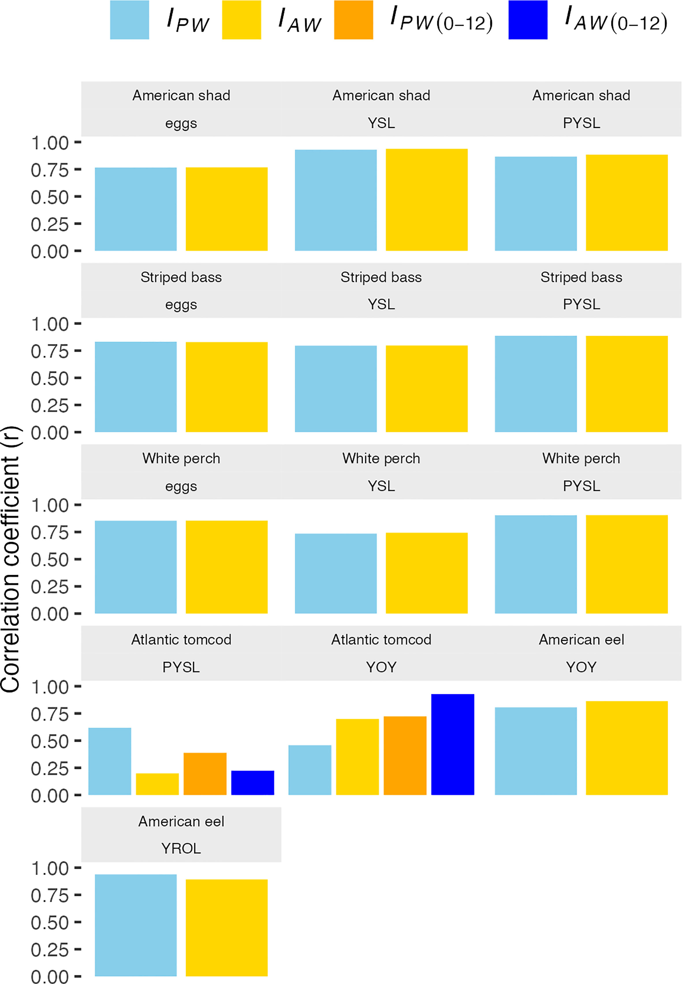
Figure 5 Pearson’s correlation coefficients between model-based and design-based abundance indices. I_PW denotes the design-based abundance indices estimated using the proposed weeks’ data. I_AW denotes the design-based abundance indices estimated using all weeks’ data. For the Atlantic tomcod, the I_{PW (0-12)} denotes the design-based abundance indices estimated using proposed weeks data with the inclusion of Battery, and the I_{AW (0-12)} denotes the design-based abundance indices estimated using all weeks data with the inclusion of Battery. PYSL, post-yolk-sac-larvae; YOY, young-of-year; YROL, yearling and older; YSL, yolk-sac-larvae.

The r of I_M and I_{PW (1-12)} was 0.62 (p<0.05, df=42) for tomcod PYSL; however, the r of I_M and I_{AW (1-12)} was only 0.20 (p=0.20, df=42). With the inclusion of the Battery river region data, the I_{PW (0-12)} still had a higher correlation coefficient with the I_M (r=0.39, p<0.05, df=28) than I_{AW (0-12)} (r=0.22, p=0.236, df=28). It should be noted that the estimates using inclusion and exclusion of the Battery data were not directly comparable as the inclusion of Battery data was only available from 1988-2017.

On the other hand, the r of I_M and I_{AW (1-12)} was 0.70 (p<0.05, df=42) for tomcod YOY; while the r reduced to 0.46 (p<0.05, df=42) for I_M and I_{PW (1-12)} (Table S-2). With the inclusion of the Battery data, the r of I_M and I_{PW (0-12)} for tomcod YOY was 0.72 (p<0.05, df=28) and the r of I_M and I_{AW (0-12)} for tomcod YOY was 0.93 (p<0.05, df=28).

Without the inclusion of the Battery data (1974-2017 time series), the I_{AW (1-12)} for tomcod PYSL was negatively correlated with survey start DOY (Figure 6A, r=-0.375, p<0.05, df=42) as hypothesized. The I_{PW (1-12)} was positively correlated with survey start DOY, although it was not statistically significant (Figure 6B, r=0.14, p=0.365, df=42). Similarly, the I_M (1974-2017) were positively correlated with survey start DOY (Figure 6C, r=0.331, p<0.05, df=42), reflecting declining abundance (Figures 3 and 4) when the survey started earlier and resumed the allocation of sampling effort for tomcod PYSL after 1995.

FIGURE 6

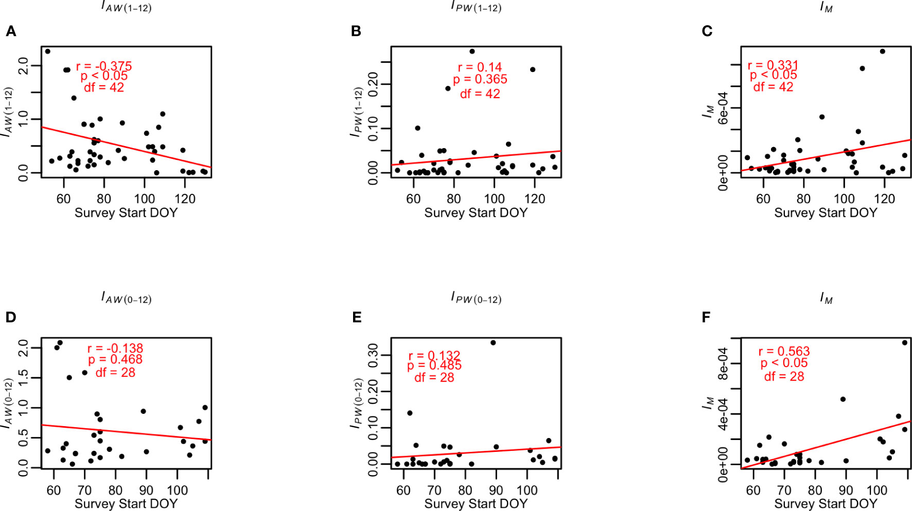
Figure 6 Relationships between (A) I_{AW (1-12)} and survey start DOY (day of year); (B) I_{PW (1-12)} and survey start DOY; (C) I_M and survey start DOY, using 1974-2017 time series, and (D) I_{AW (0-12)} and survey start DOY; (E) I_{PW (0-12)} and survey start DOY; and (F) I_M and survey start DOY using 1988-2017 time series data for the Atlantic tomcod PYSL. I_PW denotes the design-based abundance indices estimated using the proposed weeks’ data. I_AW denotes the design-based abundance indices estimated using all weeks’ data. I_{PW (0-12)} denotes the design-based abundance indices estimated using proposed weeks data with the inclusion of Battery, and the I_{AW (0-12)} denotes the design-based abundance indices estimated using all weeks data with the inclusion of Battery. A trendline using linear regression analysis was added to each of the panels, denoting the trend of the correlation.

With the Battery data (1988-2017 time series), the I_{PW (0-12)} and I_{AW (0-12)} were negatively (Figure 6D, r=-0.138, p=0.468, df=28) and positively (Figure 6E, r=0.132, p=0.485, df=28) correlated with survey start DOY, respectively, yet they were not statistically significant. The I_M (1988-2017) was still positively correlated with survey start DOY (Figure 6F, r=0.563, p<0.05, df=28).

3.4 Model validation

3.4.1 K-fold analysis

The RMSEs varied among species and life stages, depending on the statistics of each dataset. In general, the RMSEs estimated from the 5 trials generate similar RMSEs with low variation (Figure 7A and Supplementary Materials Table S-3). However, a few models (shad eggs and striped bass eggs) showed a wider range of RMSEs as the RMSE is sensitive to extreme values, reflecting the nature of the datasets. The rho between observations and predictions are all significantly different from zero at the significance level of 0.05, suggesting the observations and predictions are significantly correlated (rho around or higher than 0.5) (Figure 7B and Supplementary Materials Table S-3). However, the rho for eel YOY is notably lower (c. 0.25), possibly due to a lack of data during the 1980s. For most models, the RRSEs were below or around 1 (Figure 7C and Supplementary Materials Table S-3), suggesting reduced error compared to the simple models. Nevertheless, the RRSEs were above 1 for shad YSL and white perch eggs, indicating that the model performance was not satisfactory and caution should be taken for the accuracy of the estimates for these two models.

FIGURE 7

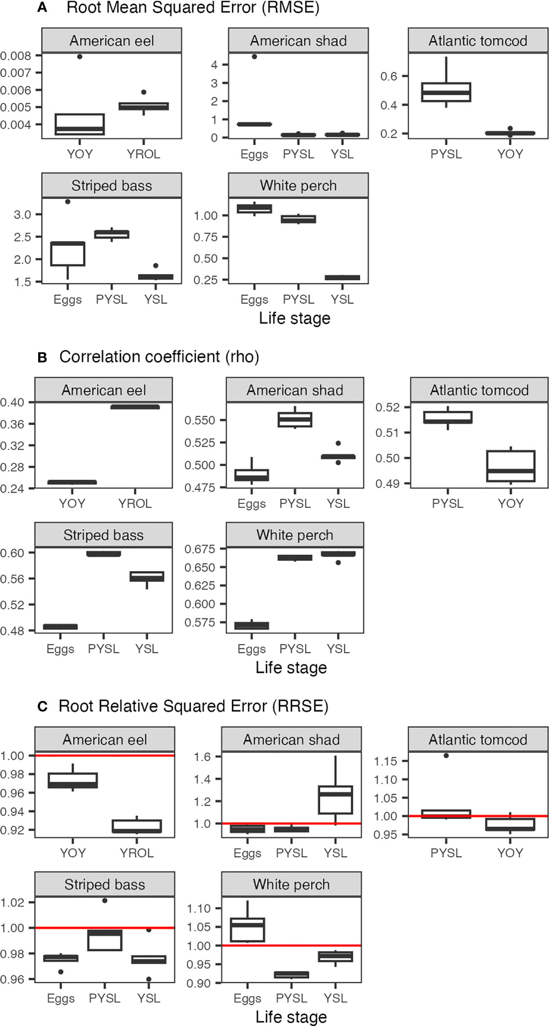
Figure 7 (A) Root mean squared error (RMSE); (B) Correlation coefficient (rho); and (C) Root relative squared error (RRSE) of the 5 folds for models of each species and life stage. The red lines indicate 1. PYSL, post-yolk-sac-larvae; YOY, young-of-year; YROL, yearling and older; YSL, yolk-sac-larvae. Note that the y-axis range differs among the panels.

3.4.2 Retrospective analysis

A five-year retrospective analysis indicated negligible retrospective errors in the optimal calibration model (base Tweedie GAMs) according to the estimated Mohn’s rho (Figure 8). The largest absolute value of Mohn’s rho was observed with “American shad egg” at 0.102, which did not indicate noticeable retrospective pattern (<0.3) for such a short-lived species. White perch had the smallest Mohn’s rho values for all its life stages compared with other examined species, indicating the most stable model fitting performance over time. Eggs tended to possess the largest absolute Mohn’s rho values compared with other life stages, implying a relatively stronger retrospective pattern in the optimal calibration model for egg abundance, despite their extremely low levels.

FIGURE 8

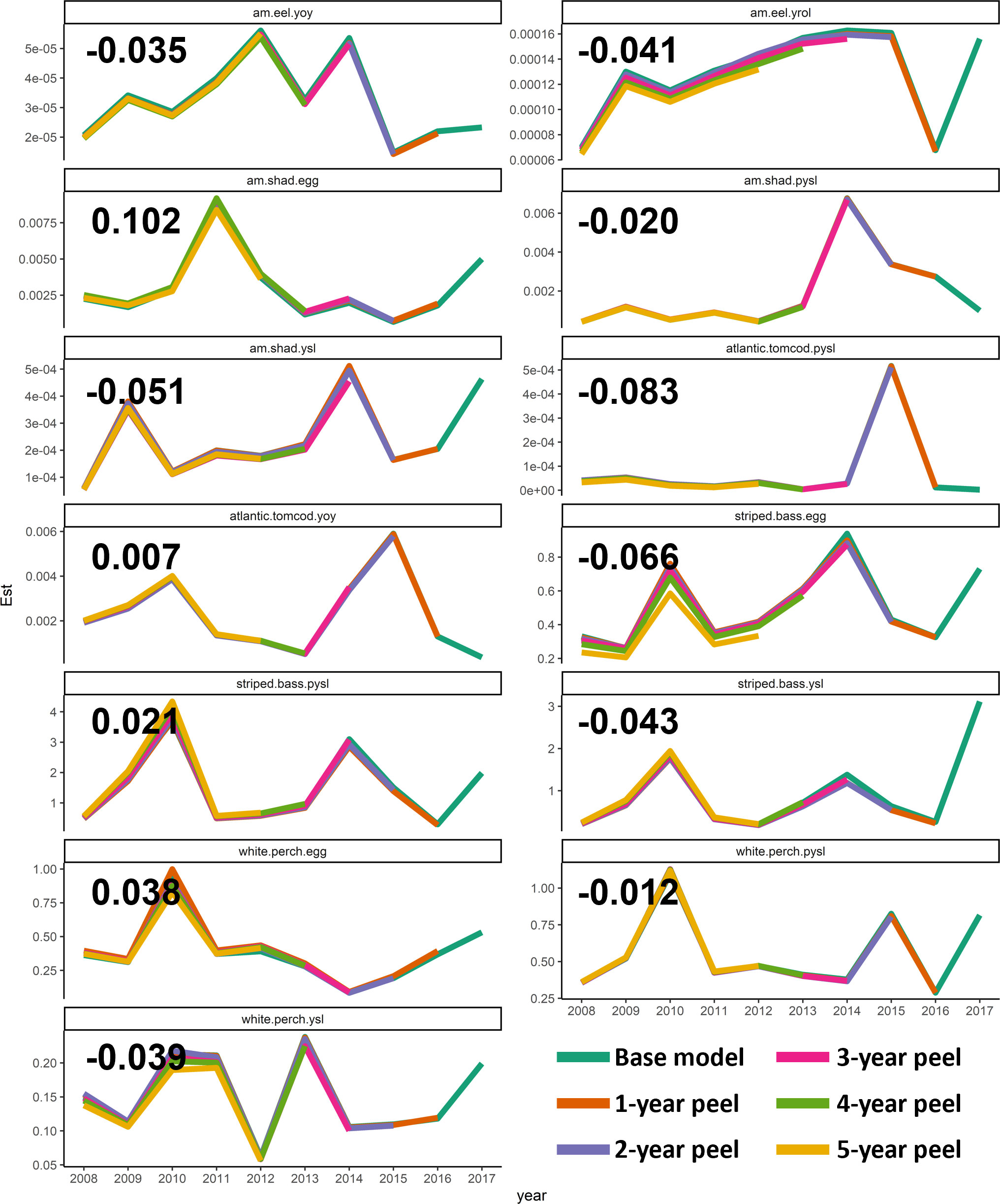
Figure 8 Retrospective trajectories of the year effects for the most recent 10 years for the optimal calibration model (The base Tweedie GAM). The calculated Mohn’s rho values are shown in the corresponding panel. Est represents the estimated CPUE value. PYSL, post-yolk-sac-larvae; YOY, young-of-year; YROL, yearling and older; YSL, yolk-sac-larvae.

While the retrospective patterns were not strong for the terminal years (based on which the Mohn’s rho values were estimated), there were still some retrospective patterns observed for the intermediate years. Specifically, variabilities between different “peel” models were observed around 2010 for striped bass egg, white perch egg, and white perch YSL. However, the relative range of these variabilities was always smaller than 15%, indicating low risks of retrospective patterns with the optimal calibration models.

4 Discussion

4.1 Model-based abundance indices can mitigate the spatiotemporal biases in design-based abundance indices

With the growing utilization of long-term data sets for establishing baseline reference points in aquatic environments, it becomes increasingly important to understand any biases or evaluate the uncertainty that may arise from changes in sampling strategies or protocols (Tuckey and Fabrizio, 2013). In this study, the model-based and design-based abundance indices generally exhibited high correlation, despite inconsistencies in the sampling protocol across various areas and time periods resulting in some unsampled areas and inconsistent survey durations and shifts between day and night. This suggests that the design-based abundance indices provide valuable information that is comparable to the model-based abundance indices, even without accounting for sampling effects resulting from changes in the protocol, when considering the annual and river-wide scale.

However, abundance can be underestimated or overestimated when important factors were not considered (e.g., peak season, major spatial distribution). The model-based abundance indices take these factors (e.g., spatial and temporal variables) into account and can address the inconsistent sampling issue. Furthermore, the model estimated sampling effects reflected the observations in other studies. For example, the model estimated the two spatial peaks for striped bass eggs around rkm 90 and rkm 140 (Supplementary Materials Figure S-11), which corresponded to the observations in Boreman and Klauda (1988). Also, even with the inconsistent survey start DOY, the model estimated the highest density of Atlantic tomcod PYSL occurred during DOY 70-120 (Supplementary Materials Figure S-9), which corresponded to the observations in previous studies (Klauda et al., 1988b; Dew and Hecht, 1994a). On the contrary, the design-based indices may be sensitive to the inconsistent allocation of sampling effort over space and time, especially for early life stages. If the peak of spawning for eggs and YSL occurs in a specific location and time, it can be challenging to capture the maximum abundance of these life stages both spatially and temporally, especially since they last for less than a week (Boreman and Klauda, 1988). The Atlantic tomcod illustrated an example that the estimates could be considerably affected by the inconsistent sampling protocol.

Dew and Hecht (1994a; 1994b) pointed out that it is necessary to include the most seaward region of the estuary (Battery) to define a self-contained, measurable population of larval and early juvenile Atlantic tomcod. Our results showed that the inclusion of the Battery region did improve the estimates of abundance for tomcod YOY, suggesting that there is a considerable amount of Atlantic tomcod juveniles distributed in the Battery area over the season. However, the estimates of abundance with the inclusion of Battery may still be biased for the tomcod PYSL if the peak season was missed in several years. In other words, even if the majority of the spatial distribution of the population was covered by the survey, the inconsistent sampling protocol would still have significant impacts on the estimates of abundance if the peak season was missed in several years, especially for early life stages that generally have sharp seasons. Timing in relation to the seasonal cycle and location of the target species, and the fact that only a limited amount of data can be collected, are considered to be two main deficiencies in fishery-independent surveys, which could lead to unrepresentative sampling (Hilborn and Walters, 1992; Pennino et al., 2016). The Atlantic tomcod in this study provides an example where the estimates derived from the fishery-independent survey could be biased.

Although abundance indices were used for evaluating changes in annual abundance for each species, especially for early life stages due to their high mortality rates, it should be noted that having more accurate absolute abundance estimates can provide valuable insights and benefits for fisheries management. Absolute abundance estimates provide information on the size and productivity of the population, which is crucial for setting appropriate fishing quotas or catch limits. Reliable abundance estimates contribute to more effective and sustainable management practices. Furthermore, absolute abundance estimates could be used to identify threatened or endangered populations (e.g. sturgeon species), monitoring population recovery efforts, and assessing the effectiveness of conservation measures. While relative indices provide useful information for assessments, having more accurate absolute abundance estimates adds value from a management perspective.

4.2 Sampling efficiencies on the target and non-target species

Long-term fishery-independent survey datasets often involve the addition of new target species, which may require modifications to the sampling protocol. However, the effects of these changes on both target and non-target species are often overlooked, even though data from non-target species can offer valuable insights into population dynamics and ecosystem dynamics. The design-based abundance indices for the eggs and larval stages of most target species (striped bass, American shad, and white perch) included in this study showed a strong correlation with the model-based abundance indices, whether using all weeks or only the proposed week data. This could be due to the fact that early life stages of fishes tend to have shorter seasons compared to juvenile and older stages (Boreman and Klauda, 1988), and the assumption of the design-based abundance indices that the periods of early life stages present in the river last seven weeks seemed reasonable for the three target species (Heimbuch et al., 1992) when estimating annual abundance indices.

Although both white perch and Atlantic tomcod were included as Representative Important Species since 1975 due to their high abundance and susceptibility to impingement and entrainment (Barnthouse et al., 1988; Klauda et al., 1988a), there was no allocation of sampling effort for tomcod during 1981-1994. The exact reason for over ten years of discontinuation of sampling allocation for the Atlantic tomcod was not clear. It is possibly because of the unique spatiotemporal distribution of the Atlantic tomcod as the only abundant winter spawners in the lower HRE, making it different from other target species (Dew and Hecht, 1994a). This, however, suggests that being considered as a target species did not guarantee better data quality compared to non-target species, particularly when the sampling events were not carried out consistently. As suggested by Dew and Hecht (1994a), a sampling plan that is designed to capture other major species in the Hudson River may not be optimal for the Atlantic tomcod due to its unique characteristics.

On the contrary, the abundance indices of American eel showed high correlations (r > 0.8, p< 0.05, df = 42) between the I_AW and I_PW with I_M. Despite never being a target species in the LRS, this finding suggested that the survey had adequately covered the major spatiotemporal distributions of American eel YOY and YROL in most years, even with the changing sampling protocol. However, during the 1980s, several years had no catch data for American eel YOY (1982-1987 and 1990), and only two YOY were observed in 1984, making it challenging to evaluate the effect of survey start date on the abundance index estimates, given that most early survey start dates occurred in the 1980s (Figure 2). It is unclear whether American eel YOY were not observed or were not considered in the survey during those years, as American eel was not regarded as a target species in the LRS.

4.3 Spatiotemporal effects in data calibration

For long-term fishery-independent surveys, spatiotemporal scales can be an important factor for assessing the accuracy and uncertainty associated with the estimates. The impact of changes in sampling protocol on estimates varies depending on the scale and purpose of the analysis, as shown in this study. When examining annual and river-wide trends, the design-based abundance indices for most species were consistent with model-based abundance indices, indicating that the major spatiotemporal distributions were well captured by the survey and that the sampling protocol changes did not significantly affect the estimates. However, when analyzing spatiotemporal changes at a finer scale, estimates may be biased or incomparable over time. For instance, the onset of the spawning season for American shad could not be accurately estimated in some years due to a late start in the survey. Additionally, when evaluating distributional shifts over time, the sampling location effects must be taken into account, as some areas were not sampled in early years, which could bias the estimates, especially for species distributed in both ends of the survey area (Dew and Hecht, 1994a; Dew and Hecht, 1994b). Although this study considered several significant factors, there may be other potential factors that can influence the estimates, such as variations in the spawning season due to the lunar phase (Takemura et al., 2004) or climate-related environmental changes (O’Connor et al., 2012). Similarly, distributional shifts over time may be caused by factors such as water quality changes, habitat alterations, invasive species, and anthropogenic activities, which are beyond the scope of this study and require further investigation.

4.4 Implications for future survey data calibration and sampling design

This study highlights the importance of identifying target species when designing fishery-independent surveys, as they determine the necessary spatiotemporal coverage of the survey. The results derived from this study indicate that the survey should sufficiently cover the significant spatiotemporal distributions of the target species. This study emphasizes how sampling protocol changes could result in biased estimates of abundance indices (e.g. Atlantic tomcod), providing valuable insights for future sampling protocols. Additionally, the model-estimated spatiotemporal distributions for each species and life stage provide critical information for designing future sampling allocations.

The calibration models developed in this study were effective in removing the effects not directly related to abundance and accounting for changes in the sampling protocol over time. The employed Tweedie GAMs can produce robust data calibration effects with different sample sizes and lengths of time-series data according to the retrospective analysis. However, for a few species and life stages, the uncertainty of the estimates should be taken with caution. For example, the shad YSL and white perch eggs models’ performance were not satisfactory, suggesting that there may be other important variables that were not included in the models driving the changes in CPUEs. On the contrary, the retrospective analysis showed that the developed calibration model performed consistently with different lengths of time-series survey data, indicating a relatively stable catchability pattern over the historical years. The K-fold analyses also showed satisfactory prediction performance for most species and life stages, demonstrating relatively consistent calibration effects over varying sample sizes. However, a calibration model update is still required when extreme climatic or environmental events are observed in the HRE ecosystem, as they may drastically affect the spawning dynamics of ichthyoplankton and result in altered survey efficiency.

Some caveats should be noted when interpreting the prediction results over the calibration models. First, the LRS did not have a cross-design sampling scheme which could generate full combinations of all sampling variables at all levels. This could disallow the use of mixed-effect models that assume nested design in data sampling (Schielzeth and Nakagawa, 2013) and result in limitations in predicting the sampling catchability over space and time, although these variables were treated as continuous variables (Webster et al., 2020). In most years, the daytime sampling started first in the year and switched to nighttime sampling to reduce gear avoidance by the PYSL (Boreman and Klauda, 1988), while each species and life stage have varying spawning and growth schedules. Furthermore, there was no or very limited daytime sampling during 1987-1994. Therefore, it should be noted that the daytime and nighttime effects on CPUE might be an artifact resulting from the sampling protocol. Second, the nature of the LRS data poses additional challenges in modeling and predicting sampling catchability. Specifically, the records on ichthyoplankton juvenile abundance (measured with “count”) are often in decimal numbers as they were expanded from subsamples collected for laboratory processes, which is a common and standard procedure in collecting juvenile surveys. The dominance of zero tows further adds to the complexity of the data distribution and they appear with various sampling efforts (measured with “water volume filtered”). We chose to use CPUE as an abundance index for the data calibration based on Tweedie GAM, which was the only option that could best address these data issues. However, the smoothing effects in the GAMs still could not perfectly predict the zero CPUE value, which limited its predictive power for extremely low and high catch scenarios.

The identified effects in the sampling designs not only can provide a baseline to calibrate the historical LRS dataset but also offer valuable insights for developing and optimizing future survey designs. The statistical patterns in the sampling factors (such as sampling season, time, and location) highlight improved or reduced survey efficiencies for different species as well as life stages in the HRE. This knowledge allows for more effective sampling for species with emphasized conservation or management demands, while a tradeoff still exists between species-specific and whole-community levels survey objectives. To ensure better data calibration quality, it is recommended to conduct some more standardized samplings following a strict cross-design. This will generate comparable catch records in terms of sampling design and hence enable the evaluation of relative catch efficiencies using more statistical approaches. Gaining a thorough understanding of how to apply available data sets and recognizing their limitations will provide valuable support to scientists and managers who are confronted with uncertainties in research surveys and are tasked with the challenge of effectively managing resources.

Data availability statement

The original contributions presented in the study are included in the article/Supplementary Material. Further inquiries can be directed to the corresponding author/s.

Author contributions

Conceptualization: H-YC, MS, KR, YC. Literature review: H-YC, MS, KR. Design and methodology: H-YC, MS, KR, YC. Statistical analysis and interpretation: H-YC, MS. Writing-original draft preparation: H-YC, MS, KR. Writing-review and editing: H-YC, MS, KR, YC. Supervision and securing funds: YC. All authors contributed to the article and approved the submitted version.

Funding

This study was funded by a Hudson River Foundation research grant (B01/22A).

Acknowledgments

We express our gratitude to Patrick Sullivan, Gregg Kenney, Richard Pendleton, John Maniscalco, and the NYSDEC and Hudson River Foundation staff for their valuable inputs and discussions. The HRBMP data have been generously gifted to Stony Brook University by the Entergy Corporation. We also extend our appreciation to all those who have contributed to the HRBMP throughout the years.

Conflict of interest

The authors declare that the research was conducted in the absence of any commercial or financial relationships that could be construed as a potential conflict of interest.

Publisher’s note

All claims expressed in this article are solely those of the authors and do not necessarily represent those of their affiliated organizations, or those of the publisher, the editors and the reviewers. Any product that may be evaluated in this article, or claim that may be made by its manufacturer, is not guaranteed or endorsed by the publisher.

Supplementary material

The Supplementary Material for this article can be found online at: https://www.frontiersin.org/articles/10.3389/fmars.2023.1237549/full#supplementary-material

References

Ahlstrom E. H. (1954). Distribution and abundance of egg and larval populations of the Pacific Sardine. Fishery. Bull. 56, 83–140.

Google Scholar

Albert A., Anderson J. A. (1984). On the existence of maximum likelihood estimates in logistic regression models. Biometrika 71 (1), 1–10. doi: 10.1093/biomet/71.1.1

CrossRef Full Text | Google Scholar

Arcuti S., Calculli C., Pollice A., D’Onghia G., Maiorano P., Tursi A. (2013). Spatio-temporal modelling of zero-inflated deep-sea shrimp data by Tweedie generalized additive. Statistica 73 (1), 87–101. doi: 10.6092/issn.1973-2201/3987

CrossRef Full Text | Google Scholar

ASA Analysis & Communication (ASAAC). (1996). 1995 year class report for the Hudson river estuary monitoring program (Marlboro, NY, USA: Prepared for Entergy Nuclear Operations, Inc).

Google Scholar

ASA Analysis & Communication (ASAAC). (2016). 2016 year class report for the Hudson river estuary monitoring program (Marlboro, NY, USA: Prepared for Entergy Nuclear Operations, Inc).

Google Scholar

ASMFC (Atlantic States Marine Fisheries Commission). (2017). American Eel Stock Assessment Update (Arlington, VA: ASMFC), 123.

Google Scholar

ASMFC (Atlantic States Marine Fisheries Commission). (2020). American shad benchmark stock assessment and peer review report (Arlington, VA: ASMFC), 1208.

Google Scholar

Barnthouse L. W., Klauda R. J., Vaughn D. S. (1988). What We Didn’t Learn about the Hudson River, Why, and What it Means for Environmental Assessment. Am. Fisheries. Soc. Monograph. 4, 329–335.

Google Scholar

Baum J. K., Blanchard W. (2010). Inferring shark population trends from generalized linear mixed models of pelagic longline catch and effort data. Fisheries. Res. 102 (3), 229–239. doi: 10.1016/j.fishres.2009.11.006

CrossRef Full Text | Google Scholar

Berg C. W., Nielsen A., Kristensen K. (2014). Evaluation of alternative age-based methods for estimating relative abundance from survey data in relation to assessment models. Fisheries. Res. 151, 91–99. doi: 10.1016/j.fishres.2013.10.005

CrossRef Full Text | Google Scholar

Boreman J., Klauda R. J. (1988). Distributions of early life stages of striped bass in the Hudson River estuary 1974-1979. Am. Fisheries. Soc. Monograph. 4, 53–58.

Google Scholar

Bowles R. R., Merriner J. V., Grant G. C. (1978). Factors associated with accuracy in sampling fish eggs and larvae (Washington, DC: Fish and Wildlife Service of US).

Google Scholar

Bridger J. P. (1956). On day and night variation in catches of fish larvae. Ices. J. Mar. Sci. 22 (1), 42–57. doi: 10.1093/icesjms/22.1.42

CrossRef Full Text | Google Scholar

Chiarini M., Guicciardi S., Angelini S., Tuck I. D., Grilli F., Penna P., et al. (2022). Accounting for environmental and fishery management factors when standardizing CPUE data from a scientific survey: A case study for Nephrops norvegicus in the Pomo Pits area (Central Adriatic Sea). PloS One 17, e0270703. doi: 10.1371/journal.pone.0270703

PubMed Abstract | CrossRef Full Text | Google Scholar

Cooper J. C., Cantelmo F. R., Newton C. E. (1988). Overview of the Hudson river estuary. Am. Fish. Soc Monogr. 4, 11–24.

Google Scholar

Daniels R. A., Limburg K. E., Schmidt R. E., Strayer D. L., Chambers R. C. (2005). “Changes in fish assemblages in the tidal Hudson River, New York,” in Historical changes in large river fish assemblages of the Americas. Eds. Rinne J. N., Hughes R. M., Calamusso B. (Bethesda, Maryland: American Fisheries Society), 471–504.

Google Scholar

Dew C. B., Hecht J. H. (1994a). Hatching, estuarine transport, and distribution of larval and early juvenile Atlantic tomcod, Microgadus tomcod, in the Hudson River. Estuaries 17, 472–488. doi: 10.2307/1352677

CrossRef Full Text | Google Scholar

Dew C. B., Hecht J. H. (1994b). Recruitment, growth, mortality, and biomass production of larval and early juvenile Atlantic tomcod in the Hudson River Estuary. Trans. Am. Fisheries. Soc. 123, 681–702. doi: 10.1577/1548-8659(1994)123<0681:RGMABP>2.3.CO;2

CrossRef Full Text | Google Scholar

Drexler M., Ainsworth C. H. (2013). Generalized additive models used to predict species abundance in the Gulf of Mexico: an ecosystem modeling tool. PloS One 8 (5), e64458. doi: 10.1371/journal.pone.0064458

PubMed Abstract | CrossRef Full Text | Google Scholar

Ducharme-Barth N. D., Grüss A., Vincent M. T., Kiyofuji H., Aoki Y., Pilling G., et al. (2022). Impacts of fisheries-dependent spatial sampling patterns on catch-per-unit-effort standardization: A simulation study and fishery application. Fisheries. Res. 246, 106169. doi: 10.1016/j.fishres.2021.106169

CrossRef Full Text | Google Scholar

Hair J. F., Anderson R. E., Babin B. J., Black W. C. (2010). Multivariate Data Analysis: A Global Perspective (7th Edition). Upper Saddle River. New Jersey: Pearson, 816

Google Scholar

Haldorson L., Prichett M. A., Paul A. L., Ziemann D. A. (1993). Vertical distribution and migration of fish larvae in a Northeast Pacific bay. Mar. Ecol. Prog. Ser. 101, 67–80. doi: 10.3354/meps101067

CrossRef Full Text | Google Scholar

Harley S. J., Myers R. A., Dunn A. (2001). Is catch-per-unit-effort proportional to abundance? Can. J. Fish. Aquat. Sci. 58, 1760–1772. doi: 10.1139/cjfas-58-9-1760

CrossRef Full Text | Google Scholar

Heimbuch D. G., Dunning D. J., Young J. R. (1992). “Post-yolk sac larvae abundance as an index of year class strength of striped bass in the Hudson River,” in Estuarine research in the 1980s. Ed. Smith C. L. (Albany, N.Y: SUNY Press), 376–391.

Google Scholar

Hilborn R., Walters C. J. (1992). Quantitative fisheries stock assessment: Choice, dynamics, & uncertainty (New York: Chapman and Hall), 570.

Google Scholar

Hurtado-Ferro F., Szuwalski C. S., Valero J. L., Anderson S. C., Cunningham C. J., Johnson K. F., et al. (2015). Looking in the rear-view mirror: bias and retrospective patterns in integrated, age-structured stock assessment models. ICES. J. Mar. Sci. 72 (1), 99–110. doi: 10.1093/icesjms/fsu198

CrossRef Full Text | Google Scholar

Jørgensen B. (1987). Exponential dispersion models. J. R. Stat. Soc.: Ser. B. (Methodological). 49 (2), 127–145. doi: 10.1111/j.2517-6161.1987.tb01685.x

CrossRef Full Text | Google Scholar

Jowett I. G., Parkyn S. M., Richardson J. (2008). Habitat characteristics of crayfish (Paranephrops planifrons) in New Zealand streams using generalised additive models (GAMs). Hydrobiologia 596, 353–365. doi: 10.1007/s10750-007-9108-z

CrossRef Full Text | Google Scholar

Kell L. T., Sharma R., Kitakado T., Winker H., Mosqueira I., Cardinale M., et al. (2021). Validation of stock assessment methods: is it me or my model talking? ICES. J. Mar. Sci. 78 (6), 2244–2255. doi: 10.1093/icesjms/fsab104

CrossRef Full Text | Google Scholar

Klauda R. J., McLaren J. B., Schmidt R. E., Dey W. P. (1988a). Life history of white perch in the Hudson River estuary. Amer. Fish. Soc. Monogr. 4, 69–88.

Google Scholar

Klauda R. J., Moos R. E., Schmidt R. E. (1988b). Life History of Atlantic Tomcod, Microgadus tomcod, in the Hudson River Estuary, with Emphasis on Spatio-Temporal Distribution and. Fisheries research in the Hudson River. (Albany, New York, USA: SUNY Press), 219.

Google Scholar

Kouadri S., Elbeltagi A., Islam A. R. M., Kateb S.. (2021). Performance of machine learning methods in predicting water quality index based on irregular data set: application on Illizi region (Algerian southeast). Appl. Water Sci. 11, 1–20. doi: 10.1007/s13201-021-01528-9

CrossRef Full Text | Google Scholar

Lennert-Cody C. E., Clarke S. C., Aires-da-Silva A., Maunder M. N., Franks P. J. S., Román M., et al. (2019). The importance of environment and life stage on interpretation of silky shark relative abundance indices for the equatorial Pacific Ocean. Fish. Oceanogr. 28, 1–11. doi: 10.1111/fog.12385

CrossRef Full Text | Google Scholar

Levinton J. S., Waldman J. R. (2006). The Hudson river estuary (Cambridge: Cambridge University Press).

Google Scholar

Limbrug K. E. (1995). Otolith strontium traces environmental history of subyearling American shad Alosa sapidissima. Mar. Ecol. Prog. Ser. 119, 25–35. doi: 10.3354/meps119025

CrossRef Full Text | Google Scholar

Limburg K. E. (1996a). Modelling the ecological constraints on growth and movement of juvenile American shad (Alosa sapidissima) in the Hudson River estuary. Estuaries 19, 794–813. doi: 10.2307/1352298

CrossRef Full Text | Google Scholar

Limburg K. E. (1996b). Growth and migration of 0-year American shad (Alosa sapidissima) in the Hudson River estuary: otolith microstructural analysis. Can. J. Fish. Aquat. Sci. 53, 220–238. doi: 10.1139/f95-160

CrossRef Full Text | Google Scholar

Limburg K., Hattala K., Kahnle A., Waldman J. (2006). “Fisheries of the Hudson river estuary,” in The Hudson river estuary. Eds. Levinton J., Waldman J. (Cambridge: Cambridge University Press), 189–204. doi: 10.1017/CBO9780511550539.016

CrossRef Full Text | Google Scholar

Mattes K. C. (1989). The ecology of the American eel, Anguilla rostrata (LeSueur), in the Hudson River (New York, USA: Fordham University).

Google Scholar

Maunder M. N., Thorson J. T., Xu H., Oliveros-Ramos R., Hoyle S. D., Tremblay-Boyer L., et al. (2020). The need for spatio-temporal modeling to determine catch-per-unit effort based indices of abundance and associated composition data for inclusion in stock assessment models. Fish. Res. 229, 105594. doi: 10.1016/j.fishres.2020.105594

CrossRef Full Text | Google Scholar

McCormick J. L., Quist M. C., Schill D. J. (2012). Effect of survey design and catch rate estimation on total catch estimates in Chinook Salmon fisheries. North Am. J. Fisheries. Manage. 32 (6), 1090–1101. doi: 10.1080/02755947.2012.716017

CrossRef Full Text | Google Scholar

McLaren J. B., Cooper J. C., Hoff T. B., Lander V. (1981). Movements of Hudson River striped bass. Trans. Am. Fisheries. Soc. 110 (1), 158–167. doi: 10.1577/1548-8659(1981)110<158:MOHRSB>2.0.CO;2

CrossRef Full Text | Google Scholar

McLaren J. B., Klauda R. J., Hoff T. B., Gardinier M. (1988). “Commercial fishery for striped bass in the Hudson river 1931-80,” in Fisheries research in the Hudson river. Ed. Smith C. L. (Albany: State University of New York Press), 89–123.

Google Scholar

Mohn R. (1999). The retrospective problem in sequential population analysis: an investigation using cod fishery and simulated data. ICES. J. Mar. Sci. 56 (4), 473–488. doi: 10.1006/jmsc.1999.0481

CrossRef Full Text | Google Scholar

Murphy H., Jenkins G., Hamer P., Swearer S. (2011). Diel vertical migration related to foraging success in snapper Chrysophys auratus larvae. Mar. Ecol. Prog. Ser. 433, 185–194. doi: 10.3354/meps09179

CrossRef Full Text | Google Scholar

Nack C. C., Swaney D. P., Limburg K. E. (2019). Historical and projected changes in spawning phenologies of American shad and striped bass in the Hudson River Estuary. Mar. Coast. Fisheries. 11 (3), 271–284. doi: 10.1002/mcf2.10076

CrossRef Full Text | Google Scholar

Navarro M., Hailu A., Langlois T., Ryan K. L., Kragt M. E. (2020). Determining spatial patterns in recreational catch data: a comparison of generalized additive mixed models and boosted regression trees. ICES. J. Mar. Sci. 77 (6), 2216–2225. doi: 10.1093/icesjms/fsz123

CrossRef Full Text | Google Scholar

Noble R. L. (1970). Evaluation of the Miller High-Speed Sampler for sampling yellow perch and walleye fry. J. Fisheries. Res. Board. Canada. 27 (6), 1033–1044. doi: 10.1139/f70-119

CrossRef Full Text | Google Scholar

O’Connor M. P., Juanes F., McGarigal K., Gaurin S. (2012). Findings on American Shad and striped bass in the Hudson River Estuary: a fish community study of the long-term effects of local hydrology and regional climate change. Mar. Coast. Fisheries. 4 (1), 327–336. doi: 10.1080/19425120.2012.675970

CrossRef Full Text | Google Scholar

Ospina-Alvarez A., Parada C., Palomera I. (2012). Vertical migration effects on the dispersion and recruitment of European anchovy larvae: From spawning to nursery areas. Ecol. Model. 231, 65–79. doi: 10.1016/j.ecolmodel.2012.02.001

CrossRef Full Text | Google Scholar

Pennino M. G., Conesa D., Lo ípez-Qu íılez A., Muñoz F., Fernaíndez A., Bellido J. M. (2016). Fishery-dependent and -independent data lead to consistent estimations of essential habitats. ICES. J. Mar. Sci. 73, 2302–2310. doi: 10.1093/icesjms/fsw062

CrossRef Full Text | Google Scholar

Portet S. (2020). A primer on model selection using the Akaike Information Criterion. Infect. Dis. Model. 5, 111–128. doi: 10.1016/j.idm.2019.12.010

CrossRef Full Text | Google Scholar

Power J. H., Moser E. B. (1999). Linear model analysis of net catch data using the negative binomial distribution. Can. J. Fisheries. Aquat. Sci. 56 (2), 191–200. doi: 10.1139/f98-150

CrossRef Full Text | Google Scholar

R Core Team (2020). R: A language and environment for statistical computing (Vienna, Austria: R Foundation for Statistical Computing). Available at: https://www.R-project.org/.

Google Scholar

Schielzeth H., Nakagawa S. (2013). Nested by design: model fitting and interpretation in a mixed model era. Methods Ecol. Evol. 4 (1), 14–24. doi: 10.1111/j.2041-210x.2012.00251.x

CrossRef Full Text | Google Scholar

Schmidt J. (1923). The breeding places of the eel. Philos. Trans. R. Soc Lond. B. Biol. Scl. 211, 179–208.

Google Scholar

Shono H. (2008). Application of the Tweedie distribution to zero-catch data in CPUE analysis. Fisheries. Res. 93 (1-2), 154–162. doi: 10.1016/j.fishres.2008.03.006

CrossRef Full Text | Google Scholar

Spearman C. (1904). The proof and measurement of association between two things. Am. J. Psychol. 15 (1), 72–101. doi: 10.2307/1412159.JSTOR1412159

CrossRef Full Text | Google Scholar

Takemura A., Rahman M. S., Nakamura S., Park Y. J., Takano K. (2004). Lunar cycles and reproductive activity in reef fishes with particular attention to rabbitfishes. Fish. Fisheries. 5 (4), 317–328. doi: 10.1111/j.1467-2679.2004.00164.x

CrossRef Full Text | Google Scholar

Tuckey T. D., Fabrizio M. C. (2013). Influence of survey design on fish assemblages: implications from a study in chesapeake bay tributaries. Trans. Am. Fisheries. Soc. 142, 957–973. doi: 10.1080/00028487.2013.788555

CrossRef Full Text | Google Scholar

Tweedie M. C. (1984). “An index which distinguishes between some important exponential families,” in Statistics: Applications and new directions: Proc. Indian statistical institute golden Jubilee International conference. (Calcutta, India: is Indian Statistical Institute), 579, 579–604.

Google Scholar

Walsh W. A., Brodziak J. (2015). Billfish CPUE standardization in Hawaii longline fishery: Model selection and multimodel inference. Fisheries. Res. 166, 151–162. doi: 10.1016/j.fishres.2014.07.015

CrossRef Full Text | Google Scholar

Walters C. (2003). Folly and fantasy in the analysis of spatial catch rate data. Can. J. Fish. Aquat. Sci. 60, 1433–1436. doi: 10.1139/f03-152

CrossRef Full Text | Google Scholar

Webster R. A., Soderlund E., Dykstra C. L., Stewart I. J. (2020). Monitoring change in a dynamic environment: spatiotemporal modelling of calibrated data from different types of fisheries surveys of Pacific halibut. Can. J. Fisheries. Aquat. Sci. 77 (8), 1421–1432. doi: 10.1139/cjfas-2019-0240

CrossRef Full Text | Google Scholar

Wilberg M. J., Bence J. R. (2008). Performance of deviance information criterion model selection in statistical catch-at-age analysis. Fisheries. Res. 93 (1-2), 212–221. doi: 10.1016/j.fishres.2008.04.010

CrossRef Full Text | Google Scholar

Wood S., Wood M. S. (2015). Package ‘mgcv’. R Package version. 1 (29), 729.

Google Scholar

Xue Y., Tanaka K., Yu H., Chen Y., Guan L., Li Z., et al. (2018). Using a new framework of two-phase generalized additive models to incorporate prey abundance in spatial distribution models of juvenile slender lizardfish in Haizhou Bay, China. Mar. Biol. Res. 14 (5), 508–523. doi: 10.1080/17451000.2018.1447673

CrossRef Full Text | Google Scholar

Zuur A. F., Ieno E. N., Walker N. J., Saveliev A. A., Smith G. M. (2009). Mixed effects models and extensions in ecology with R Vol. 574 (New York: springer), 574.

Google Scholar