Different vertical heat transport induced by submesoscale motions in the shelf and open sea of the northwestern South China Sea

Submesoscale currents are known to be associated with strong vertical velocities (O (10) m/day), regulating the redistributions of energy and matter balances. The northern South China Sea (SCS) is fulfilled with submesoscale motions, which might induce strong vertical heat transport (VHT). We set up a 1-km horizontal resolution Massachusetts Institute of Technology General Circulation Model (MITgcm) to study the seasonal variations in submesoscale vertical heat transport in shelf regions and open seas. Spectrum analysis shows that the spatial scale separating submesoscale and mesoscale motions are 14 and 30 km for the shelf and open regions, respectively. The submesoscale VHT in the shelf region is one order of magnitude larger than that in the open ocean. The former has the largest value in summer and winter, which might be induced by summer upwelling and winter downwelling, while the latter is strongest in winter and weakest in summer in open regions. The submesoscale VHT also appears to have intra-seasonal variations and might be attributed to the disturbances of tropical cyclones and life stages of submesoscale eddies. The submesoscale VHT is strongest in the pregeneration phase of the eddies, and the maximum VHT belt has an entrainment type at the developing and mature stages. The chlorophyll-a concentration also has the same temporal variation as the different life-stage of eddies. This study provides local VHT induced by submesoscale motions, which is expected to improve our understanding of submesoscale air–sea interactions and their biological effects.

1 Introduction

The spatial scale of submesoscale processes is approximately O (0.1–10) km, and the temporal scale is approximately O (0.1–1) day (McWilliams, 2016; Jing et al., 2020). They are widely distributed in the upper ocean and represent a type of motion between mesoscale motions and turbulent dissipation, playing an important role in the energy cascade of oceanic motions of different scales (Capet et al., 2008a). Submesoscale processes are accompanied by strong vertical motions, with vertical velocities one order of magnitude higher than those induced by mesoscale processes (Klein and Lapeyre, 2009). This determines their important role in processes such as heat budget, momentum exchange, and nutrient transport in the upper ocean (Capet et al., 2008b; Omand et al., 2015; Brannigan, 2016; Zhong et al., 2017; Su et al., 2018).

Vertical heat transport (VHT) is one of the key mechanisms regulating the climate of the ocean (Siegelman et al., 2020) and plays an important role in processes such as ocean–atmosphere interactions (Liu et al., 2018), polar climate change (Nummelin et al., 2017), and global warming (Yang et al., 2018). The VHT induced by submesoscale processes is an important component of global heat transport (Su et al., 2020b). In the active regions of submesoscale processes, the VHT induced by them is much greater than that caused by mesoscale processes (Large and Yeager, 2009; Siegelman, 2020; Su et al., 2020b), exerting a significant influence on the absorption of oceanic heat (Bachman et al., 2017; Siegelman et al., 2020). The study of submesoscale VHT is of great significance for more accurate estimation of the ocean’s heat storage capacity (Siegelman et al., 2020) and for improving the accuracy of atmospheric–oceanic model simulations (Liu et al., 2010).

Since 2000, numerical models have been widely applied to submesoscale process research (Dong and Zhong, 2018). Thanks to improvements in resolution and parameterization, numerical simulation has become an important tool for studying submesoscale processes. Qiu et al. (2014) used OGCM for the Earth Simulator (OFES) model data to study the characteristics of submesoscale eddies along the North Pacific Subtropical Countercurrent. Dong et al. (2021) found that symmetric instability in the upper mixed layer has obvious regional dependence and seasonal variation characteristics using LLC4320 model data. Cao and Jing (2022) discovered strong submesoscale processes below the mixed layer in the northwestern Pacific Ocean using the ROMS model and discussed their unique features, mechanisms, and impacts on the mixed layer, which are different from those in the mixed layer. For the South China Sea (SCS), many scholars have utilized numerical simulations to discuss the physical phenomena, dynamic mechanisms, spatial distribution, and temporal variation of submesoscale processes (Dong and Zhong, 2018; Cao et al., 2022; Jiang et al., 2022; Jiang et al., 2023; Li et al., 2019; Zhang et al., 2020a), deepening the understanding of submesoscale processes in the SCS.

Submesoscale processes have been observed in the SCS. Zhong et al. (2017) conducted high-resolution observations on an anticyclonic eddy in the northern SCS, obtaining a more detailed three-dimensional structure of submesoscale features at the eddy front and analyzing their mechanisms and intensities. Qiu et al. (2019) observed a submesoscale front at the edge of a warm eddy using underwater gliders. Tang et al. (2023) observed submesoscale processes in a severe wind event in the western SCS using a high-frequency float (Navis-SL1). Zhang and Qiu (2020) discovered spiral-banded submesoscale structures penetrating into the center of mesoscale eddies using satellite color remote sensing, altimetry, and drifting buoy data. Dong and Zhong (2020) found that submesoscale temperature fronts frequently appear on the northern shelf of the SCS in winter. Qiu et al. (2022a) analyzed the spatiotemporal distribution characteristics of submesoscale ageostrophic motion in the SCS using altimetry and surface drifting buoy data and pointed out that its spatiotemporal scale could become a good indicator for submesoscale eddy-resolving models. In addition to satellite remote sensing and in-situ observations, submesoscale processes can also be obtained through high-frequency Doppler radar (Yoo et al., 2018), seismic reflection profiles (Yang et al., 2022), and other methods. The kinetic energy of submesoscale processes is strongest in winter and weakest in summer (Zhong et al., 2017) and may be induced by mesoscale geostrophic straining (Qiu et al., 2022a) or strong wind events (Tang et al., 2023).

Submesoscale processes generate large vertical velocities, which can transfer heat from colder, deeper layers to warmer surface layers, contributing significantly to the overall VHT. Su et al. (2018) and Su et al. (2020b) used data from the LLC4320 model to study submesoscale processes at different frequencies and found that the average VHT caused by low-frequency (<f, where $f$ is the inertial oscillation frequency) submesoscale processes in the upper ocean in winter at mid-latitudes reaches 100 W/m², which is comparable to the air–sea heat flux. On the other hand, the global integral of high-frequency submesoscale VHT in winter reaches about 7 PW, greatly enhancing the total amount of vertical heat transport in the global ocean. Siegelman (2020) suggested that submesoscale VHT occurs not only in the upper ocean but also in the ocean interior. In the Antarctic Circumpolar Current (ACC) region, deep submesoscale fronts can transport heat upward from the ocean interior. This result is consistent with in-situ measurements by Siegelman et al. (2020) and Yu et al. (2019), which have demonstrated strong positive submesoscale vertical heat transport in the ocean interior. In contrast to studying a particular region using an Eulerian coordinate system, Wang et al. (2022) focused on submesoscale VHT controlled by mesoscale eddies and found that it exhibits rapid positive and negative spatial changes in eddy centers and their vicinity but shows upward heat transport after averaging over the region.

Previous studies have also investigated submesoscale VHT in the SCS. Zhang et al. (2020b) used OFES model data to investigate the spatiotemporal characteristics of submesoscale VHT in the SCS and found that it shows a strong winter-spring and weak summer-autumn seasonal distribution pattern, as well as a strong offshore and island-peripheral distribution and a weak inner area distribution. Zheng and Jing (2022) focused on submesoscale VHT in submesoscale filaments in the northern SCS and found that there is a secondary vertical circulation in eddy regions, accompanied by vertical heat fluxes up to 110 W/m².

Influenced by factors such as the intrusion of the Kuroshio Current, monsoon variations, and complex topography, SCS has complex multiscale dynamic processes (Dong and Zhong, 2018; Zheng et al., 2020). The southeastern Hainan Island in the northwestern SCS has a narrow and steep continental slope (Shu et al., 2018), and it is a typical shelf-slope region. Upwelling occurs frequently in this area in the summer (Xie et al., 2012), while downwelling occurs frequently in the winter (Jing et al., 2015). There are abundant frontal processes all year (Jing et al., 2015; Chen and Hu, 2023). At the same time, some mesoscale eddies invade the continental slope of this sea with greater energy and strain rates (Su et al., 2020a; Qiu et al., 2022b). All these factors provide favorable conditions for submesoscale processes. Therefore, exploring the characteristics of submesoscale VHT in the northwestern SCS is of great significance for understanding ocean–atmosphere heat exchange in shelf-slope regions and revealing their environmental effects. However, the difference in submesoscale VHT between shelf and open water is still unclear. Therefore, this study will focus on submesoscale VHT in the shelf and open water of northwestern SCS and explore its characteristics and possible mechanisms.

2 Data and methods

2.1 Data

2.1.1 Satellite data

The level-2 sea surface temperature (SST) product measured by the Visible and Infrared Imager/Radiometer Suite (VIIRS) sensor of the Suomi-NPP satellite from June to July 2020 is used to validate the numerical model. It has a spatial resolution of 0.75 km and a temporal resolution of 1 h. The access website is https://ncc.nesdis.noaa.gov/NOAA-20/NOAA20VIIRS.php.

Another SST product is obtained from the Operational Sea Surface Temperature and Sea Ice Analysis (OSTIA) system, which has a 5-km spatial resolution and daily temporal resolution (https://ghrsst-pp.metoffice.gov.uk/ostia-website/index.html). The products are merged with microwave and infrared satellite SSTs provided by the Group for the High-Resolution Sea Surface Temperature project (Martin et al., 2012).

Daily sea-level anomaly (SLA) with a spatial resolution of 0.25° is obtained from the Archiving, Validation, and Interpretation of Satellite Oceanographic data (AVISO) project, which integrates JASON-1, TOPEX/Poseidon, and ERS-1/ERS-2 products (https://www.aviso.altimetry.fr/en/data/data-access.html).

The level-2 chlorophyll-a concentration products are obtained from the VIIRS onboard the JPSS-1. The spatial resolution of these data is about 0.75 km, and the temporal resolution is several hours.

2.1.2 High-resolution nested simulation data

We set up the Massachusetts Institute of Technology General Circulation Model (MITgcm) to investigate submesoscale structures. To reduce the influence of the open boundaries in the simulation area as much as possible and to improve the computational efficiency, we run MITgcm using a rectangular one-way nested grid with two levels. MITgcm adopts the z-coordinate and static approximation because, for submesoscale flow of ${\text{R}}_o\approx 1$, the vertical scale in the upper ocean is much smaller than the horizontal scale, that is, $\text{H}/\text{L }\ll 1$.

The bathymetric chart is derived from ETOPO1 provided by the National Oceanic and Atmospheric Administration, which is an arc-minute global relief model of the Earth’s surface. As shown in Figure 1, the parent grid named M1 covers a spatial range of 100°E–135°E and 0°N–30°N with a horizontal resolution of 0.25°. The initial conditions of M1 are based on the January climatological data of WOA2018 (https://www.nodc.noaa.gov/cgi-bin/OC5/woa18/woa18.pl). The boundary conditions, sea surface relaxation, and wind field are all interpolated using SODA3 (http://apdrc.soest.hawaii.edu/erddap/search/index.html?page=1&itemsPerPage=1000&searchFor=soda). After 15 years of spin-up, the temperature, salinity, and major currents of the SCS reach statistically steady states.

FIGURE 1

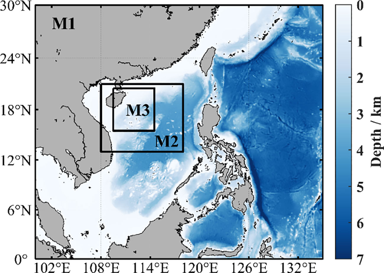
Figure 1 The model domain and bathymetry. The largest area, M1 (resolution: 25 km), covers 100°E–135°E and 0°N–30°N. The larger black box is M2 (resolution: 5 km), which covers 108°E–118°E and 13°N–21°N. The smallest black box is M3 (resolution: 1 km), which covers 109.5°E–114.5°E and 15.5°N–20.5°N.

Based on the results of the M1 climatological state, the nested zone M2 covering 108°E–118°E and 13°N–21°N in the northern SCS is selected for one-way nesting with a horizontal resolution of 0.05°. The M2 boundary conditions are from HYCOM gofs3.1 daily data (https://www.hycom.org/dataserver/gofs-3pt1/analysis), and the initial conditions are from the climatological data of M1. The wind field and other meteorological data for calculating the sea surface heat flux are interpolated from the ERA5 reanalysis data provided by the European Center for Medium-Range Weather Forecasts (https://www.ecmwf.int/en/forecasts/datasets). The simulation period is from 1 October 2017 to 31 July 2020.

The horizontal resolution of M3 (15.5°N–20.5°N, 109.5°E–114.5°E) is refined to 0.01° (about 1 km). The boundary conditions of M3 are provided by the M2 output data, including temperature, salinity, velocity, and sea surface height. The K-profile parameterization (Large et al., 1994) is adopted for parameterizing vertical mixing. The M3 simulation spans from 1 August 2019 to 31 July 2020, with 6-hourly outputs of sea surface height, temperature, salinity, and velocity. The time step is 100 s.

2.1.3 Validation of the model data

It is necessary to examine the accuracy of the model data before using them. The simulated annual average SST image is compared with OSTIA SST and the simulated annual average velocity image with AVISO products. As shown in Figures 2A, B, the model reproduces the cyclonic circulation in the north of the SCS, and the velocity and range of the SCSWBC have a similar spatial distribution with AVISO. However, the simulated velocity at the southwest boundary and the southeast boundary is different from that of AVISO, which may be due to the influence of the flow correction at the boundary of the model on the simulation results.

FIGURE 2

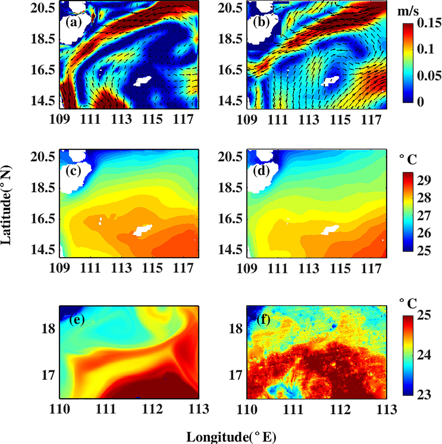
Figure 2 Comparison between MITgcm and satellite observations. The top panels show the mean surface velocity from (A) M2 simulated data and (B) AVISO data. The middle panels are the mean sea surface temperature distribution of (C) M2 simulated data and (D) OSTIA data. The bottom panels are the sea surface temperature of (E) M3 simulated data and (F) VIIR images at 06:00 on 6 February 2020.

The simulated annual average SST is higher in the southeastern corner of the analysis region, which is consistent with the spatial distribution of OSTIA SST (Figures 2C, D). A submesoscale front (~10 km) observed by VIIRS satellite data on 6 February 2020 is also captured by MITgcm (Figures 2E, F). In general, it is found that the output of MITgcm is reliable and meets the research needs of submesoscale motions.

We also validate the seasonal variations of modeled temperatures and velocities. Figure 3 shows the seasonal variation of temperatures at 5, 55, and 110m. The spatial distribution of temperatures is consistent between SODA3 and MITgcm in all seasons. The fine structures of MITgcm are much clearer than those of SODA3. The mean biases of temperature in spring, summer, autumn, and winter are −0.15°C, 0.10°C, 0.19°C, and 0.18°C, respectively. Figure 4 shows the seasonal variation of the velocities of SODA3 and MITgcm. Although the modeled magnitudes of velocity are lower than the observed value in the four seasons, the main current, i.e., the western boundary current, is significant in both the SODA3 and MITgcm. It indicates our model result is reliable.

FIGURE 3

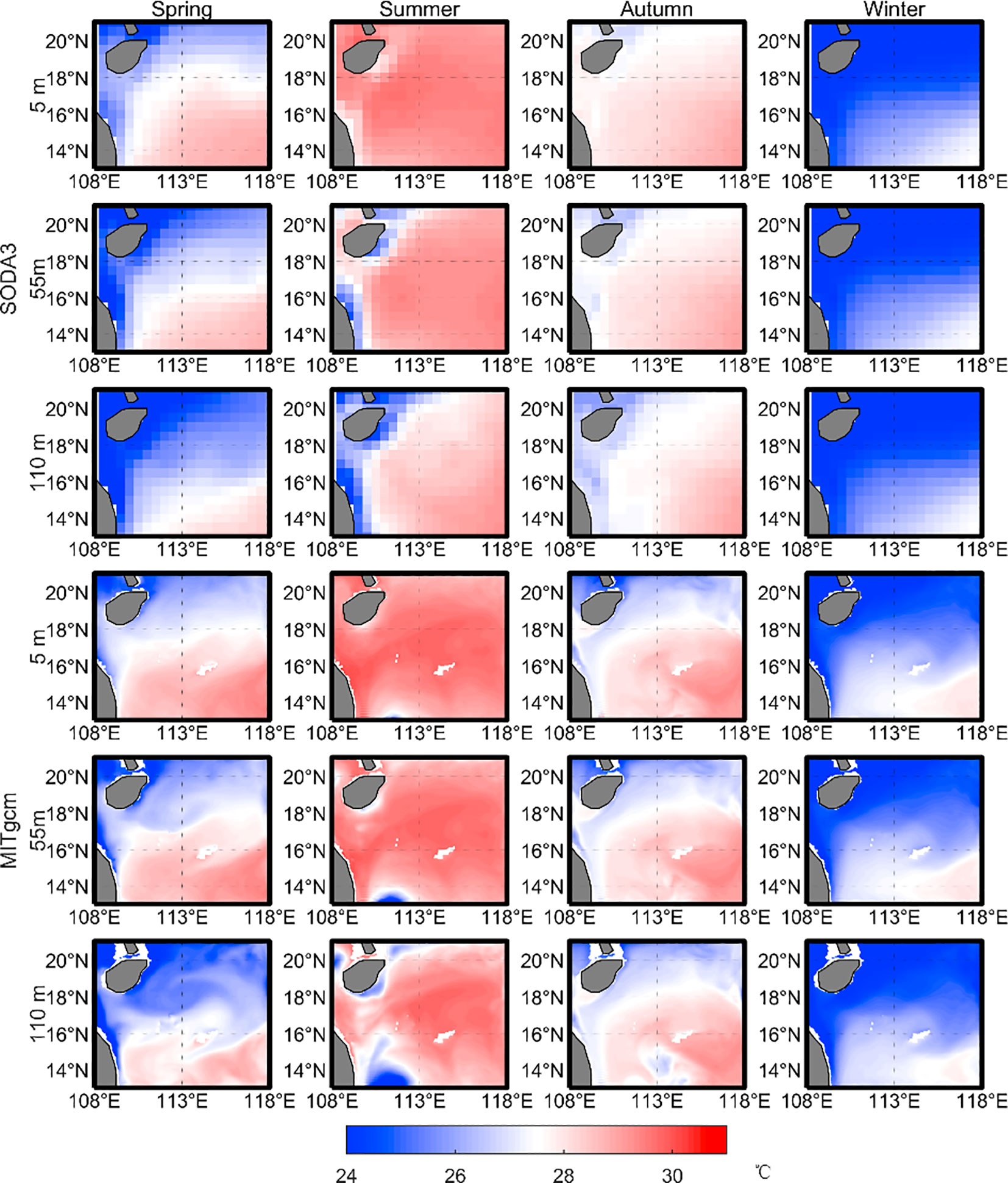
Figure 3 Seasonal variations of temperature. The first three rows are the SODA3 temperature at depths of 5 m (the first row), 55 m (the second row), and 110 m (the third row). The fourth–sixth rows are the MITgcm temperatures at depths of 5, 55, and 110 m, respectively.

FIGURE 4

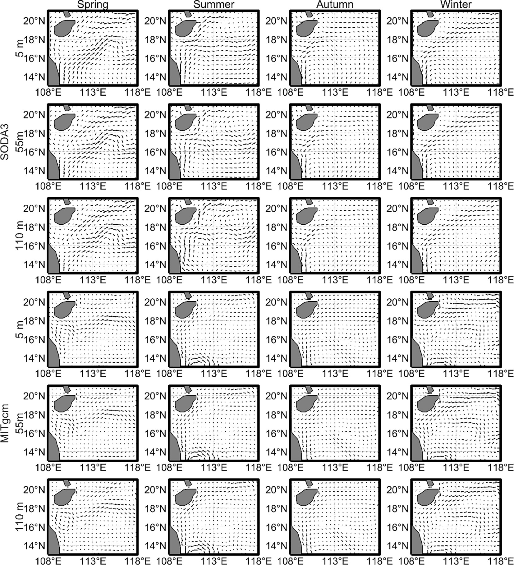
Figure 4 Seasonal variations of velocities. The first three rows are the SODA3 velocities at depths of 5 m (the first row), 55 m (the second row), and 110 m (the third row). The fourth–sixth rows are the MITgcm velocities at depths of 5, 55, and 110 m, respectively.

2.2 Methods

2.2.1 Spectrum analysis

The horizontal isotropic wavenumber spectrum is an effective means of estimating the spatial critical values of submesoscale and mesoscale processes (Cao et al., 2019) and is commonly used in the processing of model data (Rocha et al., 2016; Li et al., 2019). Under the assumption of horizontal motion uniformity and isotropy, within the wavenumber range dominated by quasi-geostrophic motion, the slope of the kinetic energy spectrum follows a $k^{-3}$ power law (Charney, 1971). In the submesoscale range, the slope of the kinetic energy spectrum is relatively flat and follows a $k^{-2}$ power law. Many observational and simulation results have confirmed this conclusion (Callies and Ferrari, 2013; Rocha et al., 2016; Qiu et al., 2017; Cao et al., 2019; Zhang et al., 2020a; Cao et al., 2023). This suggests that by determining the wavenumbers corresponding to the transition between $k^{-3}$ and $k^{-2}$ in the horizontal wavenumber spectrum, the spatial upper limit of submesoscale processes can be estimated.

The Python program provided by Rocha et al. (2016) is used to estimate and plot the horizontal isotropic wavenumber spectrum. The program first removes the linear trend of the raw data, then performs a two-dimensional discrete Fourier transform on the data and multiplies it by a two-dimensional Hanning window. Subsequently, the power spectral density of the meridional and zonal velocities is obtained separately through spectral estimation methods. Finally, the two-dimensional kinetic energy spectrum is synthesized based on the following formula,

$\begin{array}{ll}{\mathit{\text{spec}}}_{2\mathit{\text{D}}}=\frac{{\mathit{\text{spec}}}_{\mathit{\text{u}}}+{\mathit{\text{spec}}}_{\mathit{v}}}{2}& (1)\end{array}$

where ${\mathit{\text{spec}}}_{2\mathit{\text{D}}}$, ${\mathit{\text{spec}}}_{\mathit{u}}$ and ${\mathit{\text{spec}}}_{\mathit{v}}$ represent the two-dimensional power spectral density and the power spectral density of the meridional and zonal velocities, respectively.

This study area includes both shallow coastal waters and open deep waters, with large differences in topography and water depth. This leads to differences in the Rossby radius of deformation between the shelf and open sea areas, and a single spatial critical value cannot be used to extract submesoscale processes in both areas, which must be discussed separately. This study uses the location of the 210-m isobath as the boundary between the shelf and open water areas.

We estimate the horizontal isotropic wavenumber spectrum of the S1 region on 2 January 2020, and the B1 region on 5 February 2020 (Figures 5, 6). The slope of the kinetic energy spectrum in the shelf area is close to $k^{-3}$ in the mesoscale range but gradually flattens with decreasing wavelength in the range of wavelengths less than 14 km, exhibiting a $k^{-2}$ power law (Figure 6A), indicating that submesoscale motion is active in this wavelength range. The slope of the horizontal isotropic wavenumber spectrum in the open water area changes near a wavelength of 30 km and is close to $k^{-2}$ in the submesoscale range (<30 km) (Figure 6B). Therefore, this study selects 14 and 30 km as the spatial critical values for mesoscale and submesoscale processes in the shelf and open water areas, respectively.

FIGURE 5

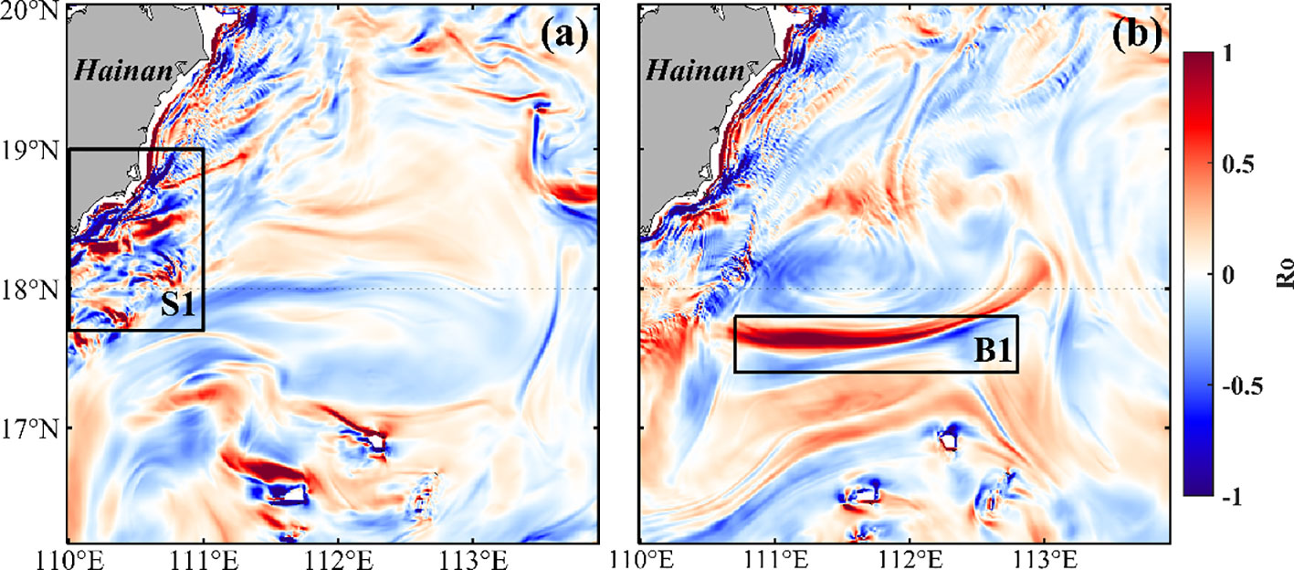
Figure 5 Distributions of Rossby number on (A) 2 January and (B) 5 February 2020.

FIGURE 6

Figure 6 Daily average wavenumber spectra for the 15- to 65-m layers in (A) the S1 region and (B) the B1 region.

Extracting submesoscale processes from full-spectrum data is a key step in submesoscale analysis (Wang et al., 2022). The Eulerian-based filtering method has been widely used for separating submesoscale processes, which includes temporal filtering (Barkan et al., 2017; Zhang et al., 2020a), spatial filtering (Dong et al., 2022; Song et al., 2022; Su et al., 2020b), and spatiotemporal filtering (Capet et al., 2008b; Qiu et al., 2018; Torres et al., 2018). In addition to the commonly used Eulerian filtering methods, many scholars have proposed different methods to improve the accuracy of submesoscale decomposition. For example, Wang et al. (2022) used the Lagrangian filtering method to remove the influence of mesoscale background flow, focusing only on the submesoscale VHT under the mesoscale eddy background. Wang et al. (2023a) proposed a dynamic decomposition method for ocean multiscale motion and successfully applied it to multiscale motion decomposition in the central SCS (Wang et al., 2023b).

This work employs a spatiotemporal filtering method to extract submesoscale processes. We adopt the Reynolds decomposition method to decompose the original physical quantities into annual average terms and perturbation terms. The perturbation terms are then decomposed into mesoscale and submesoscale components. The calculation formula is as follows:

$\begin{array}{ll}A=\overline{A}+(\tilde{A}-\overline{A})+(A-\tilde{A})=A_{\text{annual average}}+A_m+A_s& (2)\end{array}$

where $A$ denotes the physical quantity to be decomposed (such as $w$, $T$, $U$, $V$, etc.); $\overline{A}$ represents the annual mean result of the physical quantity; $A_m$ and $A_s$ represent the mesoscale and submesoscale components of the physical quantity, respectively; and $\tilde{A}$ is the spatiotemporal mean of the physical quantity $A$. In this study, 7 days are selected as the time-critical value for mesoscale and submesoscale processes (Torres et al., 2018; Wang et al., 2022), and 30 and 14 km are selected as the spatial critical values for open water and shelf area, respectively. $\tilde{A}$ is obtained by spatially averaging the physical quantity $A$ within a specified range (0.3° × 0.3° for open water, and 0.14° × 0.14° for shelf area) after 7-day averaging. As an example, the decomposition results of the vertical velocity $w$ at 12:00 on 1 January 2020 are shown in Figure 7.

FIGURE 7

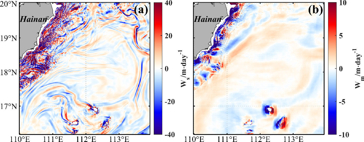
Figure 7 Decomposition results of the vertical velocity at 12:00 on 1 January 2020. (A, B) The distribution of submesoscale vertical velocity and mesoscale vertical velocity in the study area, respectively.

The submesoscale VHT is defined using the following formula:

$\begin{array}{ll}\text{VH}{T}_s=C_p\rho w_s{T}_s& (3)\end{array}$

where $C_p$ is the specific heat capacity of seawater, taken as 4,096 $\text{J}·{\text{kg}}^{-1}·°{\text{C}}^{-1}$; ρ is the density of seawater, taken as 1,024 $\text{kg}·{\text{m}}^{-3}$; and $w_s \text{and }{T}_s$ are the submesoscale components of vertical velocity and water temperature, respectively. Similarly, the mesoscale vertical heat transport can also be obtained from the following formula:

$\begin{array}{ll}\text{VH}{T}_m=C_p\rho w_m{T}_m& (4)\end{array}$

where $w_m$ and $T_m$ are the mesoscale components of vertical velocity and temperature, respectively.

3 Seasonal variations of VHT in shelf and open water

3.1 Seasonal variation in submesoscale motions

Figure 8 shows the spatial distribution of $\left|R_o\right|$ at 25-m depth on 10 January, 10 April, 10 July, and 10 October, respectively. The $\left|R_o\right|$ is larger in the Qiongdong shelf region and around Xisha Islands. The former is large in summer and weak in winter, which may be induced by summer coastal upwelling (Xie et al., 2012; Hu and Wang, 2016; Shi et al., 2021; Zhu et al., 2023). Figure 9 shows the seasonal variations of vertical velocity. Both the Rossby number, $\left|R_o\right|$, and vertical velocity achieve maximum values in winter (${\left|R_o\right|}_{\text{max}}=4.1$, $w_{\text{max}}=227$ m/day) in the open water, and 10.54% of this area has a vertical velocity of >10 m/day. The maximum vertical velocity is smaller than that revealed by Lin et al. (2020), who used MITgcm LLC4320 products. This difference may be induced by tidal effect: our model excludes tides but MITgcm LLC4320 includes tidal effect. The filament and eddy structures are more evident in the map of vertical velocity in terms of positive and negative values of filament. This may be induced by straining front, which enhances lateral buoyancy fluxes and the baroclinic instability, driving submesoscale processes and secondary current (Klein and Lapeyre, 2009; McWilliams, 2017; Pham and Sarkar, 2018; Zheng and Jing, 2022).

FIGURE 8

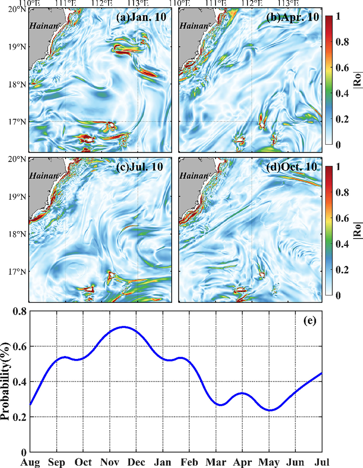
Figure 8 Seasonal variations in the absolute value of the Rossby number in the 25-m layer on 10 January, 2020 (A), 10 April 2020 (B), 10 July 2020 (C), and 10 October 2019 (D). (E) Monthly variation in Rossby number.

FIGURE 9

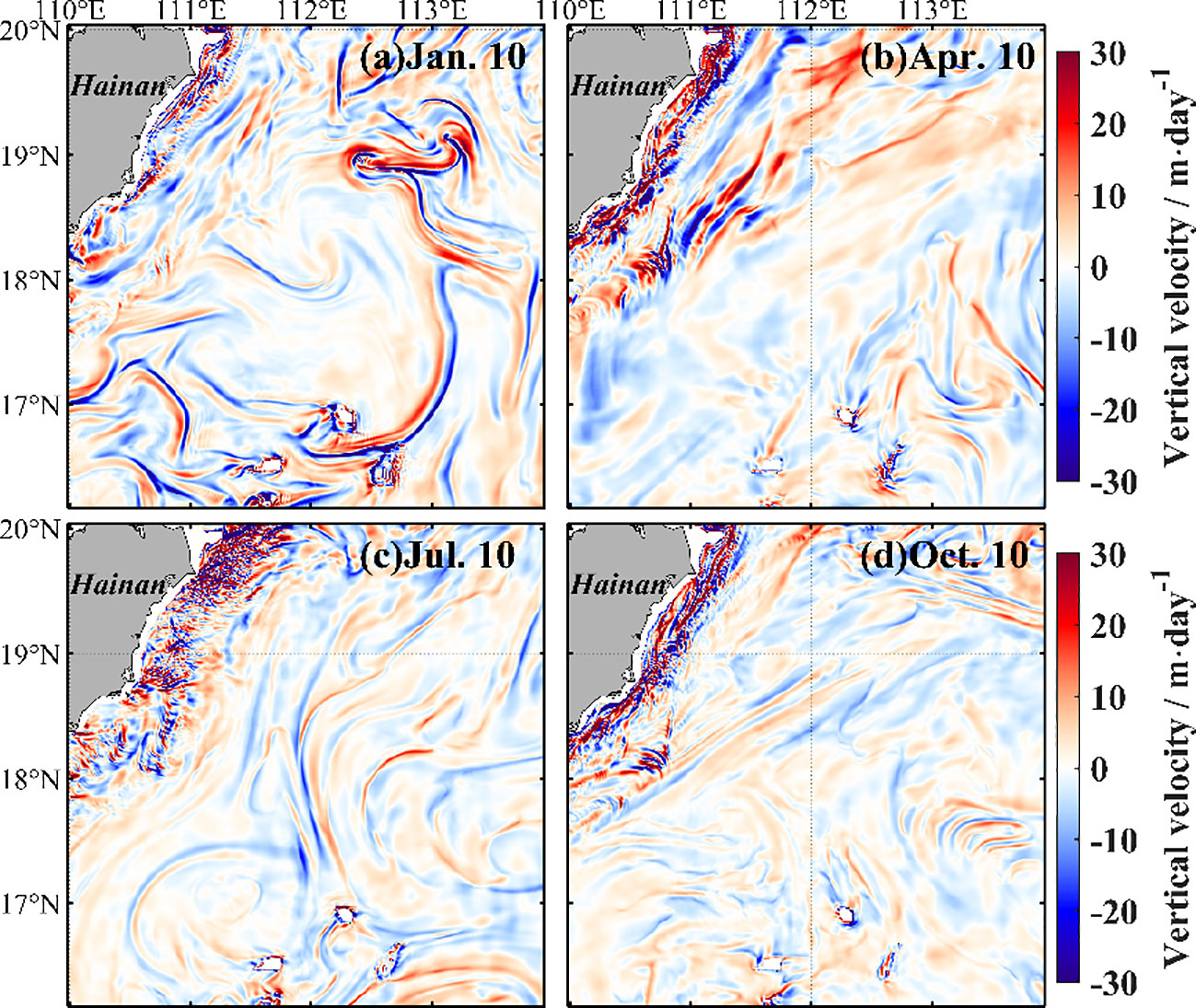
Figure 9 Spatial distribution of submesoscale vertical velocities in the 25-m layer on 10 January 2020 (A), 10 April 2020 (B), 10 July, 2020 (C), and 10 October 2019 (D).

3.2 Seasonal variation in submesoscale VHT

Figure 10 shows the seasonal variation of submesoscale VHT. In open water, the submesoscale VHT is strongest in winter, and the upward submesoscale VHT dominates the whole submesoscale VHT. That is, the submesoscale process transports heat from deeper, colder water to the surface’s warm layer. The maximum submesoscale VHT achieves 50.4 $\text{W}/{\text{m}}^2$, which is comparable to the results ($>40 \text{W}/m^2$) of Zhang et al. (2020b). Zhang et al. (2020a) suggested that mixed layer depth and mesoscale straining are important factors for the seasonal variation in the submesoscale process. The deeper mixed layer depth and stronger wind speed may induce mixed layer baroclinic instabilities (Zhang et al., 2020a; Tang et al., 2023) and thus trigger stronger VHT in the open sea in winter.

FIGURE 10

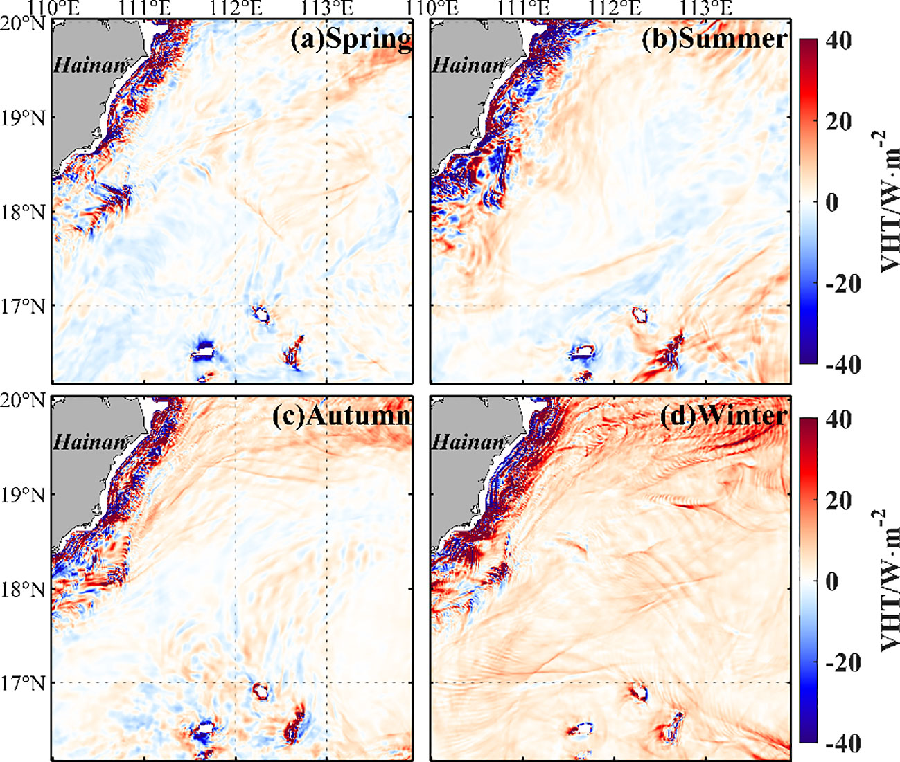
Figure 10 Spatial distribution of seasonally averaged submesoscale vertical heat transport in spring (A), summer (B), autumn (C), and winter (D).

In Hainan’s east shelf region, the submesoscale VHT is larger in winter and summer (Table 1). The maximum submesoscale VHT in this shelf region is >1,000 $\text{W}/{\text{m}}^2$ in all seasons, which is two orders larger than that in open water. This large VHT may be attributed to the coastal upwelling, downwelling, and associated coastal front (e.g., Jing et al., 2015). Also, secondary current along the coastal front was revealed by Xie et al. (2017), who suggested submesoscale processes appeared with alternating positive–negative vertical velocity alongshore bands by using a generalized omega equation. The area (VHT >20 $\text{W}/{\text{m}}^2$) occupies a greater probability than that in the open water. This means the submesoscale VHT contributions of coastal shelf region is non-negligible.

TABLE 1

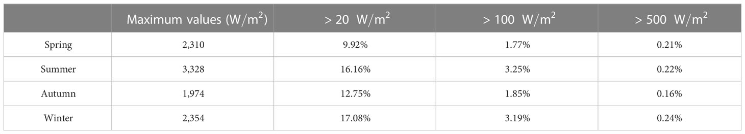
Table 1 Probability of absolute values of seasonally averaged submesoscale vertical heat transport greater than 20, 100, and 500 $\text{W}/{\text{m}}^2$ and maximum values of seasonally averaged submesoscale vertical heat transport in the shelf region.

The seasonal variations of regional mean submesoscale VHT in the shelf region and open water are also compared. The regional mean submesoscale VHT in the shelf region is about three times as large as that in the open water in winter. The submesoscale VHT in the shelf region takes up 45.91% of all the submesoscale VHT, although the area of the shelf region is only 26.1%. The annual mean values of submesoscale VHT in shelf region and open water is 4.1 and 2.4 $\text{W}/{\text{m}}^2$, respectively. These values are smaller than the global mean values of $9 \pm 3.5 \text{W}/{\text{m}}^2$ (Su et al., 2018).

3.3 The VHT difference between mesoscale and submesoscale processes

As mesoscale processes are popular in our study area. We compare the submesoscale VHT and mesoscale VHT in Figures 11 and 12. The absolute value of mesoscale VHT is larger than that of submesoscale VHT, especially in the shelf region. The net VHT from the mesoscale is negative in the shelf region, except in winter when downwelling dominates the coastal shelf region caused by northeasterly wind. For open water, the seasonal variation in mesoscale VHT is insignificant. The upward VHT induced by submesoscale processes takes up >80% of the area in winter and then around 50% in spring, while the VHT induced by mesoscale processes takes up 50% all around the year in shelf and open water.

FIGURE 11

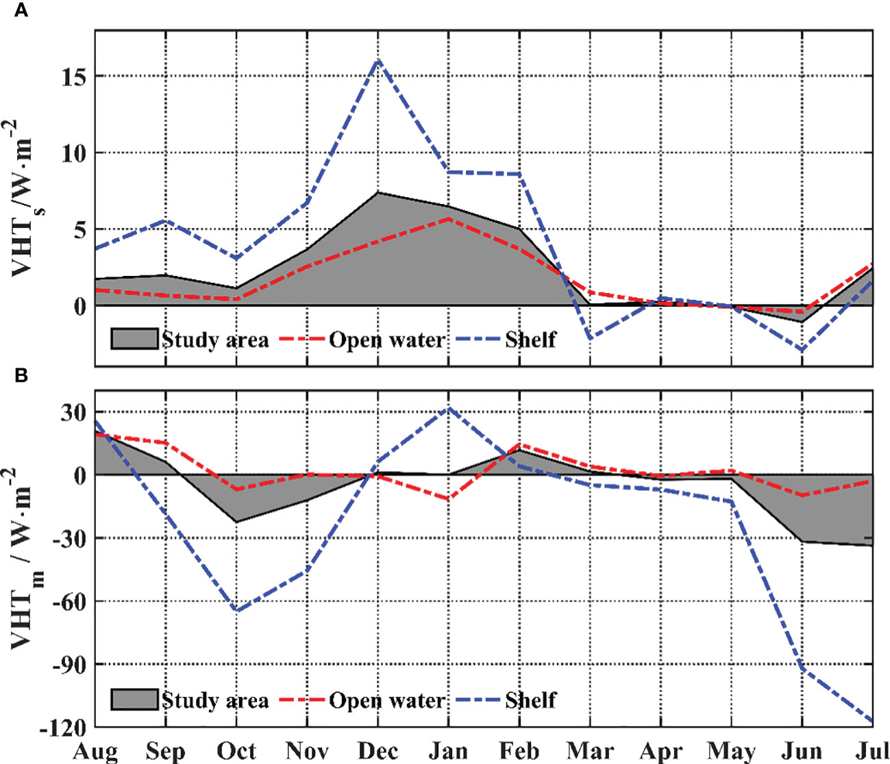
Figure 11 Time series of monthly averaged (A) submesoscale vertical heat transport and (B) mesoscale vertical heat transport in the 25-m layer. The red and blue lines are for the open water and shelf areas, respectively. The gray area is the result of averaging across the study area.

FIGURE 12

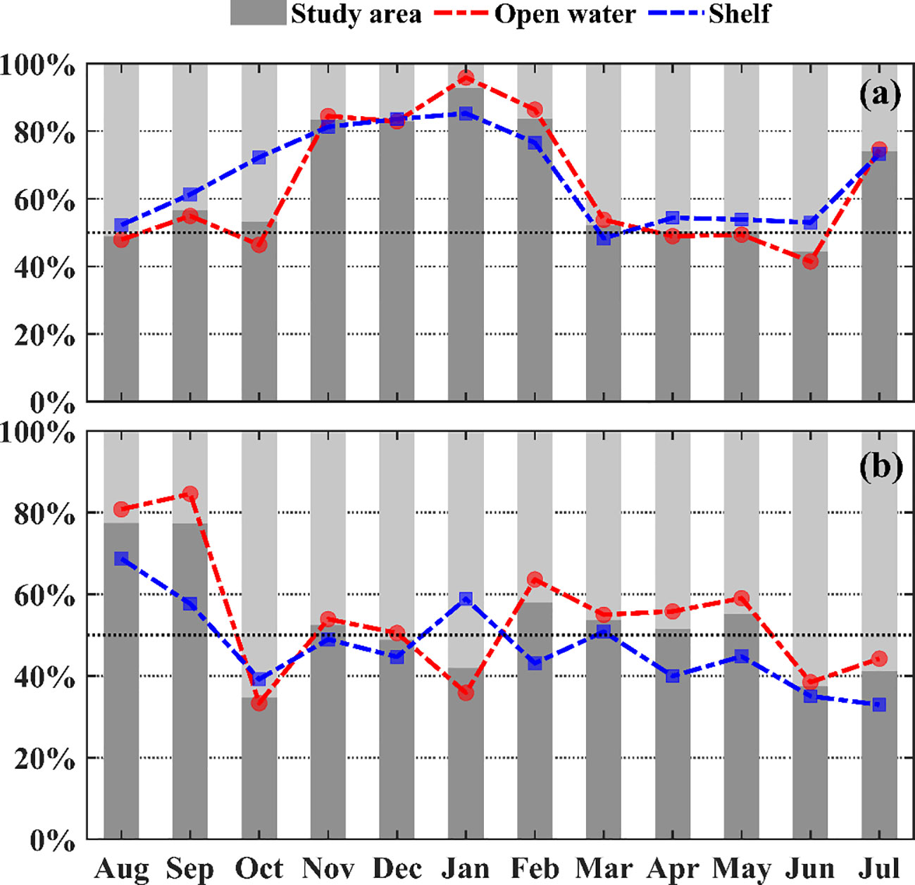
Figure 12 Area percentage of monthly averaged submesoscale upward heat transport in the 25 m layer. (A) Submesoscale vertical heat transport; (B) mesoscale vertical heat transport.

4 Intra-seasonal variation of submesoscale VHT

4.1 Disturbances of tropical cyclones

Time-serials of the probability with $\left|R_o\right|>1$ and submesoscale VHT, are shown in Figure 13. The VHT has an intra-seasonal variability signal, especially from autumn to winter. Notably, after a tropical cyclone (the gray shaded), the probability with $\left|R_o\right|>1$ increases sharply, and the peak value sustains around one week. The submesoscale VHT also appears large oscillation amplitude, and high-frequency oscillation of submesoscale VHT becomes significant after a tropical cyclone. The maximum amplitude of submesoscale VHT approaches 33.8 W/m² during “Podul” from August 29^th to 30^th, 2019.

FIGURE 13

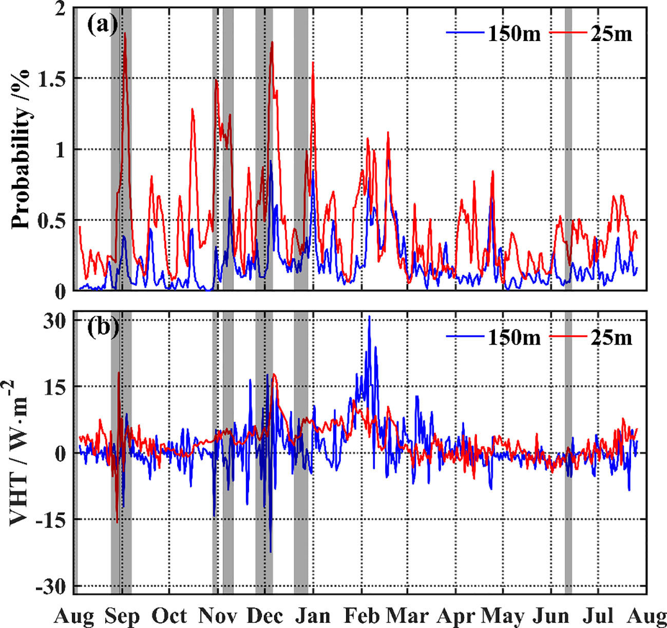
Figure 13 (A) Temporal variation of the probability that the absolute value of the daily averaged Rossby number is greater than 1. (B) Temporal variation of the daily averaged submesoscale vertical heat transport in the study area. The blue and red lines represent the 150- and 25-m layers, respectively. The gray area represents that the northern South China Sea was influenced by tropical cyclones during that time.

The tropical cyclone may change the current of mesoscale processes (Chen et al., 2013), injecting negative potential vorticity into the mesoscale eddies (Lu et al., 2016), and then may regulate the submesoscale motions through geostrophic straining or frontogenesis process. On the other hand, the interaction between inertial oscillation and submesoscale process may be exerted by tropical cyclones.

4.2 Disturbances of life stage of submesoscale eddies

Mesoscale geostrophic straining is a key factor for the generation of submesoscale motions (e.g., McWilliams, 2016; Zhang and Qiu, 2020). It has been suggested that the temporal variation of submesoscale motion within a mesoscale eddy is up to the geostrophic straining (Qiu et al., 2022a). The evolution of submesoscale eddies also attributes to the development of the VHT belt. We separate the life stage of a submesoscale eddy as birth, developing, mature, and cascade stages, referring to the definition of the atmospheric life-cycle stage. That is, the stage when the isolines of SLA are not closed but disturbed is taken as the birth stage; the stage when several closed SLA isolines come out is taken as the developing stage; the stage when the isolines of SLA achieve maximum is taken as mature stage; the stage after the mature stage is the cascade stage. This kind of separation for mesoscale eddies has been adopted by Yang et al. (2019).

Figure 14A shows a birth stage of a cold eddy on 7 December, when the streamlines are not closed. The sea level anomaly is 2 cm lower than the surrounding water. The maximum submesoscale VHT with a value of 209.0 $\text{W}/{\text{m}}^2$ locates at the edge of the cold eddy (Figure 14). On 10 December (Figure 14B), some developing eddies appear with closed SLA contours, and the maximum VHT belt also exists at the eddy edge but has an entrainment trend. Until 13 December (Figure 12C), most eddies are in the mature stage, and a well-spiral structure of high VHT belt appears within the mesoscale eddy. On 17 December (Figure 14D), the mesoscale eddy dissipates. The corresponding VHT becomes weak. It provides a good relationship between the VHT and the life stage of a submesoscale eddy.

FIGURE 14

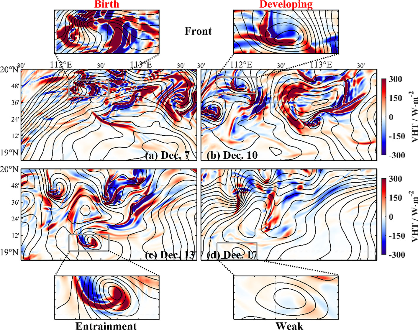
Figure 14 Relationship between eddy life stage and submesoscale VHT. Sea level anomaly (contour) and vertical heat transport (color) on 7 December (A, birth stage), December 10th (B, developing stage), 13 December (C, mature stage), and 17 December (D, cascade stage).

The submesoscale motions have strong vertical velocity, which induces significant vertical heat transport and may cause high surface chlorophyll-a concentrations. Figure 15 shows the chlorophyll-a distribution at different life stages of the eddy. At the birth stage (Figure 15A), the high chlorophyll-a concentration locates at an eddy center; at the developing stage (Figure 15B), the maximum chlorophyll-a concentration has an entrainment trend, which looks like the maximum VHT belt; at the mature stage (Figure 15C), the spiral structure of chlorophyll-a concentration is more significant, although the value of chlorophyll-a concentration becomes lower than at developing stage; at cascade stage(Figure 15D), chlorophyll-a concentration becomes quite low.

FIGURE 15

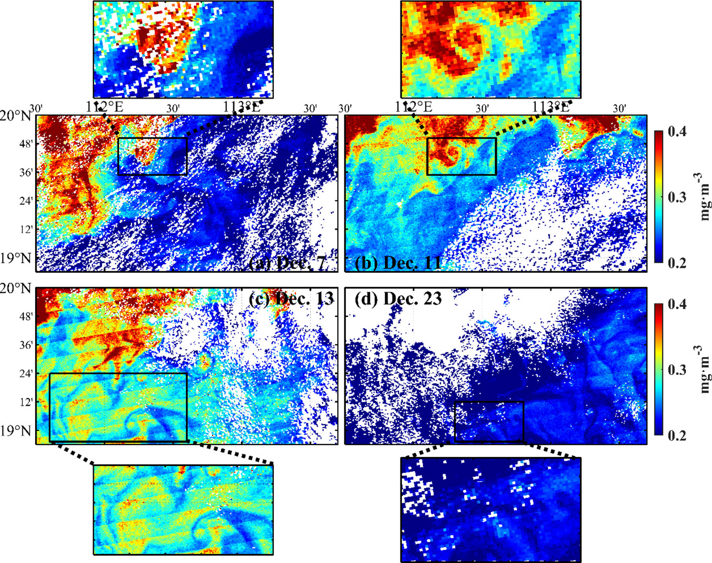
Figure 15 Relationship between eddy life stage and chlorophyll-a concentration on 7 December (A, birth stage), 11 December (B, developing stage), 13 December (C, mature stage), and 23 December (D, cascade stage). The black boxes indicate the corresponding life stage of the eddy.

The submesoscale motions may result from mesoscale geostrophic straining. Zhang and Qiu (2020) suggested the spiral structures of the chlorophyll-a belt are caused by mesoscale geostrophic straining, which is related to the life stage of mesoscale eddy. Here, we found the life stage of submesoscale eddy plays the same roles in the structure of chlorophyll-a and VHT. It indicates that, besides frontogenesis and mesoscale geostrophic straining, submesoscale velocity straining may be another possible mechanism for submesoscale motions. Our numerical model has successfully provided the life stage and the associated VHT of submesoscale eddies.

5 Summary

Submesoscale motions with large vertical velocities could induce strong vertical heat and matter transport. Here, the vertical heat transport induced by submesoscale motions has been estimated by using a 1-km high-resolution MITgcm. The VHT has different seasonal variations in the shelf sea and open sea regions: in the shelf region, the VHT is strong in summer, which may be induced by summer upwelling; in the open sea, the VHT is strong in winter and weak in summer. The submesoscale VHT in the shelf region accounts for 46% of the total submesoscale VHT in the region, indicating an important role in the regional ocean current. Both the tropical cyclone and life stage of submesoscale eddies influence the activity and VHT of submesoscale. Tropical cyclones usually enhance the submesoscale VHT. The VHT is strongest at the birth stage of the submesoscale eddy, and so is the surface chlorophyll-a concentration. The dynamics of the strong submesoscale VHT induced by tropical cyclones and submesoscale eddies need further study.

Data availability statement

The raw data supporting the conclusions of this article will be made available by the authors, without undue reservation.

Author contributions

All authors contributed to the study conception and design. Material preparation, data collection and analysis were performed by HP, CQ, and HL. The first draft of the manuscript was written by CQ and all authors commented on previous versions of the manuscript. All authors read and approved the final manuscript.

Funding

This study was supported by the National Natural Science Foundation of China (Grant No. 42227901 and No. 41976002) and the Project of the Southern Marine Science and Engineering Guangdong Laboratory (Zhuhai) (Grant No. SML2021SP205).

Conflict of interest

The authors declare that the research was conducted in the absence of any commercial or financial relationships that could be construed as a potential conflict of interest.

Publisher’s note

All claims expressed in this article are solely those of the authors and do not necessarily represent those of their affiliated organizations, or those of the publisher, the editors and the reviewers. Any product that may be evaluated in this article, or claim that may be made by its manufacturer, is not guaranteed or endorsed by the publisher.

References

Bachman S. D., Taylor J. R., Adams K. A., Hosegood P. J. (2017). Mesoscale and Submesoscale effects on mixed layer depth in the Southern Ocean. J. Phys. Oceanogr. 47, 2173–2188. doi: 10.1175/JPO-D-17-0034.1

CrossRef Full Text | Google Scholar

Barkan R., Winters K. B., McWilliams J. C. (2017). Stimulated imbalance and the enhancement of Eddy Kinetic Energy dissipation by internal waves. J. Phys. Oceanogr. 47, 181–198. doi: 10.1175/JPO-D-16-0117.1

CrossRef Full Text | Google Scholar

Brannigan L. (2016). Intense submesoscale upwelling in anticyclonic eddies. Geophys. Res. Lett. 43, 3360–3369. doi: 10.1002/2016GL067926

CrossRef Full Text | Google Scholar

Callies J., Ferrari R. (2013). Interpreting energy and tracer Spectra of Upper-Ocean Turbulence in the Submesoscale range (1–200 km). J. Phys. Oceanogr. 43, 2456–2474. doi: 10.1175/JPO-D-13-063.1

CrossRef Full Text | Google Scholar

Cao H., Fox-Kemper B., Jing Z., Song X., Liu Y. (2023). Towards the Upper-Ocean unbalanced Submesoscale motions in the Oleander observations. J. Phys. Oceanogr 53 (4), 1123–1138. doi: 10.1175/JPO-D-22-0134.1

CrossRef Full Text | Google Scholar

Cao H., Jing Z. (2022). Submesoscale Ageostrophic motions within and below the mixed layer of the Northwestern Pacific Ocean. J. Geophys. Res. Oceans 127, e2021JC017812. doi: 10.1029/2021JC017812

CrossRef Full Text | Google Scholar

Cao H., Jing Z., Fox-Kemper B., Yan T., Qi Y. (2019). Scale transition from Geostrophic motions to internal waves in the Northern South China Sea. J. Geophys. Res. Oceans 124, 9364–9383. doi: 10.1029/2019JC015575

CrossRef Full Text | Google Scholar

Cao H., Meng X., Jing Z., Yang X. (2022). High-resolution simulation of upper-ocean submesoscale variability in the South China Sea: Spatial and seasonal dynamical regimes. Acta Oceanol. Sin. 41, 26–41. doi: 10.1007/s13131-022-2014-4

CrossRef Full Text | Google Scholar

Capet X., McWilliams J. C., Molemaker M. J., Shchepetkin A. F. (2008a). Mesoscale to Submesoscale transition in the California current system. Part II: Frontal processes. J. Phys. Oceanogr. 38, 44–64. doi: 10.1175/2007JPO3672.1

CrossRef Full Text | Google Scholar

Capet X., McWilliams J. C., Molemaker M. J., Shchepetkin A. F. (2008b). Mesoscale to Submesoscale transition in the California current system. Part I: Flow structure, Eddy Flux, and observational tests. J. Phys. Oceanogr. 38, 29–43. doi: 10.1175/2007JPO3671.1

CrossRef Full Text | Google Scholar

Charney J. G. (1971). Geostrophic Turbulence. J. Atmospheric Sci. 28, 1087–1095. doi: 10.1175/1520-0469(1971)028<1087:GT>2.0.CO;2

CrossRef Full Text | Google Scholar

Chen J., Hu Z. (2023). Seasonal variability in spatial patterns of sea surface cold- and warm fronts over the continental shelf of the northern South China Sea. Front. Mar. Sci. 9. doi: 10.3389/fmars.2022.1100772

CrossRef Full Text | Google Scholar

Chen D., Lei X., Wang W., Wang G., Han G., Zhou L. (2013). Upper ocean response and feedback mechanisms to Typhoon. Adv. Earth Sci. Chin. 28, 1077–1086. doi: 10.11867/j.issn.1001-8166.2013.10.1077

CrossRef Full Text | Google Scholar

Dong J., Fox-Kemper B., Zhang H., Dong C. (2021). The scale and activity of symmetric instability estimated from a global submesoscale-permitting ocean model. J. Phys. Oceanogr. 51, 1655–1670. doi: 10.1175/JPO-D-20-0159.1

CrossRef Full Text | Google Scholar

Dong J., Jing Z., Fox-Kemper B., Wang Y., Cao H., Dong C. (2022). Effects of symmetric instability in the Kuroshio Extension region in winter. Deep Sea Res. Part II Top. Stud. Oceanogr. 202, 105142. doi: 10.1016/j.dsr2.2022.105142

CrossRef Full Text | Google Scholar

Dong J., Zhong Y. (2018). The spatiotemporal features of submesoscale processes in the northeastern South China Sea. Acta Oceanol. Sin. 37, 8–18. doi: 10.1007/s13131-018-1277-2

CrossRef Full Text | Google Scholar

Dong J., Zhong Y. (2020). Submesoscale fronts observed by satellites over the Northern South China Sea shelf. Dyn. Atmospheres Oceans 91, 101161. doi: 10.1016/j.dynatmoce.2020.101161

CrossRef Full Text | Google Scholar

Hu J., Wang X. H. (2016). Progress on upwelling studies in the China seas. Rev. Geophys. 54, 653–673. doi: 10.1002/2015RG000505

CrossRef Full Text | Google Scholar

Jiang Y., Dong J., Zhang X., Zhang W., Wang H., Zhang W. (2022). Evaluating the effects of a symmetric instability parameterization scheme in the Xisha-Zhongsha waters, South China Sea in winter. Front. Mar. Sci. 9. doi: 10.3389/fmars.2022.985605

PubMed Abstract | CrossRef Full Text | Google Scholar

Jiang Y., Zhang W., Wang H., Zhang X. (2023). Assessing the Spatio-Temporal features and mechanisms of symmetric instability activity probability in the central part of the South China Sea based on a Regional ocean model. J. Mar. Sci. Eng. 11, 431. doi: 10.3390/jmse11020431

CrossRef Full Text | Google Scholar

Jing Z. Y., Fox-Kemper B., Cao H., Zheng R., Du Y. (2020). Submesoscale fronts and their dynamical processes associated with symmetric instability in the Northwest Pacific Subtropical Ocean. J. Phys. Oceanogr. 51, 83–100. doi: 10.1175/JPO-D-20-0076.1

CrossRef Full Text | Google Scholar

Jing Z., Qi Y., Du Y., Zhang S., Xie L. (2015). Summer upwelling and thermal fronts in the northwestern South China Sea: Observational analysis of two mesoscale mapping surveys. J. Geophys. Res. Oceans 120, 1993–2006. doi: 10.1002/2014JC010601

CrossRef Full Text | Google Scholar

Klein P., Lapeyre G. (2009). The oceanic vertical pump induced by Mesoscale and Submesoscale turbulence. Annu. Rev. Mar. Sci. 1, 351–375. doi: 10.1146/annurev.marine.010908.163704

CrossRef Full Text | Google Scholar

Large W. G., McWilliams J. C., Doney S. C. (1994). Oceanic vertical mixing: A review and a model with a nonlocal boundary layer parameterization. Rev. Geophysics 32 (4), 363–403. doi: 10.1029/94RG01872

CrossRef Full Text | Google Scholar

Large W. G., Yeager S. G. (2009). The global climatology of an interannually varying air–sea flux data set. Clim. Dyn. 33, 341–364. doi: 10.1007/s00382-008-0441-3

CrossRef Full Text | Google Scholar

Li J., Dong J., Yang Q., Zhang X. (2019). Spatial-temporal variability of submesoscale currents in the South China Sea. J. Oceanol. Limnol. 37, 474–485. doi: 10.1007/s00343-019-8077-1

CrossRef Full Text | Google Scholar

Lin H., Liu Z., Hu J., Menemenlis D., Huang Y. (2020). Characterizing meso- to submesoscale features in the South China Sea. Prog. Oceanogr. 188, 102420. doi: 10.1016/j.pocean.2020.102420

CrossRef Full Text | Google Scholar

Liu Z., He C., Lu F. (2018). Local and remote responses of atmospheric and oceanic heat transports to climate forcing: compensation versus collaboration. J. Clim. 31, 6445–6460. doi: 10.1175/JCLI-D-17-0675.1

CrossRef Full Text | Google Scholar

Liu G., He Y., Shen H., Qiu Z. (2010). Submesoscale activity over the shelf of the northern South China Sea in summer: simulation with an embedded model. Chin. J. Oceanol. Limnol. 28, 1073–1079. doi: 10.1007/s00343-010-0030-2

CrossRef Full Text | Google Scholar

Lu Z., Wang G., Shang X. (2016). Response of a preexisting cyclonic ocean Eddy to a Typhoon. J. Phys. Oceanogr 46 (8), 2403~2410. doi: 10.1175/JPO-D-16-0040.1

CrossRef Full Text | Google Scholar

Martin M., Dash P., Ignatov A., Banzon V., Beggs H., Brasnett B., et al. (2012). Group for High Resolution sea Surface temperature (GHRSST) analysis fields inter-comparisons. Part 1: a GHRSST multi-product ensemble (GMPE). Deep-Sea Res. II Top. Stud. Oceanogr 77–80, 21–30. doi: 10.1016/j.dsr2.2012.04.013

CrossRef Full Text | Google Scholar

McWilliams J. C. (2016). Submesoscale currents in the ocean. Proc. R. Soc Math. Phys. Eng. Sci. 472, 20160117. doi: 10.1098/rspa.2016.0117

CrossRef Full Text | Google Scholar

McWilliams J. C. (2017). Submesoscale surface fronts and filaments: secondary circulation, buoyancy flux, and frontogenesis. J. Fluid Mech. 823, 391–432. doi: 10.1017/jfm.2017.294

CrossRef Full Text | Google Scholar

Nummelin A., Li C., Hezel P. J. (2017). Connecting ocean heat transport changes from the midlatitudes to the Arctic Ocean. Geophys. Res. Lett. 44, 1899–1908. doi: 10.1002/2016GL071333

CrossRef Full Text | Google Scholar

Omand M. M., D’Asaro E. A., Lee C. M., Perry M. J., Briggs N., Cetinić I., et al. (2015). Eddy-driven subduction exports particulate organic carbon from the spring bloom. Science 348, 222–225. doi: 10.1126/science.1260062

PubMed Abstract | CrossRef Full Text | Google Scholar

Pham H. T., Sarkar S. (2018). Ageostrophic secondary circulation at a Submesoscale front and the formation of gravity currents. J. Phys. Oceanogr. 48, 2507–2529. doi: 10.1175/JPO-D-17-0271.1

CrossRef Full Text | Google Scholar

Qiu B., Chen S., Klein P., Sasaki H., Sasai Y. (2014). Seasonal Mesoscale and Submesoscale Eddy variability along the North Pacific Subtropical countercurrent. J. Phys. Oceanogr. 44, 3079–3098. doi: 10.1175/JPO-D-14-0071.1

CrossRef Full Text | Google Scholar

Qiu B., Chen S., Klein P., Wang J., Torres H., Fu L.-L., et al. (2018). Seasonality in transition scale from balanced to unbalanced motions in the world ocean. J. Phys. Oceanogr. 48, 591–605. doi: 10.1175/JPO-D-17-0169.1

CrossRef Full Text | Google Scholar

Qiu C., Mao H., Liu H., Xie Q., Yu J., Su D., et al. (2019). Deformation of a warm Eddy in the Northern South China Sea. J. Geophys. Res. Oceans 124, 5551–5564. doi: 10.1029/2019JC015288

CrossRef Full Text | Google Scholar

Qiu B., Nakano T., Chen S., Klein P. (2017). Submesoscale transition from geostrophic flows to internal waves in the northwestern Pacific upper ocean. Nat. Commun. 8, 14055. doi: 10.1038/ncomms14055

PubMed Abstract | CrossRef Full Text | Google Scholar

Qiu C., Yang Z., Wang D., Feng M., Su J. (2022a). The enhancement of Submesoscale Ageostrophic motion on the mesoscale Eddies in the South China Sea. J. Geophys. Res. Oceans 127, e2022JC018736. doi: 10.1029/2022JC018736

CrossRef Full Text | Google Scholar

Qiu C., Yi Z., Su D., Wu Z., Liu H., Lin P., et al. (2022b). Cross-slope heat and salt transport induced by slope intrusion Eddy’s horizontal asymmetry in the Northern South China Sea. J. Geophys. Res. Oceans 127, e2022JC018406. doi: 10.1029/2022JC018406

CrossRef Full Text | Google Scholar

Rocha C. B., Chereskin T. K., Gille S. T., Menemenlis D. (2016). Mesoscale to Submesoscale wavenumber spectra in Drake Passage. J. Phys. Oceanogr. 46, 601–620. doi: 10.1175/JPO-D-15-0087.1

CrossRef Full Text | Google Scholar

Shi W., Huang Z., Hu J. (2021). Using TPI to map spatial and temporal variations of significant coastal upwelling in the Northern South China Sea. Remote Sens. 13, 1065. doi: 10.3390/rs13061065

CrossRef Full Text | Google Scholar

Shu Y., Wang Q., Zu T. (2018). Progress on shelf and slope circulation in the northern South China Sea. Sci. China Earth Sci. 61, 560–571. doi: 10.1007/s11430-017-9152-y

CrossRef Full Text | Google Scholar

Siegelman L. (2020). Energetic Submesoscale dynamics in the ocean interior. J. Phys. Oceanogr. 50, 727–749. doi: 10.1175/JPO-D-19-0253.1

CrossRef Full Text | Google Scholar

Siegelman L., Klein P., Rivière P., Thompson A. F., Torres H. S., Flexas M., et al. (2020). Enhanced upward heat transport at deep submesoscale ocean fronts. Nat. Geosci. 13, 50–55. doi: 10.1038/s41561-019-0489-1

CrossRef Full Text | Google Scholar

Song X., Xie X., Qiu B., Cao H., Xie S.-P., Chen Z., et al. (2022). Air-sea latent heat flux anomalies induced by oceanic Submesoscale processes: An Observational case study. Front. Mar. Sci. 9. doi: 10.3389/fmars.2022.850207

PubMed Abstract | CrossRef Full Text | Google Scholar

Su D., Lin P., Mao H., Wu J., Liu H., Cui Y., et al. (2020a). Features of slope intrusion Mesoscale Eddies in the Northern South China Sea. J. Geophys. Res. Oceans 125, e2019JC015349. doi: 10.1029/2019JC015349

CrossRef Full Text | Google Scholar

Su Z., Torres H., Klein P., Thompson A. F., Siegelman L., Wang J., et al. (2020b). High-frequency Submesoscale motions enhance the upward vertical heat transport in the global ocean. J. Geophys. Res. Oceans 125, e2020JC016544. doi: 10.1029/2020JC016544

CrossRef Full Text | Google Scholar

Su Z., Wang J., Klein P., Thompson A. F., Menemenlis D. (2018). Ocean submesoscales as a key component of the global heat budget. Nat. Commun. 9, 775. doi: 10.1038/s41467-018-02983-w

PubMed Abstract | CrossRef Full Text | Google Scholar

Tang H., Shu Y., Wang D., Xie Q., Zhang Z., Li J., et al. (2023). Submesoscale processes observed by high-frequency float in the western South China sea. Deep Sea Res. Part Oceanogr. Res. Pap. 192, 103896. doi: 10.1016/j.dsr.2022.103896

CrossRef Full Text | Google Scholar

Torres H. S., Klein P., Menemenlis D., Qiu B., Su Z., Wang J., et al. (2018). Partitioning ocean motions into balanced motions and internal gravity waves: A modeling study in anticipation of future space missions. J. Geophys. Res. Oceans 123, 8084–8105. doi: 10.1029/2018JC014438

CrossRef Full Text | Google Scholar

Wang Q., Dong C., Dong J., Zhang H., Yang J. (2022). Submesoscale processes-induced vertical heat transport modulated by oceanic mesoscale eddies. Deep Sea Res. Part II Top. Stud. Oceanogr. 202, 105138. doi: 10.1016/j.dsr2.2022.105138

CrossRef Full Text | Google Scholar

Wang C., Liu Z., Lin H. (2023a). On dynamical decomposition of multiscale oceanic motions. J. Adv. Model. Earth Syst. 15, e2022MS003556. doi: 10.1029/2022MS003556

CrossRef Full Text | Google Scholar

Wang C., Liu Z., Lin H. (2023b). A simple approach for disentangling vortical and wavy motions of oceanic flows. J. Phys. Oceanogr. 53 (5), 1237–1249. doi: 10.1175/JPO-D-22-0148.1

CrossRef Full Text | Google Scholar

Xie L., Enric P.-S., Zheng Q., Zhang S., Zong X., Yi X., et al. (2017). Diagnosis of 3-D vertical circulation in the upwelling and frontal zones east of Hainan Island, China. J. Phys. Oceanogr 47 (4), 755–774. doi: 10.1175/JPO-D-16-0192.1

CrossRef Full Text | Google Scholar

Xie L., Zhang S., Zhao H. (2012). Overview of studies on Qiongdong upwelling. J. Trop. Oceanogr. Chin. 31, 35–41. doi: 10.3969/j.issn.1009-5470.2012.04.007

CrossRef Full Text | Google Scholar

Yang H., Qiu B., Chang P., Wu L., Wang S., Chen Z., et al. (2018). Decadal variability of Eddy characteristics and energetics in the Kuroshio Extension: Unstable versus stable states. J. Geophys. Res. Oceans 123, 6653–6669. doi: 10.1029/2018JC014081

CrossRef Full Text | Google Scholar

Yang S., Song H., Coakley B., Zhang K., Fan W. (2022). A Mesoscale Eddy with Submesoscale spiral bands observed from seismic reflection sections in the Northwind Basin, Arctic Ocean. J. Geophys. Res. Oceans 127, e2021JC017984. doi: 10.1029/2021JC017984

CrossRef Full Text | Google Scholar

Yang Z., Wang G., Chen C. (2019). Horizontal velocity structure of mesoscale eddies in the South China Sea. Deep Sea Res. Part I: Oceanographic Res. Papers 149, 103055. doi: 10.1016/j.dsr.2019.06.001

CrossRef Full Text | Google Scholar

Yoo J. G., Kim S. Y., Kim H. S. (2018). Spectral descriptions of Submesoscale surface circulation in a Coastal Region. J. Geophys. Res. Oceans 123, 4224–4249. doi: 10.1029/2016JC012517

CrossRef Full Text | Google Scholar

Yu X., Garabato A. C. N., Martin A. P., Buckingham C. E., Brannigan L., Su Z. (2019). An annual cycle of Submesoscale vertical flow and restratification in the upper ocean. J. Phys. Oceanogr. 49, 1439–1461. doi: 10.1175/JPO-D-18-0253.1

CrossRef Full Text | Google Scholar

Zhang Z., Qiu B. (2020). Surface chlorophyll enhancement in Mesoscale Eddies by Submesoscale spiral bands. Geophys. Res. Lett. 47, e2020GL088820. doi: 10.1029/2020GL088820

CrossRef Full Text | Google Scholar

Zhang Z., Zhang Y., Qiu B., Sasaki H., Sun Z., Zhang X., et al. (2020a). Spatiotemporal characteristics and generation mechanisms of Submesoscale currents in the Northeastern South China Sea revealed by numerical simulations. J. Geophys. Res. Oceans 125, e2019JC015404. doi: 10.1029/2019JC015404

CrossRef Full Text | Google Scholar

Zhang Y., Zhang X., Zhang J., Sun Z., Zhang Z. (2020b). Spatiotemporal characteristics and vertical heat transport of Submesoscale processes in the South China Sea. Period. Ocean Univ. China (in Chinese) 50, 1–11. doi: 10.16441/j.cnki.hdxb.20200035

CrossRef Full Text | Google Scholar

Zheng R., Jing Z. (2022). Submesoscale-enhanced filaments and frontogenetic mechanism within mesoscale eddies of the South China Sea. Acta Oceanol. Sin. 41, 42–53. doi: 10.1007/s13131-021-1971-3

CrossRef Full Text | Google Scholar

Zheng Q., Xie L., Xiong X., Hu X., Chen L. (2020). Progress in research of submesoscale processes in the South China Sea. Acta Oceanol. Sin. 39, 1–13. doi: 10.1007/s13131-019-1521-4

CrossRef Full Text | Google Scholar

Zhong Y., Bracco A., Tian J., Dong J., Zhao W., Zhang Z. (2017). Observed and simulated submesoscale vertical pump of an anticyclonic eddy in the South China Sea. Sci. Rep. 7, 1–13. doi: 10.1038/srep44011

PubMed Abstract | CrossRef Full Text | Google Scholar

Zhu J., Zhou Q., Zhou Q., Geng X., Shi J., Guo X., et al. (2023). Interannual variation of coastal upwelling around Hainan Island. Front. Mar. Sci. 10. doi: 10.3389/fmars.2023.1054669

CrossRef Full Text | Google Scholar