High-resolution study of the air-sea CO2 flux and net community oxygen production in the Ligurian Sea by a fleet of gliders

Intense glider monitoring was conducted in the Ligurian Sea for five months to capture the Net Community Production (NCP) variability in one of the most dynamic and productive regions of the Mediterranean Sea. Using the SeaExplorer glider technology, we were able to observe continuously from January to the end of May 2018 the physical and biogeochemical variables during the last period of intense convection observed in this region. High-frequency measurements from these gliders provided valuable information for determining dissolved O₂ (DO) concentrations between coastal and open sea waters. Our DO balance approach provided an estimate of NCP fluxes complemented by the prediction of air-sea CO₂ fluxes based on a neural network adapted to the Mediterranean Sea (CANYON-MED). Based on our NCP calculation method, our results show that the air-sea O₂ flux and DO inventory have contributed largely to the NCP variability. The NCP values also suggest that heterotrophic conditions were predominant in winter and became autotrophic in spring, with strong variability in coastal waters due to the occurrence of sub-mesoscale structures. Finally, CO₂ fluxes at the air-sea interface reveal that during the convection period, the central zone of the Ligurian Sea acted as a CO₂ sink from January to March with little impact on NCP fluxes counterbalanced by a thermal effect of seawater.

1 Introduction

The ocean plays a critical role in the global carbon cycle, storing 50 times more carbon than the atmosphere and absorbing a quarter of global anthropogenic carbon emissions (Gruber et al., 2019). This absorption of CO₂ by seawater induces a decrease in pH which has an impact on chemical and biological processes (Doney et al., 2009). Deep convection zones are considered a more important sink for atmospheric CO₂, inducing significant CO₂ sequestration at the surface and transferred to the deep ocean by vertical mixing and biological pumping (Körtzinger et al., 2008). In the context of global warming and the reduction in the intensity of deep convection (Somot et al., 2016), their role as CO₂ sinks could be compromised in the future and thus worsen CO₂ emissions in general, although the fate of the mechanisms interacting in the carbon biological pump is still unclear (Bopp et al., 2013; Boyd et al., 2019).

The Mediterranean Sea is considered as a miniature ocean, where global-scale processes occur on smaller spatial and temporal scales than in other oceans (Álvarez et al., 2014). This marginal sea comprises just 0.8% of the global oceanic surface, but for its size is regarded as an important sink for anthropogenic carbon due to its physical and biogeochemical characteristics (Álvarez et al., 2014). The northwestern region is the most dynamic area of the Mediterranean Sea where winter deep convection occurs (Mertens and Schott, 1998; Bethoux et al., 2002). Due to the cyclonic circulation, the increase in density induced in the surface waters in winter by cold and dry northerly winds produces instabilities in the water column leading to vertical mixing of the surface waters with deeper waters. This process occurs mainly in the Gulf of Lion and the Ligurian Sea when the convection is intense with strong inter-annual variability (Estournel et al., 2016; Houpert et al., 2016; Testor et al., 2018). In the Ligurian Sea, the observations conducted since the 1990s show a clear increase in temperature and salinity (Bethoux et al., 2002; Marty and Chiavérini, 2010) followed by an increase of pCO₂ and associated with a decrease of pH over the last 18 years from the surface to deep waters (Merlivat et al., 2018; Coppola et al., 2020).

In the context of the carbon cycle, CO₂ exchange at the air-sea interface (F_CO2) represents the amount of atmospheric CO₂ captured at the ocean surface, some of which will be transformed into organic carbon and transferred to the deep ocean during the winter mixing period and/or through the export of organic matter. The Net Community Production (NCP) is an index that represents the metabolic state of the system and allows to evaluate the capacity of an ecosystem to produce or consume dissolved oxygen (DO) and to sequester or not atmospheric CO₂. This parameter provides an estimate of the amount of organic carbon that is likely to be exported at depth. Estimating F_CO2 and NCP is therefore critical to understanding the fate of CO₂ in the face of climate change on future ocean functioning.

However, observations of CO₂ fluxes at the air-sea interface are still very sparse and often derived from models. A recent alternative is the application of neural networks to predict the partial pressure of CO₂ (pCO₂) and thus increase the spatial and temporal coverage of CO₂ (Landschützer et al., 2013; Bittig et al., 2018; Fourrier et al., 2020). These methods require a large amount of qualified input data acquired by different platforms where DO is one of the essential components. One approach used to estimate NCP that depends on phytoplankton dynamics is based on spatiotemporal variations in DO contents in the euphotic and mixing layers. DO is produced biologically by the primary production of phytoplankton, and consumed by the respiration of all autotrophic and heterotrophic organisms. The difference constitutes the amount of net DO actually produced or consumed by the ecosystem equivalent to the NCP (Staehr et al., 2011).

In the Ligurian Sea, a few studies have measured F_CO2 and NCP using different approaches but they are based on Eulerian observations over short periods of time or with an inter-annual approach (Copin-Montégut et al., 2004; Coppola et al., 2018) and more recently for a few weeks using gliders in the open sea (Merlivat et al., 2022). In this study, we considered a continuous estimation of F_CO2 and NCP during critical periods for the CO₂ cycle to better understand the relationship between the convective process, atmospheric CO₂ uptake, and oxygen production. For this purpose, we used several deployments of SeaExplorer gliders along a coastal – open sea continuum in the Ligurian Sea from January to the end of May 2018, during the last convective year observed in this region, to quantify the impact of deep convection process on NCP and the air-sea CO₂ exchanges.

2 Materials and methods

2.1 The glider deployments

Since 2010, gliders have been regularly deployed in the northwestern Mediterranean Sea as part of the MOOSE program (Mediterranean Ocean Observing System for the Environment, Coppola et al., 2019). In the Ligurian Sea, these gliders are operated along the endurance line from Nice to Calvi to observe changes in water mass properties. In this study, a special dedicated mission was carried out intensively with LOV and ALSEAMAR to observe the high-frequency evolution of oxygen production from winter to spring with limited interruption. For this experiment, seven glider sections (each section represents a round trip from Nice to Calvi) using three different SeaExplorer gliders (SEA002, SEA006, and SEA018) were conducted from January 11, 2018, to May 23, 2018. The trajectories of the gliders with the depth-average currents (DAC) are shown in Figure 1. This strategy was able to capture different oceanic scenarios in the Ligurian Sea from winter to the end of spring 2018: pre-convection, winter mixing, bloom event, and stratification period (Table 1).

FIGURE 1

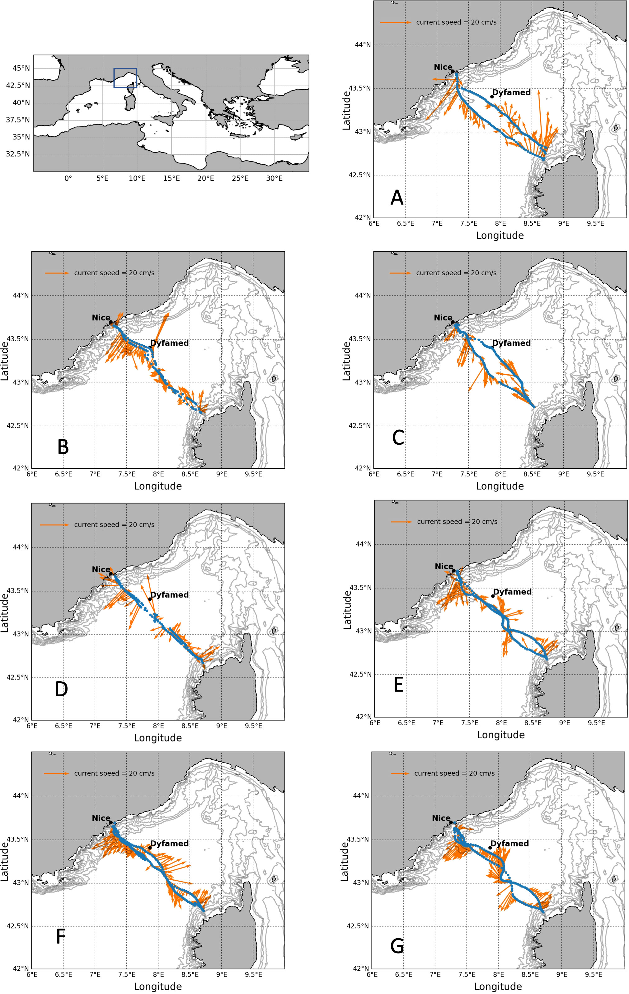
Figure 1 Glider trajectories indicated by blue dots from Nice to Calvi with the depth-average currents during the winter-spring 2018 experiment in the Ligurian Sea: (A) 11-24 January, (B) 5-13 February, (C) 20 February-5 March, (D) 14-27 March, (E) 27 March-13 April, (F) 16 April-3 May, (G) 7-23 May. Depth-average currents estimated by the glider are shown with the orange arrows.

TABLE 1

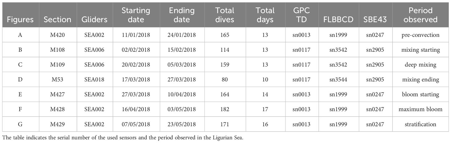
Table 1 List of the Sea-Explorer gliders sections operated along the Nice-Calvi sections from January 11^th to May 23^rd 2018.

Each section lasted between 10 and 16 days depending on weather and current conditions. The time between sections was short (2-7 days) thanks to the fast charging of the battery possible on SeaExplorer gliders but also depending on the weather conditions. An exception was observed for the section D (mission M53) which was reduced due to a technical problem on the glider. As a result, this section was not complete and represented a short trip to Calvi (reached on March 19^th) and back from Calvi to Nice on March 27^th. The distance covered by the gliders during the deployment period is shown in Figure S1. All gliders dived to 600-700 m, which represents a profile every 3-4 hours (equivalent to a horizontal distance from 3 to 5 km).

The type of payload was identical for all gliders. It was composed of a GPCTD (continuously pumped CTD at 1s) equipped with an SBE43F dissolved oxygen (DO sensor from SeaBird) and an ECO puck FLBBCD-EXP from Wetlabs (fluorescence, CDOM, backscattering) with a sampling mode at 4s. The accuracy (and corresponding resolution) of the GPCTD sensor was ± 0.002°C (0.001°C) for temperature, ± 0.003 mS cm^-1 (0.0001 mS cm^-1) for conductivity, and ± 0.1% (0.002%) of full-scale range for pressure. The SBE43F has the same accuracy as the classic SBE43 sensor (± 2% of saturation equivalent to 2 µmol kg^-1). The FLBBCD-EXP version combines the FLBB optical design with a CDOM fluorometer. The sensor measures proxies of phytoplankton abundance (chlorophyll fluorescence excitation/emission 470/695 nm with a resolution of 0.025 µg l^-1), total particle concentration (backscattering at 700 nm, resolution of 0.003 m^-1), and dissolved organic matter (CDOM fluorescence excitation/emission 370/460 nm, resolution of 0.28 ppb) in a single data stream.

The DAC had been deduced from the glider’s dead reckoning navigation and GPS fixes made at the surface. This current represents the mean current integrated over the water column after each dive (0-600m). A compass calibration has been carried out before each deployment allowing DAC to be used to reference geostrophic velocities as commonly done (Bosse et al., 2016; Bosse et al., 2017).

2.2 The glider data processing

The dataset is composed of the data corrected from the thermal lag and the sensor lag, despiked and interpolated every 1 m. A quality control (QC) with a data adjustment process has been performed when the gliders passed near the fixed station of DYFAMED (50 km from the coast; Marty, 2002) for T-S-DO and Chl-a (chlorophyll-a) measurements. The open sea site is visited every month with CTD casts and seawater sampling for biogeochemical measurements (Marty, 2002). It provided a good reference dataset to check the quality of the glider sensors (CTD-DO, FLBBCD) and to correct the possible drifts and offsets of sensors.

For the DO concentrations, the calibration coefficients of the SBE43F sensors used during the glider experiment (sn0247 and sn2905) have been adjusted (the SOC corresponds to the oxygen signal slope, the Foffset to the voltage at zero oxygen signal, and E to the pressure correction factor) based on the raw data processing algorithm (Owens and Millard, 1985) and by minimizing the sum of the square of the difference between the Winkler oxygen values (measured at the DYFAMED station during the monthly cruises) and the DO concentrations derived from the SBE43F sensor signal (Coppola et al., 2018). The total uncertainty of the adjusted DO profiles is estimated at around ± 3 µmol kg^-1. During the reference measurements at DYFAMED, the conductivity and fluorescence sensors were adjusted to correct for possible sensor drift by applying a slope and offset correction on the salinity values and by adjusting the scale factor and dark value used by the fluorescence sensor, respectively (Table S1; Figures S2–S4).

Once the dataset of each glider section has been adjusted and concatenated (homogenization of the sensor frequencies), we used the secondary QC for physics (TSO₂) and for fluorescence data described by Gregor et al. (2019). In this study, only the DO profiles of the glider descents were used for the calculations because the ascending profiles are likely to be affected by the glider turbulence on ascent.

For the TSO₂ profiles, a cleaning despiking filter was applied to remove the outliers. More specifically we used the Savitzky-Golay smoothing filter which keeps the profile shape while removing high-frequency spikes in the data. For the fluorescence data, we used three procedures to remove the bad profiles, the dark count, and the spikes. The bad profiles have been removed using a reference depth of 300 m. Then the fluorescence is averaged below 300 m and when the values are higher than the average profile (multiplied by a factor of 3), the profiles are identified as outliers. Secondly, the in situ dark count is calculated from the 95^th percentile between 300 and 400m and then removed from the fluorescence data. Finally, the data are despiked using an 11-point rolling minimum and maximum. This forms the baseline, where the spikes are the difference from the baseline. After these QC procedures, the quenched data are corrected using the methods from Lavigne et al. (2015) and Xing et al. (2012). The principle is to determine the quenching depth as the minimum depth of the smallest differences between daytime fluorescence and average night-time fluorescence. Then, the night-time backscattering ratio to fluorescence is used to correct the daytime fluorescence profile.

The data filtering and smoothing were applied to eliminate noise and short-term fluctuations in the data. This highlights longer-term spatial patterns and reduces temporal variability. Spatial interpolation in time series (sections) helped us fill in missing data points and create continuous spatial fields from discrete glider measurements. The time-series operations carried out in this study on individual glider trajectories enabled us to identify temporal variability along each trajectory.

2.3 Calculation of the net biological oxygen production (F_NCP)

The NCP is the difference between gross primary production and respiration. It represents the balance between anabolic and catabolic processes and thus between autotrophy and heterotrophy (Staehr et al., 2011). It can be estimated from the net biological oxygen production (F_NCP) and then converted to carbon production (NCP) with a fixed oxygen-to-carbon ratio of 1.45 (Hedges et al., 2002). Although a lower O₂:C ratio was recently observed by Hemming et al. (2022), their ratio was only estimated for 25 days in March 2016 which is too short to be used in this study which covers a more extended period. In this case, we prefer to use the classic Hedges ratio used in the literature.

The change in DO concentrations over time is due to biological (respiration, photosynthesis) and physical processes (dissolution of air, bubble injection, changes in water temperature and air pressure). To calculate the F_NCP from gliders, we used the same methods used by Binetti et al. (2020) and Possenti et al. (2021). The method is described in Figure 2. It is based on the mass balance of DO in the mixed layer equivalent to the changes in the DO inventory per unit area in the upper ocean (I_O2), the air-water gas exchange of oxygen (F_aw), the entrainment of the DO flux with the mixed layer depth deepening (F_ent) and the diapycnal eddy diffusion flux (F_d). Horizontal advection transport was not considered in this study because the horizontal gradients of the surface oxygen saturation anomaly are small and the surface oxygen concentration is reset by air-water gas exchange in a relatively short period of time (Yang, 2021). For the calculation of the different DO fluxes, profiles have been interpolated every 3h after removing the outliers.

FIGURE 2

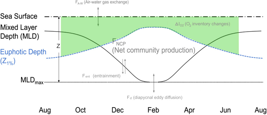
Figure 2 Schematic representation of the net biological oxygen production (F_NCP) fluxes in the upper surface over the year (modified from Yang, 2021). ΔI_O2 represents the change of O₂ inventory between consecutive profiles (above Zeu), F_aw the air-sea O₂ flux using the method of bubble injection from Woolf and Thorpe (1991), F_ent the entrainment of O₂ concentrations when MLD deepens (Z_MLD below Z_eu) and F_d the diapycnal eddy diffusion flux.

The F_NCP is calculated from the following equation:

$$F_{NCP}=\mathrm{\Delta }{I}_{O2 }+F_{aw}-F_{ent }-F_{d }$$

F_aw (mmol m^-2 d^-1) was calculated using the method of bubble injection from Woolf and Thorpe (Woolf and Thorpe, 1991)

$$F_{aw}=k_{O2} \times [O_{2sw}-(1+\Delta )\times O_{2sat}]$$

where k_O2 (m s^-1) is the gas transfer velocity for oxygen, O_2sat the oxygen saturation, O_2sw is the oxygen concentration above 10 m, and $\Delta$ the bubble injection correction (Atamanchuk et al., 2020). The estimation of k_O2 was identical to those used in Coppola et al. (2018) with a wind speed measured by the ODAS buoy at the DYFAMED site (Côte d’Azur from Météo France). During the study period, the wind speed was lower than 19 m s^-1. The bubble correction represents the normalization of the wind speed at 9 m s^-1 when the oxygen concentration is supposed to be 1% supersaturated (Woolf and Thorpe, 1991).

ΔI_O2 (mmol m^-² d^-1) is the change of DO inventory between consecutive profiles in the upper layer. The DO inventory (IO₂) was calculated as the DO concentrations integrated above the euphotic layer (Z_eu).

$$\mathrm{\Delta }{I}_{O2}= \frac{[I{O}_2(t_2)-I{O}_2(t_1)]\times Z_{eu}}{(t_2-t_1)}$$

with

$$I{O}_2= \frac{{\int }_0^{Zeu}\mathrm{\Delta }{I}_{O2}}{Z_{eu}}$$

F_ent (mmol m^-² d^-1) corresponds to the change of DO concentrations when the mixing process is intense or in other words when the mixed layer deepens below Z_eu. In this study, Z_eu has been estimated using the method of Morel and Berthon (Morel and Berthon, 2003), and the mean euphotic depth was estimated at around 50 m. The depth of the mixed layer (Z_mld) was calculated as the depth where the potential density difference from the surface reference depth (10 m) was close to 0.03 kg m^-3 (de Boyer Montégut et al., 2004; D'Ortenzio et al., 2005). F_ent could be positive if there is an increase in the oxygen inventory. If Z_mld is above Z_eu, F_ent is negligible.

$$F_{ent}= \frac{[I{O}_2(z_{mld} , t_2)\times (\frac{Z_{eu}}{Z_{mld}})- I{O}_2(z_{eu} ,t_1)]}{t_2-t_1}$$

F_d was calculated at Z_mld when it was deeper than Z_eu and at Z_eu when Z_mld was shallower than Z_eu

$$F_d= K_{z }\times \frac{\partial O_2}{\partial z}$$

with a vertical eddy diffusivity K_z of 10^-5 m² s^-1 for the NW Mediterranean basin (Ferron et al., 2017).

Uncertainty about F_NCP derives from the total propagated error of each flux used to calculate the NCP flux (Hemming et al., 2022). The uncertainties of ΔI_O2, F_ent, and F_d correspond to the standard error of glider profiles (DO adjustment error). For F_aw, it includes the same standard error plus 20% of the uncertainty in the gas transfer velocity (Wanninkhof, 2014).

2.4 Calculation of the air-sea CO₂ exchanges from the gliders and CANYON-MED

The air-sea CO₂ exchange fluxes (F_CO2) were calculated from the difference between the partial pressure of CO₂ measured in the seawater (pCO_2sw) and in the atmosphere (pCO_2atm).

The pCO_2sw were based on the predictions of the CANYON-MED neural network using adjusted T, S, DO measured by the gliders at 10m depth as input variables (Fourrier et al., 2020). The neural network (NN) CANYON (CArbonate system and Nutrients concentration from hYdrological properties and Oxygen using a Neural network) is based on techniques derived from artificial intelligence to provide several unmeasured biogeochemical variables with good accuracy such as nutrients, pH, and pCO₂ (Sauzède et al., 2017; Bittig et al., 2018). Here, we used a regional version of CANYON developed for the Mediterranean Sea (CANYON-MED) to predict nutrients and carbonate variables from pressure, temperature, salinity, and oxygen together (with geolocation and date of sampling) measured in the water column by different autonomous platforms (mooring, Argo floats) and ship visits (Fourrier et al., 2020). To improve the accuracy of the predicted variables, an ensemble of ten NN has been proposed (one for each variable) and recently applied in the northwestern Mediterranean Sea (Fourrier et al., 2022) to estimate the trends of nutrients and CO₂ variables (Total Alkalinity or TA, Dissolved Inorganic Carbon or DIC, pH) from surface to deep waters. In this study, the pCO_2sw was derived from DIC and pH at the total scale predicted by CANYON-MED and the CO2SYS v3.0 Matlab toolbox (Sharp et al., 2020).

The pCO_2atm was estimated from the dry mole fraction of CO₂ (xCO₂) measured at the OHP atmospheric station (Observatoire de Haute Provence, St Michel l’Observatoire, France) and the vapor pressure formula proposed by Ambrose & Lawrenson (1972), then corrected by Millero and Leung (1976). The Corsica station (ERSA) is closer to the study site but data was not available before March 2018. In addition, the comparison of pCO_2atm data between the OHP station and ERSA is quite close (less than 1 µatm on average), which suggests that the data from the OHP station are consistent with our study area.

F_CO2 (mmol m^-2 d^-1) is determined according to the equation:

$${\text{F}}_{\text{CO}2}=\text{k}\times \mathrm{\alpha }\times (\text{pC}{\text{O}}_{2\text{SW}}-\text{pC}{\text{O}}_{2\text{atm}})$$

where k is the gas transfer velocity of CO₂ according to Wanninkhof (2014) in cm h^-1 and 𝛂 is the solubility function of CO₂ (in mol L^-1 atm^-1) from Weiss (1974). The k factor is calculated using the formula:

$$\text{k}=0.251\times {\text{U}}_{10}{2}^{}\times {(\text{Sc}/660)}^{0.5}$$

where U10 is the wind speed (m s^-1) measured at the ODAS buoy at DYFAMED (Météo France) and Sc the Schmidt number (no dimension) determined according to the equation of Wanninkhof (2014).

Uncertainty in the air-sea CO₂ flux corresponds to the 20% uncertainty in k (Wanninkhof, 2014) and the uncertainty of predicted pCO_2sw is based on the root mean square error of predicted DIC (12.35 µmol kg^-1) and pH (0.0156) of CANYON-MED for the western Mediterranean Sea (Fourrier et al., 2020). The error package of the CO2SYS v3.0 toolbox (Orr et al., 2018) provided a pCO_2sw uncertainty estimated to 15 µatm using constants K1 and K2 from Mehrbach et al. (1973) as refitted by Dickson and Millero (1987) and the dissociation constant for HSO₄ form Dickson (1990). Finally, as the uncertainty of pCO₂ is dominated by the uncertainty in estimated pCO_2sw, the small contribution from atmospheric CO₂ is neglected (less than 1 μatm; Landschützer et al., 2014).

3 Results

3.1 Physical and biogeochemical seasonal time series

Each glider section (seven in total noted A to G) represents a roundtrip from Nice to Calvi passing through the DYFAMED site located in the central zone of the Ligurian Sea (Figure 1). Near the coast, the presence of the Northern Current (NC) results from the cyclonic circulation in the northwestern basin, which flows along the Ligurian to Catalan coasts, 30 km wide and up to 250 m deep (Millot, 1999). In the Ligurian Sea, it results in a permanent structure called the Ligurian front jet which usually delimits the coastal waters from denser waters of the central Ligurian Sea (Astraldi and Gasparini, 1994; Millot and Taupier-Letage, 2005). During the study period, the NC was located around 15 km off the French coast, with a mean horizontal velocity of 15 cm s^-1 minimum and 45 cm s^-1 maximum in winter, which is consistent with previous observations (sections A and B). The Western Corsican Current (WCC), one branch feeding the NC, is located in the north of Corsica and characterized by higher salinity with lower current velocity than the NC. In this study, the WCC was observed during all transects and was particularly intense in January (section A).

The TSO₂ time series over the A to G sections are represented for downcast 0-600m profiles after data processing with Z_mld values (Figure 3). From 11 to 23 January (section A), warmer waters were located near the coast in Nice and Calvi (above 14°C) and colder in the central zone of the Ligurian Sea (13-13.5°C). The deepest Z_mld observed was estimated at around 200 m. The salinity was lower near the coast and above the Z_mld in the central zone (38-38.4) while high salinity was measured below in the intermediate water (38.5-38.6). On the contrary, oxygen concentrations were higher above the Z_MLD in the entire area (240-260 µmol kg^-1) and lower below 300m (170-180 µmol kg^-1).

FIGURE 3

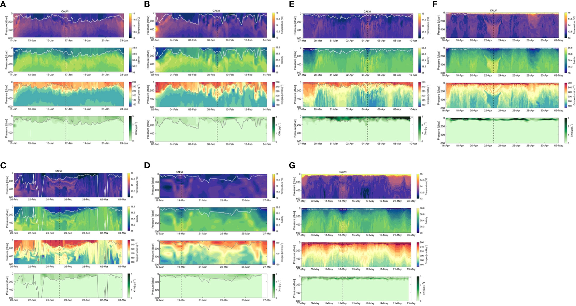
Figure 3 Time evolution of temperature, salinity, dissolved oxygen (µmol/kg) and Chl-a (µg/L) with the position of the Mixed Layer Depth (MLD, m) indicated by the white line along the Nice-Calvi sections during the 7 Sea-Explorer deployments: (A) 11-24 January, (B) 5-13 February, (C) 20 February-5 March, (D) 14-27 March, (E) 27 March-13 April, (F) 16 April-3 May, (G) 7-23 May. All sections start and end at Nice while the location of Calvi is indicated by the black dashed line.

In February (sections B and C), colder water rapidly invaded the area (13-13.5°C) with deepening of the Z_mld reaching its maximum (below 600m) in the central zone on 22-23^rd February and on 1-2^nd March. The salinity was still low at the surface in February but increased rapidly at the surface during the intense vertical mixing (deepest Z_mld with 38.6 at the surface). After mid-February, the oxygen minimum in the intermediate water was mitigated due to the influx of DO-rich surface water during vertical mixing (190-200 µmol kg^-1). TSO₂ homogeneous profiles were observed during the second deepest Z_mld event in early March near the DYFAMED site (Figure 3C).

After mid-March until early April (sections D and E), cold waters were still present in the whole area and the water column and the Z_mld shallowed from 250 to 150 m in the central zone. Some lower salinity appeared at the surface, especially near the coasts. During this period, DO concentrations were again higher at the surface while in the intermediate waters DO concentrations were heterogeneous, ranging from 180 to 200 µmol kg^-1.

From mid-April to the end of May, the stratification appeared with higher temperature, lower salinity, and high DO concentrations at the surface. In the intermediate water, a maximum of salinity was observed in Calvi and lower DO concentrations slowly settled below 300 m.

3.2 Spatial and temporal variability observed using glider data

Deconvolution of the temporal versus spatial variability from glider data have been already investigated (Rudnick and Cole, 2011; Piterbarg et al., 2014; Little et al., 2018). This phenomenon is not specific to glider data but affects all oceanic lagrangian platforms (Argo floats, surface drones, ships and satellites). Some methods have been developed and applied to limit the problem.

For example, in the Ligurian Sea, mesoscale variability of the NC has been studied using repeated glider sections from Nice to DYFAMED to investigate the propagation of the velocities (Piterbarg et al., 2014). They suggested that temporal variability can appear in glider data as integrated with spatial variability through the Doppler friction mechanism. To illustrate the effects of spatial and temporal variability, they proposed to investigate the time scales of the NC front that can vary significantly over the 6-7 sampling days, so that the spatial variability recorded by the gliders may be at least partially due to temporal variability. To deconvolute the spatial and scale variability of the system, they proposed to estimate the time dependence of a the representative isopycnals of the front (29.05 kg/m³).

In this study, gliders moved horizontally at a speed of around 1 km/h (or 0.5 knt) with constant vertical profiles from the surface to 600-700 m, and each section represented a round trip between Nice to Calvi. For comparison with the study of Piterbarg et al. (2014), we applied the same method to test how the gliders observed the variability of NC front (Figure S5). The results show a mesoscale signal with scales consistent with a cross-shore oscillation of the front between around 15 and 50-60 km offshore, which is consistent with the literature (Prieur, 1979). We observed that the NC front oscillation was fairly smooth during sections A, E, F and G, with a propagation speed (2 km/day) significantly lower than that of the glider speed (1 km/h), so that the processes observed on the outward section did not change position on the return section. During sections B and C (as section D was truncated, the propagation speed of the front cannot be assessed), the system undergoes more rapid changes with time scales of the order of 4-5 km/day, but it also remains below the speed of the glider.

Regarding the variability of biogeochemical variables in the NW Mediterranean Sea, the time scale can go from days to months. Spatial scales of variability were mostly small at depths affected by biology, and large at depths affected by large scale processes, such as deep convection and ventilation. Small scale structures can affect the DO and Chl-a content (Niewiadomska et al., 2008; Bosse et al., 2017) and data recorded from the gliders are usually completed by satellite observation (SST, ocean color) to estimate the spatial and temporal variability. In this study, although some spatial contrasts were observed between coastal and offshore waters, a consistent temporal pattern can be observed for glider DO concentrations between the Nice to Calvi and Calvi to Nice sections (Figure 3). These consistent temporal patterns across the section suggest relative spatial homogeneity, and although small structures may affect DO concentrations locally, we can assume that temporal variability is predominant in interpreting the change in DO content between sections.

3.3 Chl-a content variability

The spring bloom began in late March and ended in late April (sections E and F in Figures 3, 4). The maximum integrated Chl-a in the Z_mld was observed on April 9^th and was estimated at around 4 µg L^-1 which is consistent with previous studies in the Ligurian Sea (Lavigne et al., 2015; Mayot et al., 2017). The spatial distribution of surface Chl-a from the MODIS observation (daily data, resolution 1 km) showed an onset near Calvi during section D (March 14 to 27; Figure 5). The maximum Chl-a concentration was observed during section E (March 27 to April 13) and occurred mainly in the central Ligurian Sea area (Figures 3D, E, 4) with a range from 4 to 5 µg L^-1 during the section E which is consistent with the glider measurements.

FIGURE 4

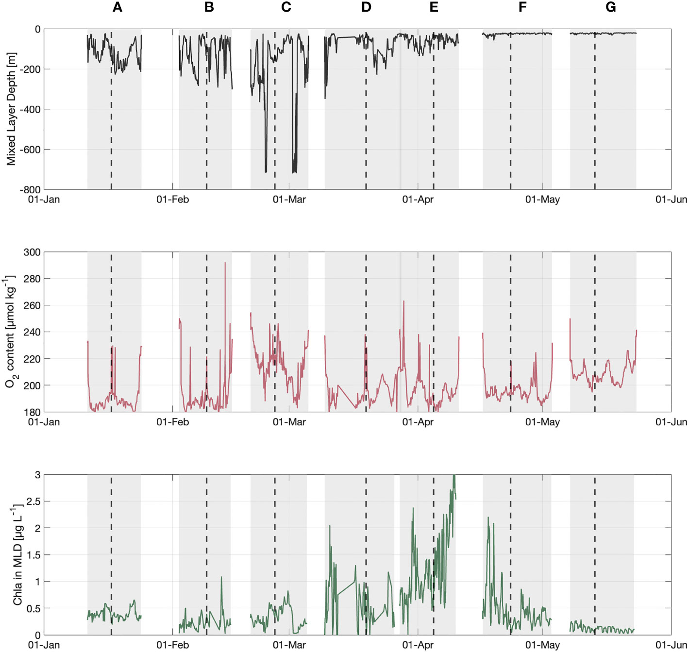
Figure 4 Time series of the MLD (m), the content of oxygen and Chl-a integrated in the MLD during the all period of gliders deployment. Each section is represented by a grey area (round trip Nice-Calvi). The label of the sections is similar to the Figure 2. The dashed line represents the position of Calvi.

FIGURE 5

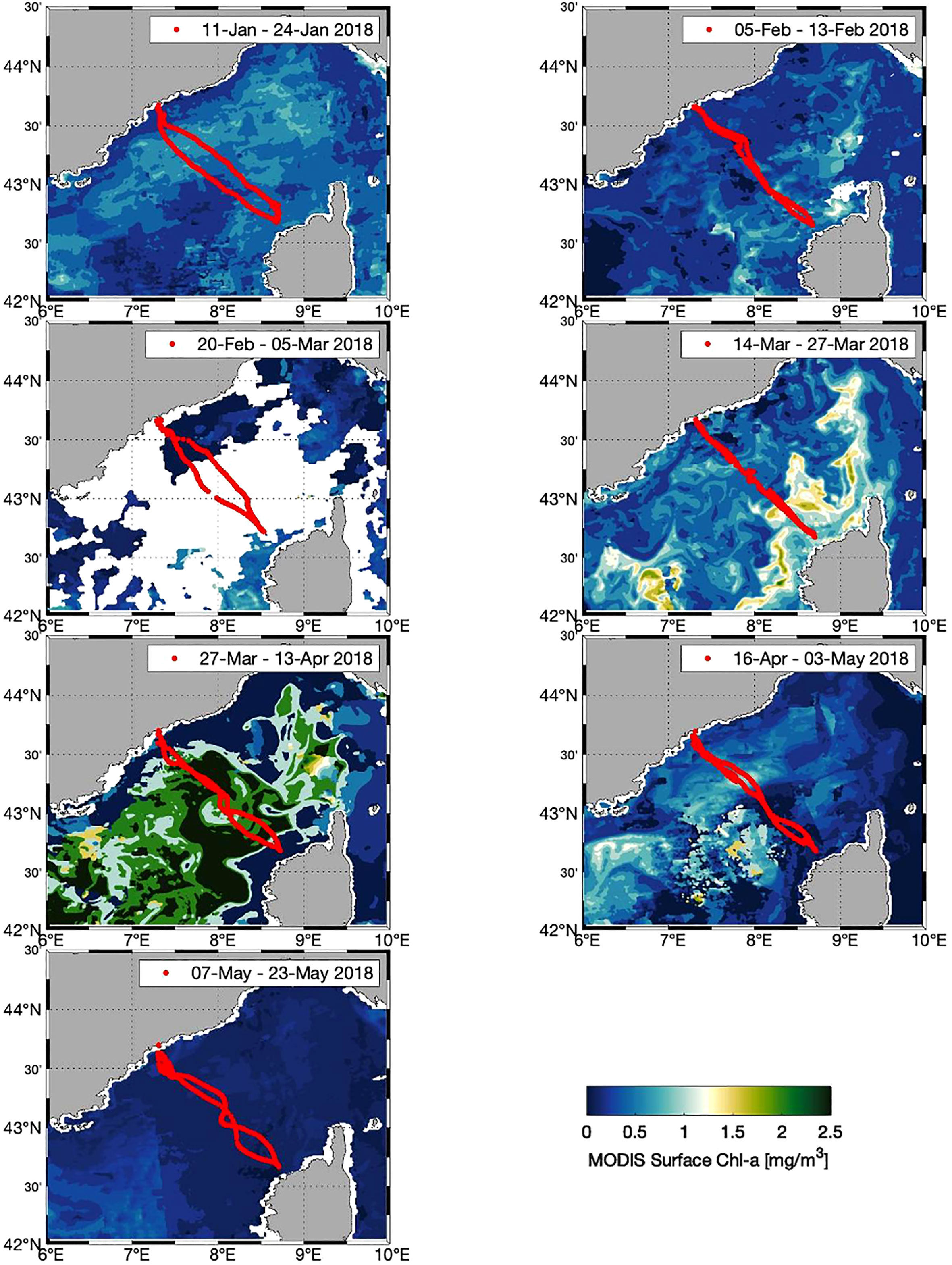
Figure 5 Glider trajectories indicated (red dots) with the surface chlorophyll-a concentrations from ocean color satellite observations (MODIS) during the 7 Sea-Explorer deployments (images from ACRI-ST L3 daily 1 km resolution; GlobColour daily merged MODIS/VIIRSN product).

3.4 The depth limits and the oxygen production

The F_NCP calculation is based on DO integration above the depth limits Z_mld and Z_eu. The Z_mld was high during sections (or period) B and C (from February to early March) and it reached its maximum (deeper than 600m) on February 23 and March 2 in the central zone of the Ligurian Sea (Figure 6). After this mixing period, the Z_mld ranged from 100 to 200 m in section D and E (mid-March to mid-April). From sections A to E, Z_mld was below Z_eu and the depth of the Deep Chlorophyll Maximum (Z_dcm). At the end of the bloom and during the stratification period (sections F & G, mid-April to end of May), Z_mld was shallow (about 20-25 m) and Z_eu and Z_dcm were deeper than Z_mld and mostly equivalent (around 50 m).

FIGURE 6

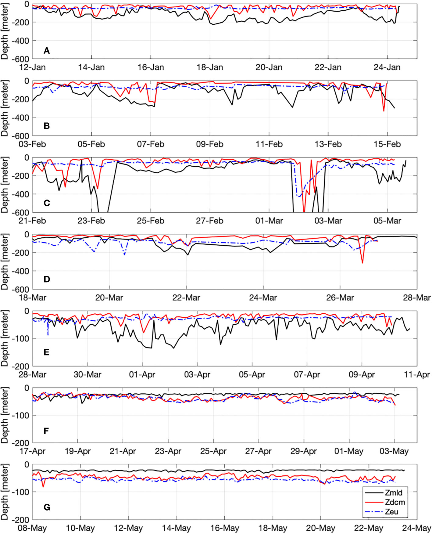
Figure 6 Evolution of the euphotic depth (Z_eu), mixed layer and deep chlorophyll maximum depth (Z_mld and Z_dcm, respectively) over the glider deployments. Labels (A–G) represent the different sections from January to the end of May 2018.

The time series of Z_eu and Z_dcm, showed that Z_eu remained largely constant during the study period (around 50 m) while Z_dcm was strongly influenced by the variability of the Z_mld (Figure 6). The main reason is due to the mixing event which induced a supply of nutrients to the surface and a vertical dilution of the phytoplankton species from surface to deep waters (Mignot et al., 2014; Cornec et al., 2021).

F_aw showed a trend influenced by the wind conditions with negative values from sections A to E indicating an influx from the atmosphere into seawater or DO uptake (Figure 7). This is caused by low sea surface temperature and surface water undersaturated in oxygen (80-100%) from mid-January to early April. The minimum F_aw value (-692 ± 138 mmol m^-2 d^-1) was observed on March 2^nd when the observed heat flux loss was the highest. It corresponds to the coldest air temperature (2°C) and peak wind speed (20 m s^-1) recorded at the DYFAMED site (Figure 8). After this date, F_aw was lower but still negative. It decreased to -416 ± 83 mmol m^-2 d^-1 between March 20-22 when the mixed layer deepened, the surface salinity increased and the surface DO concentration decreased (Figure 7D). After the winter period, F_aw increased slowly and the flux was positive up to 100 ± 20 mmol m^-2 d^-1 in mid-May. This outflow of DO from the sea to the atmosphere was consistent with stratified, warmer, and oxygen-saturated surface waters occurring during this period of the year in the Ligurian Sea (Coppola et al., 2018).

FIGURE 7

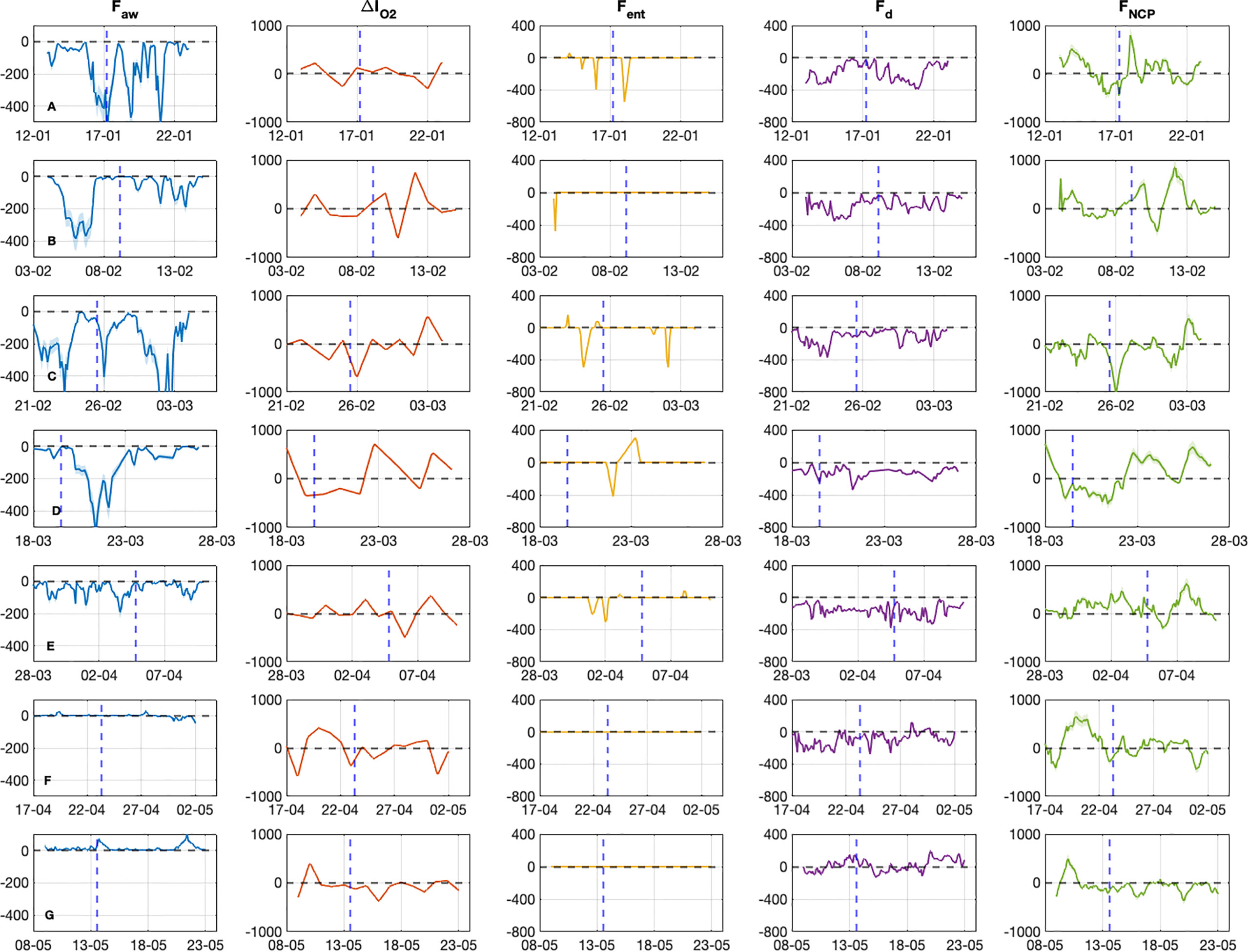
Figure 7 Time evolution of the O₂ fluxes (mmol/m2/d) used for the F_NCP estimation during the 7 glider sections. F_aw represents the air-sea flux exchanges, ΔI_O2 the change of O₂ inventory above Z_eu and between consecutive profiles and F_ent the entrainment of O₂ concentrations when MLD deepens and F_d the diapycnal eddy diffusion flux. The blue dashed line represents the position of Calvi. All fluxes are expressed in mmol/m²/d. Labels (A–G) represent the different sections from January to the end of May 2018.

FIGURE 8

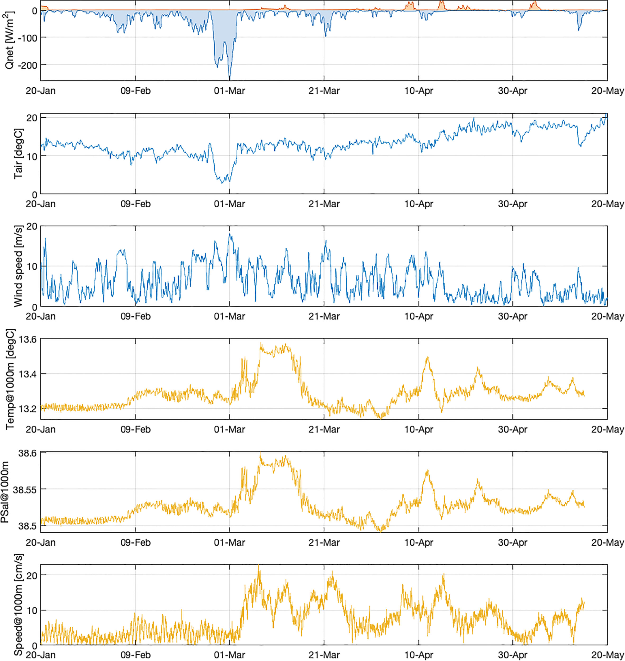
Figure 8 Meteorological and oceanic observations in the DYFAMED site from 20 January to 20 May 2018 (blue and yellow lines, respectively). First panel: the blue color in the heat flux (Qnet) indicates a loss of heat while the red color indicates a heat gain (Meteo France data). The oceanic measurements are collected at 1000m depth from October 2017 to May 2018 indicated the variability of in situ temperature, salinity and current speed (EMSO data).

The DO inventory (ΔI_O2) in the euphotic zone was high (-681 ± 12 to 744 ± 15 mmol m^-2 d^-1) and very variable during the mixing period (sections B to D) when the glider passed through different mixed and unmixed areas from Nice to Calvi. This is typical of a dynamic situation because the DO content is mainly determined by the mixing process in winter (Coppola et al., 2017). During the stratification period, the oxygen stock was lower and ranged from -370 ± 6 to 393 ± 7 mmol m^-2 d^-1 (Figure 7G).

The change of oxygen concentration due to entrainment to deep water (F_ent) was significant at sections A, C, and D when the mixed layer deepened. It was especially intense (-500 ± 9 mmol m^-2 d^-1) when the deepest Z_mld was observed from Nice-Calvi at the end of February and in early March. After March, the entrainment was negligible due to the stratification conditions.

F_d ranged from -390 ± 6 to 189 ± 2 mmol m^-2 d^-1 from January to May with negative values in the central zone of the section Nice-Calvi from January to April and slightly positive in May.

Finally, the F_NCP and NCP were very variable due to the dynamics of the Ligurian Sea (Figures 7, 9): the fluxes oscillated from negative to positive values in winter ranging from -1022 ± 206 to 803 ± 161 mmol m^-2 d^-1 (equivalent to -705 ± 142 to 554 ± 111 mmol m^-2 d^-1). In spring, the positive fluxes were more predominant ranging from -432 ± 87 to 642 ± 129 mmol m^-2 d^-1 (equivalent to -298 ± 60 to 443 ± 89 mmol m^-2 d^-1). The average of NCP during the experiment was equivalent to 0.33 gC m^-2 d^-1.

FIGURE 9

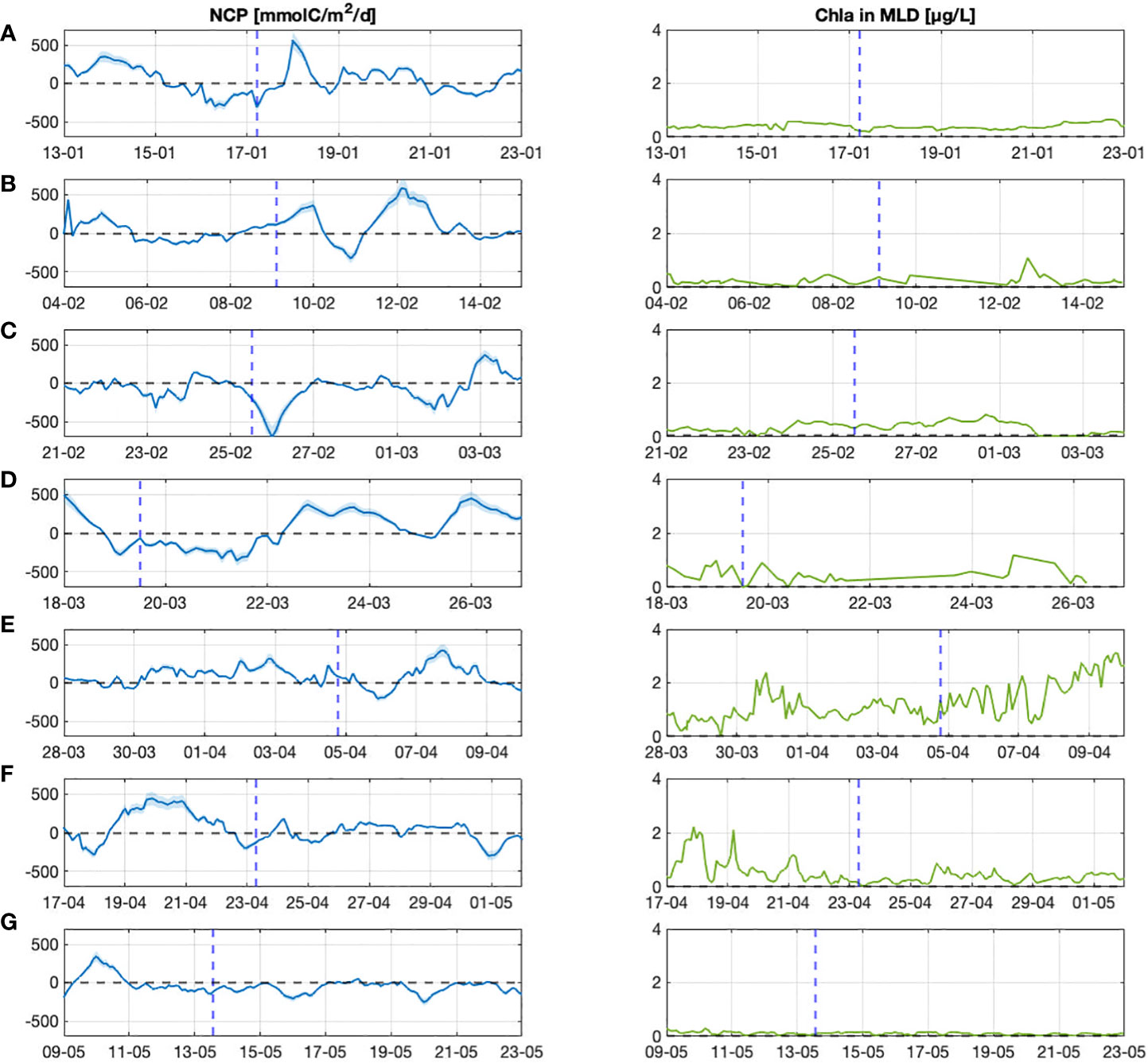
Figure 9 Seasonality of the NCP flux and Chl-a content in the MLD layer during the glider experiment (autotrophic vs. heterotrophic situation). Labels (A–G) represent the different sections from January to the end of May 2018.

3.5 The CO₂ fluxes at the air-sea interface

Estimates from CANYON-MED and glider data show pCO₂ in seawater and in atmosphere ranging from 362 to 437 µatm and from 400 to 439 µatm, respectively (Figure 10, left panel). Based on pCO₂ and the equation defined in 2.4, we estimated an air-sea CO₂ flux ranging from -16.5 ± 3.9 to +7.8 ± 1.9 mmol m^-2 d^-1 from Nice to Calvi from January to May 2018 (Figure 10, right panel). By convention, negative CO₂ fluxes indicate a CO₂ uptake from the atmosphere to the seawater. Our estimate is consistent with negative flux (CO₂ sink) in winter (February-March) when the deep convection and under-saturation of CO₂ at the surface induced absorption of atmospheric CO₂ in the central zone of the Ligurian Sea. Air-sea CO₂ flux showed positive values near the coast and during May but over the entire spring period, the central zone of the Ligurian still absorbed some atmospheric CO₂.

FIGURE 10

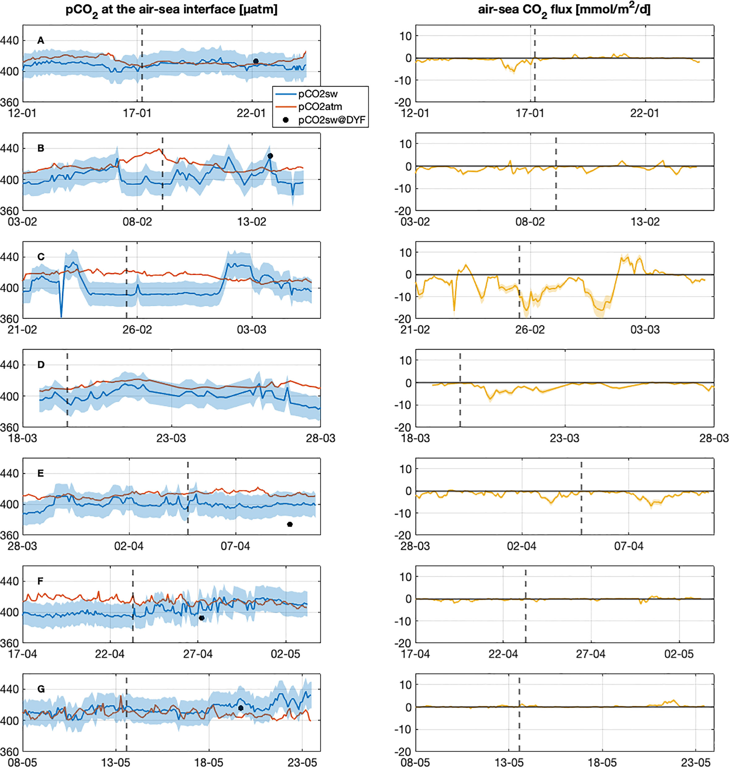
Figure 10 Left panel: time series of pCO₂ (µatm) measured in atmosphere (OHP station) and in seawater using the predictions of the neural network CANYON-MED (Fourrier et al., 2020) based on glider measurements along the sections. The black dots represent the in-situ measurements of pCO₂ in DYFAMED buoy and the blue dashed area the pCO₂sw uncertainty. Right panel: air-sea CO₂ flux estimated from pCO₂ in atmosphere and in seawater along the glider sections. The yellow dashed area corresponds to the CO₂ flux uncertainty. The dashed line represents the position of Calvi. Labels (A–G) represent the different sections from January to the end of May 2018.

4 Discussion

4.1 The last deep convection event observed in the Ligurian Sea

In the Mediterranean Sea, the deep-water formation (DWF) is due to evaporation and the difference in temperature between the air and the relatively warm surface waters (13°C). In the northwestern basin, this evaporation and heat loss is accentuated by the strong, cold, dry winds (Mistral, Tramontane) that prevail in winter in the Gulf of Lion and sometimes extend to the Ligurian Sea when winters are particularly severe (Houpert et al., 2016). In the past (2005/2006 and 2012/2013), extremely cold winters induced intense deep convection in this region with massive vertical transport of heat and salt to the deep waters with the appearance of warmer, denser, and O₂-rich deep waters (Schroeder et al., 2008; Smith et al., 2008; Marty and Chiavérini, 2010; Coppola et al., 2018; Testor et al., 2018). This intense vertical transport induced a significant input of oxygen into intermediate waters (mainly the Levantine Intermediate Water or LIW) which is characterized by lower DO concentrations with an important signature in the Ligurian Sea (Coppola et al., 2017; Coppola et al., 2018). These intense DWF also induced important nutrient supply in the upper layer resulting in intense phytoplankton production with a large export of organic carbon to deep waters (Pasqueron de Fommervault et al., 2015; Mayot et al., 2017; Kessouri et al., 2018).

Since 2014, no intense DWF events have been observed from long-term observation platforms. These events are likely to have been influenced by climate change during the 21^st century (Somot et al., 2006; Adloff et al., 2015) and by natural variability, such as decadal variability in the characteristics of the Atlantic inflow or mixing with saltier and warmer Mediterranean outflow water at the Strait of Gibraltar (Millot, 2007; Somot et al., 2016). Consequently, during the period 2014-2018, warmer and saltier LIW then accumulated in the northwestern basin in the absence of intense DWF until 2018, which could trigger the next massive deep convection if external forcings (e.g., winds) occur (Margirier et al., 2020).

During the winter of 2018, we observed intense heat loss, strong northeast wind, and cold air temperature in the Ligurian Sea in early March (Figure 8). As expected, it induced an intense vertical mixing measured until 1000m at the EMSO-DYFAMED mooring several days after this atmospheric event (Coppola et al., 2023). In parallel, gliders deployed in the Ligurian have confirmed this observation with an estimated Z_mld of 600 m (the maximum depth limit of sensors) on Feb. 23^rd and on March 1^st near the DYFAMED site (Figure 3C).

This event produced an intense mixed layer deepening with strong DO ventilation observed in February-March 2018 (sections B and C in Figure 3) which was more intense compared to the period 2014-2017 in the Ligurian Sea (Margirier et al., 2020). DO concentrations increased from 20-40 µmol kg^-1 when Z_mld was maximum (more than 700m) at the end of February and in early March. This deep mixing then induced a large amount of oxygen ventilation altering the DO minimum signal usually observed in the LIW depth range and a dilution of low Chl-a concentrations.

It is therefore interesting to understand how this intense mixing may have impacted the oxygen production and the NCP, as well as the ecosystem response to this intense disturbance. Indeed, in early March, the most negative value of F_aw has been estimated in the central zone of the Ligurian Sea with an increase of DO content and a high entrainment flux suggesting a large DO uptake into the surface waters (Figures 3, 7). This result confirms that strong air-sea transfer of O₂ (strong winds) is accompanied by an opposing increase in the MLD (due to intense mixing) and changes in DO inventory. On the other hand, this event has a low impact on oxygen production due to positive values of I_O2 which correspond to rapid changes of DO inventory and the complexity of the mixed patch during DWF delineating the water column cells with ventilated and non-ventilated water masses.

4.2 Impacts on NCP and Chl-a content

Calculating NCP from glider data is challenging because the glider is constantly moving through different water masses and from the coastal to open sea waters with sub-mesoscale structures (Niewiadomska et al., 2008). Indeed, rapid and strong bloom patches with meanders and sub-mesoscale structures have been observed with the MODIS satellite (Figure 5) and in the previous glider experiments in the area (Bosse et al., 2016; Bosse et al., 2017). Moreover, the influence of complex processes occurring in the coastal waters (e.g., frontal upwelling and downwelling processes, coastal river plumes) could explain extreme NCP values near Calvi and Nice in sections B and C (Figures 7, 9).

Based on the gliders speed (see section 3.2), we observed a mixed layer depth (the main physical process occurring from February to the end of March) almost equivalent in the outward and return directions, suggesting that the characteristics were not different between outward and return with a central zone characterized by colder and more ventilated water compared to the coastal zones near Nice and Calvi, as already observed by Niewiadomska et al. (2008) (Figures 3, 4). In this context, we can assume that the data synopticity was adapted to capture the spatial coverage of O₂ fluxes and had low impact on the NCP estimate, especially in the central zone which corresponds to 80% of the spatial coverage of the sections. However, in this study, the small-scale unresolved spatial variations in biogeochemical variables generated by fine vertical structures are suspected and have been ignored (such as small coherent eddies or upwelling/downwelling features across the NC and WCC frontal zones observed by Bosse et al., 2016; Bosse et al., 2017). Consequently, to reduce the impact of this small-scale variability in biogeochemical variables, data processing strategies have been applied to separate spatio-temporal elements and estimate temporal evolution on spatial contributions (section 2.2). Finally, in this study, each section represents the spatial evolution along a coastal-open sea continuum bounded on both sides by a (sub-sampled) coastal frontal zone, and that the difference between each section represents the temporal evolution of O₂ content and NCP flux in the same area.

The Figure 9 indicates that heterotrophic condition was predominant until mid-March (negative NCP) while during the spring (sections D to G), NCP were positive or close to zero corresponding to an autotrophic situation. However, there was no clear relationship between NCP and Chl-a content within the mixed layer, which increased during the spring bloom (section E). This indicates that the contribution of biological production to NCP during this experiment was small, while the main component of NCP changes was air-sea flux (F_aw) in winter and DO inventory in spring.

Based on a biogeochemical and regional model (SYMPHONIE Eco3M-S), the northwestern Mediterranean Basin is found to be an autotrophic ecosystem with an annual NCP (in the upper 150 m layer) estimated at 47 gC m^-2 yr^-1 (Ulses et al., 2022). In this study, our observations estimated a higher average NCP of 27.9 ± 6 mmol m^-2 d^-1 in the Ligurian Sea (equivalent to 0.33 ± 0.07 gC m^-2 d^-1 or extrapolated for the year to 122 ± 26 gC m^-2 yr^-1) from January to May, during the most dynamic and biologically active months in terms of organic carbon production and export. We can also mention that upwelling and downwelling processes of frontal waters (e.g., isopycnal tongues of high fluorescence and oxygen concentration) could have induced local anomalies easily captured during the glider transects in this study and subsequently influencing the NCP values (Niewiadomska et al., 2008).

At the DYFAMED site, our NCP flux ranged from -292 to 415 mmol m^-2 d^-1 from January to the end of May 2018. This result is higher than previous observations based on annual measurements over 20 years estimating an NCP of 19.5 mmol m^-2 d^-1 (Coppola et al., 2018) as well as a more recent study based on glider DIC measurements in March-April 2016 that determined a NCP of 44 to 85 mmol m^-2 d^-1 (Hemming et al., 2022). This is primarily due to the fact that our observation occurred during the last year of unusually intense convection followed by a strong phytoplankton bloom. The result is a very active mixing area in the central zone of the Ligurian Sea with very high DO content in the mixing layer, likely followed by nutrient input to the surface, all accompanied by sub-mesoscale structures and frontal meanders that make the NCP values higher but highly variable at a single fixed station.

4.3 NCP and air-sea CO₂ exchanges

The Ligurian Sea was found to be a medium to minor annual sink for atmospheric CO₂ (Hood and Merlivat, 2001; Copin-Montégut et al., 2004; Merlivat et al., 2018). Previous studies at the DYFAMED site observed that the annual average CO₂ flux was estimated at 0.9 mmol m^-2 d^-1 from February 1998 to January 1999, and 1.9 mmol m^-2 d^-1 from February 1999 to January 2000 (Copin-Montégut et al., 2004). During the period 2013-2015, Merlivat et al. (2018) measured an air-sea CO₂ flux of -0.45 mol m^-2 yr^-1 which is equivalent to -1.2 mmol m^-2 d^-1. These previous observations are consistent with our study and the mean air-sea CO₂ flux predicted from January to May 2018 estimated at -1.1 ± 0.27 mmol m^-2 d^-1 in the Ligurian Sea (interpolated data). These results are also consistent with the latest model outputs from SYMPHONIE Eco3M-S capable of simulating air-sea fluxes of CO₂ in the northwestern Mediterranean Sea (Ulses et al., 2022). The model showed that the minimum CO₂ flux occurs in winter and becomes positive in summer. They estimated an annual flux of -0.4 TgC yr^-1 for the period 2012-2013 (equivalent to -1.3 mmol m^-2 d^-1) in the northwestern region. During this convective year, they estimated an annual flux of -0.33 mol m^-2 yr^-1 (equivalent to -0.9 mmol m^-2 d^-1) at DYFAMED for the period 2012-2013 which is consistent with our values.

Finally, our results demonstrate during the exceptional convection year of 2018, the capacity of the central zone of the Ligurian Sea to be a sink of CO₂ in winter could be important and associated with strong northeast winds and undersaturation of DIC at the surface. It also confirms the crucial role played by physical forcing in the DIC budget in this dynamic region.

Our study highlights that the convection process in the Ligurian Sea acts as an autotrophic ecosystem with the predominance of production over respiration, with some heterotrophic presence in the coastal waters. In general, an autotrophic ecosystem (positive NCP) is associated with a CO₂ sink (negative F_CO2). Although our estimates of NCP are 10-20 times higher than CO₂ fluxes, this concept appears to be observed in our study in late March and early April when the bloom is active but with some opposite trend: negative NCP fluxes (heterotrophic state) are associated with a CO₂ sink for the atmosphere. This discrepancy was also observed by Wimart-Rousseau et al. (2020) in the coastal waters in the Bay of Marseille. They suggested that the main reason might be due to temperature changes affecting the pCO₂ of seawater. In our study, thermal variability from January to late May was important, especially in our glider experiment-based study where coastal and open ocean waters were sampled continuously with large temperature gradients.

In our DIC predictions, we were not able to estimate the different DIC fluxes in the water column that would have been useful for estimating carbon production and export. This is primarily due to the limitation of CANYON-MED application to accurately reproduce the sub-mesoscale processes of vertical mixing and advective transport along a continuum from the coast to the open sea region. Direct DIC measurements on gliders and/or long-term training of CANYON-MED including extreme event scenarios, fine sampling of submesoscale structures, and more coastal representation should be useful in the future to better estimate the exchange mechanisms for the DIC budget.

Finally, the measurements of the winds at the one fixed location (surface buoy) for air-sea O₂ and CO₂ fluxes calculation extrapolated to a sub-basin scale section have probably also induced some uncertainties in the NCP estimates. Direct measurements of the wind from gliders using acoustic sensors could be very useful for future applications of gliders in the air-sea flux and NCP estimations.

5 Conclusion and perspectives

Based on five months of glider surveys, NCP fluxes were determined from the DO budget in the Ligurian Sea. As no direct measurements of ecosystem productivity were available in this region during our experiment, this approach provided essential information on the state of the ecosystem from January to May, counterbalanced by thermal effects during this last year of deep-water convection. This study confirms that the Ligurian Sea switched from heterotrophic to autotrophic systems from January to May 2018 with a mean NCP estimated at 0.33 ± 0.07 gC m^-2 d^-1. In addition to the continuous glider monitoring able to capture high-frequency physical and biogeochemical processes, the application of the regional CANYON-MED neural networks provided accurate CO₂ flux predictions at the air-sea interface. It demonstrated that the central Ligurian Sea acted as a CO₂ sink during the winter period. However, to improve our observation of NCP variability in this region, an annual estimate would have been more accurate, but it would have required at least additional glider and Argo float deployments to have continuous coverage for an entire year. Similar deployments can be used in other regions to fill in the gaps between NCP and air-sea CO₂ exchange. In particular, glider deployments can be used in well-studied areas such as the Mediterranean Sea to reduce monitoring costs and improve NCP estimates. Moreover, development and innovation on autonomous platforms incorporating CO₂ (Possenti et al., 2021) and acoustic sensors would be a good strategy and recommendation to directly measure pCO₂ and wind speed in order to improve our ability to observe and understand oceanic CO₂ uptake and export processes.

Data availability statement

The datasets presented in this study can be found in online repositories. The names of the repository/repositories and accession number(s) can be found below: https://www.seanoe.org/data/00840/95145/.

Author contributions

AP and ER deployed and collected the gliders. LB coordinated the ALSEAMAR gliders operations. MF ran the CANYON-MED simulations. OPF estimated the currents velocity. The manuscript was drafted by LC, MF and OdF. All authors contributed to the article and approved the submitted version.

Acknowledgments

The authors would like to thank the members of ALSEAMAR for participating in the preparation, deployment and piloting of the gliders. We would also like to thank Caroline Ulses (LEGOS) and Cathy Wimart-Rousseau (GEOMAR) for their help in estimating CO2 fluxes and comparing them with model outputs. Finally, we are grateful to the LOV and IMEV infrastructures for allowing us to deploy and recover the gliders during these operations. Finally, we would like to thank ERIC EMSO and Meteo France for providing the data required for this study.

Conflict of interest

The authors declare that the research was conducted in the absence of any commercial or financial relationships that could be construed as a potential conflict of interest.

Publisher’s note

All claims expressed in this article are solely those of the authors and do not necessarily represent those of their affiliated organizations, or those of the publisher, the editors and the reviewers. Any product that may be evaluated in this article, or claim that may be made by its manufacturer, is not guaranteed or endorsed by the publisher.

Supplementary material

The Supplementary Material for this article can be found online at: https://www.frontiersin.org/articles/10.3389/fmars.2023.1233845/full#supplementary-material

References

Adloff F., Somot S., Sevault F., Jordà G., Aznar R., Déqué M., et al. (2015). Mediterranean Sea response to climate change in an ensemble of twenty first century scenarios. Clim. Dyn. 45, 2775–2802. doi: 10.1007/s00382-015-2507-3

CrossRef Full Text | Google Scholar

Álvarez M., Sanleón-Bartolomé H., Tanhua T., Mintrop L., Luchetta A., Cantoni C., et al. (2014). The CO2 system in the Mediterranean Sea: A basin wide perspective. Ocean Sci. 10, 69–92. doi: 10.5194/os-10-69-2014

CrossRef Full Text | Google Scholar

Ambrose D., Lawrenson I. J. (1972). The vapour pressure of water. J. Chem. Thermodyn. 4, 755–761. doi: 10.1016/0021-9614(72)90049-3

CrossRef Full Text | Google Scholar

Astraldi M., Gasparini G. P. (1994). “The seasonal characteristics of the circulation in the Tyrrhenian Sea,” in Seasonal and Interannual Variability of the Western Mediterranean Sea. Ed. La Viollette P. E.. doi: 10.1029/CE046p0115

CrossRef Full Text | Google Scholar

Atamanchuk D., Koelling J., Send U., Wallace D. W. R. (2020). Rapid transfer of oxygen to the deep ocean mediated by bubbles. Nat. Geosci. 13, 232–237. doi: 10.1038/s41561-020-0532-2

CrossRef Full Text | Google Scholar

Bethoux J. P., Durieu De Madron X., Nyffeler F., Tailliez D. (2002). Deep water in the western Mediterranean: peculiar 1999 and 2000 characteristics, shelf formation hypothesis, variability since 1970 and geochemical inferences. J. Mar. Syst. 33-34, 117–131. doi: 10.1016/S0924-7963(02)00055-6

CrossRef Full Text | Google Scholar

Binetti U., Kaiser J., Damerell G. M., Rumyantseva A., Martin A. P., Henson S., et al. (2020). Net community oxygen production derived from Seaglider deployments at the Porcupine Abyssal Plain site (PAP; northeast Atlantic) in 2012–13. Prog. Oceanogr. 183. doi: 10.1016/j.pocean.2020.102293

CrossRef Full Text | Google Scholar

Bittig H. C., Steinhoff T., Claustre H., Fiedler B., Williams N. L., Sauzède R., et al. (2018). An alternative to static climatologies: robust estimation of open ocean CO2 variables and nutrient concentrations from T, S, and O2 data using Bayesian neural networks. Front. Mar. Sci. 5. doi: 10.3389/fmars.2018.00328

CrossRef Full Text | Google Scholar

Bopp L., Resplandy L., Orr J. C., Doney S. C., Dunne J. P., Gehlen M., et al. (2013). Multiple stressors of ocean ecosystems in the 21st century: projections with CMIP5 models. Biogeosciences 10, 6225–6245. doi: 10.5194/bg-10-6225-2013

CrossRef Full Text | Google Scholar

Bosse A., Testor P., Houpert L., Damien P., Prieur L., Hayes D., et al. (2016). Scales and dynamics of Submesoscale Coherent Vortices formed by deep convection in the northwestern Mediterranean Sea. J. Geophys. Res.: Oceans 121, 7716–7742. doi: 10.1002/2016JC012144

CrossRef Full Text | Google Scholar

Bosse A., Testor P., Mayot N., Prieur L., D'ortenzio F., Mortier L., et al. (2017). A submesoscale coherent vortex in the Ligurian Sea: From dynamical barriers to biological implications. J. Geophys. Res.: Oceans 122, 6196–6217. doi: 10.1002/2016JC012634

CrossRef Full Text | Google Scholar

Boyd P. W., Claustre H., Levy M., Siegel D. A., Weber T. (2019). Multi-faceted particle pumps drive carbon sequestration in the ocean. Nature 568, 327–335. doi: 10.1038/s41586-019-1098-2

PubMed Abstract | CrossRef Full Text | Google Scholar

Copin-Montégut C., Bégovic M., Merlivat L. (2004). Variability of the partial pressure of CO2 on diel to annual time scales in the Northwestern Mediterranean Sea. Mar. Chem. 85, 169–189. doi: 10.1016/j.marchem.2003.10.005

CrossRef Full Text | Google Scholar

Coppola L., Boutin J., Gattuso J. P., Lefevre D., Metzl N. (2020). “The carbonate system in the ligurian sea,” in The Mediterranean Sea in the era of global change (volume 1) - Evidence from 30 years of multidisciplinary study of the Ligurian sea. Eds. Migon C., Nival P., Sciandra A. (London: ISTE Science Publishing LTD), 79–104.

Google Scholar

Coppola L., Diamond Riquier E., Carval T., Irisson J.-O., Desnos C. (2023). Dyfamed observatory data. SEANOE. doi: 10.17882/43749

CrossRef Full Text | Google Scholar

Coppola L., Raimbault P., Mortier L., Testor P. (2019). Monitoring the environment in the northwestern Mediterranean Sea. Eos. 100. doi: 10.1029/2019EO125951

CrossRef Full Text | Google Scholar

Coppola L., Legendre L., Lefevre D., Prieur L., Taillandier V., Diamond Riquier E. (2018). Seasonal and inter-annual variations of dissolved oxygen in the northwestern Mediterranean Sea (DYFAMED site). Prog. Oceanogr. 162, 187–201. doi: 10.1016/j.pocean.2018.03.001

CrossRef Full Text | Google Scholar

Coppola L., Prieur L., Taupier-Letage I., Estournel C., Testor P., Lefevre D., et al. (2017). Observation of oxygen ventilation into deep waters through targeted deployment of multiple Argo-O2 floats in the north-western Mediterranean Sea in 2013. J. Geophys. Res.: Oceans 122, 6325–6341. doi: 10.1002/2016JC012594

CrossRef Full Text | Google Scholar

Cornec M., Claustre H., Mignot A., Guidi L., Lacour L., Poteau A., et al. (2021). Deep chlorophyll maxima in the global ocean: occurrences, drivers and characteristics. Global Biogeochem. Cycles 35, e2020GB006759. doi: 10.1029/2020GB006759

PubMed Abstract | CrossRef Full Text | Google Scholar

D'Ortenzio F., Ludicone D., De Boyer Montegut C., Testor P., Antoine D., Marullo S., et al. (2005). Seasonal variability of the mixed layer depth in the Mediterranean Sea as derived from in situ profiles. Geophys. Res. Lett. 32, L12605. doi: 10.1029/2005GL022463

CrossRef Full Text | Google Scholar

de Boyer Montégut C., Madec G., Fischer A. S., Lazar A., Ludicone D. (2004). Mixed layer depth over the global ocean: An examination of profile data and a profile-based climatology. J. Geophys. Res. 109, C12003. doi: 10.1029/2004JC002378

CrossRef Full Text | Google Scholar

Dickson A. G. (1990). Standard potential of the reaction: AgCl(s) + 1/2 H2(g) = Ag(s) + HCl(aq) and the standard acidity constant of the ion HSO4− in synthetic sea water from 273.15 to 318.15 K. J. Chem. Thermodynam. 22, 11327. doi: 10.1016/0021-9614(90)90074-Z

CrossRef Full Text | Google Scholar

Dickson A. G., Millero F. J. (1987). A comparison of the equilibrium constants for the dissociation of carbonic acid in seawater media. Deep Sea Res. Part A. Oceanographic Res. Papers 34, 1733–1743. doi: 10.1016/0198-0149(87)90021-5

CrossRef Full Text | Google Scholar

Doney S. C., Fabry V. J., Feely R. A., Kleypas J. A. (2009). Ocean acidification: the other CO2 problem. Ann. Rev. Mar. Sci. 1, 169–192. doi: 10.1146/annurev.marine.010908.163834

PubMed Abstract | CrossRef Full Text | Google Scholar

Estournel C., Testor P., Damien P., D'ortenzio F., Marsaleix P., Conan P., et al. (2016). High resolution modeling of dense water formation in the north-western Mediterranean during winter 2012–2013: Processes and budget. J. Geophys. Res.: Oceans 121, 5367–5392. doi: 10.1002/2016JC011935.

CrossRef Full Text | Google Scholar

Ferron B., Bouruet Aubertot P., Cuypers Y., Schroeder K., Borghini M. (2017). How important are diapycnal mixing and geothermal heating for the deep circulation of the Western Mediterranean? Geophys. Res. Lett. 44, 7845–7854. doi: 10.1002/2017GL074169

CrossRef Full Text | Google Scholar

Fourrier M., Coppola L., Claustre H., D’ortenzio F., Sauzède R., Gattuso J.-P. (2020). A regional neural network approach to estimate water-column nutrient concentrations and carbonate system variables in the Mediterranean sea: CANYON-MED. Front. Mar. Sci. 7. doi: 10.3389/fmars.2020.00620

CrossRef Full Text | Google Scholar

Fourrier M., Coppola L., D’ortenzio F., Migon C., Gattuso J. P. (2022). Impact of intermittent convection in the northwestern mediterranean sea on oxygen content, nutrients, and the carbonate system. J. Geophys. Res.: Oceans 127. doi: 10.1029/2022JC018615

CrossRef Full Text | Google Scholar

Gregor L., Ryan-Keogh T. J., Nicholson S.-A., Du Plessis M., Giddy I., Swart S. (2019). GliderTools: A python toolbox for processing underwater glider data. Front. Mar. Sci. 6. doi: 10.3389/fmars.2019.00738

CrossRef Full Text | Google Scholar

Gruber N., Clement D., Carter B. R., Feely R. A., Van Heuven S., Hoppema M., et al. (2019). The oceanic sink for anthropogenic CO(2) from 1994 to 2007. Science 363, 1193–1199. doi: 10.1126/science.aau5153

PubMed Abstract | CrossRef Full Text | Google Scholar

Hedges J. I., Baldock J. A., Gélinas Y., Lee C., Peterson M. L., Wakeham S. G. (2002). The biochemical and elemental compositions of marine plankton: A NMR perspective. Mar. Chem. 78 (1), 47–63. doi: 10.1016/S0304-4203(02)00009-9

CrossRef Full Text | Google Scholar

Hemming M. P., Kaiser J., Boutin J., Merlivat L., Heywood K. J., Bakker D. C. E., et al. (2022). Net community production in the northwestern Mediterranean Sea from glider and buoy measurements. Ocean Sci. 18, 1245–1262. doi: 10.5194/os-18-1245-2022

CrossRef Full Text | Google Scholar

Hood E. M., Merlivat L. (2001). Annual to interannual variations of ƒCO2 in the northwestern Mediterranean Sea: Results from hourly measurements made by CARIOCA buoys 1995–1997. J. Mar. Res. 59, 113–131. doi: 10.1357/002224001321237399

CrossRef Full Text | Google Scholar

Houpert L., Durrieu De Madron X., Testor P., Bosse A., D'ortenzio F., Bouin M. N., et al. (2016). Observations of open-ocean deep convection in the northwestern Mediterranean Sea: Seasonal and interannual variability of mixing and deep water masses for the 2007-2013 Period. J. Geophys. Res.: Oceans 121, 8139–8171. doi: 10.1002/2016JC011857

CrossRef Full Text | Google Scholar

Kessouri F., Ulses C., Estournel C., Marsaleix P., D'ortenzio F., Severin T., et al. (2018). Vertical mixing effects on phytoplankton dynamics and organic carbon export in the western Mediterranean sea. J. Geophys. Res.: Oceans 123, 1647–1669. doi: 10.1002/2016JC012665

CrossRef Full Text | Google Scholar

Körtzinger A., Send U., Wallace D. W. R., Karstensen J., Degrandpre M. (2008). Seasonal cycle of O2 and pCO2 in the central Labrador Sea: Atmospheric, biological, and physical implications. Global Biogeochem. Cycles 22, n/a–n/a. doi: 10.1029/2007GB003029

CrossRef Full Text | Google Scholar

Landschützer P., Gruber N., Bakker D. C. E., Schuster U. (2014). Recent variability of the global ocean carbon sink. Global Biogeochem. Cycles 28, 927–949. doi: 10.1002/2014GB004853

CrossRef Full Text | Google Scholar

Landschützer P., Gruber N., Bakker D. C. E., Schuster U., Nakaoka S., Payne M. R., et al. (2013). A neural network-based estimate of the seasonal to inter-annual variability of the Atlantic Ocean carbon sink. Biogeosciences 10, 7793–7815. doi: 10.5194/bg-10-7793-2013

CrossRef Full Text | Google Scholar

Lavigne H., D'ortenzio F., Ribera D'alcalà M., Claustre H., Sauzède R., Gacic M. (2015). On the vertical distribution of the chlorophyll concentration in the Mediterranean Sea: a basin-scale and seasonal approach. Biogeosciences 12, 5021–5039. doi: 10.5194/bg-12-5021-2015

CrossRef Full Text | Google Scholar

Little H. J., Vichi M., Thomalla S. J., Swart S. (2018). Spatial and temporal scales of chlorophyll variability using high-resolution glider data. J. Mar. Syst. 187, 1–12. doi: 10.1016/j.jmarsys.2018.06.011

CrossRef Full Text | Google Scholar

Margirier F., Testor P., Heslop E., Mallil K., Bosse A., Houpert L., et al. (2020). Abrupt warming and salinification of intermediate waters interplays with decline of deep convection in the Northwestern Mediterranean Sea. Sci. Rep. 10, 20923. doi: 10.1038/s41598-020-77859-5

PubMed Abstract | CrossRef Full Text | Google Scholar

Marty J. C. (2002). The DYFAMED time-series program (French-JGOFS) - Preface. Deep-Sea Res. Part Ii-Topical Stud. Oceanogr. 49, 1963–1964. doi: 10.1016/S0967-0645(02)00021-8

CrossRef Full Text | Google Scholar

Marty J. C., Chiavérini J. (2010). Hydrological changes in the Ligurian Sea (NW Mediterranean, DYFAMED site) during 1995-2007 and biogeochemical consequences. Biogeosciences 7, 2117–2128. doi: 10.5194/bg-7-2117-2010

CrossRef Full Text | Google Scholar

Mayot N., D'ortenzio F., Taillandier V., Prieur L., De Fommervault O. P., Claustre H., et al. (2017). Physical and biogeochemical controls of the phytoplankton blooms in north Western Mediterranean sea: A multiplatform approach over a complete annual cycle, (2012–2013 DEWEX experiment). J. Geophys. Res.: Oceans 122, 9999–10019. doi: 10.1002/2016JC012052

CrossRef Full Text | Google Scholar

Mehrbach C., Culberson C. H., Hawley J. E., Pytkowicx R. M. (1973). Measurement of the apparent dissociation constants of carbonic acid in seawater at atmospheric pressure1. Limnol. Oceanogr. 18, 897–907. doi: 10.4319/lo.1973.18.6.0897

CrossRef Full Text | Google Scholar

Merlivat L., Boutin J., Antoine D., Beaumont L., Golbol M., Vellucci V. (2018). Increase of dissolved inorganic carbon and decrease in pH in near-surface waters in the Mediterranean Sea during the past two decades. Biogeosciences 15, 5653–5662. doi: 10.5194/bg-15-5653-2018

CrossRef Full Text | Google Scholar

Merlivat L., Hemming M., Boutin J., Antoine D., Vellucci V., Golbol M., et al. (2022). Physical mechanisms for biological carbon uptake during the onset of the spring phytoplankton bloom in the northwestern Mediterranean Sea (BOUSSOLE site). Biogeosciences 19, 3911–3920. doi: 10.5194/bg-19-3911-2022

CrossRef Full Text | Google Scholar

Mertens C., Schott F. (1998). Interannual variability of deep-water formation in the Northwestern Mediterranean. J. Phys. Oceanogr. 28, 1410–1424. doi: 10.1175/1520-0485(1998)028<1410:IVODWF>2.0.CO;2

CrossRef Full Text | Google Scholar

Mignot A., Claustre H., Uitz J., Poteau A., D'ortenzio F., Xing X. (2014). Understanding the seasonal dynamics of phytoplankton biomass and the deep chlorophyll maximum in oligotrophic environments: A Bio-Argo float investigation. Global Biogeochem. Cycles 28, 856–876. doi: 10.1002/2013GB004781

CrossRef Full Text | Google Scholar

Millero F. J., Leung W. H. (1976). The thermodynamics of seawater at one atmosphere. Am. J. Sci. 276, 1035–1077. doi: 10.2475/ajs.276.9.1035

CrossRef Full Text | Google Scholar

Millot C. (1999). Circulation in the Western Mediterranean sea. J. Mar. Syst. 20, 423–442. doi: 10.1016/S0924-7963(98)00078-5

CrossRef Full Text | Google Scholar

Millot C. (2007). Interannual salinification of the Mediterranean inflow. Geophys. Res. Lett. 34, L21609. doi: 10.1029/2007GL031179

CrossRef Full Text | Google Scholar

Millot C., Taupier-Letage I. (2005). “Circulation in the Mediterranean Sea: Updated description and schemas of the circulation of the water masses in the whole Mediterranean Sea,” in The Mediterranean Sea. Ed. Saliot A. (The Mediterranean Sea (5-K): Springer), 29–66. doi: 10.1007/b107143

CrossRef Full Text | Google Scholar

Morel A., Berthon J. F. (2003). Surface pigments, algal biomass profiles, and potential production of the euphotic layer: Relationships reinvestigated in view of remote-sensing applications. Limnol. Oceanogr. 34, 1545–1562. doi: 10.4319/lo.1989.34.8.1545

CrossRef Full Text | Google Scholar

Niewiadomska K., Claustre H., Prieur L., D'ortenzio F. (2008). Submesoscale physical-biogeochemical coupling across the Ligurian Current (northwestern Mediterranean) using a bio-optical glider. Limnol. Oceanogr. 53, 2210–2225. doi: 10.4319/lo.2008.53.5_part_2.2210

CrossRef Full Text | Google Scholar

Orr J. C., Epitalon J.-M., Dickson A. G., Gattuso J.-P. (2018). Routine uncertainty propagation for the marine carbon dioxide system. Mar. Chem. 207, 84–107. doi: 10.1016/j.marchem.2018.10.006

CrossRef Full Text | Google Scholar

Owens W. B., Millard R. C. (1985). A new algorithm for ctd oxygen calibration. J. Phys. Oceanogr. 15, 621–631. doi: 10.1175/1520-0485(1985)015<0621:ANAFCO>2.0.CO;2

CrossRef Full Text | Google Scholar

Pasqueron de Fommervault O., Migon C., D'ortenzio F., Ribera D'alcalà M., Coppola L. (2015). Temporal variability of nutrient concentrations in the Northwestern Mediterranean sea (DYFAMED time-series station). Deep-Sea Res. Part I: Oceanographic Res. Papers 100, 1–12. doi: 10.1002/2015JC011103

CrossRef Full Text | Google Scholar

Piterbarg L., Taillandier V., Griffa A. (2014). Investigating frontal variability from repeated glider transects in the Ligurian Current (North West Mediterranean Sea). J. Mar. Syst. 129, 381–395. doi: 10.1016/j.jmarsys.2013.08.003

CrossRef Full Text | Google Scholar

Possenti L., Skjelvan I., Atamanchuk D., Tengberg A., Humphreys M. P., Loucaides S., et al. (2021). Norwegian Sea net community production estimated from O₂ and prototype CO₂ optode measurements on a Seaglider. Ocean Sci. 17, 593–614. doi: 10.5194/os-17-593-2021

CrossRef Full Text | Google Scholar

Prieur L. (1979). Structures hydrologiques, chimiques et biologiques dans le bassin Liguro- Provencüal. Rapp. Commun. Int. Mer. Medit. 25/26, 75–76.

Google Scholar

Rudnick D. L., Cole S. T. (2011). On sampling the ocean using underwater gliders. J. Geophys. Res. 116, C08010. doi: 10.1029/2010JC006849

CrossRef Full Text | Google Scholar

Sauzède R., Bittig H. C., Claustre H., Pasqueron De Fommervault O., Gattuso J.-P., Legendre L., et al. (2017). Estimates of water-column nutrient concentrations and carbonate system parameters in the global ocean: A novel approach based on neural networks. Front. Mar. Sci. 4, 1–33. doi: 10.3389/fmars.2017.00128

CrossRef Full Text | Google Scholar

Schroeder K., Ribotti A., Borghini M., Sorgente R., Perilli A., Gasparini G. P. (2008). An extensive western Mediterranean deep water renewal between 2004 and 2006. Geophys. Res. Lett. 35, L18605. doi: 10.1029/2008GL035146

CrossRef Full Text | Google Scholar

Sharp J. D., Pierrot D., Humphreys M. P., Epitalon J.-M., Orr J. C., Lewis E. R., et al. (2020). CO2SYSv3 for MATLAB (v3.0.1). (Zenodo). doi: 10.5281/zenodo.3952803

CrossRef Full Text | Google Scholar

Smith R. O., Bryden H. L., Stansfield K. (2008). Observations of new western Mediterranean deep water formation using Argo floats 2004-2006. Ocean Sci. 4, 133–149. doi: 10.5194/os-4-133-2008

CrossRef Full Text | Google Scholar

Somot S., Houpert L., Sevault F., Testor P., Bosse A., Taupier-Letage I., et al. (2018). Characterizing, modelling and understanding the climate variability of the deep water formation in the North-Western Mediterranean Sea. Clim. Dyn. 51, 1179–1210. doi: 10.1007/s00382-016-3295-0

CrossRef Full Text | Google Scholar

Somot S., Sevault F., Déqué M. (2006). Transient climate change scenario simulation of the Mediterranean Sea for the twenty-first century using a high-resolution ocean circulation model. Clim. Dyn. 27, 851–879. doi: 10.1007/s00382-006-0167-z

CrossRef Full Text | Google Scholar

Staehr P. A., Testa J. M., Kemp W. M., Cole J. J., Sand-Jensen K., Smith S. V. (2011). The metabolism of aquatic ecosystems: history, applications, and future challenges. Aquat. Sci. 74, 15–29. doi: 10.1007/s00027-011-0199-2

CrossRef Full Text | Google Scholar

Testor P., Bosse A., Houpert L., Margirier F., Mortier L., Legoff H., et al. (2018). Multiscale observations of deep convection in the Northwestern Mediterranean sea during winter 2012–2013 using multiple platforms. J. Geophys. Res.: Oceans 123, 1745–1776. doi: 10.1002/2016JC012671

CrossRef Full Text | Google Scholar

Ulses C., Estournel C., Marsaleix P., Soetaert K., Fourrier M., Coppola L., et al. (2022). Seasonal dynamics and annual budget of dissolved inorganic carbon in the northwestern Mediterranean deep convection region. Biogeosci. Discuss. [preprint]. doi: 10.5194/bg-2022-219, in review

CrossRef Full Text | Google Scholar

Wanninkhof R. (2014). Relationship between wind speed and gas exchange over the ocean revisited. Limnol. Oceanogr.: Methods 12, 351–362. doi: 10.4319/lom.2014.12.351

CrossRef Full Text | Google Scholar

Weiss R. F. (1974). Carbon dioxide in water and seawater: the solubility of a non-ideal gas. Mar. Chem. 2, 203–215. doi: 10.1016/0304-4203(74)90015-2

CrossRef Full Text | Google Scholar

Wimart-Rousseau C., Lajaunie-Salla K., Marrec P., Wagener T., Raimbault P., Lagadec V., et al. (2020). Temporal variability of the carbonate system and air-sea CO2 exchanges in a Mediterranean human-impacted coastal site. Estuarine Coast. Shelf Sci. 236. doi: 10.1016/j.ecss.2020.106641

CrossRef Full Text | Google Scholar

Woolf D. K., Thorpe S. A. (1991). Bubbles and the air-sea exchange of gases in near-saturation conditions. J. Mar. Res. 49, 435–466. doi: 10.1357/002224091784995765

CrossRef Full Text | Google Scholar

Xing X., Claustre H., Blain S., D'ortenzio F., Antoine D., Ras J., et al. (2012). Quenching correction for in vivo chlorophyll fluorescence acquired by autonomous platforms: A case study with instrumented elephant seals in the Kerguelen region (Southern Ocean). Limnol. Oceanogr.: Methods 10, 483–495. doi: 10.4319/lom.2012.10.483

CrossRef Full Text | Google Scholar

Yang B. (2021). Seasonal relationship between net primary and net community production in the subtropical gyres: insights from satellite and Argo profiling float measurements. Geophys. Res. Lett. 48. doi: 10.1029/2021GL093837

CrossRef Full Text | Google Scholar