 Lev Naumov
 H. E. Markus Meier
 Thomas Neumann
- Department of Physical Oceanography and Instrumentation, Leibniz Institute for Baltic Sea Research Warnemünde, Rostock, Germany
The Baltic Sea is one of the marine systems suffering from pronounced man-made hypoxia due to the elevated nutrient loads from land. To mitigate hypoxia expansion and to return the Baltic Sea to a good environmental state, the Baltic Sea Action Plan (BSAP), regulating the waterborne and airborne nutrient input, was adopted by all states surrounding the Baltic Sea. However, at the moment, no significant shrinking of the hypoxic area is observed. In this study, two scenario simulations of the future state of the deep parts of the central Baltic Sea (deeper than 70 meters) were carried out, utilizing a 3-dimensional numerical model. Climate change effects on meteorology, hydrology, and oceanic state were not included. We focused on O2 and H2S sources and sinks under different nutrient input scenarios. We found that under the BSAP scenario, all subbasins in the central Baltic Sea, especially the northern and western Gotland Basin, show significant improvement, namely, oxygenation and oxidation of the deposited reduced material, ceasing its advection to the upper layers and neighboring basins. We found that the nutrient loads are responsible for more than 60% and 80% of the O2 and H2S sources and sinks variability, respectively, at the interannual time scale. We showed that the Baltic Sea could return to the initial state in 1948, but under the more rigorous 0.5 BSAP scenario (nutrient input is halved compared to the BSAP). However, since we observed no hysteresis effect, the system would probably reach the initial state but over a timeframe longer than the 71-year future simulation period.
1 Introduction
Hypoxia, or dissolved oxygen concentrations in the water column below a certain threshold (usually 2 ml O2/l) (Conley et al., 2009; Savchuk, 2018; Stoicescu et al., 2019), is a pronounced problem in numerous marine systems worldwide, which is currently deteriorating (Diaz and Rosenberg, 2008; Breitburg et al., 2018). The main factor favoring the low oxygen concentrations is elevated anthropogenic nutrient loads from land promoting eutrophication (Heathwaite et al., 1996; Knuuttila et al., 2017; Ator et al., 2020). However, climate change also affects global deoxygenation (Whitney, 2022). One example of a marine system suffering from elevated hypoxia is the Baltic Sea - a semi-enclosed sea in Northern Europe. Due to some natural properties, such as limited water exchange with the North Sea, which lead to a long residence time (Leppäranta and Myrberg, 2009) and a pronounced permanent halocline, located around 60 meters depth (Väli et al., 2013; Uurasjärvi et al., 2021), which limits the exchange between the upper and lower layers, the Baltic Sea is naturally prone to hypoxia (Gustafsson et al., 2012). Lenz et al. (2015) studied the sediment cores from the Baltic Sea and concluded that hypoxic conditions occurred in the Baltic Sea after the establishment of the halocline. However, hypoxic area in the Baltic Sea has been dramatically increasing since the 1960s (Almroth-Rosell et al., 2021; Kõuts et al., 2021; Krapf et al., 2022). It was attributed to the elevated nutrient (P and N) loads from land (Larsson et al., 1985). To mitigate the ongoing eutrophication, the Baltic Sea Action Plan (BSAP) was developed by the Helsinki Commission (HELCOM) in 2007 (HELCOM, 2007; Backer et al., 2010). Later, the BSAP was updated a few times, with the last version applied in 2021 (HELCOM, 2021). One function of the BSAP is to provide information about the maximum allowable nutrient input (MAI) to the Baltic Sea. Adherence to the MAI should guarantee hypoxic area reduction and transition to a better state of the Baltic Sea. However, despite the nutrient loads reduction policy, no significant improvement has been observed yet (Hansson and Viktorsson, 2020). Vahtera et al. (2007) coined the term “vicious circle” for the Baltic Sea, which describes the possible damping mechanism for oxygenation. A model study (Neumann et al., 2002) supported the “vicious circle” mechanism, namely, the stable cyanobacteria biomass supported by the release of the sedimentary phosphorus under anoxic conditions. The “vicious circle” mechanism was further discussed and developed in several studies, for example (Rydin et al., 2017; Meier et al., 2018; Savchuk, 2018). Despite the overall awareness of the oxygen dynamics in the Baltic Sea, only a few studies disentangled the oxygen sources and sinks in the Baltic Sea (Gustafsson and Stigebrandt, 2007; Schneider et al., 2010; Naumov et al., 2023). Sources and sinks of oxygen and hydrogen sulfide in the central Baltic Sea demonstrated substantial changes during the last 70 years. Meier et al. (2018) highlighted the switch between oxygen consumption in sediments to more water column consumption. Naumov et al. (2023) conducted a trend analysis of oxygen and hydrogen sulfide sources and sinks and came to similar conclusions for oxygen. As for hydrogen sulfide, they found an increasing spread between its production in the sediments and consumption in the water column leading to elevated advection to the upper layers. There are also studies projecting oxygen concentrations in the future (e.g., Meier et al., 2011; Friedland et al., 2012; Neumann et al., 2012; Meier et al., 2022). Those projections include both climate and nutrient forcings. Our aim is to study only the nutrient forcing, focusing on the oxygen and hydrogen sulfide sources and sinks under changing nutrient input. It will help to disentangle the two forcing factors and to understand the possible future state of the Baltic Sea and might be useful in future adjustments of the BSAP.
2 Materials and methods
2.1 Model description
To investigate oxygen and hydrogen sulfide dynamics in the central Baltic Sea, we used the 3-dimensional coupled regional MOM-ERGOM model. Modular Ocean Model (MOM) version 5 (Griffies, 2012) served as a hydrodynamical model reproducing ocean motion and dynamics of the two principal tracers (temperature and salinity) by solving the set of primitive equations. K-profile parametrization (KPP, Large et al., 1994) was used as the turbulence closure scheme. Our MOM setup utilizes regular orthogonal Arakawa B grid with z* coordinate vertical scheme and a predictor-corrector scheme (Griffies, 2012). Ecological Regional Ocean Model (ERGOM) (Radtke et al., 2019; Neumann et al., 2021; Neumann et al., 2022) was used as a biogeochemical model. ERGOM reproduces cycles of the main nutrients (C, N, P) as well as oxygen (O2) and hydrogen sulfide (H2S), which is represented by the separate active tracer in the model. The complete model description can be found in (Neumann et al., 2022). An open boundary was placed in Skagerrak permitting exchange with the North Sea. Our model setup has three nautical miles horizontal resolution, while the vertical resolution varies from 0.5 to 2 meters. This setup has been used multiple times to model the Baltic Sea dynamics. It includes a recent study by Naumov et al. (2023) and a few others (e.g., Neumann, 2010; Voss et al., 2011; Kuznetsov and Neumann, 2013). Recently the model was thoroughly validated (see Naumov et al., 2023). As a short validation summary, the model reasonably reproduced the central Baltic Sea dynamics. However, possibly due to the overestimated exchange with the North Sea and, therefore, too strong halocline, hypoxic and anoxic areas were larger in the model compared to the reanalysis data.
2.2 Formulation of O2 and H2S budgets
A budget concept implies the balance between sources and sinks of a given substance in a certain box. If the sources exceed the sinks, the total amount of an arbitrary substance within the box increases, and vice versa (Yurkovskis et al., 1993; Fennel and Testa, 2019). Mathematically it could be summarized by the following equation:
Where Tr stands for any tracer. The first term in the equation represents the total change of the amount of tracer in time, which, by definition, equals the internal change of the tracer within the box, for instance, due to the biochemical processes (the third term) plus the total flux across all boundaries of the box (the second term). For oxygen, the budget consists of advective and diffusive supply across the box’s boundaries, as well as the supply due to the photosynthesis, which is situated in the photic level during the vegetation period, and biochemical consumption in the water column and sediments expressed as higher trophic level organisms’ respiration, mineralization of organic matter, nitrification, and oxidation of H2S. For hydrogen sulfide, the budget is formulated as advection and diffusion fluxes across the boundaries and mineralization of organic matter (sulfide reduction) in the sediments and water column. Hydrogen sulfide is consumed via the oxidation by O2 or . For the description of all processes contributing to the O2 and H2S budgets in ERGOM and their aggregations, see Supplementary Table 1. Four boxes situated in the central Baltic Sea, each representing a specific subbasin, were investigated: the Bornholm Basin (BB), the eastern Gotland Basin (eGB), the northern Gotland Basin (nGB), and the western Gotland Basin (wGB). The upper boundary for each box was set to a 70-meter depth, excluding the upper oxygen-reach layer. The boxes spanned the water column down to the bottom. Their locations can be found in Figure 1.
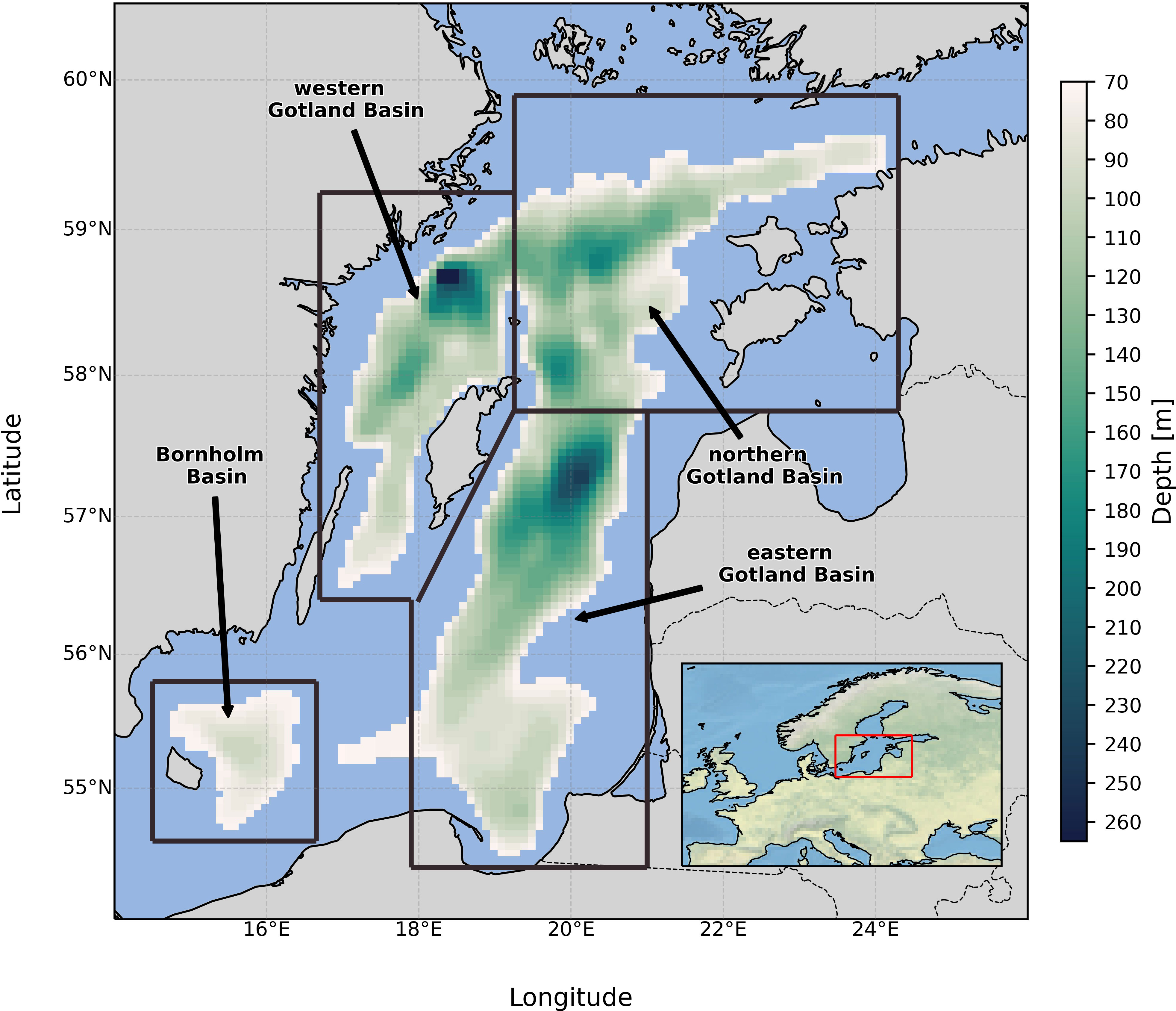
Figure 1 Location of the four studied sub-basins (boxes). Note that the upper boundary is located at 70 meters depth, so the depth counting starts at 70 meters.
2.3 Nutrient input scenarios
This study features three different nutrient input scenarios. The reference scenario is based on the simulation analyzed in Naumov et al. (2023). It employs HELCOM’s actual nutrient loads from 1948 to 2018 (Svendsen and Gustafsson, 2020). Data gaps were filled with linear interpolation. The BSAP scenario imposes constant nutrient loads based on the level of the Maximum Allowable Input (MAI) (HELCOM, 2021). The total input of P and N into the Baltic Sea at levels no more than the BSAP MAI should guarantee the Baltic Sea’s transition into a “good environmental status” (Borja et al., 2015). Since BSAP specifies only total loads without separating airborne and waterborne loads, the climatology seasonal cycle of the atmospheric nutrient input was applied. The halved BSAP MAI scenario (0.5 BSAP) assumes that the loads would be constant on the level of the half from the BSAP MAI (both waterborne and airborne input). The two reduction scenarios span the timeframe from 2019 to 2089 (71 years) and start from initial conditions taken from the last year of the reference scenario. Total nitrogen loads to the Baltic Sea under the BSAP scenario are set to 792.2 Kton/a (97% of the actual nitrogen loads averaged for the last ten years – 815.4 Kton/a). Under the 0.5 BSAP scenario, the total nitrogen loads equal 396.1 Kton/a (48% of the average actual loads for the last ten years). Total phosphorus loads under the BSAP and 0.5 BSAP scenarios equal 21.72 and 10.86 Kton/a, respectively. This constitutes 82 and 41% of the current total phosphorus loads – 26.33 Kton/a, respectively. So the BSAP goals have not been fully achieved yet, but the actual loads are very close to them. For more information, see Supplementary Figures 1, 2. In reference and nutrient reduction scenarios, we applied identical atmospheric forcing, namely CoastDat2 atmospheric fields from 1948 to 2018 (Geyer, 2014). Therefore, we neglect the impact of future climate change and natural variability, focusing only on the nutrient loads effect on the Baltic Sea’s eutrophication.
3 Results and discussion
3.1 Trends in O2 and H2S sources and sinks
Following the approach of Naumov et al. (2023), we aggregated all O2 and H2S budget terms into three categories based on their origin (physical or biological) and domain (water column or sediments): physical processes encompassing all oxygen fluxes with physical origin, mainly lateral and vertical advection (phy), oxygen fluxes with biological origin situated in the water column, e.g., remineralization of OM and zooplankton respiration (bio), and oxygen fluxes located in the sediments, e.g., remineralization of the sedimentary detritus (sed). Results are shown in Figure 2 (oxygen) and Supplementary Figure 3 (hydrogen sulfide). Figure 2 shows significant changes in the oxygen consumption pattern under both BSAP and 0.5 BSAP scenarios. Especially significant changes happened in the nGB, where oxygen consumption shifted back to the sediments at the end of the study period in both scenarios (with 0.5 BSAP amplifying the reported changes). The wGB demonstrates a similar pattern. However, it achieved sediment dominance in the consumption only under the 0.5 BSAP scenario. Under the BSAP scenario, a significant negative trend was only observed in sedimentary consumption. Elevated oxygen consumption in the sediments under BSAP and 0.5 BSAP scenarios, most visible in the nGB, can be interpreted as a positive sign indicating reoxygenation of the sediments. As was concluded by Naumov et al. (2023), less oxygen consumption in the sediments indicates the absence of oxygen, which means no electron acceptor available for the reactions. As sediments contact with oxygen again, the reduced material is getting oxidized promoting oxygen consumption in the sediments. This mechanism is more pronounced under the more rigorous 0.5 BSAP scenario. Noticeably, a significant positive trend in physical fluxes was observed under the 0.5 BSAP scenario, which is related to better ventilation due to the improved oxygen conditions in the neighboring nGB. Unlike nGB and wGB, BB and eGB are closer to the Baltic Sea’s entrance and therefore receive more oxygen via advection (Liblik et al., 2018; Naumov et al., 2023), do not demonstrate striking trends in consumption terms. The only significant trend in the BB is the positive trend in sedimentary consumption under the 0.5 BSAP scenario, indicating the best oxygen conditions among the studied subbasins. In the eGB, significant positive trends in the water column oxygen consumption were observed under both BSAP and 0.5 BSAP scenarios. It also points out the improvement because less consumption in the water column indicates less reduced material stored there. H2S sources and sinks (Supplementary Figure 3) also demonstrated substantial changes. By the end of the study period, the eGB came to the dynamic balance between H2S sources and sinks, indicating that H2S is not deposited. The same changes by the end of the period are observed even in the nGB under the 0.5 BSAP scenario. Under the BSAP scenario, a significant reduction in H2S production and consumption is observed in the nGB. However, it stabilizes in the 2070s. Despite that, advection to the upper layers in the nGB stops by the end of the study period in both scenarios. The wGB demonstrated the most noticeable difference between the BSAP and 0.5 BSAP scenarios. Under the BSAP scenario, wGB is still exporting H2S to the upper layer by the end of the study period, although to a much lower extent than in the beginning. Sedimentary production exhibits a significant negative trend but stabilizes in the 2070s, and water column consumption shows no trend under the BSAP scenario. Under the 0.5 BSAP scenario, both consumption and production of H2S converge to zero in the wGB, removing any export to the upper layers via advection.
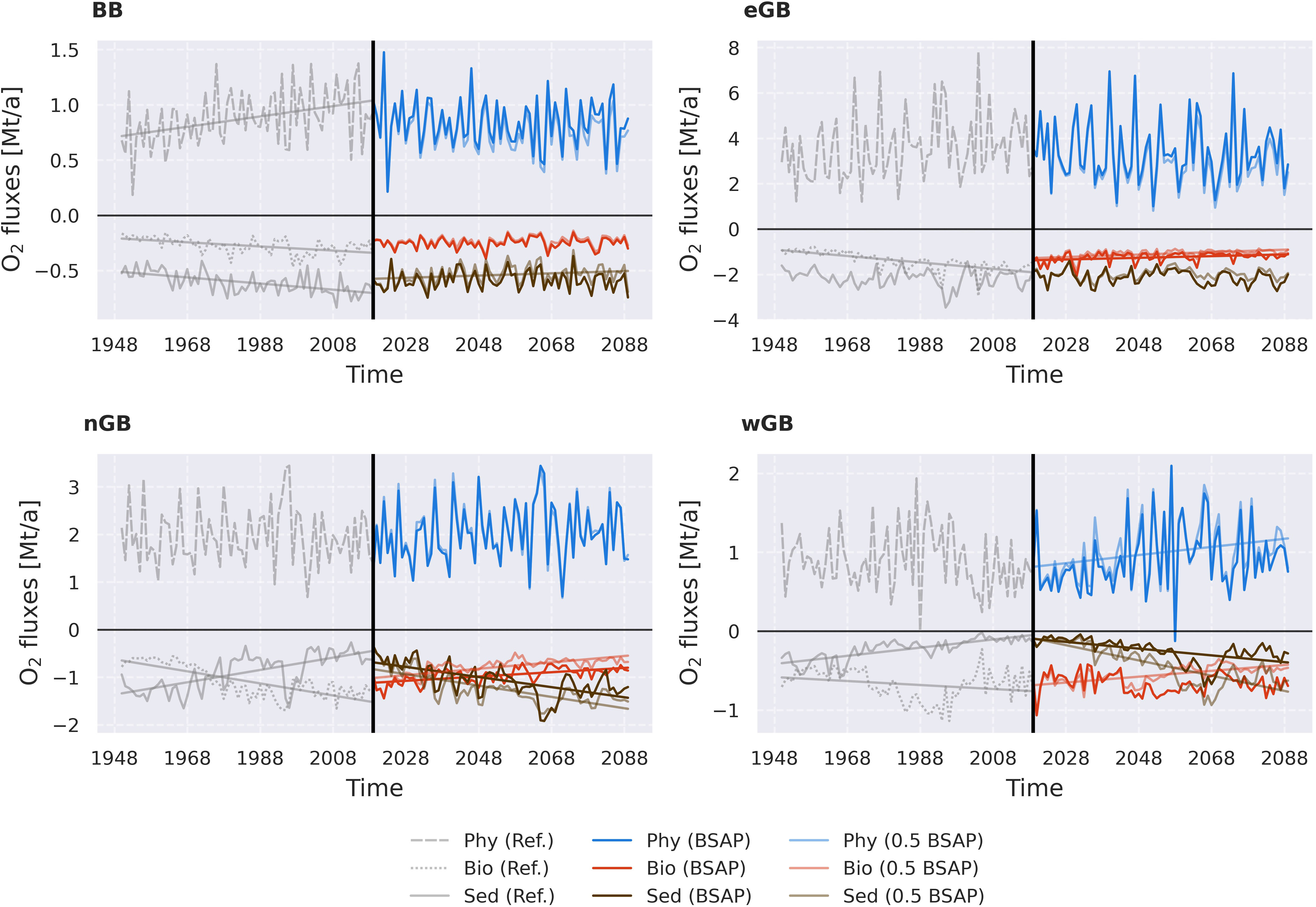
Figure 2 Temporal dynamics of the total annual oxygen fluxes by the three categories (physical fluxes – Phy (blue line), consumption in the water column – Bio (red line), and consumption in the sediments – Sed (dark brown line)). The categories are explained in more detail in the Section 3.1. For a list of processes comprising each category see Supplementary Table 1. Zero is marked by the horizontal black translucent line. Positive fluxes mean oxygen supply (only fluxes by the physical processes can be positive), and negative – oxygen consumption (by the water column and sedimentary processes). For negative oxygen fluxes (oxygen consumption), a negative linear trend means amplified oxygen consumption, and a positive – reduced consumption. The reversed logic is applicable to the positive fluxes (oxygen supply), where a positive trend means increasing supply and a negative – decreasing. Grey lines represent the reference scenario. Only significant linear trends (p< 0.05) are shown in the figure. Mt/a stands for 109 kg per year.
3.2 Budgets’ composition
To evaluate different sources and sinks’ contribution to the oxygen and hydrogen sulfide variability, we employed a linear regression framework proposed by Naumov et al. (2023). This linear model allows us to estimate the explained interannual variability by each group of processes. We used the same groups (phy, bio, and sed) as in the previous section. The results are shown in Figure 3. It can be seen that the general pattern is similar compared to the one by Naumov et al. (2023), which is advection dominance for oxygen in both considered scenarios. Another pattern for oxygen is less explained variability by the water column processes (especially in the BB and eGB) moving from the reference scenario to the 0.5 BSAP. This pattern complements the conclusions from the previous section, namely, the elevated variability of the sedimentary processes towards the end of the simulation. The composition of the processes contributing to the H2S budget is generally more complex (both regionally and in different scenarios). It points to the strong connection between H2S dynamics and nutrient forcing (see Supplementary Figure 4 for additional information). Overall, it can be stated that H2S dynamics is more affected by the nutrient loads reduction than oxygen dynamics, with some regional differences existing in both cases.
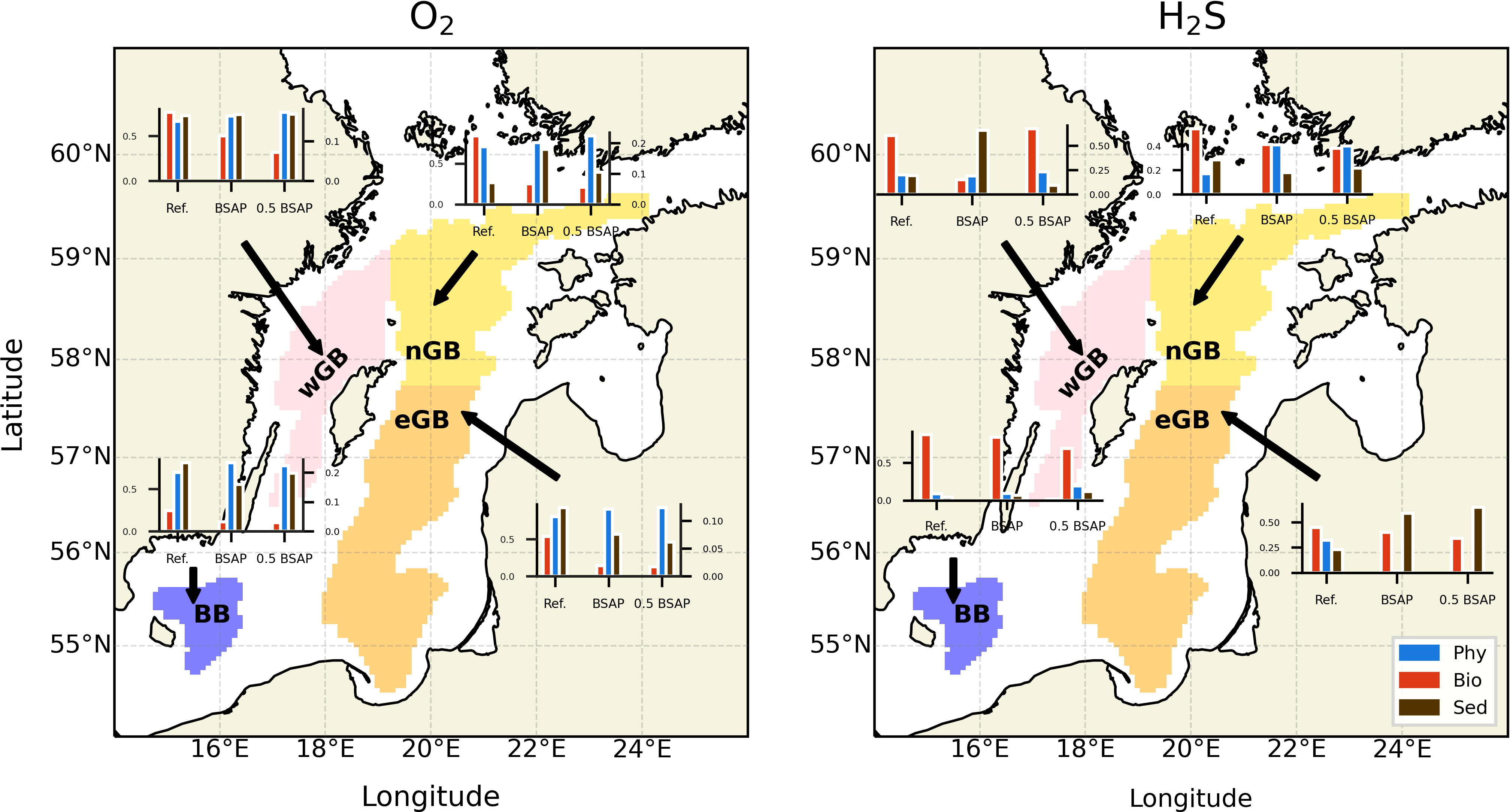
Figure 3 Maps showing different processes’ contributions to the O2 (left) and H2S (right) budgets in the water column of the four studying sub-basins. Processes are aggregated into the same three groups (phy, bio, and sed) as in Figure 2. More information about processes in each group can be found in Supplementary Tables 1 (oxygen) and 2 (hydrogen sulfide). In bar plots, the y-axis represents a fraction of the total variability explained by a certain group of processes, and the x-axis represents scenarios. Note that oxygen charts have two y-axes with different scales. The left and right axes represent the fraction of variability explained by the group phy and the groups bio as well as sed, respectively.
3.3 O2 and H2S dynamics induced by the nutrient forcing
Nutrient loads dynamics determine a significant fraction of oxygen variability in the Baltic Sea (Meier et al., 2019). Here, we quantify its contribution to the oxygen and hydrogen sulfide sources and sinks variability under the considered scenarios. We employed Empirical Orthogonal Functions (EOFs), based on eigenvectors and eigenvalues (Hannachi et al., 2007). It allows a decomposition of the complex multidimensional data into a set of orthogonal functions with a reduced number of dimensions by calculating eigenvalues and eigenvectors of the data’s correlation/covariation matrix and multiplying the latter with the original matrix. We applied such an EOF analysis to the matrixes of oxygen and hydrogen sulfide budget terms’ annual consumption/production anomalies during the reference period (1948-2018). Then we projected the resulting EOFs into future projections. Resulting EOFs are guaranteed to represent the same process during the reference period and future scenarios. The results are presented in Figure 4 (for oxygen) and Supplementary Figure 4 (for hydrogen sulfide). Based on the eigenvalues, the first three EOFs were considered significant for both elements (Panel A in Figure 4; Supplementary Figure 4). For O2, the first EOF explains around 60% of the total variability, the second EOF about 20%, and the third about 10%. For H2S, the eigenvalues converge quicker, with the first EOF already explaining 85% of the total variability and the last two EOFs around 5% each. The leading EOF in both O2 and H2S data can be attributed to the same process based on its loadings (Panel E in both figures). Both for O2 and H2S data, the leading EOF demonstrates a strong positive connection with anomalies of sedimentary detritus’ oxidation (either by oxygen or sulfate reduction). This means that when the score of the first EOF is positive (from the 1970s to the 2030s, according to Panel B in both figures), there is an intensified H2S production due to the mineralization of sedimentary detritus in the nGB. The same is true (but to a lesser extent) for the other regions of the Gotland Basin. At the same time, detritus is less mineralized by oxygen in the nGB and wGB but more in the eGB, indicating reduced material deposition in the nGB and wGB. The negative score of the first EOF, which is observed at the beginning of the reference period and after the 2030s, indicates the overall improvement of the oxygen conditions in the central Baltic Sea (no long-term deposition of the reduced material and oxidation of existing H2S, especially in the remote basins). This allowed us to attribute the leading EOF to the nutrient forcing. The last two EOFs were attributed to the inflow activity and natural variability. They do not exhibit any significant difference between the reference period and the future projections (for both BSAP and 0.5 BSAP scenarios). The first EOFs for BSAP and 0.5 BSAP are highly correlated (>0.9), which suggests that there are no significant differences in how the nutrient load reduction affects the marine system for the BSAP and more rigorous 0.5 BSAP scenarios; however, the first EOF for 0.5 BSAP scenario shows a more negative score compared to the first EOF of the BSAP scenario, which means the more resilient state and more improvement.
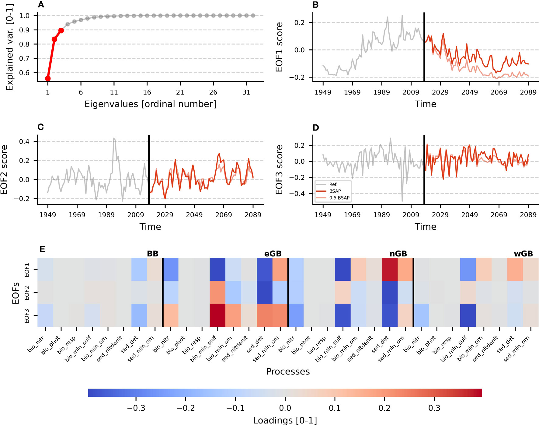
Figure 4 EOF decomposition of the spatial-temporal matrix of oxygen consumption terms aggregated into specific groups. Group names [x-axis labels in E)] should be read as follows:<domain>_<name of processes>. There are two domains: bio – water column, and sed – sediments; and six processes: nitr/nitdenit – nitrification, phot – photosynthesis, resp – respiration of biota, min_sulf – nineralization of sulfur, min_om – mineralization of organic matter, det – mineralization of detritus only. To get more information about individual processes in the group, see Supplementary Table 1. (A) Shows the fraction of variability explained by all calculated EOFs. Only the first three EOFs were considered significant and used later in the analysis [colored red in (A)]. (B–D) Depict the temporal variability of the first three EOFs correspondingly. Here, the black vertical line demarcates the reference scenario (grey curve) and BSAP, 0.5 BSAP scenarios (vivid and translucent red lines, correspondingly). (E) Demonstrates the loadings of the first three EOFs. Loadings vary from minus one to one and show the direction and magnitude of the connection between an EOF and a variable. Black lines highlight the spatial structure of the matrix by separating the sub-basins.
3.4 Discussion
Our results suggest that oxygen conditions in the central Baltic Sea will substantially improve both under BSAP and 0.5 BSAP scenarios, especially in the remote nGB and wGB, which, however, did not significantly diminish the hypoxic area, only the anoxic area significantly shrank at the end of the study period (see Supplementary Figure 5), which is related to the significant oxygen debt in the deep central Baltic Sea (Rolff et al., 2022). However, our study uses atmospheric forcing from 1948-2018, which completely ignores possible changes, such as changes in stratification and internal nutrient cycle (Meier et al., 2011; Hordoir and Meier, 2012), that could worsen the results to some extent, but, based on the results by Saraiva et al. (2019); Meier et al. (2021) and Bartosova et al. (2019), the effect of nutrient load reduction policy should dominate climate change impacts, at least in the near future. Elevated halocline strength observed in the model (Naumov et al., 2023) also worsens oxygen conditions in the deep sea, which could mimic the negative effects in the real system related to climate change. Still, the dynamics of cyanobacteria blooms might be underestimated in the model since their blooms may get amplified by climate change. Since significant positive trends in nitrates were observed everywhere across the Gotland Basin (see Supplementary Figures 6–9), it could potentially lead to a serious deterioration in case of a sudden short-time anoxia and release of the sedimentary phosphorus (Mort et al., 2010). Another possible shortcoming of the study is related to the difficulties in validating the sources and sinks of O2 and H2S due to the lack of proper observational data (long-term monitoring at the specific station in the deep Baltic Sea). Only studies by Schneider et al. (2010) and Gustafsson and Stigebrandt (2007) reconstructed the oxygen sources and sinks based on observational data. Unfortunately, their results cannot be qualitatively compared to our model findings due to the different spatiotemporal scales and different formulations of processes in the model. Still, they exhibit similar patterns (elevated oxygen consumption by nitrification after more oxygen enters the system, for example).
4 Conclusions
1. The central Baltic Sea under the MAIs of the BSAP and the halved BSAP showed an improvement and transition to a more oxic state after 2018 within the simulated 71 years. However, the hypoxic area did not reduce dramatically in both scenarios, pointing out the high oxygen debt in the deep central Baltic Sea.
2. Positive changes were observed in all regions of the Gotland Basin, especially in the remote northern and western Gotland basins. In the nGB, a shift from consumption in the water column to consumption in the sediments was observed in both BSAP and 0.5 BSAP. In the wGB, the same changes were observed under 0.5 BSAP. Positive trends in the water column oxygen consumption are mostly explained by the reduced oxidation of hydrogen sulfide and nitrification towards the end of the simulation (the year 2089). In the sediments, the increased consumption is mostly attributed to the elevated oxidation of organic matter towards the end of the simulation. Faster improvement in the remote basins was attributed to the positive feedback related to the reduction of H2S concentration in eGB and, therefore, its less advection to the nGB and wGB. Elevated oxygen concentrations in the eGB could also lead to more effective ventilation of the remote basins by inflowing oxygen due to reduced consumption on the way to the remote basins.
3. The general trend to the less explained variance by water column oxygen consumption and more by the sedimentary oxygen consumption was found across all studied subbasins. Physical fluxes (mainly advection) explain most oxygen variability in all scenarios. Hydrogen sulfide dynamics was found to be more region dependent and influenced by the different nutrient input scenarios.
4. Three EOFs were identified as patterns governing the dynamics of oxygen and hydrogen sulfide in the reference scenario. For oxygen budget terms, the first EOF explained approx. 60% of the variability, the second – approx. 20%, and the third – approx. 10%. For the hydrogen sulfide dynamics, the first EOF explained more than 80% of the variability, and all three EOFs together explained more than 95%. The last two EOFs were attributed to the inflows’ activity and the natural variability, and the first EOF – to the change in the nutrient forcing with positive (deposition of reduced material and organic matter, deoxygenation) and negative (oxidation of the reduced material, oxygenation) phases. The first EOF went into the constant negative phase (no deposition of reduced material and oxidation of already existing one) in the 2050s (O2, BSAP), the 2030s (O2, 0.5 BSAP), and the 2030s (H2S, both BSAP and 0.5 BSAP), indicating resilient transformation to the oxic regime.
5. According to our model study, it is possible for the Baltic Sea to return to its initial state (the year 1948) within 71 years under the 0.5 BSAP scenario (see Figures 2, 4). Under the BSAP scenario, the Baltic Sea state comes close to the initial state but did not reach it within the simulation time.
Data availability statement
Baltic Sea Action Plan Maximum allowable input nutrient loads (2021 update) can be found within the following document: https://helcom.fi/wp-content/uploads/2021/10/Baltic-Sea-Action-Plan-2021-update.pdf. The generated model data needed for reproducing the analysis can be found on the IOW server (http://doi.io-warnemuende.de/10.12754/data-2023-0009).
Author contributions
LN prepared the nutrient input datasets with the help of TN. LN performed the simulations and analyzed the data. LN and HEMM designed the research. HEMM supervised the work. All authors contributed to the article and approved the submitted version.
Funding
We thank the Open Access Fund of Leibniz Association for funding the publication of this article.
Acknowledgments
The research presented in this study is part of the Baltic Earth program (Earth System Science for the Baltic Sea region, see http://www.baltic.earth). The model simulations were performed on the North German Supercomputing Alliance (HLRN) computers. In addition, we thank two reviewers for their helpful comments that improved the manuscript’s quality.
Conflict of interest
The authors declare that the research was conducted in the absence of any commercial or financial relationships that could be construed as a potential conflict of interest.
Publisher’s note
All claims expressed in this article are solely those of the authors and do not necessarily represent those of their affiliated organizations, or those of the publisher, the editors and the reviewers. Any product that may be evaluated in this article, or claim that may be made by its manufacturer, is not guaranteed or endorsed by the publisher.
Supplementary material
The Supplementary Material for this article can be found online at: https://www.frontiersin.org/articles/10.3389/fmars.2023.1233324/full#supplementary-material
References
Almroth-Rosell E., Wåhlström I., Hansson M., Väli G., Eilola K., Andersson P., et al. (2021). A regime shift toward a more anoxic environment in a Eutrophic sea in Northern Europe. Front. Mar. Sci. 8. doi: 10.3389/fmars.2021.799936
Ator S. W., Blomquist J. D., Webber J. S., Chanat J. G. (2020). Factors driving nutrient trends in streams of the Chesapeake Bay watershed. J. Environ. Qual. 49, 812–834. doi: 10.1002/jeq2.20101
Backer H., Leppänen J.-M., Brusendorff A. C., Forsius K., Stankiewicz M., Mehtonen J., et al. (2010). HELCOM Baltic Sea Action Plan – A regional programme of measures for the marine environment based on the Ecosystem Approach. Mar. pollut. Bull. 60, 642–649. doi: 10.1016/j.marpolbul.2009.11.016
Bartosova A., Capell R., Olesen J. E., Jabloun M., Refsgaard J. C., Donnelly C., et al. (2019). Future socioeconomic conditions may have a larger impact than climate change on nutrient loads to the Baltic Sea. Ambio 48, 1325–1336. doi: 10.1007/s13280-019-01243-5
Borja A., Elliott M., Andersen J. H., Cardoso A. C., Carstensen J., Ferreira J. G., et al. (2015). Report on potential Definition of Good Environmental Status. Deliverable 6.2. (DEVOTES Project). 62pp. Available at: https://mcc.jrc.ec.europa.eu/documents/201502120842.pdf
Breitburg D., Levin L., Oschlies A., Grégoire M., Chavez F., Conley D., et al. (2018). Declining oxygen in the global ocean and coastal waters. Sci. (New York N.Y.) 359, 7240. doi: 10.1126/science.aam7240
Conley D. J., Björck S., Bonsdorff E., Carstensen J., Destouni G., Gustafsson B. G., et al. (2009). Hypoxia-related processes in the Baltic Sea. Environ. Sci. Technol. 43, 3412–3420. doi: 10.1021/es802762a
Diaz R. J., Rosenberg R. (2008). Spreading dead zones and consequences for marine ecosystems. Science 321, 926–929. doi: 10.1126/science.1156401
Fennel K., Testa J. M. (2019). Biogeochemical controls on coastal hypoxia. Annu. Rev. Mar. Sci. 11, 105–130. doi: 10.1146/annurev-marine-010318-095138
Friedland R., Neumann T., Schernewski G. (2012). Climate change and the Baltic Sea action plan: Model simulations on the future of the western Baltic Sea. J. Mar. Syst. 105–108, 175–186. doi: 10.1016/j.jmarsys.2012.08.002
Geyer B. (2014). High-resolution atmospheric reconstruction for Europe 1948–2012: coastDat2. Earth Sys. Sci. Data 6, 147–164. doi: 10.5194/essd-6-147-2014
Griffies S. M. (2012). Elements of the modular ocean model. GFDL ocean group technical report no. 7 (Princeton, NJ, USA: NOAA/Geophysical Fluid Dynamics Laboratory), 632.
Gustafsson B. G., Schenk F., Blenckner T., Eilola K., Meier H. E. M., Müller-Karulis B., et al. (2012). Reconstructing the development of Baltic Sea eutrophication 1850–2006. AMBIO 41, 534–548. doi: 10.1007/s13280-012-0318-x
Gustafsson B. G., Stigebrandt A. (2007). Dynamics of nutrients and oxygen/hydrogen sulfide in the Baltic Sea deep water. J. Geophys. Res.: Biogeosci. 112, G02023. doi: 10.1029/2006JG000304
Hannachi A., Jolliffe I. T., Stephenson D. B. (2007). Empirical orthogonal functions and related techniques in atmospheric science: A review. Int. J. Climatol. 27, 1119–1152. doi: 10.1002/joc.1499
Hansson M., Viktorsson L. (2020). Oxygen Survey in the Baltic Sea 2020 - Extent of Anoxia and Hypoxia 1960-2020. Report Oceanography no. 70 (Göteborg: Swedish Meteorological and Hydrological Institute).
Heathwaite A. L., Johnes P. J., Peters N. E. (1996). Trends in nutrients. Hydrol. Processes 10, 263–293. doi: 10.1002/(SICI)1099-1085(199602)10:2<263::AID-HYP441>3.0.CO;2-K
HELCOM (2007). The HELCOM Baltic Sea Action Plan (Helsinki: Helsinki Commission). Available at: www.helcom.fi.
Hordoir R., Meier H. E. M. (2012). Effect of climate change on the thermal stratification of the baltic sea: a sensitivity experiment. Clim Dyn 38, 1703–1713. doi: 10.1007/s00382-011-1036-y
Knuuttila S., Räike A., Ekholm P., Kondratyev S. (2017). Nutrient inputs into the Gulf of Finland: Trends and water protection targets. J. Mar. Syst. 171, 54–64. doi: 10.1016/j.jmarsys.2016.09.008
Kõuts M., Maljutenko I., Elken J., Liu Y., Hansson M., Viktorsson L., et al. (2021). Recent regime of persistent hypoxia in the Baltic Sea. Environ. Res. Commun. 3, 075004. doi: 10.1088/2515-7620/ac0cc4
Krapf K., Naumann M., Dutheil C., Meier H. E. M. (2022). Investigating hypoxic and euxinic area changes based on various datasets from the Baltic Sea. Front. Mar. Sci. 9, 823476doi: 10.3389/fmars.2022.823476
Kuznetsov I., Neumann T. (2013). Simulation of carbon dynamics in the Baltic Sea with a 3D model. J. Mar. Syst. 111–112, 167–174. doi: 10.1016/j.jmarsys.2012.10.011
Large W. G., McWilliams J. C., Doney S. C. (1994). Oceanic vertical mixing: a review and a model with a nonlocal boundary layer parameterization. Rev. Geophys. 32, 363–403. doi: 10.1029/94RG01872
Larsson U., Elmgren R., Wulff F. (1985). Eutrophication and the Baltic Sea: causes and consequences. Ambio 14, 1–6.
Lenz C., Jilbert T., Conley D. J., Slomp C. P. (2015). Hypoxia-driven variations in iron and manganese shuttling in the Baltic Sea over the past 8 kyr. Geochem. Geophys. Geosys. 16, 3754–3766. doi: 10.1002/2015GC005960
Leppäranta M., Myrberg K. (2009). Physical Oceanography of the Baltic Sea (Berlin, Heidelberg: Springer). doi: 10.1007/978-3-540-79703-6
Liblik T., Naumann M., Alenius P., Hansson M., Lips U., Nausch G., et al. (2018)Propagation of impact of the recent major Baltic inflows from the Eastern Gotland basin to the gulf of Finland (Accessed February 15, 2023).
Meier H. E. M., Andersson H. C., Eilola K., Gustafsson B. G., Kuznetsov I., Müller-Karulis B., et al. (2011). Hypoxia in future climates: A model ensemble study for the Baltic Sea. Geophys. Res. Lett. 38. doi: 10.1029/2011GL049929
Meier H. E. M., Dieterich C., Gröger M. (2021). Natural variability is a large source of uncertainty in future projections of hypoxia in the Baltic Sea. Commun. Earth Environ. 2, 1–13. doi: 10.1038/s43247-021-00115-9
Meier H. E. M., Dieterich C., Gröger M., Dutheil C., Börgel F., Safonova K., et al. (2022). Oceanographic regional climate projections for the Baltic Sea until 2100. Earth Sys. Dynamics 13, 159–199. doi: 10.5194/esd-13-159-2022
Meier H. E. M., Eilola K., Almroth-Rosell E., Schimanke S., Kniebusch M., Höglund A., et al. (2019). Disentangling the impact of nutrient load and climate changes on Baltic Sea hypoxia and eutrophication since 1850. Clim Dyn 53, 1145–1166. doi: 10.1007/s00382-018-4296-y
Meier H. E. M., Väli G., Naumann M., Eilola K., Frauen C. (2018). Recently accelerated oxygen consumption rates amplify deoxygenation in the Baltic Sea. J. Geophys. Res.: Oceans 123, 3227–3240. doi: 10.1029/2017JC013686
Mort H. P., Slomp C. P., Gustafsson B. G., Andersen T. J. (2010). Phosphorus recycling and burial in Baltic Sea sediments with contrasting redox conditions. Geochimica Cosmochimica Acta 74, 1350–1362. doi: 10.1016/j.gca.2009.11.016
Naumov L., Neumann T., Radtke H., Meier H. E. M. (2023). Limited ventilation of the central Baltic Sea due to elevated oxygen consumption. Front. Mar. Sci. doi: 3389/fmars.2023.1175643
Neumann T. (2010). Climate-change effects on the Baltic Sea ecosystem: A model study. J. Mar. Syst. 81, 213–224. doi: 10.1016/j.jmarsys.2009.12.001
Neumann T., Eilola K., Gustafsson B., Müller-Karulis B., Kuznetsov I., Meier H. E. M., et al. (2012). Extremes of temperature, oxygen and blooms in the Baltic Sea in a changing climate. AMBIO 41, 574–585. doi: 10.1007/s13280-012-0321-2
Neumann T., Fennel W., Kremp C. (2002). Experimental simulations with an ecosystem model of the Baltic Sea: A nutrient load reduction experiment: NUTRIENT LOAD REDUCTION EXPERIMENT. Global Biogeochem. Cycles 16, 7-1-7–7-119. doi: 10.1029/2001GB001450
Neumann T., Koponen S., Attila J., Brockmann C., Kallio K., Kervinen M., et al. (2021). Optical model for the Baltic Sea with an explicit CDOM state variable: a case study with Model ERGOM (version 1.2). Geosci. Model. Dev. 14, 5049–5062. doi: 10.5194/gmd-14-5049-2021
Neumann T., Radtke H., Cahill B., Schmidt M., Rehder G. (2022). Non-Redfieldian carbon model for the Baltic Sea (ERGOM version 1.2) – implementation and budget estimates. Geosci. Model. Dev. 15, 8473–8540. doi: 10.5194/gmd-15-8473-2022
Radtke H., Lipka M., Bunke D., Morys C., Woelfel J., Cahill B., et al. (2019). Ecological Regional Ocean Model with vertically resolved sediments (ERGOM SED 1.0): coupling benthic and pelagic biogeochemistry of the south-western Baltic Sea. Geosci. Model. Dev. 12, 275–320. doi: 10.5194/gmd-12-275-2019
Rolff C., Walve J., Larsson U., Elmgren R. (2022). How oxygen deficiency in the Baltic Sea proper has spread and worsened: The role of ammonium and hydrogen sulphide. Ambio 51, 2308–2324. doi: 10.1007/s13280-022-01738-8
Rydin E., Kumblad L., Wulffe F., Larsson JP. (2017). Remediation of a Eutrophic Bay in the Baltic Sea. Environ. Sci. Technol. 51, 4559–4566. doi: 10.1021/acs.est.6b06187
Saraiva S., Meier H. E. M., Andersson H., Höglund A., Dieterich C., Gröger M., et al. (2019). Uncertainties in projections of the Baltic Sea ecosystem driven by an ensemble of global climate models. Front. Earth Sci. 6. doi: 10.3389/feart.2018.00244
Savchuk O. P. (2018)Large-scale nutrient dynamics in the Baltic Sea 1970–2016 (Accessed February 15, 2023).
Schneider B., Nausch G., Pohl C. (2010). Mineralization of organic matter and nitrogen transformations in the Gotland Sea deep water. Mar. Chem. 119, 153–161. doi: 10.1016/j.marchem.2010.02.004
Stoicescu S.-T., Lips U., Liblik T. (2019)Assessment of eutrophication status based on sub-surface oxygen conditions in the gulf of Finland (Baltic Sea) (Accessed May 22, 2023).
Svendsen L. M., Gustafsson B. (2020) Waterborne nitrogen and phosphorus inputs and water flow to the Baltic Sea 1995—2018. Available at: https://helcom.fi/baltic-sea-trends/environment-fact-sheets/eutrophication/ (Accessed May 22, 2023).
Uurasjärvi E., Pääkkönen M., Setälä O., Koistinen A., Lehtiniemi M. (2021). Microplastics accumulate to thin layers in the stratified Baltic Sea. Environ. pollut. 268, 115700. doi: 10.1016/j.envpol.2020.115700
Vahtera E., Conley D. J., Gustafsson B. G., Kuosa H., Pitkänen H., Savchuk O. P., et al. (2007). Internal ecosystem feedbacks enhance nitrogen-fixing cyanobacteria blooms and complicate management in the Baltic Sea. AMBIO 36, 186–194. doi: 10.1579/00447447
Väli G., Meier H. E. M., Elken J. (2013). Simulated halocline variability in the Baltic Sea and its impact on hypoxia during 1961-2007: SIMULATED HALOCLINE VARIABILITY IN THE BALTIC SEA. J. Geophys. Res. Oceans 118, 6982–7000. doi: 10.1002/2013JC009192
Voss M., Dippner J. W., Humborg C., Hürdler J., Korth F., Neumann T., et al. (2011). History and scenarios of future development of Baltic Sea eutrophication. Estuarine Coast. Shelf Sci. 92, 307–322. doi: 10.1016/j.ecss.2010.12.037
Whitney M. M. (2022). Observed and projected global warming pressure on coastal hypoxia. Biogeosciences 19, 4479–4497. doi: 10.5194/bg-19-4479-2022
Keywords: Baltic Sea, O2 and H2S sources and sinks, Baltic Sea Action Plan, nutrient reduction, modeling
Citation: Naumov L, Meier HEM and Neumann T (2023) Dynamics of oxygen sources and sinks in the Baltic Sea under different nutrient inputs. Front. Mar. Sci. 10:1233324. doi: 10.3389/fmars.2023.1233324
Received: 01 June 2023; Accepted: 21 July 2023;
Published: 11 August 2023.
Edited by:
Elinor Andrén, Södertörn University, SwedenReviewed by:
Tarang Khangaonkar, Pacific Northwest National Laboratory (DOE), United StatesAdolf Konrad Stips, European Commission, Italy
Copyright © 2023 Naumov, Meier and Neumann. This is an open-access article distributed under the terms of the Creative Commons Attribution License (CC BY). The use, distribution or reproduction in other forums is permitted, provided the original author(s) and the copyright owner(s) are credited and that the original publication in this journal is cited, in accordance with accepted academic practice. No use, distribution or reproduction is permitted which does not comply with these terms.
*Correspondence: Lev Naumov, bGV2Lm5hdW1vdkBpby13YXJuZW11ZW5kZS5kZQ==