Bed level changes in the surf zone during post-storm beach recovery

The study of post-storm beach recovery is important for economic development and the protection of life in coastal areas. In this study, field observations were conducted for 21 days in the surf zone of Dongdao Beach, Hailing Island, China, after tropical storm “Cempaka”. Data on depth, wave, Eulerian velocity, sediment, three-dimensional topography of the beach, and high-frequency variations in bed-level elevation were collected. The results showed that the beach experienced medium- to low- to medium-energy waves during field observations and covered two complete astronomical tide cycles. Contrary to the effect of wave energy conditions on beaches under normal wave conditions, a higher wave energy during beach recovery can promote silting and accelerate beach recovery. Tidal water level is an important factor affecting beach restoration, and a smaller tidal range is conducive to beach accretion. In a mixed semidiurnal tide, beach erosion and accretion occurred in the “highest tide” and “sub-highest tide” tidal cycles, respectively, and the combined effect of the two affected the change in the bed level in a mixed semidiurnal tide. After the storm, the hydrodynamic forcing mechanism and self-organization process of the sand bar jointly drove the formation of the topography of the bar channel in the surf zone. After the storm stopped, the spectral energy in free surface elevation was mainly distributed in the very low frequency and decayed rapidly at the infragravity band. The very low-frequency pulsation of the surf zone during recovery is a prominent feature of bed-level elevation, depth, and velocity. This study provides a good case for the study of hydrodynamic and bed level changes in the post-storm surf zone, as well as a reference for future studies of the intrinsic mechanisms post-storm beach recovery processes around the world.

1 Introduction

Beaches are a highly dynamic and active morphological system that connects land and ocean and is an area of strong land–sea interaction. Beaches, as geomorphological units of coastal sedimentary dynamics, maintain long-term equilibrium, but this equilibrium is disrupted after extreme events such as storms (Gervais et al., 2012). Beaches are natural barriers that protect coastal areas from extreme storm surges and sea level rise (Stive et al., 2013; Van Rijn, 2009; Van Rijn, 2011; Van Slobbe et al., 2013). During a storm, the strong wind and dramatic pressure changes can cause a storm surge on the sea surface that is different from normal hydrological conditions. This can lead to a rapid increase in water levels and accompanying intense waves, which can result in major changes to beach topography and the redistribution of sediment over a short period of time (Coco et al., 2014). Typhoons are among the deadliest nearshore natural disasters that not only exacerbate shoreline and dune erosion and cause damage to coastal infrastructure but also potentially result in considerable loss of life and long-term economic problems (Sallenger et al., 2006; Roelvink et al., 2009; Sherman et al., 2013). Severe destruction caused by typhoons is an important topic in coastal research (Regnauld et al., 2004; Qi et al., 2010; Brenner et al., 2018). Conducting field observations during storms is both difficult and dangerous. Nevertheless, some researchers have performed simultaneous measurements of hydrodynamics and bed level changes during storms (Zeng et al., 2020; Hu et al., 2022).

The surf zone is the channel for the exchange of sediments between the beach and nearshore. The change in the beach bed level is a hot topic in the research on the range of the surf zone. Most of the research on bed level changes is conducted under normal wave conditions (Kroon and Masselink, 2002; Masselink et al., 2008; Biausque and Senechal, 2019), and only a few researchers have performed high-frequency measurements of bed-level elevation (BLE) within tidal cycles (Saulter et al., 2003; Puleo et al., 2014; Pang et al., 2021). Puleo et al. (2014) used a new conductivity concentration profiler on a dissipative beach to quantify the bed level changes throughout the tidal cycle. They found that only a few “large” events may ultimately result in net bed level change within the tidal cycles and bed elevation time series were most energetic in the low-frequency band. Pang et al. (2021) used acoustic Doppler velocimeters on a meso–macro tidal beach to detect the characteristics of bed level changes at intratidal and tidal cycle scales. They found that the variations in the bed level were more prominent during neap to middle tides than during middle to spring tides, and the bed level displayed an increase during floods and decrease during ebb tides in the entire tidal cycle.

The hydrodynamic and bed level changes within the surf zone during post-storm beach recovery are complex, and much work has been conducted on beach restoration processes through descriptions of short- or long-term changes in beach profiles, shoreline morphology, and sediment characteristics (Qi et al., 2010; Ciavola and Coco, 2017; Ge et al., 2017; Dodet et al., 2019). Depending on the hydrodynamic and sediment budget conditions within the surf zone, the recovery period may vary from days to decades (Lee et al., 1998). Morton et al. (1994) proposed the classical theory for beach recovery stages, which indicates that short-term beach recovery (from several weeks to 1 year) typically begins immediately after a storm and is characterized by foreshore steepening, berm reconstruction, and landward migration of the innermost bar. After a storm, during relatively low-wave-power conditions, beaches favor accretion, which is a much slower process than erosion (Thom and Hall, 1991). Yu et al. (2013) investigated the beach profiles and sediment characteristics under two different wave energy conditions after a storm and found that high-energy beaches showed faster natural recovery after a storm, whereas low-energy beaches showed longer natural recovery periods.

Although much attention has been paid to beach bed level changes, few researchers have accurately measured bed level change during beach recovery after storms. In addition, in most previous studies, data of bed level change were obtained at low tides (when the beach surface was exposed to air) using the inserted rods, (Masselink et al., 1997; Agredano et al., 2019) which has a low sampling frequency, has high measurement error, and does not measure the process of bed level change underwater. Therefore, in this study, a 21-day field experiment was conducted from 08/08/2021 to 30/08/2021, in the surf zone of the Dongdao Beach of Hailing Island, China, after storm Cempaka, using five precision autonomous hydroacoustic altimeters (Echologger AA400, PAA) to accurately measure high-frequency bed level changes during beach recovery. This work presents the field findings of the high-frequency changes in BLE and hydrodynamics in the surf zone after the storm, with main aims (1) to explore the characteristics of bed level changes in the surf zone after the storm and (2) to study the influencing factors and their interactions during beach recovery. This study provides a good case for the study of hydrodynamic and bed level changes in the post-storm surf zone, as well as a reference for future studies on the intrinsic mechanisms of beach recovery processes after storms around the world.

2 Data and methods

2.1 Study area and storm

China is among the countries most frequently affected by tropical cyclones in the world, with more than 87% of tropical cyclone landfalls in southern China occurring in Guangdong and Hainan provinces (Zeng et al., 2020). The study area is located on Dongdao Beach on the southeastern side of Hailing Island, Yangjiang City, Guangdong Province, China, facing the South China Sea to the south and is an important tourist attraction in South China (Figure 1A). Dongdao Beach is an arc-shaped coast, approximately 4 km long and 80–100 m wide. There is a natural headland with a length of approximately 550 m on the east side of the beach. The eastern shoreline of the beach is perpendicular to the north direction and is connected to the headland, and the western shoreline and the north direction form an angle of approximately 60° clockwise (Figure 1C).

FIGURE 1

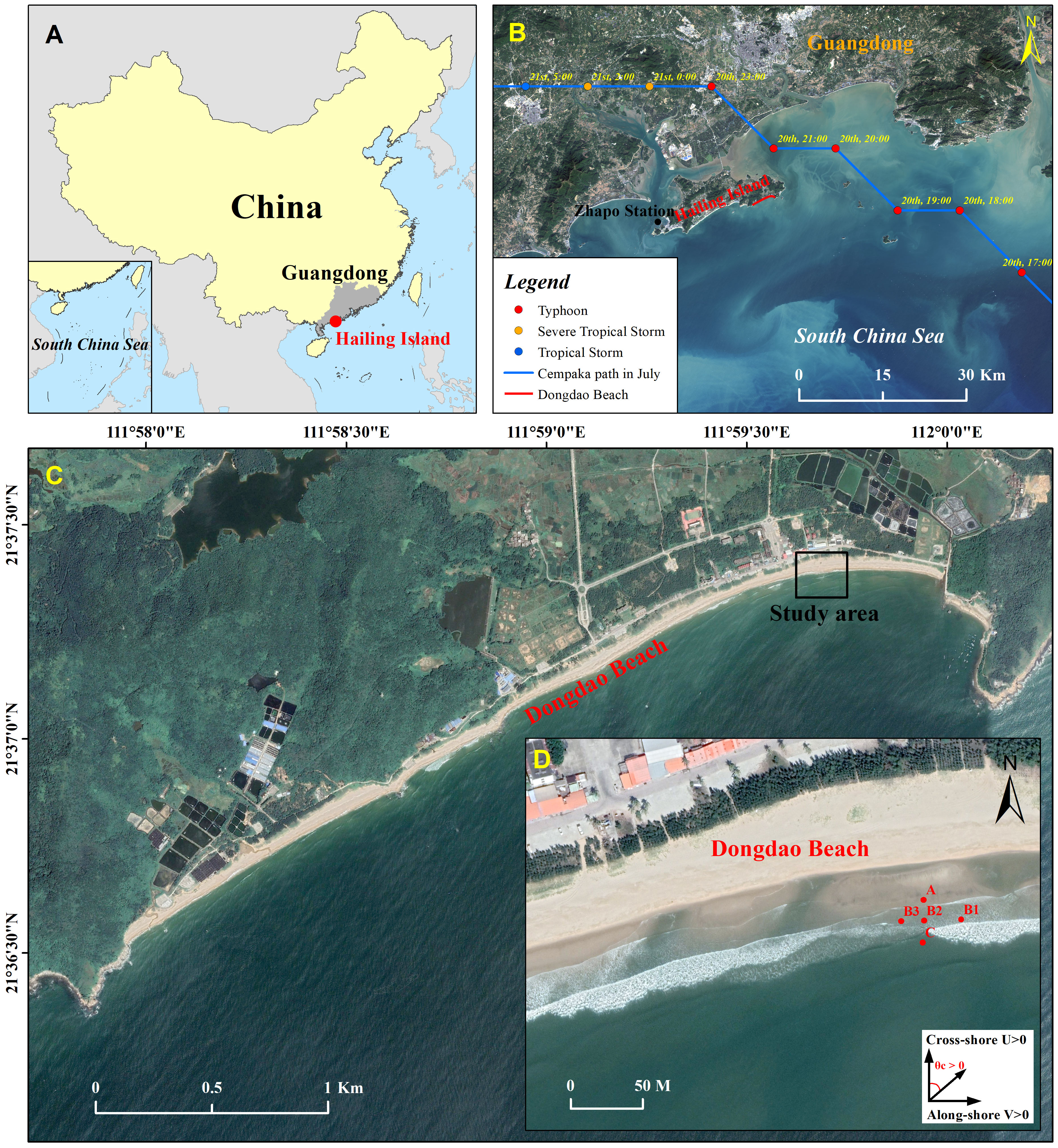
Figure 1 (A) Location of Hailing Island in China. (B) Satellite image of Hailing Island; the solid blue line shows the path of “Cempaka” in July 2021, the colored dots on the path indicate the storm center at different times, and the red solid line indicates the location of Dongdao Beach. (C) Satellite image of Dongdao Beach; the black rectangular box represents the study area. (D) Satellite image map of the study area, which shows the distribution of measurement sites.

Dongdao Beach is an open, high-energy beach with Casuarina equisetifolia planted along the shoreline for wind and sand stabilization. According to long-term tide level data from Zhapo Ocean Station (21°35′N, 111°50′E) in Hailing Island, the tide type is a mixed semidiurnal tide with a multiyear mean tidal difference of 1.54 m, a maximum tidal difference of 3.76 m, and a mean spring tidal difference of 2.08 m. The study area was dominated by a mixture of wind waves and swells. The wave direction was south, the occurrence frequency of waves with a height above 1.0 m was 35.8%, and the wave period was 2 s–6 s. The sediment is mainly composed of fine to medium quartz sand. According to the classical theory of beach morphodynamic classification (Wright and Short, 1984; Masselink and Short, 1993; Li, 2016), the studied beach is barred-type beach in the intermediate state characterized by a dimensionless fall velocity (Ω) of 4.4 and a relative tidal range (RTR) of 1.7. Submerged linear sandbars existed along shore, and the beach was able to recover quickly.

At 14:00 on 18/07/2021, the National Meteorological Centre (NMC) reported that tropical storm “Cempaka” formed over the South China Sea approximately 145 km southeast of Yangjiang City. At 23:00 on July 19, it became a typhoon at 84 km from Hailing Island, which carried maximum sustained winds of 33 m/s. Hailing Island was only 10 km from the center of the typhoon (Figure 1B). The observation area was located on the east side of Dongdao Beach, with S-direction waves incident vertically on the beach. This area was closer to the storm path compared with other areas of the beach. Affected by the storm, the observation area experienced strong erosion (Figure 2A and the bar-channel topography appeared before the storm and disappeared after the typhoon).

FIGURE 2

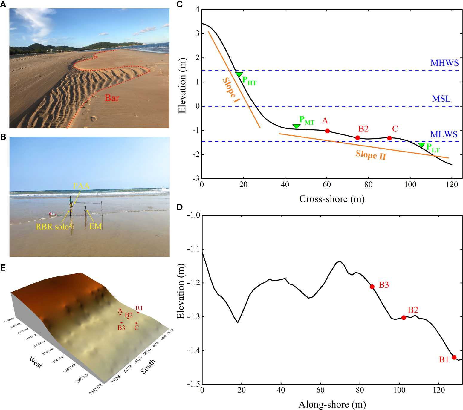
Figure 2 (A) On 15/07/2021, the topography of the bar channel was photographed before the typhoon in the study area, which disappeared after the storm. (B) Instrument deployment at site B2. (C) Cross-shore profile of the beach at the measurement site; red dots represent cross-shore measurement sites, green triangles represent three sediment sampling points, blue dotted lines represent mean high water springs (MHWS), mean sea level (MSL), and mean low water springs (MLWS), and yellow solid lines represent different slopes. The profiles in (C, D) were measured on August 22. (D) Along-shore profile of the beach at the measurement site; red dots represent along-shore measurement sites. (E) Three-dimensional topography of the surf zone on 22/08/2021, showing the three-dimensional distribution of measurement sites.

2.2 Instrument deployment

In the surf zone of study area, five measurement sites in three rows (A, B, and C) were set up in sequence toward the sea (Figure 1D) and different instruments were deployed. Site A was 60 m offshore, and the distances between sites A and B2, B1 and B2, B2 and B3, and B2 and C were 14.4, 25.8, 16.0, and 15.2 m, respectively. Two steel columns (single diameter 10 mm, length 1.2 m) were bound side by side for more strength and inserted at each site. They were inserted approximately 1 m into the sand to prevent changes in the seabed from causing the instrument to become unstable (Figure 2B). Five Echologger AA400 precision autonomous altimeters (EofE Ultrasonics Co., Ltd., Goyang-Si, South Korea) (nos. PAA-A, PAA-B1, PAA-B2, PAA-B3, and PAA-C) were fixed on steel columns at five sites. It is a light-weight, connectorless sonar altimeter that, through high-speed wireless Bluetooth communication, can record the distance from the seabed to the PAA probe over long periods of time to obtain changes in the bed level. The PAA performed sampling at 10 Hz, and 10 measurements were recorded every 30 s. Wave and tide data were recorded continuously at 4 Hz using one RBR solo³ tide and wave recorder (RBR Ltd., Ottawa, Canada) (deployed at B2). Two identical steel columns were inserted 30 cm to the right of sites B2 and C. Two INFINITY-EM electromagnetic flowmeters (JFE Advantech Co., Ltd., Nishinomiya, Japan) (EM, nos. EM-B2 and EM-C) were fixed in the middle of the steel columns at B2 and C, respectively, using a vertically upward approach (Figure 2B). It is equipped with a two-dimensional electromagnetic flow velocity sensor and an azimuth compass, which can record cross- and along-shore velocities and flow directions. The sampling frequency was set to 1 Hz during field observations. The three-dimensional (3D) surf zone beach morphology at the daily lowest tide was measured in an area of 134 m × 120 m using real-time kinematic (RTK)-global positioning system (GPS) technology.

2.3 Data

2.3.1 Hydrodynamic data

The wave height and water level of the surf zone during field observations were calculated using the wave data collected via RBR solo³. The wave data were collected from 00:00:00 on August 8 to 23:59:59 on August 29. Before the calculation, the invalid data recorded when the instrument was exposed in air at low tide were removed. The recorded data were group at 20-min intervals, and the significant wave height and wave period were calculated using the zero-up-crossing method. The spectra of each group of wave data were calculated via the Welch method using 5-min Hanning window segments with a window overlap length of 50%. The frequency resolution of wave spectra was 0.0033 Hz with 14 degrees of freedom. Before calculating the spectra, the following normalization operations need to be performed on the wave data: (1) convert the recorded data to zero-mean data, (2) normalize to unit standard deviation, and (3) eliminate trend terms. The deep-water wave data in the study area were ERA5 hourly single-level data provided by the European Centre for Medium-Range Weather Forecasts (ECMWF) (https://climate.copernicus.eu/), and the temporal resolution of the data was 1 h.

The breaker type has a significant influence on sediment movement on the beach and the shaping of the beach profile (Galvin, 1968). Breaker type refers to the shape of the wave at breaking, and the surf similarity parameter (ξ_b) is used to distinguish three breaker types: spilling breaker (ξ_b<0.4), plunging breaker (0.4<ξ_b< 2), and surging breaker (ξ_b>2) (Battjes, 1974; Galvin, 1968). ξ_b is defined as follows:

$\begin{array}{ll}\begin{array}{c}{\mathit{\text{ξ}}}_{\mathbf{\text{b}}}{\mathbf{\text{=tanβ}}\mathbf{/}\mathbf{(}\mathit{\text{H}}}_{\mathbf{\text{b}}}{\mathbf{/}\mathit{\text{L}}}_{\mathbf{0}}{)}^{\mathbf{0.5}}\end{array}& (1)\end{array}$

where tanβ denotes the beach slope and L₀ denotes the deep-water wavelength: L₀ = gT²/2π. H_b is estimated according to Komar and Gaughan (1972), as follows:

$\begin{array}{ll}\begin{array}{c}{\mathit{\text{H}}}_{\mathbf{\text{b}}}\mathbf{=0}{\mathbf{.39}\mathit{\text{g}}}^{\mathbf{1/5}}{{(\mathit{\text{TH}}}_{\mathbf{\text{s}}}^{\mathbf{2}})}^{\mathbf{2/5}}\end{array}& (2)\end{array}$

where g is the acceleration owing to gravity, T is the mean wave period, and H_s is the significant wave height.

The Eulerian velocities were analyzed using the cross- and along-shore velocities (U and V, respectively). U>0 (U<0) indicates onshore (offshore)-directed flow, whereas V>0 (V<0) indicates shore-parallel flow toward the headland (away from the headland) (Figure 2D). The field observation area is located on the eastern shoreline of Dongdao Beach near the headland, and the onshore-directed flow is the same as that in the north direction of the beach (Figure 1D). The mean flow angle θ_c (0° on the vertical shore and positive clockwise) was calculated using U and V.

2.3.2 Bed level data

The PAA-A performed valid measurements during the entire field observation period. Unfortunately, the other four PAAs did not collect complete data, and all had data missing. The three PAAs in row B collected data from August 14 to 23 (with PAA-B1 stopped on August 22), but PAA-C did not collect data from August 13 to 19. Similar to the wave data, invalid data should also be eliminated from the bed-level data when the bed surface is exposed.

2.3.3 Beach profile and sediment

The 3D topography of the surf zone was measured using RTK-GPS (Scott et al., 2016) with planimetric and vertical accuracies of 0.03 and 0.05 m, respectively. The topographic measurements consisted of five transects, each spaced between 20 m and 30 m (Figure 2E). The 3D topography of the beach was drawn, the slope of the beach was calculated, and the elevation data of the beach topography were corrected to the local mean sea level (MSL). Beach surface sediments were collected daily at three different tidal levels on the beach: low tide (LT), mid tide (MT), and high tide (HT). Sediments were analyzed via sieve analysis (Kumar et al., 2003). The median particle size (D₅₀) of the sediments was calculated using GRADISTAT software (Blott and Pye, 2001).

3 Results

3.1 Beach profile and grain size characteristics

During periods of prevailing storms, the upper part of the beach is eroded and sediment is carried offshore and accumulates there (Bruun, 1954). The beach profile shows that the study area had a clear storm profile during field observations (Figure 2C). Slope I was steep between 0 m and 34 m, with slopes ranging from 0.122 to 0.138. Slope II became gentler at x >34 m, with slopes ranging from 0.009 to 0.021.

The grain size at the study area is characterized by moderately to well-sorted fine and medium sands, showing marked differences in both time and space (Figure 3). The D₅₀ range for HT is 0.252–0.506 mm, slightly smaller than that of D₅₀ for MT on August 9, 18, 19, 20, and 28 and significantly larger than that of D₅₀ of MT and LT at all other times. The D₅₀ ranges for MT and LT were 0.236–0.397 mm and 0.213–0.375 mm, respectively. The D₅₀ values of MT and LT are very close, and the magnitude of the D₅₀ changes crosswise between these two positions before August 18, after which MT is slightly larger than LT.

FIGURE 3

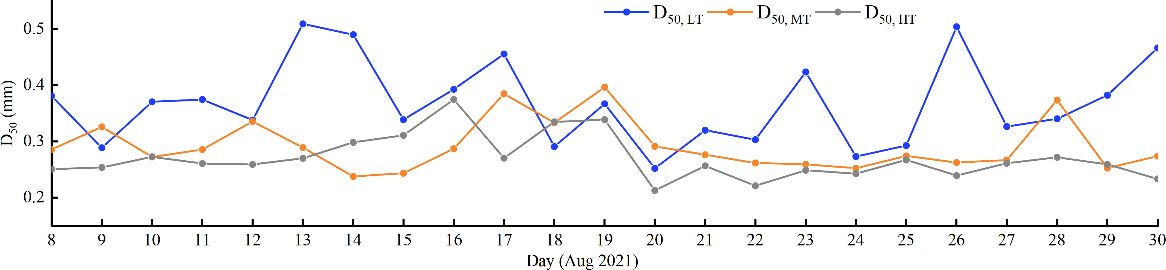
Figure 3 Temporal distribution of D₅₀ of HT, MT, and LT.

3.2 Hydrodynamics

Incident wave energy at the study area during field observations was characterized by moderate to low to medium energy (H_s >0.5 m for moderate wave conditions and H_s<0.5 m for low energy wave conditions (Masselink et al., 2006; Masselink et al., 2007)). The significant wave heights in deep water (H_{s, deep}) during the medium wave energy period (MEP I: 00:00 on August 8 to 7:00 on August 17; MEP II: 18:00 on August 20 to 23:00 on August 29) were 0.51–1.03 m and 0.46–0.97 m, respectively, whereas H_{s, deep} during the low wave energy period (LEP: 8:00 on August 17 to 17:00 on August 20) ranged 0.39 m–0.50 m. As shown in Figure 4, wave energy is mainly concentrated in the narrow frequency domain on both sides of the spectral density peak, and the spectral density peak of LEP is significantly smaller than those of MEP I and MEP II.

FIGURE 4

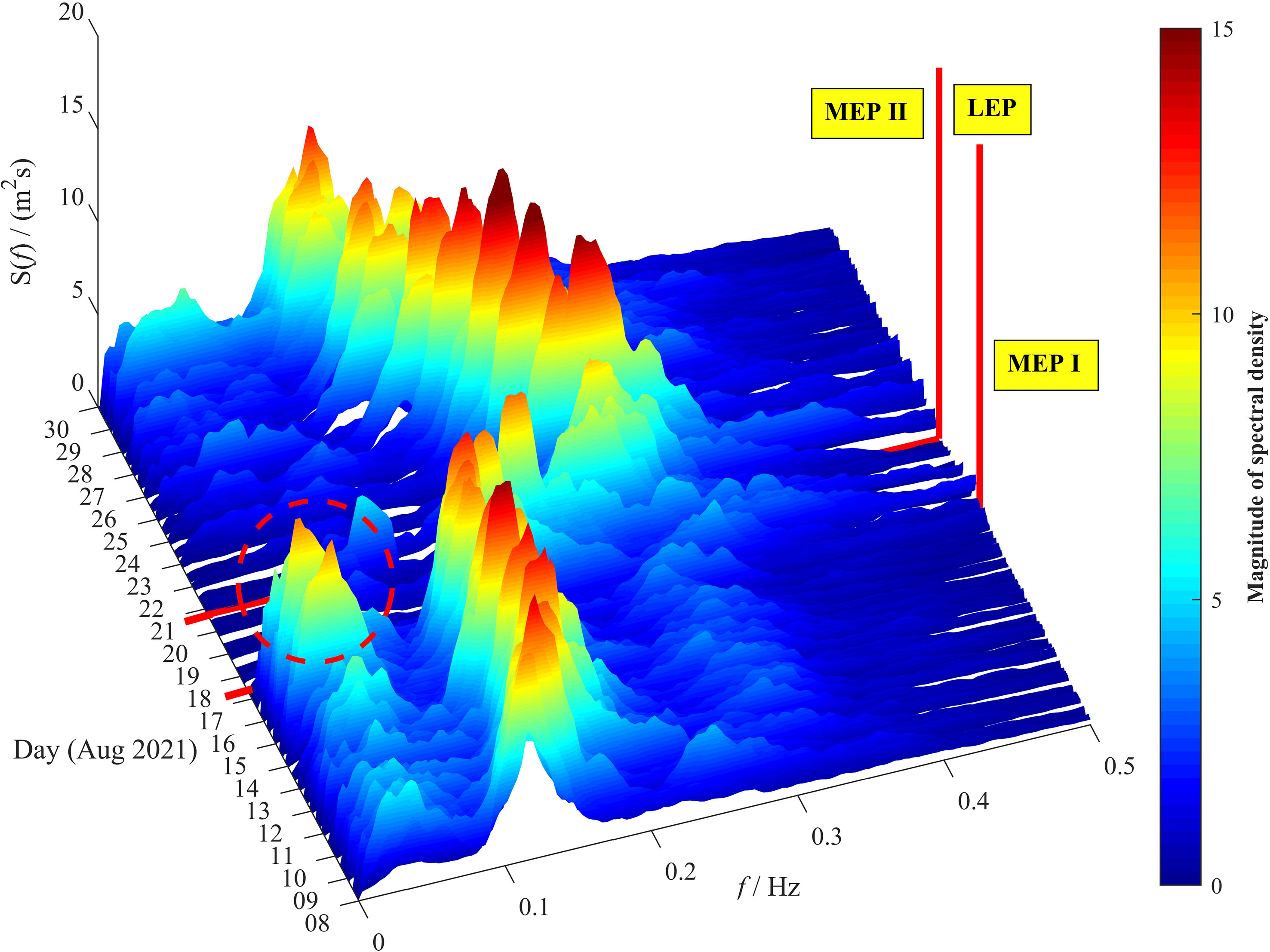
Figure 4 Three-dimensional plot of wave energy frequency-time. The red solid line indicates the wave energy period boundary, and the red dotted circle indicates the low frequency (<0.04 Hz) where the spectral density is significant. Wave energy measured by the RBR solo³ tide and wave recorder deployed at site B2.

In MEP I and MEP II, the significant wave height in the surf zone (H_{s, surf}) was influenced by water level changes, but to different degrees (Figure 5B). Throughout MEP I and MEP II, the waves in the surf zone were highly sensitive to depth (h). The H_{s, surf} of LEP was poorly affected by h, and the recorded H_{s, surf} values were small. H_{s, surf} were mostly smaller than H_{s, deep} throughout the field observation, indicating that the incident waves were subjected to topography of study area (shoaling and dissipation by bottom friction), which attenuated the wave energy (Figure 5B). Figure 5C shows that the deep-water wave direction was close to shore-normal, close to the onshore direction, until August 18, with a brief period of SSE and ESE between August 18 and 23, eventually changing to ESE. The mean wave period calculated using the zero up-crossing method ranged from 2.24 s to 6.85 s, close to that observed at the Zhapo ocean station.

FIGURE 5

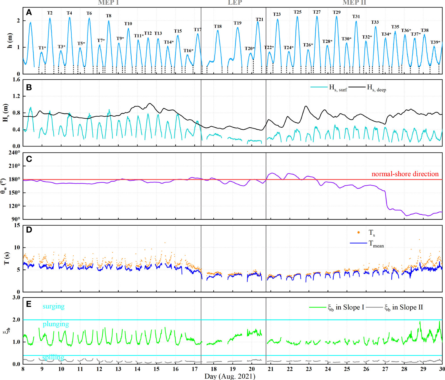
Figure 5 (A) Depth (h); black text and dashed lines mark 39 tidal cycles. (B) Significant wave height in the surf zone (H_{s, surf}) and in deep water (H_{s, deep}). (C) Wave direction in deep water (${\theta }_c$); horizontal line indicates the normal-shore direction (180°). (D) Mean wave period (blue solid line) and peak wave period (orange dots) within the surf zone. (E) Surf similarity parameters (ξ_b); two cyan horizontal lines indicate ξ_b = 0.4 and 2.0, respectively.

Using equation (1), ξ_b was calculated separately for slopes I and II. Throughout the field observations, slope I was dominated by a plunging breaker whereas slope II was dominated by a spilling breaker (Figure 5E). The ξ_b value for slope I fluctuated considerably, whereas the ξ_b values for slope II were relatively stable. There are large-scale vortices and turbulence in the water bodies of both plunging and spilling breakers, but the vortex and turbulence of the spilling breaker only occur on the surface part and the plunging breaker can penetrate deep into the seabed. Therefore, the bottom sediment may be suspended to the entire water column where the plunging breaker occurs, whereas at the spilling breaker, the bottom sediment is suspended to a limited height (Battjess, 1974; Galvin, 1968). The variations in ξ_b values show that sediment movement is more intense in slope I than in slope II.

Figure 6 shows the 5-min time-averaged cross-shore (U; blue line) and along-shore (V; red line) flow velocities and the depth recorded at sites B2 and C. The recorded velocities show that, in time, the changes in U and V of MEP I are significantly larger than those of MEP II and LEP and the changes in U and V of MEP II are similar to those of LEP. In space, the changes in U and V of B2 and C are similar. Figures 6C, D show the same range of θ_c at sites B2 and C, mainly between −90° and 0°, indicating that the main flow direction of the surf zone is between E and S. At high tide levels, flows with θ_c >0° occur but for shorter durations.

FIGURE 6

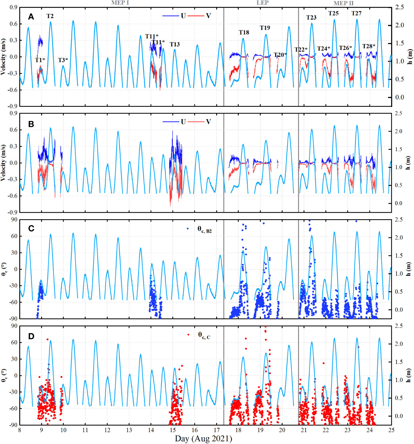
Figure 6 Five-minute time-averaged cross-shore velocity (U) and along-shore velocity (V) recorded by EM-B2 (A) and EM-C (B), respectively. Mean flow angle of B2 (C) and C (D), indicated by blue and red dots, respectively. The light blue line indicates the water depth.

The Eulerian measurement method was used in the experiment, and the EM was arranged at a fixed height in the surf zone. As the water level increased or decreased, the position in the water column of the EM changed accordingly. Influenced by the tidal water level, the velocity recorded by EM also showed a trend of variation with h. The EM recorded a higher velocity when h was smaller (Figures 6A, B). As h increased, the distance between the EM and the free surface increased and the velocity decreased. At a certain depth, the velocity approached 0 m/s, indicating that the water body at that depth was close to the stationary state.

3.3 Bed level elevation changes

3.3.1 Bed level elevation changes under different tidal cycles

The PAA recorded the bed level change at the beginning and end of each pulse, and the BLE at different sites was marked with the instrument sites (Figure 7). The PAA-A recorded the longest BLE change, and the change in the BLE at other sites was the same as that at site A (except BLE-C after day 19). The BLE at site A represents the change in bed level in each tidal cycle (defined as a tidal cycle from one low tide to the next). The BLE at site A experienced 39 tidal cycles (Figure 5A), among which T1*–T6 and T24*–T29 were in the spring tides; T7*–T10, T18–T23, and T30*–T37* were in the middle tides; and T11–T17 and T38–T39* were in the neap tides (Table 1). Dongdao Beach has an mixed semidiurnal tide type, with two high tides and low tides in a day, but the tidal levels that can be reached by the two highest tides are different (the “highest tide” and “sub-highest tide” are defined as the tidal cycle that reaches the highest and second highest tide levels, respectively, in a mixed semidiurnal tide, sub-highest tide marked with *) and 19 out of 39 tidal cycles containing the sub-highest tide (Figure 5A).

FIGURE 7

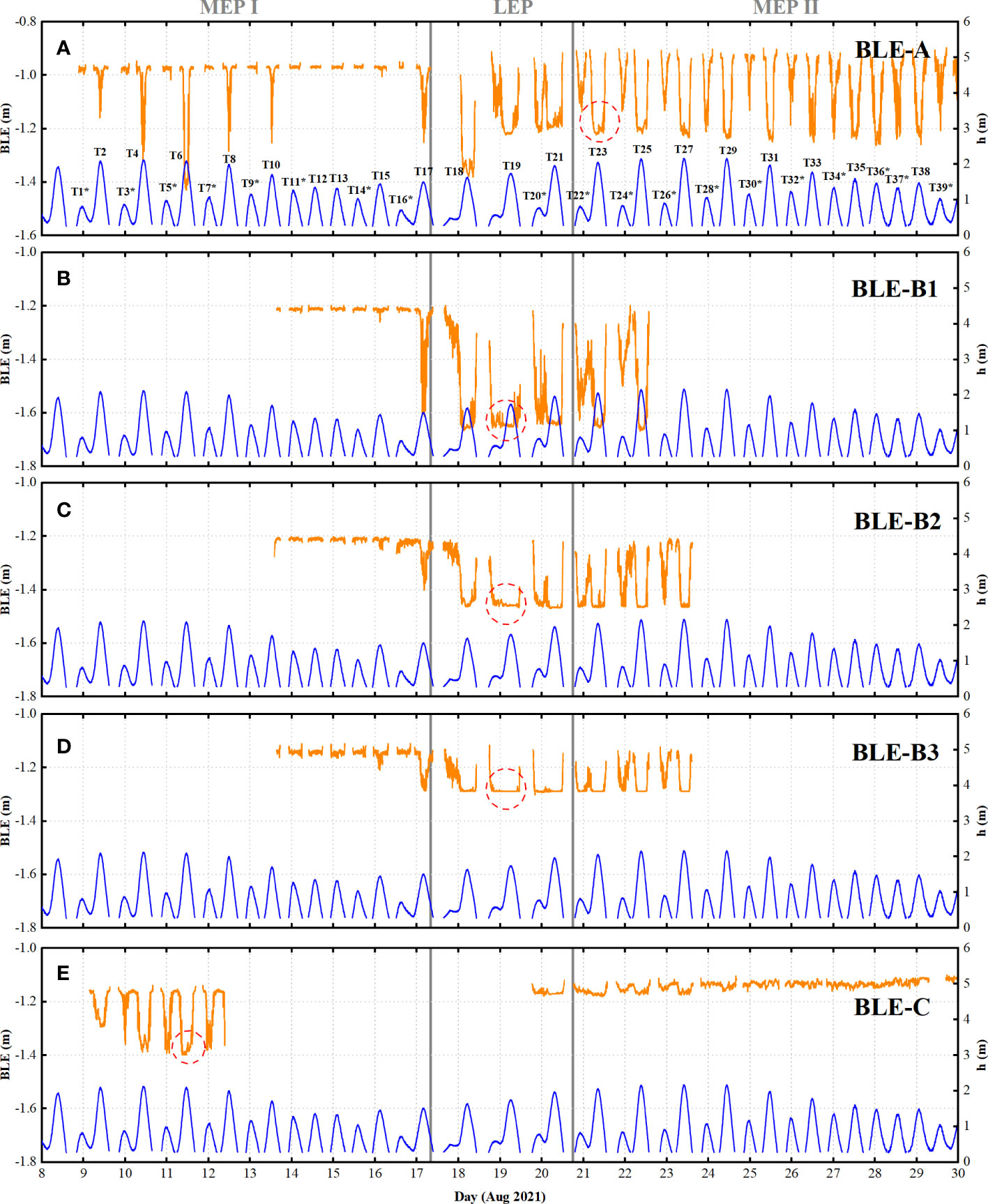
Figure 7 Five-minute time-averaged BLE recorded by PAA, BLE-A (A), BLE-B1 (B), BLE-B2 (C), BLE-B3 (D) and BLE-C (E) represent bed level elevation changes at sites A, B1, B2, B3, and C, respectively. Each red dashed circle marks an example of a "relatively stable" period of bed level elevation.

TABLE 1

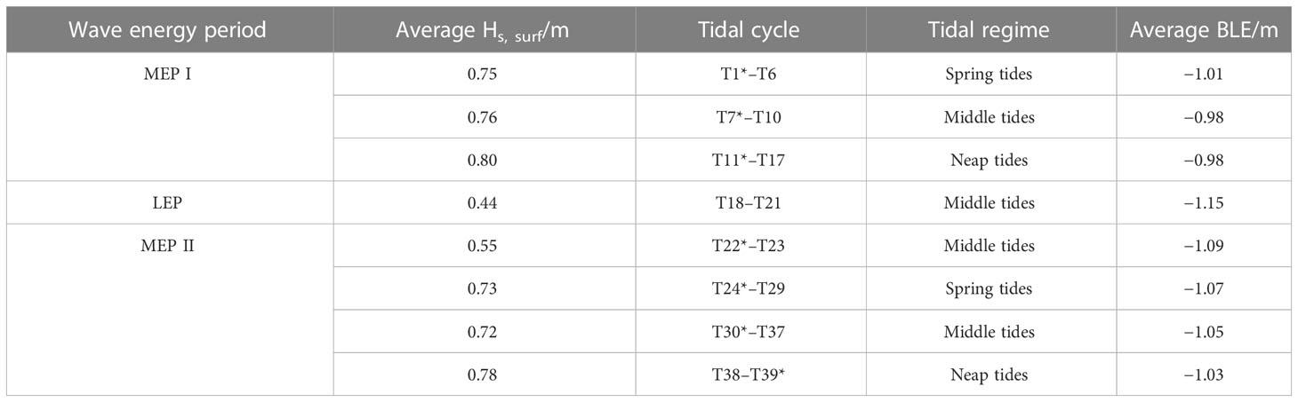
Table 1 Tidal cycle statistics under different wave energy periods.

By comparing the tidal cycle-averaged BLE, temporal variations in the bed level could be identified (Pang et al., 2021). Figure 8A shows that the tidal cycle-averaged BLE maximum (=-0.958 m) was at T30, located in MEP II, and the average bed level was the highest during this cycle. The tidal cycle-averaged minimum BLE occurred at T18 (=−1.309 m), located at the LEP, where the average bed level was the lowest. In all 39 tidal cycles, the BLE relative to the former tidal cycle ranged from −0.279 to +0.18 m. The tidal cycles of different high tides per day have different effects on the BLE. The BLE decreases in the highest tide cycle and increases in the sub-highest tide cycle; thus, the BLE shows an oscillating distribution relative to the former tidal cycle (Figure 8B). Figure 9A shows the probability distribution of the BLE relative to T1 for 2 days, which contains two highest tides and two sub-highest tides. The BLE distributions of T22* and T26* were inclined in the positive elevation direction, indicating that the BLE was likely to be higher than the initial bed level under the action of this tidal cycle. The BLE distributions of T23 and T27 were inclined in the negative elevation direction, and the elevation change was larger (relative to T1, which was more than 0.2 m). Such an elevation change will offset the accretion of the bed level during the sub-highest tide and cause beach erosion.

FIGURE 8

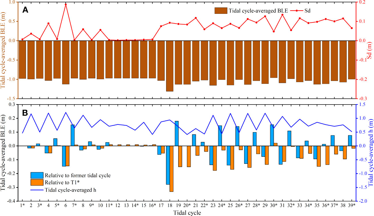
Figure 8 (A) Tidal cycle-averaged BLE (yellow bars) and standard deviation of tidal cycle-averaged BLE (red solid line). (B) Tidal cycle-averaged BLE relative to former tidal cycle (blue bars), tidal cycle-averaged BLE relative to T1* (orange bar), and tidal cycle-averaged depth (solid blue line).

FIGURE 9

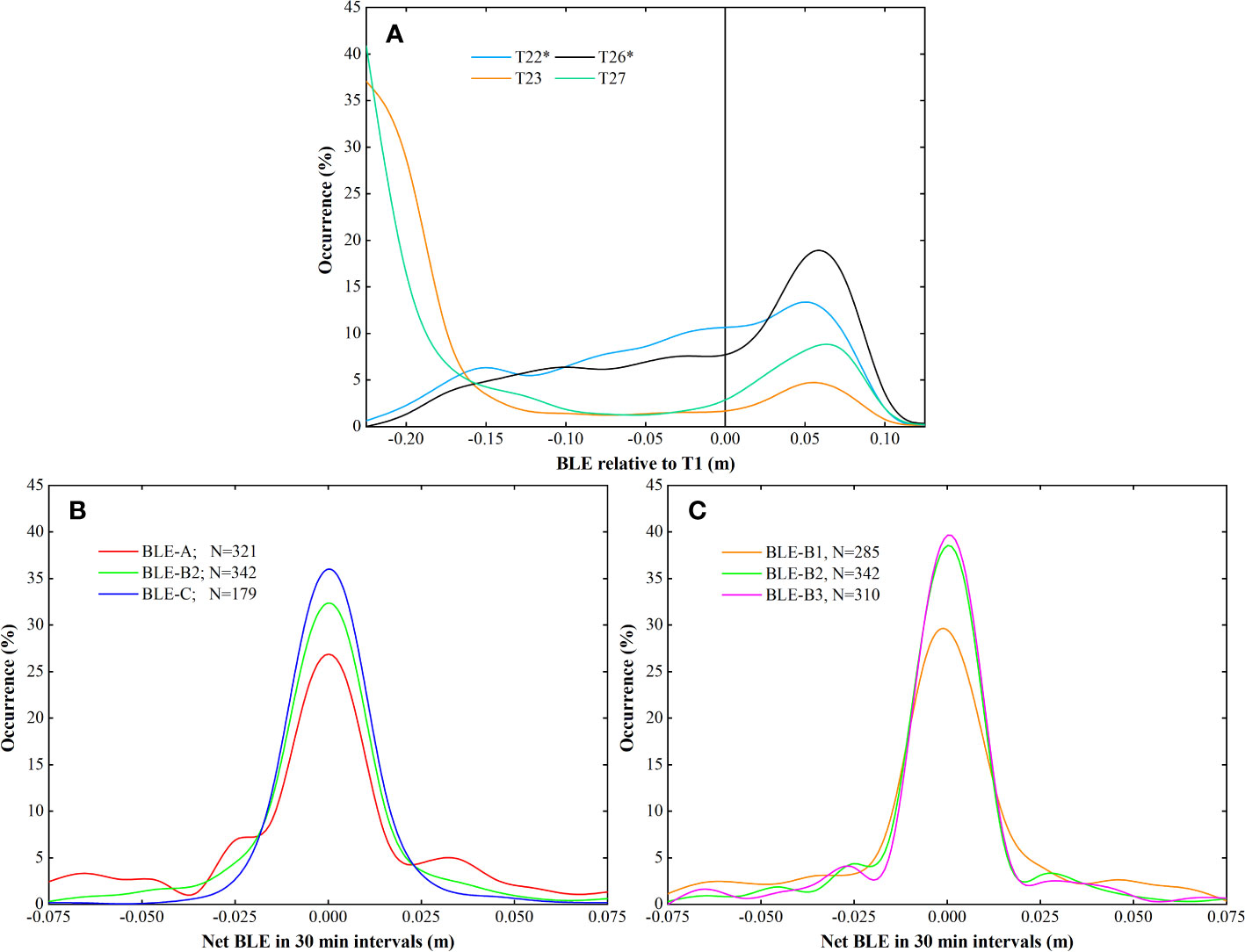
Figure 9 (A) Probability distribution of BLE relative to T1. (B) Probability distribution of net BLE for cross-shore. (C) Probability distribution of net BLE for along-shore.

3.3.2 Bed level change at different sites

BLE-A, -B2, and -C were located at three sites in the cross-shore direction. Except for T11*–T16*, BLE-A exhibited a relatively large change in each tidal cycle. On the intra-tidal scale, the BLE decreased during flood tide and increased during ebb tide. BLE-A of T11*–T16* was relatively stable without large erosion and accretion events, similar to other tidal cycles. In contrast to the large changes in the BLE during flood or ebb tides, the net BLE change was close to zero in the high-water regions of some tidal cycles (Figure 10). This indicates that when the depth is large, there is a “relative stability” period at the lowest BLE (Figure 7). The variations in BLE-B2 recorded by PAA-B2 are similar to those in BLE-A in the same period, but Figure 10A shows that in T17–T27, net BLE-B2 is smaller than net BLE-A. BLE-C has a longer duration of “relative stability” in T2–T8. BLE-C after T20* tends to be stable, and the maximum net BLE-C can only reach 0.032 m (Figure 10A), which is significantly smaller than the two cross-shore sites A and B2, indicating that no large erosion or accretion events have occurred at site C since then. The changes in BLE-B1, -B2, and -B3 of T11*–T16* are similar to those in BLE-A in the same period, and the changes in the net BLE of the three sites are small. BLE-B1, -B2, and -B3 of T17–T25 also decreased during flood tide and rose at ebb tide, but the magnitude of the net change in BLE was different (Figure 10B).

FIGURE 10

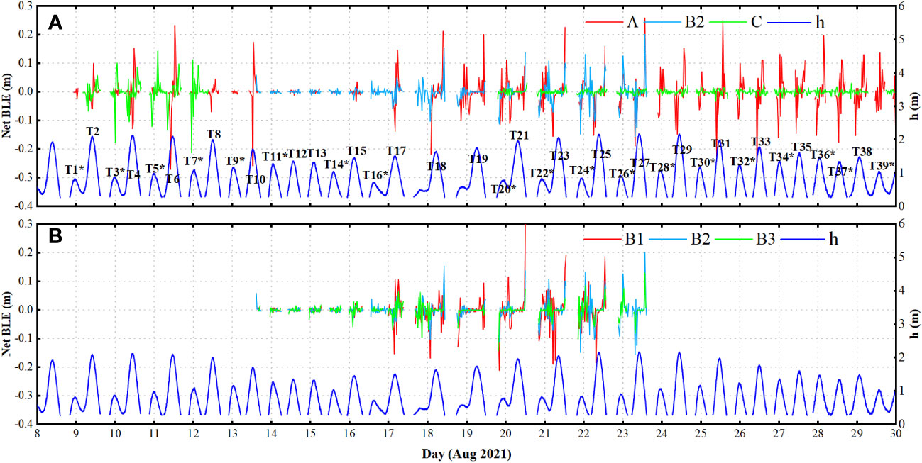
Figure 10 (A) Net BLE of cross-shore measurement sites. (B) Net BLE of along-shore measurement sites.

The probability distributions of 5-min-averaged net BLE at 30-min intervals at different sites in T11*–T27 were calculated to compare the distribution of BLE changes at different locations (Figures 9B, C). The data collection time ranges for PAA-A, -B1, -B2, -B3, and -C overlapped at T11*–T27. Based on the BLE changes at the same time at the other four sites, it was assumed that BLE-C remains stable during the missing time. The numbers of samples retained in BLE-A, -B1, -B2, -B3, and -C were 321, 285, 342, 310, and 179, respectively. The probability distributions of net BLE changes at all sites were nearly normal (goodness-of-fit values significant at the 95% level based on a χ² test statistic with 12 degrees of freedom). Large changes of up to approximately 0.035 m were observed, but only by less than 5%. The change in the net BLE is mainly concentrated in the range of less than 0.005 m, whereas the tidal cycle-averaged BLE relative to the former tidal cycle shows a change of ±0.1 m (Figure 8B), indicating that a few erosion and accretion events caused the “large” changes in BLE (Puleo et al., 2014); Figure 7 shows the rapid decrease (increase) in bed elevation at the flood tide (ebb tide).

Figures 9B, C show that within the range of BLE change of less than 0.005 m, the order of percent occurrence is C, B2, A in the cross-shore direction and B3, B2, B1 in the along-shore direction, with the opposite percent occurrence for BLE changes greater than 0.02 m. “Large” net BLE has an important effect on beach surface erosion and accretion. The higher percent occurrence of large BLE changes indicates high possibility for sediment movement. Therefore, in the cross-shore direction, there was more sediment movement at A, followed by B2, and at C, it is the smallest; in the along-shore direction, the sediment movement intensity of B1 to B3 decreases.

4 Discussion

4.1 Hydrodynamic and bed level elevation responses in the surf zone

Storms can have strong erosive effects on beach berms and backshore dunes (Stockdon et al., 2007; Silva et al., 2016). A field observation revealed that the sand bar at the study area on July 15 disappeared after Storm “Cempaka”. The post-storm beach profile has a steeper slope above the MSL (slope I), where the breaker type is predominantly plunging, and a gentle slope between the MSL and mean low water springs (MLWS) (slope II), where the breaker type is spilling, suggesting stronger wave agitation of the sediment at high tide levels. Except on August 18, the D₅₀ of HT was greater than that D₅₀ of LT (Figure 3), which also indicates that slope I had stronger hydrodynamic conditions.

Wave conditions during field observations can be divided into three periods based on wave energy: MEP I, LEP, and MEP II. The energy of MEP I and MEP II not only is distributed in the high-frequency oscillations of 0.1–0.3 Hz but also has peaks of energy at low frequencies (<0.04 Hz) (Figure 4), and LEP has no energy peaks at low frequencies. The low-frequency wave energy is small; however, it affects the transport of seafloor sand layers and has a significant impact on the shape of the nearshore beach (Mendoza et al., 2020).

The tidal water level is an important factor that affects the hydrodynamics of the surf zone. The tidal modulated depth limits the incident wave height through energy dissipation and wave breaking, and the tide has an impact on the bed level change through this limitation (Kroon and Masselink, 2002). Under different wave energy conditions, depth has different effects on the modulation of H_{s, surf}. The wave energy of MEP I is the highest. In MEP I, wave sensitivity to depth is the highest and H_{s, surf} and h show a positive correlation (slope decreases after h >1.37 m, the relative decrease in the sensitivity of H_{s, surf} to depth) (Figure 11A), indicating that H_{s, surf} at this stage is likely to be close to the limit of wave breaking. In LEP and MEP II, the same situation occurs at h<0.5 m and h<1.1 m, respectively. The long-term action of the breaking wave in the surf zone causes the BLE to change significantly, which can also explain the fact that the maximum value of the net BLE change in each wave energy period in Figure 11B occurs near the depth corresponding to the maximum value that can be reached by H_{s, surf} (the water level corresponding to the solid circle in Figure 11A). The limits that can be reached by H_{s, surf} in LEP and MEP II are smaller than those in MEP I, indicating that the breaker depth indices (γ_b, ratio of wave breaking height to the depth at breaking) in LEP and MEP II are smaller than those in MEP I. In LEP and MEP II, the modulation effect of h on H_{s, surf} disappeared when h increased to a certain value.

FIGURE 11

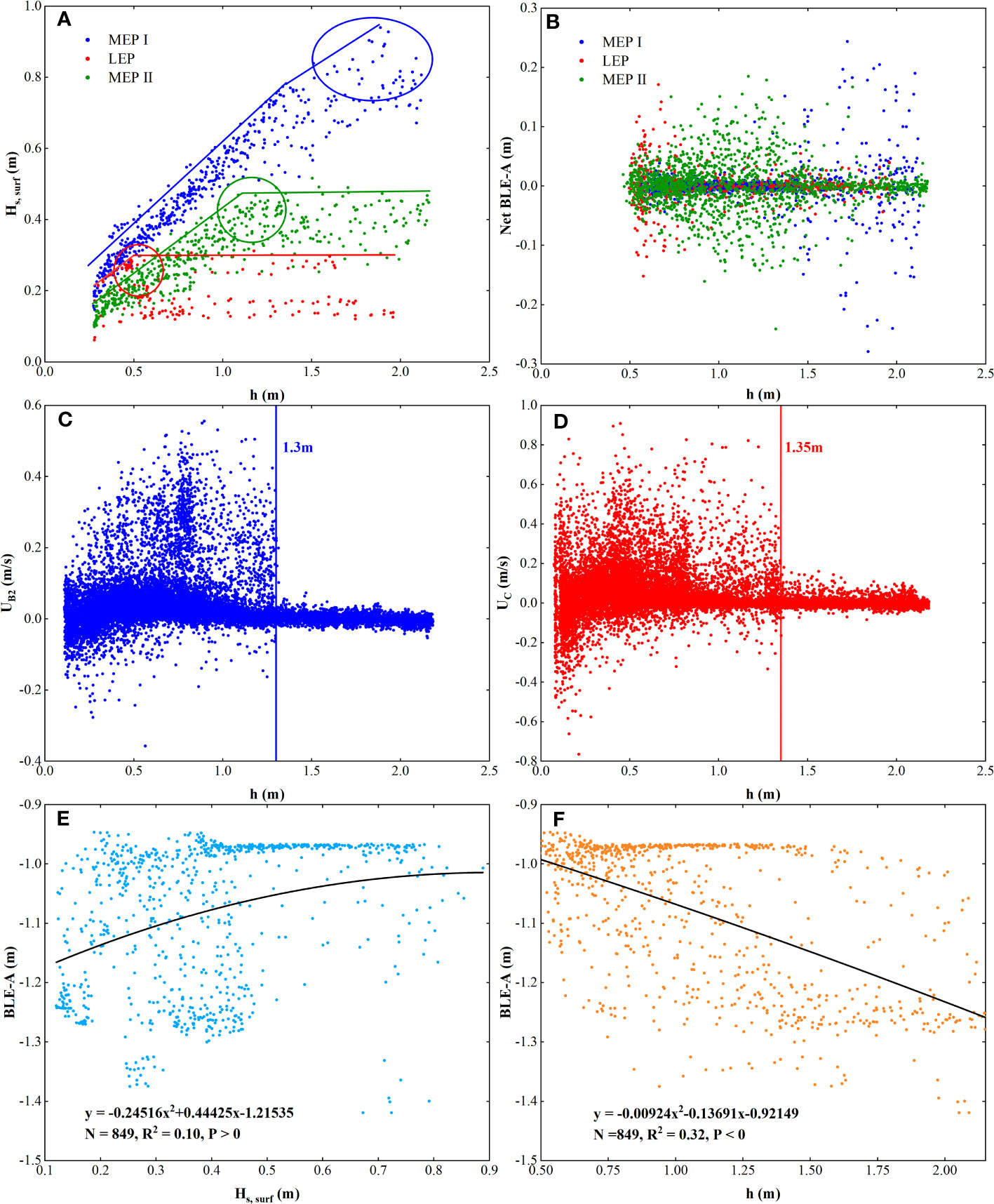
Figure 11 (A) Scatter plot of H_{s, surf} with h; the solid lines indicate the h limitation of H_{s, surf}, and the circles indicate the maximum value that H_{s, surf} can reach at each period. (B) Scatter plot of net BLE and h for different wave energy periods. (C) Scatter plot of the cross-shore velocity (U_B2) at site B2 with (h) (D) Scatter plot of the cross-shore velocity (U_C) at site C with (h) The vertical lines in (C, D) are the estimated breakpoints. (E) Scatter plot of BLE-A with H_{s, surf}. (F) Scatter plot of BLE-A with (h) The black lines in (E, F) are the fitted lines.

The BLE during field observations was also modulated by tides (except for T11*–T16*), and the bed level changes showed a decrease at flood tide and an increase at ebb tide, which may be related to the very low frequency (VLF) pulsation of the BLE (see analysis in Section 4.3). Figure 10 shows that the magnitude of change in the net BLE in the high tide region was significantly reduced compared with that during flood and ebb tides. At the same time, the Eulerian velocities of B2 and C were close to 0 in the high-tide region (Figures 6A, B). Figures 11C, D show the scatter plots of cross-shore velocity and h at B2 and C, with h = 1.3 m and 1.35 m as breakpoints, respectively, with the difference between the two breakpoints almost equal to the difference in the instrumental height between PAA-B2 and PAA-C (0.048 m). The cross-shore velocity values before the breakpoint were scattered throughout the coordinate system, and those after the breakpoint were concentrated around U = 0. This suggests that the underwater flow slows when a certain depth is reached. Sediment transport is affected by flow velocity, and the “relatively stable” period of BLE in the high-tide region is related to the slowing of underwater flow velocity.

The changes in BLE-A, -B1, -B2, and -B3 were not affected by tidal modulation during T11*–T16*, and no large erosion or accretion events occurred in these tidal cycles (Figures 7A–D). Compared with the other tidal cycles, there were no particular differences in wave height and tidal variations in the T11*–T16* period (Figure 5), but the waves appeared to have higher energy at low frequencies during this period (Figure 4, red dashed circle). Coastal low-frequency waves reflect sediment transport currents (Osborne and Greenwood, 1992); thus, the variations in the characteristics of BLE during T11*–T16* are likely caused by the strong sediment transport currents that cause the input and output sediment fluxes to be exactly equal to the waves rolling up the sediment from the seafloor, resulting in small BLE variations being recorded at each site.

The percent occurrences of BLE changes of different magnitudes showed variations. A larger net BLE variation indicates high possibility for sediment movement. The percent occurrence of large net BLE changes at sites A and B1 was the highest and gradually decreased offshore and away from the headland, respectively (Figures 9B, C), indicating that A and B1 had higher potential for sediment movement. The mean flow direction indicates the direction of sediment transport. The θ_c values of B2 and C were mainly between −90° and 0°, indicating that the sediment moved onshore and away from the headland in the cross- and along-shore directions, respectively. Depending on the sediment transport and flow direction, under future normal wave conditions, site C may have more stable sediment movement, which re-forms a sand bar; site A may have more sediment moving onshore, thus forming a channel; and the BLE from B1 to B3 (away from the headland) may rise in sequence, as confirmed by the along-shore profile of the beach (Figure 2D).

At present, there are two representative theories on the formation and migration of sand bars: forced response theory (Holman and Sallenger, 1993) and self-organization theory (Stive and Reniers, 2003). The formation of sand bars may be driven by hydrodynamic forcing and the self-organization process of sand bars (Coco and Murray, 2007). The beach profile first needs to reach a critical condition for its change under hydrodynamic forcing and then evolves continuously under the interaction between the seabed and the fluid (Caplain et al., 2011). Sandbar changes on study area were affected by the combined effects of these two mechanisms. When the velocity of underwater fluid is less than a certain value, the BLE changes slightly (“relative stability” period of the BLE), indicating that the formation of sand bars cannot respond to the hydrodynamic force at this time. When the hydrodynamic force reaches a critical value, the BLE begins to change greatly and a positive feedback occurs between the bed level fluctuation and circulation and related sediment transport (Falqués et al., 2008). Owing to the self-organized coupling between the bed level and hydrodynamics, the surf zone forms a bar-channel topography.

4.2 Influence of wave energy conditions and tidal regime on beach topography

The variations in the tidal cycle-averaged BLE exhibited different characteristics under different wave energy conditions and tidal regimes (Table 1). The two medium wave energy periods (MEP I and MEP II) experience a complete astronomical tide cycle (the tidal regime continuously includes spring, middle, and neap tides), whereas the low wave energy period (LEP) experiences only middle tides. The effects of wave energy and tidal regime on BLE changes were analyzed separately using the control variable method (Table 1). Figures 11E, F show the scatter plots of BLE-A and H_{s, surf} and h, respectively, which are positively and negatively correlated with H_{s, surf} and h, respectively. Figure 12A shows the average BLE of T7*–T10, T22*–T23, and T30*–T37*, which are located in three wave energy periods, respectively, and are in the order of energy magnitude MEP I, MEP II, and LEP, and the tidal regime is under middle tides (Table 1). The LEP has the smallest average BLE, followed by MEP II and MEP I, suggesting that the transition from low to medium wave energy on study area favors accretion of the beach surface. This is in contrast to the relationship between the bed surface and wave energy under non-storm-influenced wave conditions, which is the erosion of the bed surface under relatively high-energy wave conditions (Pang et al., 2021). This result is consistent with the macroscopic survey results of Yu et al. (2013) on the beach profile after a typhoon. In addition, the average BLE in MEP I under spring tide and neap tide is greater than that in MEP II (Figure 12B), which also proves the positive effect of wave energy on bed-level accretion. This result explains the positive correlation between BLE-A and H_{s, surf} in Figure 11E.

FIGURE 12

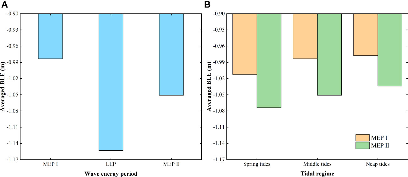
Figure 12 (A) Average BLE under different wave energy periods at middle tides. (B) Average BLE under different tidal regimes in the same wave energy period.

The calculation of the average BLE under different tidal regimes in MEP I and MEP II (Figure 12B) showed that the average BLE gradually increased as the tidal regime changed from spring tide to neap tide, indicating that the smaller tidal range is more conducive to the development of beach accretion. This explains the negative correlation in the scatter plot of BLE-A and h in Figure 11F, reflected by the increase in the tidal cycle-averaged BLE at the “sub-highest tide” compared with the “highest tide”. In addition, the analysis of the 2-day mixed semidiurnal tide showed the opposite effects of two different tidal cycles in the mixed semidiurnal tide on the BLE. Beaches are eroded at the “highest tide” tidal cycle and accretion at the “sub-highest tide” tide cycle. The interaction of “highest tide” and “sub-highest tide” together influences beach changes within a mixed semidiurnal tide.

4.3 Very-low-frequency pulsation in the surf zone

Spectral analysis is a mature method for studying wave structures and is widely used in the study of surf zones (Puleo et al., 2014; Hu et al., 2022). To analyze the depth, velocity, and BLE during beach recovery, taking T8 with the longest tidal cycle duration as an example, the depth and velocity were resampled to the recording frequency corresponding to the PAA, and the bed level during this cycle was fully influenced by depth and velocity. Figures 13A–C show the depth, velocity, and BLE spectra at site B2, respectively. The energy density of all three spectra increased, followed by a decay.

FIGURE 13

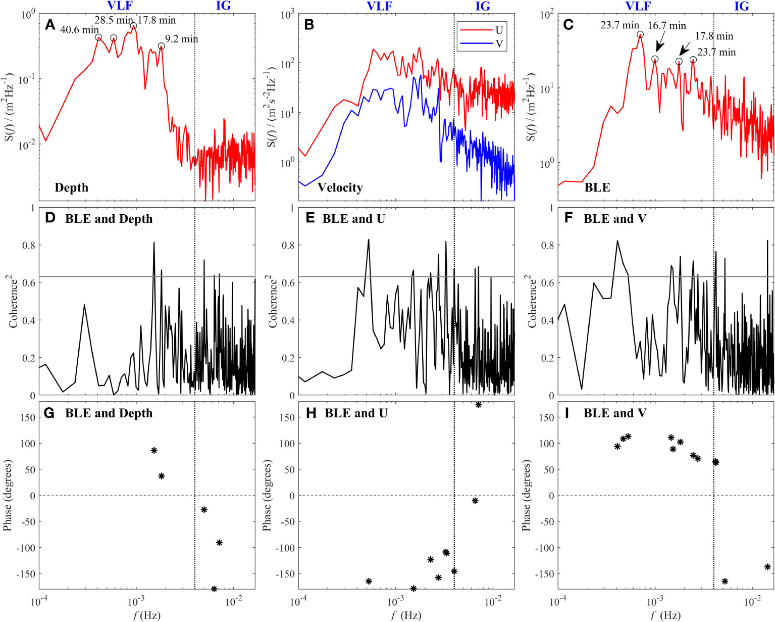
Figure 13 (A–C) Spectra of h, U (red solid line), V (blue solid line), and BLE; black circles mark the dominant peaks of spectral density. (D–F) Squared coherence of BLE and h, BLE and U, and BLE and V, respectively; horizontal gray solid lines indicate the squared coherence at the 95% confidence level. (G–I) Cross-spectral phases of BLE and h, BLE and U, and BLE and V, respectively; the phases are shown only when the squared coherence is significant (>95%). The very low frequency band (f<0.004 Hz), the infragravity band (0.004< f<0.04 Hz), and the vertical gray dashed line indicate 0.004 Hz, delineating the very low frequency (VLF) and the infragravity band (IG).

The depth spectra (Figure 13A) show that the energy density peaks are mainly concentrated in the VLF band (f<0.004 Hz) and the dominant peaks are 40.6, 28.5, 17.8, and 9.2 min, respectively. The depth spectra decayed rapidly after a peak period of 9.2 min and remained stable in the infragravity (IG) band. These VLF pulsations are the dominant features of the depth spectra, and their corresponding energy density peaks are 26.3 times higher than those within the IG band. Compared with the depth spectra, the VLF pulsation of the velocity spectra had no clear dominant peaks (Figure 13B). The peaks of the cross-shore velocity spectra were not synchronous with those of the along-shore velocity spectra, but the difference between them was small. The peak energy density of the velocity spectra reached its highest value in the VLF band, which was 2.5 times the peak energy density in the IG band. In contrast to the depth spectra, in the attenuation part of the energy density, the velocity spectra exhibited an almost linear attenuation with an increase in frequency and the attenuation slope of the along-shore velocity spectra was larger than that of the cross-shore spectra. The BLE spectra had dominant peaks at 23.7, 16.7, 9.5, and 6.8 min, all within the VLF band. Compared with the velocity spectra, the BLE spectra showed a large VLF peak, 3.6 times that of the IG peak, with a decay trend similar to that of the velocity spectra (Figure 13C).

Cross-spectral analysis was performed to determine the squared coherence between the depth, velocity, and BLE responses. The cross-spectral calculation parameters are the same as those described above Section 2.3.1. The horizontal gray lines in Figures 13D–F represent the 95% significance level. For the T18 example, the squared coherence peaks at BLE&h only exceed the 95% significance level at 10.9 min and 9.2 min and the squared coherence peak at 9.2 min is consistent with that observed in the depth spectra. The number of squared coherence peaks for which BLE&U and BLE&V exceed the significance level increases relative to BLE&h. There are other square coherence peaks above the 95% significance level in the IG band, but spectral analysis shows that the energy density is mainly concentrated in the VLF band (Figures 13A–C) and the energy density of these peaks is lower; therefore, the impact on BLE changes is limited. Figures 13G–I show the phase estimates when the squared coherence exceeds the significance level. In the VLF band, the phases of BLE&h and BLE&V are both positive and the phase of BLE&U is negative, indicating that the BLE response leads to depth and along-shore velocity and lags the cross-shore velocity. The phase difference between the squared coherence peaks of BLE and depth is close to 90°, indicating that at these frequencies, BLE and depth change in opposite directions with time between the adjacent BLE extrema and depth extrema. The BLE is almost asynchronous, with a cross-shore velocity of approximately 180°. The 180° phase lag indicated that the BLE decreased when the cross-shore velocity increased. This differs from the results of a previous study on dissipative beaches under normal wave conditions. Puleo et al. (2014) reported that under normal wave conditions, the wave spectra of depth, velocity, and BLE and their cross-spectra showed significant peaks at low frequencies and that there were some dominant peaks at the same frequency between the wave spectra and between the cross-spectra. However, during recovery, dominant peaks in both the wave spectra and cross-spectra were observed at different frequencies. Furthermore, Puleo et al. (2014) observed that the BLE response lagged both depth and velocity at significant squared coherence peaks in the low-frequency band, with the phase difference between BLE&h and BLE&U being approximately 180° and 90°, respectively. During the recovery process, the BLE change led to depth, indicating that the BLE change was more active at this time.

4.4 Hydrodynamic forcing during the beach recovery process

Vousdoukas et al. (2012) suggested that during a storm event, the antecedent morphological state can initially be the dominant controlling factor of beach response, whereas the hydrodynamic forcing, and especially the tide and surge levels, controls storm impact during the later storms. Specifically, the beach recovery process is that the beach morphology formed in the storm event readapts to ordinary dynamic conditions with landform changes (Ge et al., 2017) and hydrodynamic features play an important role in this process. Yu et al. (2013) investigated the beach profiles and sediment characteristics of two headland beaches under two different wave energy conditions after a typhoon and found that the high-wave-energy-exposed beach recovered quickly, with significant post-storm accretion of fine- to medium-grained sand, whereas the low-wave-energy beach showed little evidence of sand accretion or recovery in the same 4 months after the typhoon, with only minor changes in the beach profile. Ge et al. (2017) also found that after typhoon Rammasun, slight geomorphic changes were detected in the backshore and dunes of Yintan Beach in Beihai, China, when there was a lack of persistent strong wave activity, which suggests that longer time was required for beach recovery because of such wave conditions. The BLE changes of the study area had the same characteristics. In the LEP with the lowest wave energy, the average BLE of beach was the lowest. In MEP II with the highest wave energy, the average BLE of the beach was the highest. This suggests that during the beach restoration phase, high wave energy favors an increase in beach bed level elevation and accelerates beach accretion. The high-energy waves are enough to bring sediments from near-shore areas back to their pre-storm positions on the beach, elevating the BLE. However, in low-energy conditions, the effects of waves are not strong enough to bring offshore sediments to the beach.

Egense (1989) divided the recovery of a headland beach in Southern California, USA, into two phases. In the first phase, beach can recover nearly half of the eroded volume of sand within a few days to tens of days following the storm, whereas the recovery rate in the second phase slowed down and continued for a longer time than the first phase (Birkemeier, 1979; Egense, 1989; Wang et al., 2006). The BLE changes in the study area were much obvious during the field observations, and the bar-channel topography was being formed. Dongdao beach can be considered to be in the first phase of beach recovery. The state of beach profile and sandbar recovery in the study area suggests that this phase will remain for some time. Beach replenishment and beach nourishment after storms need to focus on the first phase of beach recovery. At the same time, the hydrodynamic characteristics of the beaches should be further investigated and different coastal management strategies should be applied for different wave energy conditions. For high-energy beaches, interfering with their natural state is not recommended. For low-energy beaches, human intervention may be required due to the fact that beach recovery takes longer time.

4.5 Limitations and implications of the study

The field observations for this study began on the 19th day after the typhoon made landfall, and the beach had been recovering for some time. Affected by the residual waves after the typhoon, the beach recovery in the early stage was very small, so this study can reveal the topographic change characteristics of the surf zone in the early stage of beach recovery to a certain extent. Unfortunately, PAA-B1, -B2, -B3, and -C did not collect complete BLE data. In T11*–T27, the change trends of BLE-B1, -B2, and -B3 were very similar to those of BLE-A (Figure 7), so that BLE-A basically represented the bed level changes in the surf zone. The measurement time of PAA needs to be adjusted reasonably in future field observations to obtain the complete BLE variation of each site. The study investigated bed level elevation changes during beach recovery after storms and examined the effects of wave energy and tidal on bed level. This study also provides a reference for the next field observations of the surf zone in the short term after the storm.

5 Conclusions

Following storm Cempaka, a 21-day field observation was conducted in the surf zone of the Dongdao Beach in Hailing Island, China, and the high-frequency bed level elevation changes during the beach recovery were measured using five precision autonomous hydroacoustic altimeters. The purposes of the study were to investigate the variation characteristics of wave, current, tidal, and bed level elevation in the post-storm surf zone and to explore the influencing factors and their interactions during beach recovery. The study provides a reference for further research on the intrinsic mechanisms of beach recovery after storms around the world.

1. The average tidal-cycle BLE under medium-energy conditions was higher than that under low-energy conditions, and a relatively high wave energy was conducive to accretion on the beach surface. This is opposite to the effect of wave energy on beach accretion and erosion under normal wave conditions and is consistent with the results of previous research on beach profiles and sediments after typhoons.

2. When the tidal regime changed from spring tide to neap tide, the average tidal-cycle BLE gradually increased and a smaller tidal range was more conducive to beach accretion. During the “highest tide” and “sub-highest tide” tidal cycles within a mixed semidiurnal tide, the BLE decreased and increased, respectively, and the two tidal cycles canceled each other’s erosion or accretion, resulting in overall changes in the beach profile.

3. After the storm, the formation of sand bars in the surf zone was the result of the combined action of hydrodynamic forcing and self-organization of sand bars. Under future normal wave conditions, the beach forms a new bar-channel topography.

4. The BLE, depth, and velocity were most active within the VLF band in the post-storm surf zone. Cross-spectral analysis of BLE with depth and velocity also shows substantial squared coherent peaks in the VLF band. The BLE response during beach restoration leads to depth and along-shore velocity and lags the cross-shore velocity. During beach recovery, the response of BLE to depth contrasts with previous studies under non-storm conditions, showing that BLE changes are more active than under normal wave conditions.

Data availability statement

The raw data supporting the conclusions of this article will be made available by the authors, without undue reservation.

Author contributions

PH: visualization, methodology, investigation, and draft. ZL: conceptualization, methodology, review, and editing. CZ, DZ, RL, QS, and JT: investigation. YZ: review and editing. All authors contributed to the article and approved the submitted version.

Funding

This work was supported by the National Natural Science Foundation of China under Grant 42176167 and the Project of Enhancing School With Innovation of Guangdong Ocean University under Grant 18307.

Acknowledgments

Thanks are given to the satellite image data support from USGS and Google Earth. Thanks are also due to the ECMWF for providing the significant wave height and wave direction in deep water. The authors would like to thank all members of our team for their contributions in field observation, as well as the managers of Dongdao Beach for their assistance during the field observations.

Conflict of interest

The authors declare that the research was conducted in the absence of any commercial or financial relationships that could be construed as a potential conflict of interest.

Publisher’s note

All claims expressed in this article are solely those of the authors and do not necessarily represent those of their affiliated organizations, or those of the publisher, the editors and the reviewers. Any product that may be evaluated in this article, or claim that may be made by its manufacturer, is not guaranteed or endorsed by the publisher.

References

Agredano R., Cienfuegos R., Catalán P., Mignot E., Bonneton P., Bonneton N. (2019). Morphological changes in a cuspate sandy beach under persistent high-energy swells: Reaca Beach (Chile). Mar. Geol. 417, 105988. doi: 10.1016/j.margeo.2019.105988

CrossRef Full Text | Google Scholar

Battjes J. A. (1974). “Surf similarity,” in Proceeding 14th Coastal Engineering Conference (New York, NY), 466–479.

Google Scholar

Biausque M., Senechal N. (2019). Seasonal morphological response of an open sandy beach to winter wave conditions: The example of Biscarrosse beach, SW France. Geomorphology 332, 157–169. doi: 10.1016/j.geomorph.2019.02.009

CrossRef Full Text | Google Scholar

Birkemeier W. A. (1979). The effects of the 19 December 1977 coastal storm of beaches in North California and New Jersey. Shore Beach 47 (1), 7–15.

Google Scholar

Blott S. J., Pye K. (2001). GRADISTAT: a grain size distribution and statistics package for the analysis of unconsolidated sediments. Earth Surf. Proc. Land. 26 (11), 1237–1248. doi: 10.1002/esp.261

CrossRef Full Text | Google Scholar

Brenner O. T., Lentz E. E., Hapke C. J., Henderson R. E., Wilson K. E., Nelson T. R. (2018). Characterizing storm response and recovery using the beach change envelope: Fire Island, New York. Geomorphology 300, 189–202. doi: 10.1016/j.geomorph.2017.08.004

CrossRef Full Text | Google Scholar

Bruun P. (1954). Coast erosion and the development of beach profiles,” in Beach Erosion Board Tech. Memo Vol. 44 (Mississippi: U.S. Army Corps Engineers).

Google Scholar

Caplain B., Astruc D., Regard V., Moulin F. Y. (2011). Cliff retreat and sea bed morphology under monochromatic wave forcing: Experimental study. C. R. Geosci. 343 (7), 471–477. doi: 10.1016/j.crte.2011.06.003

CrossRef Full Text | Google Scholar

Ciavola P., Coco G. (2017). Coastal storms: processes and impacts (West Sussex: John Wiley &Sons).

Google Scholar

Coco G., Murray A. B. (2007). Patterns in the sand: From forcing templates to self-organization. Geomorphology 91 (3-4), 271–290. doi: 10.1016/j.geomorph.2007.04.023

CrossRef Full Text | Google Scholar

Coco G., Senechal N., Rejas A., Bryan K. R., Capo S., Parisot J. P., et al. (2014). Beach response to a sequence of extreme storms. Geomorphology 204, 493–501. doi: 10.1016/j.geomorph.2013.08.028

CrossRef Full Text | Google Scholar

Dodet G., Castelle B., Masselink G., Scott T., Davidson M., Floc’h F., et al. (2019). Beach recovery from extreme storm activity during the 2013–14 winter along the Atlantic coast of Europe. Earth Surf. Proc. Land. 44 (1), 393–401. doi: 10.1002/esp.4500

CrossRef Full Text | Google Scholar

Egense A. K. (1989). Southern California beach changes in response to extraordinary storm. Shore Beach 57 (4), 14–17.

Google Scholar

Falqués A., Dodd N., Garnier R., Ribas F., Machardy L. C., Larroudé P., et al. (2008). Rhythmic surf zone bars and morphodynamic self-organization. Coast. Eng. 55 (7-8), 622–641. doi: 10.1016/j.coastaleng.2007.11.012

CrossRef Full Text | Google Scholar

Galvin C. J. Jr (1968). Breaker type classification on three laboratory beaches. J. Geophys. Res. 73 (12), 3651–3659. doi: 10.1029/JB073i012p03651

CrossRef Full Text | Google Scholar

Ge Z., Dai Z., Pang W., Li S., Wei W., Mei X., et al. (2017). LIDAR-based detection of the post-typhoon recovery of a meso-macro-tidal beach in the Beibu Gulf, China. Mar. Geol. 391, 127–143. doi: 10.1016/j.margeo.2017.08.008

CrossRef Full Text | Google Scholar

Gervais M., Balouin Y., Belon R. (2012). Morphological response and coastal dynamics associated with major storm events along the Gulf of Lions Coastline, France. Geomorphology 143, 69–80. doi: 10.1016/j.geomorph.2011.07.035

CrossRef Full Text | Google Scholar

Holman R. A., Sallenger A. H. Jr (1993). Sand bar generation: a discussion of the duck experiment series. J. Coast. Res. 15, 76–92.

Google Scholar

Hu T., Li Z., Zeng C., Li G., Zhang H. (2022). Applications of EMD to analyses of high-frequency beachface responses to Storm Bebinca in Qing’an Bay, Guangdong Province, China. Acta Oceanol. Sin. 41 (5), 144–159. doi: 10.1007/s13131-021-1948-2

CrossRef Full Text | Google Scholar

Komar P. D., Gaughan M. K. (1972). “Airy wave theory and breaker height prediction,” in Proceedings of the 13th International Conference on Coastal Engineering ASCE (Vancouver, BC), 405–418. doi: 10.1061/9780872620490.023

CrossRef Full Text | Google Scholar

Kroon A., Masselink G. (2002). Morphodynamics of intertidal bar morphology on a macrotidal beach under low-energy wave conditions, North Lincolnshire, England. Mar. Geol. 190 (3-4), 591–608. doi: 10.1016/S0025-3227(02)00475-9

CrossRef Full Text | Google Scholar

Kumar V. S., Anand N. M., Chandramohan P., Naik G. N. (2003). Longshore sediment transport rate—measurement and estimation, central west coast of India. Coast. Eng. 48 (2), 95–109. doi: 10.1016/S0378-3839(02)00172-2

CrossRef Full Text | Google Scholar

Lee G. H., Nicholls R. J., Birkemeier W. A. (1998). Storm-driven variability of the beach-nearshore profile at Duck, North Carolina, USA 1981–1991. Mar. Geol. 148 (3-4), 163–177. doi: 10.1016/S0025-3227(98)00010-3

CrossRef Full Text | Google Scholar

Li Z. (2016). Rip current hazards in South China headland beaches. Ocean Coast. Manage. 121, 23–32. doi: 10.1016/j.ocecoaman.2015.12.005

CrossRef Full Text | Google Scholar

Masselink G., Auger N., Russell P., O’HARE T. I. M. (2007). Short-term morphological change and sediment dynamics in the intertidal zone of a macrotidal beach. Sedimentology 54 (1), 39–53. doi: 10.1111/j.1365-3091.2006.00825.x

CrossRef Full Text | Google Scholar

Masselink G., Austin M., Tinker J., O’Hare T., Russell P. (2008). Cross-shore sediment transport and morphological response on a macrotidal beach with intertidal bar morphology, Truc Vert, France. Mar. Geol. 251 (3-4), 141–155. doi: 10.1016/j.margeo.2008.01.010

CrossRef Full Text | Google Scholar

Masselink G., Hegge B. J., Pattiaratchi C. B. (1997). Beach cusp morphodynamics. Earth Surf. Proc. Land. 22 (12), 1139–1155. doi: 10.1002/(SICI)1096-9837(199712)22:12<1139::AID-ESP766>3.0.CO;2-1

CrossRef Full Text | Google Scholar

Masselink G., Kroon A., Davidson-Arnott R. G. D. (2006). Morphodynamics of intertidal bars in wave-dominated coastal settings—a review. Geomorphology 73 (1-2), 33–49. doi: 10.1016/j.geomorph.2005.06.007

CrossRef Full Text | Google Scholar

Masselink G., Short A. D. (1993). The effect of tide range on beach morphodynamics and morphology: a conceptual beach model. J. Coast. Res. 9 (3), 785–800.

Google Scholar

Mendoza E., Velasco M., Velasco-Herrera G., Martell R., Silva R., Escudero M., et al. (2020). Spectral analysis of sea surface elevations produced by big storms: The case of hurricane Wilma. Reg. Stud. Mar. Sci. 39, 101390. doi: 10.1016/j.rsma.2020.101390

CrossRef Full Text | Google Scholar

Morton R. A., Paine J. G., Gibeaut J. C. (1994). Stages and durations of post-storm beach recovery, southeastern Texas coast, USA. J. Coast. Res. 10 (4), 884–908.

Google Scholar

Osborne P. D., Greenwood B. (1992). Frequency dependent cross-shore suspended sediment transport. 2. A barred shoreface. Mar. Geol. 106 (1-2), 25–51. doi: 10.1016/0025-3227(92)90053-K

CrossRef Full Text | Google Scholar

Pang W., Zhou X., Dai Z., Li S., Huang H., Lei Y. (2021). ADV-based investigation on bed level changes over a meso-macro tidal beach. Front. Mar. Sci. 8. doi: 10.3389/fmars.2021.733923

CrossRef Full Text | Google Scholar

Puleo J. A., Lanckriet T. K., Blenkinsopp C. (2014). Bed level fluctuations in the inner surf and swash zone of a dissipative beach. Mar. Geol. 349, 99–112. doi: 10.1016/j.margeo.2014.01.006

CrossRef Full Text | Google Scholar

Qi H., Cai F., Lei G., Cao H., Shi F. (2010). The response of three main beach types to tropical storms in South China. Mar. Geol. 275 (1-4), 244–254. doi: 10.1016/j.margeo.2010.06.005

CrossRef Full Text | Google Scholar

Regnauld H., Pirazzoli P. A., Morvan G., Ruz M. (2004). Impacts of storms and evolution of the coastline in western France. Mar. Geol. 210 (1-4), 325–337. doi: 10.1016/j.margeo.2004.05.014

CrossRef Full Text | Google Scholar

Roelvink D., Reniers A., Van Dongeren A. P., De Vries J. V. T., McCall R., Lescinski J. (2009). Modelling storm impacts on beaches, dunes and barrier islands. Coast. Eng. 56 (11-12), 1133–1152. doi: 10.1016/j.coastaleng.2009.08.006

CrossRef Full Text | Google Scholar

Sallenger A. H., Stockdon H. F., Fauver L., Hansen M., Thompson D., Wright C. W., et al. (2006). Hurricanes 2004: An overview of their characteristics and coastal change. Estuar. Coast. 29 (6), 880–888. doi: 10.1007/BF02798647

CrossRef Full Text | Google Scholar

Saulter A. N., Russell P. E., Gallagher E. L., Miles J. R. (2003). Observations of bed level change in a saturated surf zone. J. Geophys. Res. Oceans 108, 3112 doi: 10.1029/2000JC000684

CrossRef Full Text | Google Scholar

Scott T., Austin M., Masselink G., Russell P. (2016). Dynamics of rip currents associated with groynes—field measurements, modelling and implications for beach safety. Coast. Eng. 107, 53–69. doi: 10.1016/j.coastaleng.2015.09.013

CrossRef Full Text | Google Scholar

Sherman D. J., Hales B. U., Potts M. K., Ellis J. T., Liu H., Houser C. (2013). Impacts of hurricane ike on the beaches of the bolivar peninsula, TX, USA. Geomorphology 199, 62–81. doi: 10.1016/j.geomorph.2013.06.011

CrossRef Full Text | Google Scholar

Silva R., Martínez M. L., Odériz I., Mendoza E., Feagin R. A. (2016). Response of vegetated dune–beach systems to storm conditions. Coast. Eng. 109, 53–62. doi: 10.1016/j.coastaleng.2015.12.007

CrossRef Full Text | Google Scholar

Stive M. J., De Schipper M. A., Luijendijk A. P., Aarninkhof S. G., van Gelder-Maas C., Van Thiel de Vries J. S., et al. (2013). A new alternative to saving our beaches from sea-level rise: the sand engine. J. Coast. Res. 29 (5), 1001–1008. doi: 10.2112/JCOASTRES-D-13-00070.1

CrossRef Full Text | Google Scholar

Stive M. J., Reniers A. J. (2003). Sandbars in motion. Science 299 (5614), 1855–1856. doi: 10.1126/science.1082512

PubMed Abstract | CrossRef Full Text | Google Scholar

Stockdon H. F., Sallenger A. H. Jr., Holman R. A., Howd P. A. (2007). A simple model for the spatially-variable coastal response to hurricanes. Mar. Geol. 238 (1-4), 1–20. doi: 10.1016/j.margeo.2006.11.004

CrossRef Full Text | Google Scholar

Thom B. G., Hall W. (1991). Behaviour of beach profiles during accretion and erosion dominated periods. Earth Surf. Proc. Land. 16 (2), 113–127. doi: 10.1002/esp.3290160203

CrossRef Full Text | Google Scholar

Van Rijn L. C. (2009). Prediction of dune erosion due to storms. Coast. Eng. 56, 441–457. doi: 10.1016/j.coastaleng.2008.10.006

CrossRef Full Text | Google Scholar

Van Rijn L. C. (2011). Coastal erosion and control. Ocean Coast. Manage. 54 (12), 867–887. doi: 10.1016/j.ocecoaman.2011.05.004

CrossRef Full Text | Google Scholar

Van Slobbe E., de Vriend H. J., Aarninkhof S., Lulofs K., de Vries M., Dircke P. (2013). Building with Nature: in search of resilient storm surge protection strategies. Nat. Hazards 66 (3), 1461–1480. doi: 10.1007/s11069-012-0342-y

CrossRef Full Text | Google Scholar

Vousdoukas M. I., Almeida L. P. M., Ferreira Ó. (2012). Beach erosion and recovery during consecutive storms at a steep-sloping, meso-tidal beach. Earth Surf. Process. Landf. 37 (6), 583–593. doi: 10.1002/esp.2264

CrossRef Full Text | Google Scholar

Wang P., Kirby J. H., Haber J. D., Horwitz M. H., Knorr P. O., Krock J. R. (2006). Morphological and sedimentological impacts of Hurricane Ivan and immediate poststorm beach recovery along the Northwestern Florida Barrier-Island Coasts. J. Coast. Res. 22 (6), 1382–1402. doi: 10.2112/05-0440.1

CrossRef Full Text | Google Scholar

Wright L. D., Short A. D. (1984). Morphodynamic variability of surf zones and beaches: a synthesis. Mar. Geol. 56 (1–4), 93–118. doi: 10.1016/0025-3227(84)90008-2

CrossRef Full Text | Google Scholar

Yu F., Switzer A. D., Lau A. Y. A., Yeug H. Y. E., Chik S. W., Chiu H. C., et al. (2013). A comparison of the post-storm recovery of two sandy beaches on Hong Kong Island, southern China. Quat. Int. 304, 163–175. doi: 10.1016/j.quaint.2013.04.002

CrossRef Full Text | Google Scholar

Zeng C., Zhu S., Li Z., Chen D., Zhang H. (2020). High-frequency in situ measurements of beach responses to Tropical Storm Bebinca at Qing’an Bay, Guangdong Province, China. Reg. Stud. Mar. Sci. 36, 101285. doi: 10.1016/j.rsma.2020.101285

CrossRef Full Text | Google Scholar