A novel subsurface sediment plate method for quantifying sediment accumulation and erosion in seagrass meadows

Sediment dynamics in seagrass meadows are key determinants of carbon sequestration and storage, surface elevation, and resilience and recovery from disturbance. However, current methods for measuring sediment accumulation are limited. For example, ²¹⁰Pb dating, the most popular tool for quantifying sediment accretion rates over decadal timescales, relies on assumptions often at odds with seagrass meadows. Here, we have developed a novel subsurface sediment plate method to detect changes in sediment accumulation and erosion in real time that: 1) is affordable and simple to implement, 2) can quantify short-term (weeks to months) sediment dynamics of accumulation and erosion, 3) is non-destructive and minimizes impacts to surface-level processes, and 4) can quantify long-term (years) net sediment accumulation rates. We deployed subsurface sediment plates at two sites within a 20 km² seagrass meadow in the Virginia Coast Reserve Long-Term Ecological Research site, USA. Here, we discuss spatial and temporal trends in sediment dynamics over a 25-month period, the sediment accretion rates estimated using the subsurface sediment plate method compared to previous estimates based on ²¹⁰Pb dating, the precision of the method, and our recommendations for implementing the method for measuring surface sediment dynamics in other seagrass settings. We recommend the application of this method for quantifying short- and long-term changes in seagrass surface sediments across various spatial scales to improve our understanding of disturbance, recovery, restoration, carbon cycling, sediment budgets, and the response of seagrasses to rising sea levels.

1 Introduction

Seagrasses are marine angiosperms that form vast underwater meadows in shallow coastal waters, estuaries, and lagoons around the world (Green and Short, 2003). These plants provide essential ecosystem services, including carbon sequestration, nutrient cycling, habitat provisioning to economically and ecologically important species, water filtration, and sediment stabilization (Cullen-Unsworth and Unsworth, 2013; Orth et al., 2020). Sediment dynamics in seagrass meadows are important in determining their role in carbon cycling, as well as their resilience to disturbance and ability to keep pace with sea level rise (de Boer, 2007; Marbà et al., 2015). For example, seagrass meadows and other blue carbon ecosystems subjected to disturbance may experience erosion of carbon-rich sediment layers (Marbà et al., 2015; Ewers Lewis et al., 2019; Carnell et al., 2020), yet many studies on seagrass carbon dynamics do not measure changes to the sediment horizon, but only carbon content of surface sediments (e.g., Macreadie et al., 2014; Macreadie et al., 2015), suggesting carbon losses associated with erosion of sediments are largely underestimated. As blue carbon projects to restore seagrasses are becoming more popular, there is also a need to demonstrate “additionality” or enhanced CO₂ sequestration, by tracking increases in sediment carbon associated with the accretion of new sediment layers (Lafratta et al., 2020).

Many studies have used radioactive isotope methods for quantifying sediment accretion rates in seagrass meadows. Carbon-14 (¹⁴C) isotopes can be used to estimate accretion rates over millennia, but these rates cannot be confidently attributed to seagrass presence since seagrass distribution can vary on the time scale of years to decades. Lead-210 (²¹⁰Pb) isotopes are more commonly used to estimate sediment accretion rates in seagrass meadows and are a valuable tool for estimating net rates over the past century (Greiner et al., 2013; Arias-Ortiz et al., 2018). However, ²¹⁰Pb models rely on the assumption that ²¹⁰Pb is deposited from atmospheric fallout at a steady state, and therefore declines in an idealized exponential decay function with depth. This assumption can be problematic in seagrass meadows where there can be inconsistencies in the depth distribution of ²¹⁰Pb in sediments resulting from natural and anthropogenic factors inherent to seagrass meadows, including sediment resuspension and mixing, and variability in grain size, sedimentation rate, erosion, organic content, and decomposition rates within sediments (Arias-Ortiz et al., 2018). With a strong understanding of the processes governing sedimentation at a site, the discrepancies between simulated ideal and in situ ²¹⁰Pb profiles can be as low as 20%; however, without an understanding of these processes, discrepancies can be as high as 100% (e.g., using the CF-CS model for highly mixed sediments; Arias-Ortiz et al., 2018), or ²¹⁰Pb dating may fail entirely (Lafratta et al., 2020). In many coastal marine ecosystems, unaltered sedimentary records are difficult to find. Therefore, ²¹⁰Pb dating may fail or lead to inaccurate geochronologies, especially when another method is not used for validation (e.g., Cesium-137).

Furthermore, isotope methods are costly, making it impractical to collect replicates to characterize spatial variability in sediment dynamics or additional cores following events (e.g., after a heat wave disturbance). Though there is much evidence that environmental gradients that may influence sediment accretion exist within seagrass meadows (e.g., hydrodynamic gradients), there are almost no empirical studies measuring spatial variability in sediment accretion rates (but see Lei et al., 2023, which analyzed three ²¹⁰Pb cores within a meadow).

There are several practical methods for measuring sediment dynamics in intertidal or underwater environments, but each has its own limitations (see Thomas and Ridd, 2004 for a full review). For example, marker horizons can be useful for measuring sediment accumulation over time and can be paired with methods to measure sediment elevation (e.g., SETs), however, feldspar clay markers may rapidly wash away in submerged environments (Potouroglou et al., 2017) and require destructive sampling, while metal or ceramic markers can interfere with seagrass growth and sedimentary processes, and neither can be used for quantifying erosion. Similarly, sediment traps can provide insight on sediment deposition, but must be paired with additional methods to determine net changes in surface elevation (e.g., Alemu I et al., 2022). Surface elevation pins are commonly deployed in seagrass meadows to measure changes in surface elevation (e.g., Potouroglou et al., 2017; Alemu I et al., 2022). Due to the depth to which pins must be deployed, the data represent changes in surface elevation resulting from both surface level and deeper level processes that contribute to net changes in elevation (i.e., shallow subsidence in addition to accretion and erosion; Thomas and Ridd, 2004). Further, pins extending above the sediment surface may alter surface-level processes, and also be subject to biofouling, further impacting water flow.

Here, we show how a novel subsurface sediment plate method can be used to quantify sediment accretion and erosion at a temporal scale of months to years. The method is easy to deploy and replicate and so can be used to assess spatial and temporal variability. Specifically, we set out to develop a method that: 1) is affordable and simple to implement, 2) can be used to quantify short-term (on the scale of weeks to months) sediment dynamics of accumulation and erosion, 3) is non-destructive and minimizes impacts to the surface-level processes, and 4) can also be used to quantify long-term (on the scale of years) net sediment accumulation rates, even after sediment mixing.

2 Materials and methods

2.1 Study site

The Virginia Coast Reserve (VCR) Long-Term Ecological Research (LTER) site is a lagoonal coastal system on the eastern shore of Virginia, USA, with long-term data records going back to the late 1980s. The VCR hosts one of the largest successful seagrass restorations in the world; for nearly 70 years, virtually no seagrass was present in the VCR due to a combination of stressors (wasting disease and a hurricane) that extirpated local Zostera marina (eelgrass) populations in the early 1930s (Orth and McGlathery, 2012). Following the discovery of a small patch of eelgrass by local watermen, restoration by seeding began in 1999 and reached 36 km² by 2020 (Orth et al., 2020).

This study was done in the oldest and largest (20.3 km²; Orth et al., 2020) of the seagrass meadows located in South Bay, west of Wreck Island, with inlets to the north and south of the meadow that allow tidal exchange with the Atlantic Ocean (37 ° 15’ 54” N, 75 ° 48’ 50” W; Figure 1). Previous work has shown that proximity to inlets in the seagrass meadow modulates water temperature and flow velocities (Safak et al., 2015; Aoki et al., 2020); therefore, we selected one seagrass site in close proximity to the inlet in the north (hereafter referred to as the northern site; 37.27731 ° N, -75.80925 ° W; plots 4C, 5C, and 6C) and one seagrass site further from the inlet in the center of the meadow (hereafter referred to as the central site; 37.263775 ° N, -75.81535 ° W; plots 1C, 2C, and 3C). In the summer of 2021 during the peak growing season, average seagrass shoot density was 553.6 ± 8.0 shoots m^-2 in the northern site and 526.0 ± 8.5 shoots m^-2 in the central site (mean ± SEM; McGlathery, 2021). South Bay is a shallow coastal lagoon, with an average depth of 0.9-1.6 m (MSL; Orth and McGlathery, 2012) and a tidal range of 1.32 m (McGlathery et al., 2012).

FIGURE 1

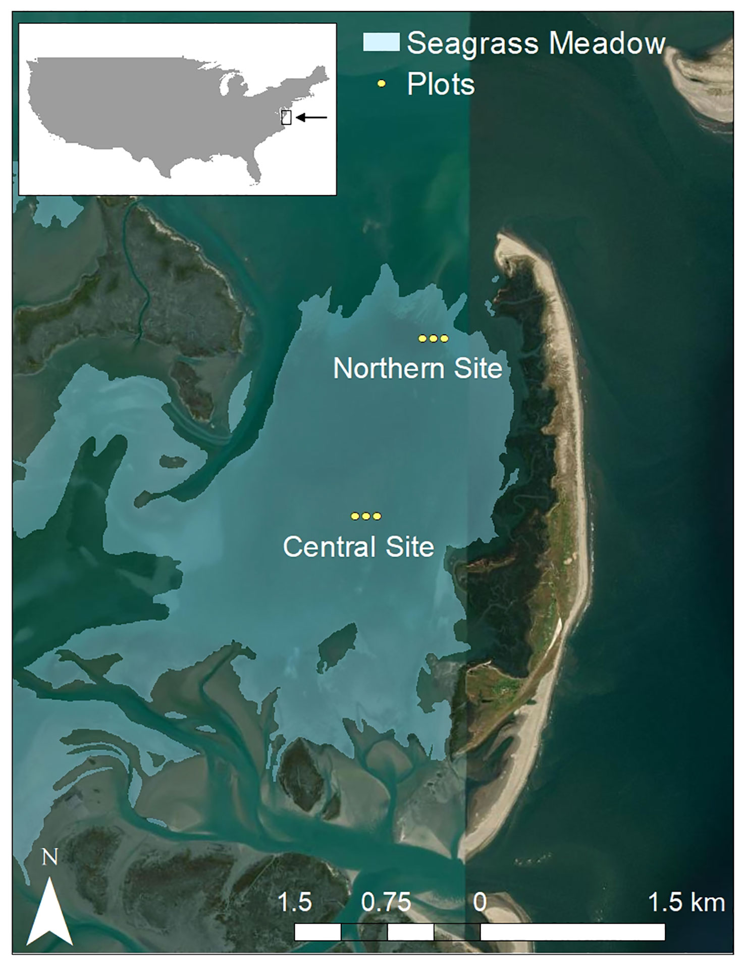
Figure 1 Location of plots containing subsurface sediment plates in South Bay seagrass meadow in the Virginia Coast Reserve Long-Term Ecological Research site. From left to right, plots 1C, 2C, and 3C are in the central site and plots 4C, 5C, and 6C are in the northern site. Spatial data credits: seagrass meadow coverage based on 2020 Chesapeake Bay SAV Coverage maps by the Virginia Institute of Marine Science (Orth et al., 2020); basemap credit Esri, DigitalGlobe, GeoEye, Earthstar Graphics, CNES/Airbus DS, USDA, USGS, AeroGRID, IGN, and the GIS User Community.

2.2 Study design

Subsurface sediment plates were deployed in replicates of three in each of six plots at the two sites within the meadow (Figure 1). At each site, three 3-m radius plots (~ 50 m apart) were marked with one tall PVC pipe in the center of the plot to identify the plot from above water, and delineated underwater with one small PVC pipe (extended ~ 10 cm above the sediment surface) at the plot edge in each cardinal direction. Within each plot, plates were deployed beneath the sediment (as described below) at 0.5 m, 1.5 m, and 2.5 m from the western edge of the plot along a transect that extended from the center of the plot to due west. Installing the plates uniformly along the same cardinal direction in each plot ensured that care was taken to avoid trampling near the plates in each plot. Plates were named based on their combined plot number and distance from the plot edge (e.g., 1C-0.5 is the plate 0.5 m from the edge in plot 1C).

2.3 Subsurface sediment plate deployment and measurements

Subsurface sediment plates were deployed on 5th of June 2020 via wading at low tide and using manual sediment coring techniques (Figure 2). Each plate was an 8.25 cm diameter, ~ 0.25 cm thick circular vinyl disk. To deploy the plate in the sediment, an 8.9 cm diameter, 30 cm length clear acrylic pipe that had been sanded to have a sharp cutting edge was hammered ~ 20 cm straight down into the sediment, plugged at the top with a rubber stopper, and removed, taking care to cover the bottom end of the tube to keep the sediment plug intact once removed. Simultaneously, a second person quickly inserted the plate into the bottom of the hole where the plug was removed and pushed it flat, and the sediment plug was carefully replaced into the hole on top of the plate, then the acrylic tube removed.

FIGURE 2

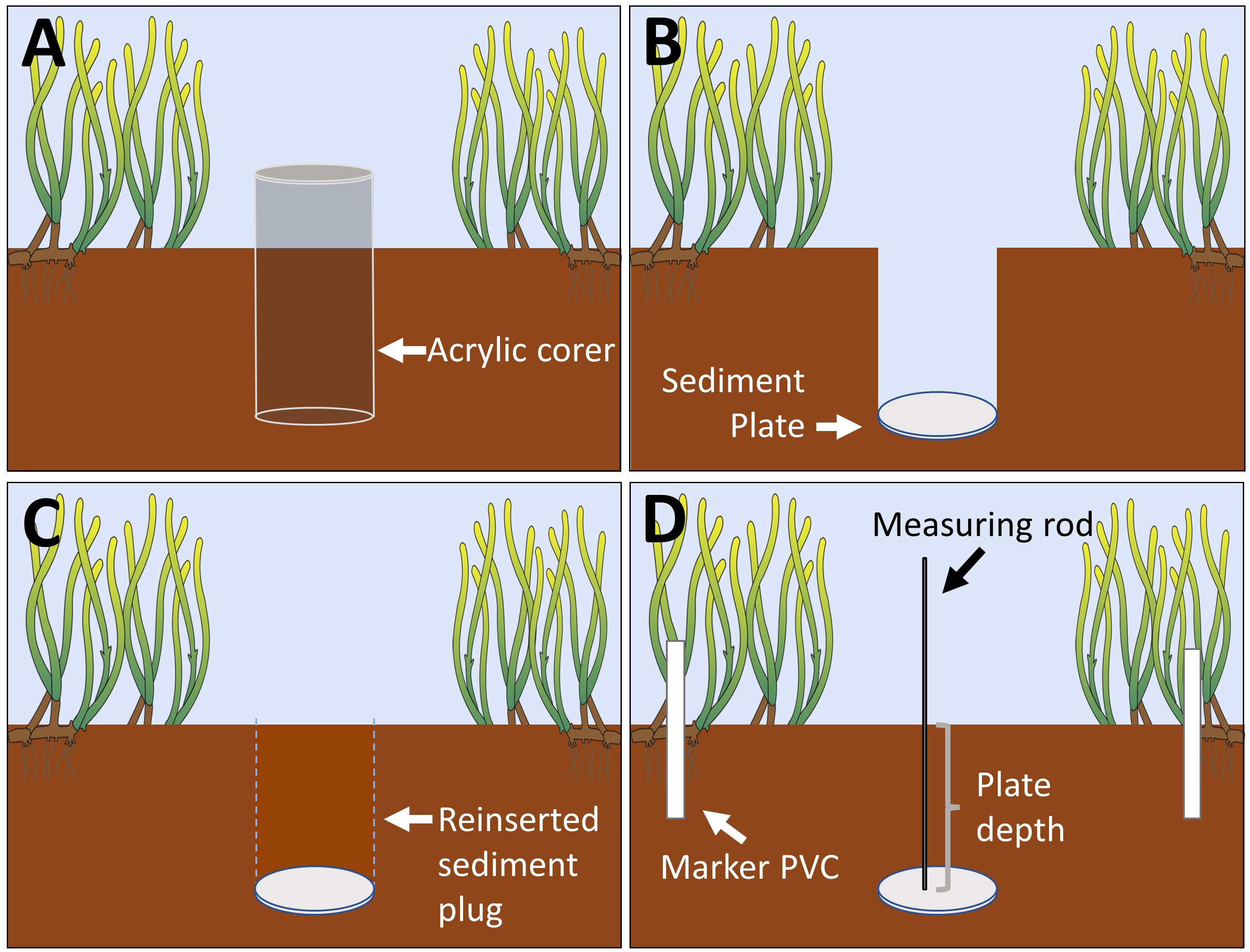
Figure 2 Subsurface sediment plate deployment and measurements. An acrylic core was hammered down into the sediment to remove a sediment plug (A), a sediment plate was placed at the bottom of the hole where the plug was removed (B), the sediment plug was reinserted into the hole above the plate (C), and sediment plate depth was measured using a thin metal rod to determine the height of the sediment horizon between the plate and the sediment surface (D). Mean sediment plate depth at the time of deployment was 14.8 cm ± SEM 1.1 cm. Seagrass image credit: Integration and Application Network (IAN), University of Maryland Center for Environmental Science, Cambridge, Maryland.

Plates were buried in the sediment, with a target depth of ~ 20 cm, for three reasons: 1) to allow for the measurement of the erosion of the sediment, rather than the accretion of the sediment alone; 2) to ensure that the plates were below the rhizosphere (that extends ~ 5-10 cm below the surface) which allowed them to stay in place regardless of sediment dynamics, season, or time frame of monitoring; and 3) to be shallow enough to be deployed by hand.

Initial plate depths were recorded (as described below) as a reference for deployment depth. To avoid errors associated with resuspension of sediments caused by plate deployment, the plate depth measurements recorded two weeks after deployment were used as the starting depth (T₀ depth) for later estimates of accretion and erosion. In the spring of 2021, small PVC pipe markers ~0.5 m away on either side (N and S) of each plate were installed to facilitate locating the plates. This approach was used to avoid manipulations near the sediment surface (associated with the use of sediment pins) that could otherwise impact accretion and erosion of the sediment surrounding the subsurface sediment plate.

Subsurface sediment plate depths were measured by inserting a thin (~2 mm) metal rod straight into the sediment until it hit the plate, marking the point of the sediment surface on the rod, and measuring the length of the rod between the end that touched the plate and the sediment surface. This was done three times for each sediment plate. The successful collection of three replicate measurements ensured that the substance hit by the rod was indeed the plate, as interference of the rod with a shell or other hard substance resulted in only one to two adjacent measurements since the interfering objects were not as wide as the plates. Measurements taken for objects mistaken for the plate were thrown out and prodding continued until the plate was successfully located and three replicate measurements were recorded. To further ensure no interfering objects were mistaken for plates, we removed suspicious outliers, as described below. The depth of the plate for each timepoint was calculated as an average of the three measurements to ensure that subtle differences in individual measurements caused by microtopography of the sediment surface and levelness of the plate were accounted for. Concurrently at five of the time points (T₀, 5 months, 11 months, 15 months, and 25 months), replicates of three (one at 11 months due to inclement weather) 4-cm diameter, 20-cm deep PVC sediment cores were collected in each plot (at 0.5, 1.5, and 2.5 m from the plot edge, on a transect away from the sediment plates) to determine if changes in belowground biomass drove changes in relative depth.

Plate depths were measured twelve times over the course of 25 months, focusing on the summer months when seagrasses were in their peak growing season and the weather was amenable for safely accessing sites. Plate depths were measured over one to three days, depending on site access. In addition to the initial measurements at the time of deployment (T_D), plate depths were measured twelve times after deployment at two weeks (T_D), one month, three months, five months, 11-16 months, 23 months, and 25 months (Table S1).

2.4 Data analysis

2.4.1 Data cleaning and processing

All data cleaning and analysis were done in R (R Core Team, 2022) and R Studio (Posit team, 2023), based primarily on the tidyverse package (Wickham et al., 2019). Replicate measurements for each plate were plotted by time and visually assessed for outliers based on the deviation from the other replicates at a single timepoint and measurements at adjacent timepoints. The three replicate measurements of each plate at each timepoint were averaged to reduce the inclusion of artifacts in individual plate measurements potentially introduced by microtopography of the sediment above the plates and levelness of the buried plate. Raw (true) depth values were used when calculating variability among replicates for a single plate at a single time point, while relative depth values were used for all analysis from the plate level up. Relative depths were calculated as the depth at a particular timepoint minus the original T₀ depth (two weeks after deployment), which was then set to zero as the baseline. Deployment depths (T_D) were not used as the baseline to reduce artifacts resulting from sediment resuspension and resettling during and after plate deployment.

2.4.2 Variability

Variability in plate measurements were calculated at three levels: variability in replicate measurements of a single plate at a single time point (within-plate variability), variability in average plate measurements at a single timepoint within a single plot (within-plot variability), and variability in average plot measurements at a single timepoint within a single site within the meadow (within-site variability). Within-plate variability was calculated based on raw depths by subtracting median depth from maximum depth and minimum depth from median depth for each set of plate replicates at a single timepoint, then averaging these two values to get a mean variability value for the plate at that timepoint, then averaging variability values across all plates at all timepoints. All standard errors were calculated using the “std.error” function from the plotrix package (Lemon, 2006). Within-plot variability was calculated based on the averages of three replicate plate measurements (which resulted in one depth value per plate per timepoint). Relative depth for each plate was calculated by subtracting the depth at each timepoint from the starting depth at T₀; the depth at T₀ was then set to zero as a baseline. Median depth was subtracted from maximum depth and minimum depth from median depth for each set of mean plate measurements within a plot at a single timepoint, then averaging these two values to get a mean variability value for the plot at that timepoint, then averaging variability values across all plots at all timepoints. Similarly, within-site variability was calculated by pooling the nine plates within each site at each time point, then calculating the average of all variability values across all timepoints. Across-site variability was calculated by pooling the 18 plates from across the two sites, then calculating the average of all variability values across all timepoints.

2.4.3 Sediment depths through time

A two-way repeated measures ANOVA was run to compare mean relative plate depths between sites and months, and to test for an interaction effect of the two. Two-sample t-tests were performed to compare sediment plate depths in the northern and central sites at each time point, following Fligner-Killeen tests of homogeneity of variances, which were used to inform the specifications of the t-test (i.e., whether there were equal variances).

2.4.4 Accretion rates

Accretion rates for each individual plate were estimated by fitting linear regressions to relative depth measurements over time, for both 0 to 13 and 0 to 25 month periods (June 2020 through July 2021 and June 2020 through July 2022, respectively; hereafter referred to as the 13-month and 25-month periods), and generating a slope, then converting the slope to cm yr^-1. A separate linear regression was run to test the correlation between accretion rate (based on 0-25 months) and deployment depth of each plate. To determine whether plots within a site differed in accretion rates, nested ANOVAs were run on accretion rates of individual plates (generated as described above) with site and plot number (nested by site) as predictors. Accretion rates for each site were estimated using linear regression on pooled plate depths within a site over all time points between 0-13 and 0-25 months, resulting in four estimated annual accretion rates.

3 Results

A total of 706 measurements were recorded for the plates following deployment. Prior to analysis, data from one plate (6C-1.5) were omitted from the dataset due to inconsistencies resulting from difficulties relocating the plate. Removal of 6 outliers (<1% of measurements) resulted in 664 measurements used in the analysis. Averaging replicate measurements for each plate at each timepoint resulted in 217 averaged measurements. Plates were deployed at a mean depth of 14.8 ± 1.1 cm ( ± SEM; n=14). Contributions of belowground biomass to total dry weight were negligible in relation to changes in relative plate depth.

3.1 Plate measurement variability

Mean variability in plate measurements across the three levels assessed ranged from 0.3 to 2.9 cm. Mean within-plate variability was 0.3 cm (± < 0.1 cm SEM; e.g., Figure S1). Mean within-plot variability was 1.3 ± 0.1 cm. Within-site variability was 2.9 ± 0.3 cm in the northern site and 2.0 ± 0.3 cm in the central site.

3.2 Trends in accretion and erosion across time at each site

Plate depths differed significantly by site (F_{1, 179} = 28.58, p=<0.0001), time (F_{11, 179} = 5.88, p=<0.0001), and the interaction of the site with time (F_{11, 179} = 4.29, p=<0.0001; Figure 3). There was no significant difference in relative plate depths between northern and central sites at 1, 3, 5, or 11 months (p>0.05 for two sample t-tests). At 13 months, there was significantly more sediment accreted in the northern compared to central site (3.9 and 1.6 cm, respectively; t(15)=-2.51, p=0.02), then plate depths were again no different at 14 and 15 months. At 16 months, sediment depth was marginally significantly higher in the northern compared to central site (3.8 and 2.0 cm, respectively; t(15)=-2.11, p=0.05). Sediment depths between sites continued to diverge in 2022, with northern sites having accumulated 3.8 cm total after 23 months compared to 0.1 cm in the central sites (t(15)=-5.53, p<0.0001), then 5.1 cm in the northern sites compared to 0.2 cm in the central sites after 25 months (t(15)=-6.81, p<0.0001, Figure S2).

FIGURE 3

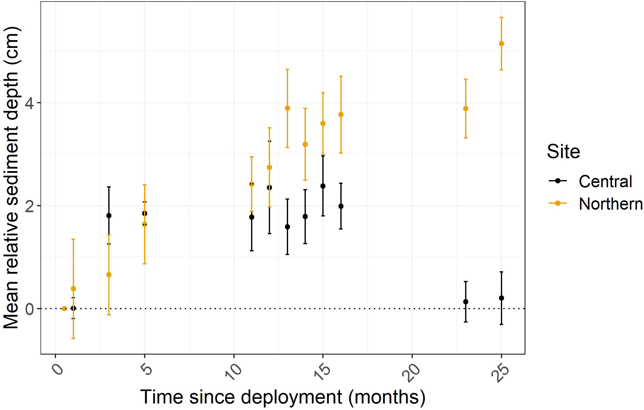
Figure 3 Mean relative sediment depth (cm) over time (months after plate deployment). Sediment depths have been normalized so that the T₀ depth is represented as the baseline (zero) and measurements thereafter are the result of subtracting the T₀ depth from the plate depth at T_x then pooling them for each site at each timepoint (per timepoint, Central n = 9 and Northern n = 8). Values above the dashed line on the y axis represent a gain in sediment compared to starting depths.

3.3 Sediment accretion rates

Twenty-five-month net accretion rates of plates were significantly different by site (two-way nested ANOVA, F_1,11 = 48.76, p<0.0001), but not by plot. Therefore, we pooled relative depth values of plates within each site to estimate a net annual accretion rate at each site (based on linear regression; Figures 4, 5; Table 1). There was no relationship between deployment depth and 25-month accretion rates of individual plates (F_1,29 = 0.13, p=0.73, Adj R²=-0.03; Figure S3).

FIGURE 4

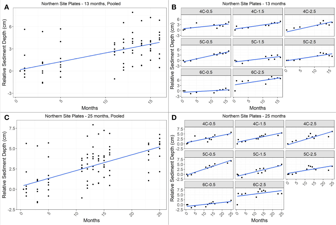
Figure 4 Linear regression of change in depth over time in the northern site for 13 months (top panels, A, B) and 25 months (bottom panels, C, D). Left panels (A, C) show the net change in relative sediment depth over time based on all pooled plate data for the site (n = 8 per timepoint); right panels (B, D) show change in sediment depth over time for individual plates. Annual accretion rate was 2.9 cm yr^-1 for the 13-month period (Adj R² = 0.33, F_1,78 = 40.46, p<0.0001) and 2.3 cm yr^-1 for the 25-month period (Adj R² = 0.38, F_1,94 = 59.89, p<0.0001).

FIGURE 5

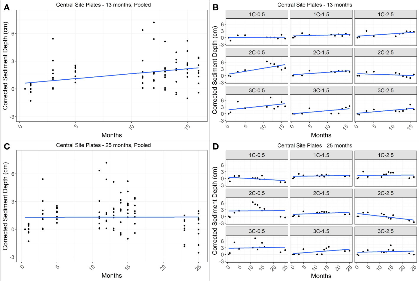
Figure 5 Linear regression of change in depth over time in the central site for 13 months (top panels, A, B) and 25 months (bottom panels, C, D). Left panels (A, C) show the net change in sediment depth over time based on all pooled plate data for the site (n=9 per timepoint); right panels (B, D) show change in sediment depth over time for individual plates. Annual accretion rate was 1.3 cm yr^-1 for the 13-month period (Adj R² = 0.13, F_1,87 = 13.96, p<0.001) and <0.1 cm yr^-1 for the 25-month period, which did not reflect a linear trend over time (Adj R²=-0.01, F_1,105<0.01, p=0.97).

TABLE 1

Table 1 Seagrass sediment accretion rates by method and location in the Virginia Coast Reserve.

In the northern site, relative sediment depth increased significantly over time, with net accretion rates of 2.9 cm yr^-1 based on the 13-month period (linear regression; Adj R² = 0.33, F_1,78 = 40.46, p<0.0001) and 2.3 cm yr-1 based on the 25-month period (linear regression; Adj R² = 0.38, F_1,94 = 59.89, p<0.0001; Figure 4). In the central site, relative sediment depth increased significantly over time for the 13-month period only, with a net accretion rate of 1.3 cm yr^-1 (linear regression; Adj R² = 0.13, F_1,87 = 13.96, p<0.001). Net accretion rate in the central site for the 25-month period was estimated to be <0.1 cm yr^-1, however, relative sediment depth did not have a linear relationship with time (linear regression; Adj R²=-0.01, F_1,105<0.01, p=0.97; Figure 5).

4 Discussion

In this study, we show how a novel, subsurface sediment plate method can be implemented for measuring relatively short-term changes (months to years) in seagrass surface sediment dynamics. Our results suggest that the method, which is cost-effective and easy to replicate, can successfully be used to understand loss and accumulation of sediments in seagrass meadows, and is practical and precise enough to be used across spatial scales in meadows. Here, we discuss spatial and temporal trends in sediment dynamics over a 25-month period, the sediment accretion rates estimated using the subsurface sediment plate method compared to previous estimates based on ²¹⁰Pb dating, the precision of the method, and our recommendations for implementing the method for measuring surface sediment dynamics in other seagrass settings.

4.1 Trends in sediment dynamics

Seagrass meadows are well known for their ability to slow water flow and encourage the settlement of particles to the seafloor, thereby continuously accreting new layers of sediment and burying previous layers. This process drives their ability to lock away organic carbon in an anaerobic environment where microbial remineralization is slow. However, this is an idealized model for seagrass functioning and the process of sedimentation can be much more dynamic.

In our study, we observed a relatively steady accumulation of sediments in the northern site, while in the central site we observed both accretion and erosion over the 25-month period. From 2020 to 2021, both the central and northern sites had a trend of accretion; however, the rate of accretion and amount of sediment accumulated in the northern site was higher than that of the central site. This difference in sediment burial between the northern and central sites can likely be attributed to the influence of hydrodynamics and position within the meadow. At the northern site, the seagrass is closer to the meadow edge, as well as the inlet, where flow velocity is higher (Safak et al., 2015). Being closer to the edge, the seagrasses at the northern site are among the first to slow water flowing into the seagrass meadow, resulting in deposits of larger grain size particles with lower organic carbon content at the northern edge compared to the central portion of the meadow (Oreska et al., 2017a). At the central site, seagrasses are buffered by the meadow, as well as the barrier island, resulting in slower water flow with smaller suspended particles remaining in the water column, as larger ones have already settled out as the water passed over the seagrass to reach the central portion of the meadow (Safak et al., 2015; Oreska et al., 2017a).

In 2022, plate measurements revealed a divergence between trends in the northern and central sites. In the northern site, surface elevation remained relatively constant between the fall of 2021 and spring of 2022, then increased in summer 2022, as expected (Figure 3). Although we were not able to take measurements in the wintertime (due to dangerous field conditions) to quantitatively show seasonal trends in sediment dynamics associated with winter, seagrasses in the VCR slough off their leaves in the autumn, which can trigger erosion of the sediments between autumn and spring if seagrass shoot density falls beneath 160-200 shoots m^-2 (Zhu et al., 2022). In the spring, seagrass growth increases, both from vegetative growth from remaining rhizomes and recruitment of new seedlings (Orth et al., 2020), resulting in the return of shoot densities high enough to enable sedimentation. In late June or early July, seagrasses reach their peak shoot density in the VCR (Berger et al., 2020), which is reflected in the northern site by the increase in surface elevation July 2022. In the central site, however, surface elevation decreased from fall 2021 to spring 2022 by about 2 cm and did not increase in summer 2022 (Figure 3). This reduction in surface elevation was likely the result of a disturbance, such as a storm. Although the northern site had not eroded between the final fall sampling of 2021 and the spring sampling of 2022, the relative sediment depth was approximately equal between the two timepoints, reflecting a net lack of accretion between the two sampling points. It is likely that the northern site was impacted by the same disturbance event (e.g., storm) as the central site in the winter or early spring of 2022; however, the generally higher shoot density in the northern site (e.g. summer 2021 northern = 553.6 ± 8.0 shoots m^-2 compared to central = 526.0 ± 8.5 shoots m^-2 (mean ± SEM) McGlathery, 2021) may have buffered the site from erosion, or the faster accretion rate in the northern site may have enabled it to recover any depth that was lost prior to the spring 2022 sampling.

Understanding seagrass response to sea level rise requires measurements of both sediment accretion rates and processes that influence shallow subsidence, including underground biomass and decay, compaction, and density, that determine overall surface elevation (Thomas and Ridd, 2004). Recently, seagrass scientists have adapted methods from other blue carbon ecosystems (salt marshes and mangrove forests) to improve our ability to track changes in seagrass surface elevation. Potouroglou et al. (2017) modified the RSET method (rod surface elevation tables) to create the SECP (Surface Elevation Change Pins) method, paired with marker horizons, to concurrently measure changes in surface elevation resulting from deeper (e.g., subsidence) and surface-level (e.g., accretion) processes. However, they faced challenges with creating horizon markers that could withstand the flow associated with tidal exchange in the intertidal and subtidal environment of seagrass meadows, and therefore could not measure contributions of sediment accretion to changes in surface elevation. The subsurface sediment plate method described in this study can replace traditional horizon marker methods in submerged ecosystems, and unlike traditional markers, can be used to quantify erosion in addition to accretion and is non-destructive. As such, this method can be used to make time-series measurements that can quantify the impact of discrete events on sediment erosion and accretion.

4.2 Subsurface sediment plate accretion rates vs. ²¹⁰Pb accretion rates

In this study, we used the subsurface sediment plate method to produce sediment accretion rates comparable to those produced by ²¹⁰Pb dating. ²¹⁰Pb dating is the most widely accepted method for estimating long-term sediment accretion rates in seagrass meadows (Potouroglou et al., 2017). Because these two methods represent sediment dynamics over very different time scales (months to years for sediment plates and up to 100 years for ²¹⁰Pb), a comparison of the two can provide insight into how short- and long-term sediment dynamics differ. Previous studies in the VCR LTER have used ²¹⁰Pb dating to estimate sediment accretion rates in South Bay meadow. The net accretion rate calculated in the present study for the central site based on the 13-month period was about twice that of the previous estimates for the central region of South Bay that used ²¹⁰Pb dating (1.3 cm yr^-1 in this study, compared to 0.6-0.7 cm yr^-1 in Oreska et al., 2017b and Greiner et al., 2013; Table 1). However, when accretion rate was estimated for the entire 25-month period of our study, the net accumulation rate at the central site was negligible (<0.1 cm yr^-1) due to an erosion event prior to the spring and summer 2022 sampling. Accretion in the northern site was much more consistent than in the central site, resulting in higher annual accretion rates for both the 13- and 25-month periods (2.9 and 2.3 cm yr^-1, respectively; Table 1). The lower accretion rate for the 25-month period at the northern site compared to the 13-month is a reflection of the impact of the disturbance that caused erosion in the central site. These results suggest that the sediment plate method successfully captured short-term sediment dynamics, including shifts between accreting and erosive states, that determine long-term net rates of sediment accretion.

From this study, we see that the minimum time period necessary to confidently derive accretion rates using the subsurface sediment plate method is site-dependent and may vary based on stochastic events. Depth measurements collected infrequently or analyzed in isolation provide only a snapshot of sediment depths and may lead to over- or underestimates of net accretion rates (e.g., Figure S2). Previous estimates of accretion rates in South Bay meadow using ²¹⁰Pb were based on the top 10-11 cm of sediment, reflecting net accretion rates over the 10-14 years since seagrass restoration, plus years prior at the deepest end of the dated core. In comparison, the subsurface sediment plate method used here has the benefit of capturing individual sedimentation and erosion events that occur in response to environmental forcings over months to years. The subsurface sediment plate method can be applied to newly restored seagrass meadows, unlike the ²¹⁰Pb method, which has proven unsuccessful in bare sediment or recently restored meadows (<10 y), which can take around a decade to reach functional equivalence in shoot density and sediment accretion rate (McGlathery et al., 2012; Table 1). However, caution must be used to avoid misinterpreting short-term events as representations of long-term net trends in sediment accumulation. Due to the varying sediment dynamics observed over time and space in our study, we suggest that subsurface sediment plates deployed for the purpose of producing net accretion rates be monitored for longer time periods (i.e., years) at frequent intervals (monthly to bi-monthly). These rates will be useful for estimating accretion rates and carbon additionality for newly restored meadows; still, additional comparisons and controlled experiments are recommended to further our understanding of the physical and biological processes that influence real-time and retrospective measurements of sedimentation rates, and how environmental processes driving sedimentation rates differ over months to centuries.

4.3 Variability across replicates and space

Subsurface sediment plate measurements were very consistent within replicates of a single plate (within-plate variability = 0.3 cm ± <0.1 cm) and variability in measurements increased with spatial distance, as expected (within-plot variability = 1.3 ± 0.1 cm; within-site variability = 2.9 ± .03 cm). The low variability in replicate plate measurements demonstrates that this method is precise enough to pick up on very small changes in the sediment surface. The ability to detect small changes in seagrass sediments over time is necessary for assessing how short-term or localized conditions influence accretion and erosion, thereby determining long-term patterns in net sediment accretion. As demonstrated here, small disturbances, such as storms, can punctuate an otherwise steadily accreting site with periods of erosion that interrupt the accumulation of sediments. The increase in variability from measurements of plates within a single plot to plates across plots within a site (and marked differences across sites) suggests that differences in sediment dynamics increase with distance within the meadow on the scale of tens to thousands of meters.

5 Conclusions and recommendations

We have demonstrated that the subsurface sediment plate method can be used to quantify changes in surface sediment dynamics spatially and temporally, over periods of months to years. Considering the variability we observed in surface sediment dynamics over time, and how these differed across spatial scales, we recommend that measurements used to calculate net accretion rates be conducted monthly to bi-monthly for multiple years, so that the role of seasonal trends and stochastic disturbances can be incorporated into long-term sediment accretion rates. In the short-term, subsurface sediment plates can be used to observe how particular events or phenomena impact sediment accretion and erosion, which can then be incorporated into our understanding of long-term sediment dynamics and accretion rate estimates. Here, we provide the following guidelines for reducing errors associated with the limitations of the method, by suggesting that plates be deployed:

1) In sediments without many hard substances (e.g., very shelly areas, such as at the edge of an oyster bed), as hard objects within the sediments can make initial installation and plate identification challenging, or lead to artificially shallower recorded depths if hard objects are mistaken for plates;

2) In sediments not prone to excessive compaction. Compaction of the core plug during deployment could alter the starting elevation, producing artifacts in accumulation measurements resulting from increased sedimentation within the depression caused sediment compaction above the plate;

3) In sediments not prone to excessive bioturbation. Minimal amounts of bioturbation by small organisms is unlikely to have substantial impacts on the functionality of the method (i.e., the plate is likely to stay in place), but may alter surface elevation. Larger burrowing organisms and grazing megafauna, on the other hand, may have the potential to unearth the subsurface plates;

4) For a period of months to years. Very short-term measurements (e.g., days) may be misleading. The high resuspension and deposition dynamics in most seagrass meadows lead to variable plate measurements over the short term, therefore longer monitoring periods are required to see broad patterns (i.e., get beyond the “noise” of measurement variability and natural seasonal/short-term variability); measurements across months may be sufficient for understanding short-term sedimentary processes, while year time scales are necessary to estimate net accumulation rates that incorporate stochastic sediment gains and losses;

5) At depths appropriate for the local seagrass species and potential disturbances. In our study, an average deployment depth of ~15 cm was appropriate for ensuring plates were below the rhizosphere, which extends ~5-10 cm deep at our site for Z. marina. However, we suggest deployment of the plates at greater depths for species with extensive rhizospheres (e.g., Posidonia species) or in sites that are prone to experiencing extreme erosive events that may impact sediments deeper than the rhizosphere (i.e., with seagrass loss); additionally, we suggest plates be buried deep enough to capture the maximum expected erosion depths based on local disturbance types;

6) With concurrent measurements of belowground biomass. Changes to belowground biomass may impact surface elevation; this method alone does not distinguish between belowground growth/decay and sediment accretion/erosion. Discrepancies in sediment depths caused by changes in belowground biomass (or lack thereof, as in this study) may be identified by taking concurrent cores nearby (e.g., ~ 1 m away) at each timepoint to determine if changes in belowground biomass correlate with changes in sediment depth;

7) (optionally) With a double lined corer and leveler. In our study, extrusion of sediment cores using a single corer was sufficient for burying plates beneath the rhizosphere (~15 cm deep). However, in some sediments, the hole may collapse after removing the sediment plug, making it difficult to deploy plates to the desired depth. To avoid this, we recommend a double lined corer be used in which the outer liner can stay in place to hold the sediment hole open, while the inner liner is used to remove the sediment plug. Use of a double lined corer can also help ensure that sediment plates are perfectly level at deployment; once the plate is placed at the bottom of the hole, an extra empty core liner can be placed on top, within the outer liner, on top of the plate, with a leveler placed on top of the inner liner. The plate can be adjusted until the leveler on top of the inner core indicates the plate is level. Then, the extra inner liner and leveler can be removed, the inner liner with the sediment plug can be replaced, and both the inner and outer core liners can be removed with the plate and sediment in place.

8) (optionally) With concurrent measurement of sediment organic carbon. Carbon stocks are easy to measure with sediment coring and can be used in conjunction with plate measurements to quantify carbon sequestration rates. Concurrent measurements nearby (~ 1 m away) can improve our understanding of real-time carbon gains and losses associated with sediment dynamics in seagrass meadows that contribute to net sequestration rates. Application of this method to seagrass blue carbon projects may provide a more reliable method of calculating additionality compared to traditionally used ²¹⁰Pb methods.

We conclude that the subsurface sediment plate method is a useful tool for quantifying changes in seagrass sediment accumulation and erosion over time and space. Future studies to validate the method, for example, with concomitant measurements of accretion using alternative methods and pairing it with methods measuring deeper sedimentological processes, will be valuable for improving our understanding of both the ecological and methodological factors that determine sediment accretion rates as calculated with the present method. Employing this method in seagrass meadows can, for minimal cost and effort, improve our understanding of sediment dynamics in seagrass meadows, carbon sequestration and additionality in blue carbon projects, and the impacts of disturbance and recovery on seagrass functioning and ecosystem services. Additionally, this method can be paired with existing methods to assess the ability of seagrass meadows to keep pace with sea level rise.

Data availability statement

The original contributions presented in the study are included in the article/Supplementary Material. Further inquiries can be directed to the corresponding author.

Author contributions

CL and KM conceived and designed the study. CL designed the method with feedback from KM. CL collected and analyzed the data. CL wrote the first draft of the manuscript. All authors contributed to the article and approved the submitted version.

Funding

This work was supported by the National Science Foundation via the Virginia Coast Reserve Long Term Ecological Research project (DEB-1832221) and by the University of Virginia’s Environmental Institute.

Acknowledgments

We thank the staff and students of the University of Virginia’s Coastal Research Center for logistical support and assistance with data collection, especially Katherine Webber, Kylor Kerns, Spencer Tassone, Cora Baird, Jonah Morreale, and David Lee.

Conflict of interest

The authors declare that the research was conducted in the absence of any commercial or financial relationships that could be construed as a potential conflict of interest.

Publisher’s note

All claims expressed in this article are solely those of the authors and do not necessarily represent those of their affiliated organizations, or those of the publisher, the editors and the reviewers. Any product that may be evaluated in this article, or claim that may be made by its manufacturer, is not guaranteed or endorsed by the publisher.

Supplementary material

The Supplementary Material for this article can be found online at: https://www.frontiersin.org/articles/10.3389/fmars.2023.1232619/full#supplementary-material

References

Alemu I J. B., Puah J. Y., Friess D. A. (2022). Shallow surface elevation changes in two tropical seagrass meadows. Estuar. Coast. Shelf Sci. 273, 107875. doi: 10.1016/j.ecss.2022.107875

CrossRef Full Text | Google Scholar

Aoki L. R., McGlathery K. J., Wiberg P. L., Al-Haj A. (2020). Depth affects seagrass restoration success and resilience to marine heat wave disturbance. Estuaries Coasts. 43, 316–328. doi: 10.1007/s12237-019-00685-0

CrossRef Full Text | Google Scholar

Arias-Ortiz A., Masqué P., Garcia-Orellana J., Serrano O., Mazarrasa I., Marbà N., et al. (2018). Reviews and syntheses: 210Pb-derived sediment carbon accumulation rates in vegetated coastal ecosystems - setting the record straight. Biogeosciences 15, 6791–6818. doi: 10.5194/bg-15-6791-2018

CrossRef Full Text | Google Scholar

Berger A. C., Berg P., McGlathery K. J., Delgard M. L. (2020). Long-term trends and resilience of seagrass metabolism: A decadal aquatic eddy covariance study. Limnol. Oceanogr. 65, 1423–1438. doi: 10.1002/lno.11397

CrossRef Full Text | Google Scholar

Carnell P. E., Ierodiaconou D., Atwood T. B., Macreadie P. I. (2020). Overgrazing of seagrass by sea urchins diminishes blue carbon stocks. Ecosystems 23, 1437–1448. doi: 10.1007/s10021-020-00479-7

CrossRef Full Text | Google Scholar

Cullen-Unsworth L., Unsworth R. (2013). Seagrass meadows, ecosystem services, and sustainability. Environment 55, 14–28. doi: 10.1080/00139157.2013.785864

CrossRef Full Text | Google Scholar

de Boer W. F. (2007). Seagrass-sediment interactions, positive feedbacks and critical thresholds for occurrence: a review. Hydrobiologia 591, 5–24. doi: 10.1007/s10750-007-0780-9

CrossRef Full Text | Google Scholar

Ewers Lewis C. J., Baldock J. A., Hawke B., Gadd P. S., Zawadzki A., Heijnis H., et al. (2019). Impacts of land reclamation on tidal marsh ‘blue carbon’ stocks. Sci. Total Environ. 672, 427–437. doi: 10.1016/j.scitotenv.2019.03.345

PubMed Abstract | CrossRef Full Text | Google Scholar

Green E., Short F. T. (Eds.) (2003). World Atlas of seagrasses. (Berkeley, USA: University of California Press). doi: 10.5860/choice.41-3160

CrossRef Full Text | Google Scholar

Greiner J. T., McGlathery K. J., Gunnell J., McKee B. A. (2013). Seagrass restoration enhances “blue carbon” sequestration in coastal waters. PloS One 8, e72469. doi: 10.1371/journal.pone.0072469

PubMed Abstract | CrossRef Full Text | Google Scholar

Lafratta A., Serrano O., Masqué P., Mateo M. A., Fernandes M., Gaylard S., et al. (2020). Challenges to select suitable habitats and demonstrate ‘additionality’ in Blue Carbon projects: A seagrass case study. Ocean Coast. Manage. 197, 105295. doi: 10.1016/j.ocecoaman.2020.105295

CrossRef Full Text | Google Scholar

Lei J., Schaefer R., Colarusso P., Novak A., Simpson J. C., Masqué P., et al. (2023). Spatial heterogeneity in sediment and carbon accretion rates within a seagrass meadow correlated with the hydrodynamic intensity. Sci. Total Environ. 854, 158685. doi: 10.1016/j.scitotenv.2022.158685

CrossRef Full Text | Google Scholar

Lemon J. (2006). Plotrix: a package in the red light district of R. R-News 6 (4), 8–12.

Google Scholar

Macreadie P. I., Trevathan-Tackett S. M., Skilbeck C. G., Sanderman J., Curlevski N., Jacobsen G., et al. (2015). Losses and recovery of organic carbon from a seagrass ecosystem following disturbance. Proc. R. Soc B 282, 20151537. doi: 10.1098/rspb.2015.1537

CrossRef Full Text | Google Scholar

Macreadie P. I., York P. H., Sherman C. D. H., Keough M. J., Ross D. J., Ricart A. M., et al. (2014). No detectable impact of small-scale disturbances on “blue carbon” within seagrass beds. Mar. Biol. 161, 2939–2944. doi: 10.1007/s00227-014-2558-8

CrossRef Full Text | Google Scholar

Marbà N., Arias-Ortiz A., Masqué P., Kendrick G. A., Mazarrasa I., Bastyan G. R., et al. (2015). Impact of seagrass loss and subsequent revegetation on carbon sequestration and stocks. J. Ecol. 103, 296–302. doi: 10.1111/1365-2745.12370

CrossRef Full Text | Google Scholar

McGlathery K. J. (2021). Density of Seagrass in Virginia Coastal Bays, 2007-2021 ver 19. Environmental Data Initiative. doi: 10.6073/pasta/74ac4c8d78f89935e4a77a8f310c9ac4 (Accessed 2023-09-12).

CrossRef Full Text | Google Scholar

McGlathery K. J., Reynolds L. K., Cole L. W., Orth R. J., Marion S. R., Schwarzschild A. (2012). Recovery trajectories during state change from bare sediment to eelgrass dominance. Mar. Ecol. Prog. Ser. 448, 209–221. doi: 10.3354/meps09574

CrossRef Full Text | Google Scholar

Oreska M. P. J., McGlathery K. J., Porter J. H., Bost M., McKee B. A. (2017a). Seagrass blue carbon accumulation at the meadow-scale. PloS One 12, 1–18. doi: 10.1371/journal.pone.0176630

CrossRef Full Text | Google Scholar

Oreska M. P. J., Wilkinson G. M., McGlathery K. J., Bost M., McKee B. A. (2017b). Non-seagrass carbon contributions to seagrass sediment blue carbon. Limnol. Oceanogr. 63, S3–S18. doi: 10.1002/lno.10718

CrossRef Full Text | Google Scholar

Orth R. J., Lefcheck J. S., Mcglathery K. S., Aoki L., Luckenbach M. W., Moore K. A., et al. (2020). Restoration of seagrass habitat leads to rapid recovery of coastal ecosystem services. Sci. Adv. 6, 1–10. doi: 10.1126/sciadv.abc6434

CrossRef Full Text | Google Scholar

Orth R., McGlathery K. (2012). Eelgrass recovery in the coastal bays of the Virginia Coast Reserve, USA. Mar. Ecol. Prog. Ser. 448, 173–176. doi: 10.3354/meps09596

CrossRef Full Text | Google Scholar

Posit team (2023). RStudio: integrated development environment for R (Boston, MA: Posit Software, PBC).

Google Scholar

Potouroglou M., Bull J. C., Krauss K. W., Kennedy H. A., Fusi M., Daffonchio D., et al. (2017). Measuring the role of seagrasses in regulating sediment surface elevation. Sci. Rep. 7, 1–11. doi: 10.1038/s41598-017-12354-y

PubMed Abstract | CrossRef Full Text | Google Scholar

R Core Team (2022). R: A language and environment for statistical computing. R Foundation for Statistical Computing (Vienna, Austria).

Google Scholar

Safak I., Wiberg P. L., Richardson D. L., Kurum M. O. (2015). Controls on residence time and exchange in a system of shallow coastal bays. Cont. Shelf Res 97, 7–20. doi: 10.1016/j.csr.2015.01.009

CrossRef Full Text | Google Scholar

Thomas S., Ridd P. V. (2004). Review of methods to measure short time scale sediment accumulation. Mar. Geol. 207, 95–114. doi: 10.1016/j.margeo.2004.03.011

CrossRef Full Text | Google Scholar

Wickham H., Averick M., Bryan J., Chang W., McGowan L. D., François R., et al. (2019). Welcome to the tidyverse. J. Open Source Software 4 (43), 1686. doi: 10.21105/joss.01686

CrossRef Full Text | Google Scholar

Zhu Q., Wiberg P. L., McGlathery K. J. (2022). Seasonal growth and senescence of seagrass alters sediment accumulation rates and carbon burial in a coastal lagoon. Limnol. Oceanogr. 67, 1931–1942. doi: 10.1002/lno.12178

CrossRef Full Text | Google Scholar