Ocean mixing induced by three-dimensional structure of equatorial mode tropical instability waves in the Pacific Ocean

Observations have revealed that tropical instability waves (TIWs) play an important role in the ocean mixing of the equatorial thermocline. However, most studies have not distinguished the individual effects from the TIWs’ two modes, and most of them focused on the effect of the TIW-induced vertical shear on the formation of mixing. In this study, we utilize the high-resolution ocean reanalysis data to isolate the 3D structure of the equatorial mode of TIW (eTIW) and examine the detailed mechanisms of its mixing effects. Horizontally, the temperature associated with the eTIWs shows a centrosymmetric structure in the upper layers, but vertically, the phase begins to transition at ~70 and becomes opposite to that of the upper layer below 90 m. The centrosymmetric temperature structure leads to a similar stratification pattern in the upper layers. We find that the pattern of the eTIW-associated reduced shear squared (RSS), an indicator for potential shear instability, is controlled by its stratification rather than shear, suggesting that the former plays a more important role than the latter in resulting in shear instability and mixing. Specifically, it is in the northern (southern) part of the clockwise (anticlockwise) phase of the eTIWs that the eTIW-associated RSS is positively large, where the total flow is more likely to be modulated by shear instability and mixing. Hence, the present study provides a new mechanism for the TIW-induced mixing in the equatorial thermocline. However, in specific regions where the eTIW-induced shear has the same sign as that of the mean flow, the eTIW-associated shear squared can also significantly enhance the total RSS and lead to shear instability, consistent with previous studies.

1 Introduction

Tropical instability waves (TIWs) are westward propagating waves that occur in the cold tongue region of the tropical eastern Pacific and Atlantic Oceans. They have a distinct period of 12–40 days and wavelengths of ~1,000 km. The modal characteristics of the TIWs were not clearly identified until Lyman et al. (2007) identified dual TIW modes according to the observed temperature fluctuations. TIWs are divided into 17-day TIWs (Yanai wave-initiated) with a central period of ~17 days concentrated at the equator and 33-day TIWs (Rossby wave-initiated) with a central period of ~33 days concentrated north of the equator (at ~4°N). Liu et al. (2019a) constructed the horizontal flow structures of the two modes and referred to the 17-day TIWs as equatorial mode TIWs (eTIWs). Compared with an ideal Yanai wave, the eTIWs display an antisymmetric, trans-equatorial structure and a northeast-southwest (NE-SW)-inclined flow pattern near the equator. Whereas, the 33-day mode was manifested as a strong nonlinear vortex structure north of the equator (that is, tropical instability vortex, TIV; Flament et al., 1996; Liu et al., 2019a; hereafter vTIWs). Both the eTIW and vTIW show an obvious inclined structure, which partly reflects the barotropic instability of the equatorial flow.

TIWs are important mesoscale processes that play a critical role in the regional energy cascade. It has been observed that TIWs can connect surface cooling in the equatorial Pacific via small-scale turbulent mixing (Moum et al., 2009). Liu et al. (2016) found that shear instability and mixing occur more frequently in the thermocline during the TIW periods. Cherian et al. (2020) found widespread downward turbulent heat fluxes induced by TIWs in the thermocline. Whitt et al. (2021) reproduced TIW-induced strong turbulences through large eddy simulation (LES). Warner et al. (2018) identified two distinct small-scale fronts at the trailing edge of TIWs, which may give rise to gravity waves and impact the heat flux at the air–sea interface.

A question arises about how TIWs lead to mixing. Previous studies have mostly attributed it to TIW-associated vertical velocity shear. Moum et al. (2009) suggested that the shear resulting from the strong meridional component of TIWs’ velocity enhances mixing. Holmes and Thomas (2015), on the other hand, argued that the zonal component of velocity plays an important role. Liu et al. (2019a) isolated the eTIWs and vTIWs and identified the crucial role played by the TIWs’ zonal velocity component in inducing mixing via TIW–mean flow interaction. Liu et al. (2020) made further advancements in understanding the formation of a strongly turbulent layer in the upper thermocline (Moum et al., 2009; Inoue et al., 2012), which was found to result from the shear of a combination of various equatorial waves, including the TIWs.

Notably, Liu et al. (2020) discovered that the stratification fluctuations associated with these equatorial waves also have an important impact on the formation of mixing. The underlying mechanism is that equatorial waves are associated with shoaling and deepening along with different phases. However, Liu et al. (2020) focused solely on a single site (140°W) at the equator. In this study, we aim to comprehensively investigate the 3D structural characteristics of shear squared, stratification, and reduced shear squared (RSS) corresponding to the eTIWs using high-resolution reanalysis and examine their influences on the formation of turbulent mixing.

The reanalysis employed and analysis methods used in this study are introduced in Data and method. In the session The 3D structure of eTIWs, we present the 3D distribution of velocity and temperature for eTIWs. In the session Shear instability and mixing properties, we analyze the shear instability and mixing characteristics, including the stratification, the shear squared, and the RSS structure of eTIWs. Finally, we provide a summary and discuss the findings in Summary and discussion.

2 Data and method

2.1 Data

In this study, we utilize daily averaged temperature and velocity data from the HYbrid Coordinate Ocean Model (HYCOM) reanalysis to characterize the temperature, velocity, and mixing properties of eTIWs. The data have a horizontal resolution of 0.08° × 0.08° and a nonuniform vertical grid spacing. The average grid interval is 2 m above 15 m depth and 5 m between 15 m and 50 m, and 10 m, 25 m, and 50 m in intervals of 50–100 m, 100–150 m, and 150–300 m, respectively. The selected area for analysis is (130°–146°W, 6°S–6°N), and the time range spans from 1 January 2000 to 31 December 2001.

Furthermore, we incorporate daily sea surface temperature (SST) data from the Optimum Interpolation SST (OISST) dataset for the years 2008 to 2019. The SST data has a resolution of 0.25°×0.25° and is used to identify eTIWs in the region spanning (110°–150°W, 5°S–5°N).

2.2 Methods

2.2.1 Composition analysis of the 3-D structure of eTIWs

2.2.1.1 Identifying the eTIWs by their characteristic periods

In this study, we primarily employ the composition analysis method, with the detailed data processes described below. It should be noted that the characteristic period of eTIWs in the model data may differ from that in the actual observed data. To identify the specific periods and investigate the depth dependence of the eTIWs, we perform the power spectral density (PSD) analysis of the velocity components ($u$, $v$) for the upper 300 m. Since TIWs are particularly strong during the boreal fall to winter period, the PSD analysis is performed from 15 September 2000 to 15 January of the following year, coinciding with the period when strong eTIWs were observed (Liu et al., 2019a). According to the flow field diagram of eTIWs by Liu et al. (2019a), it is evident that the meridional component of the surface velocity of eTIWs at the equator is dominant. In addition, the northern boundary of its vortex extends roughly to 3°–4°N, displaying a pronounced zonal component in velocity therein. Therefore, we present the results of the PSD analysis at (136°W, 3.6°) and (136°W, 0°N), respectively (Figure 1). The analysis reveals several distinct characteristic periods associated with different types of fluctuations. Notably, the eTIWs exhibit a prominent characteristic period ranging from approximately 12–24 days, primarily concentrated from the sea surface to the upper layer of the ocean at about 120 m. The PSD analysis conducted at other latitudes within the cold tongue region yields similar results.

FIGURE 1

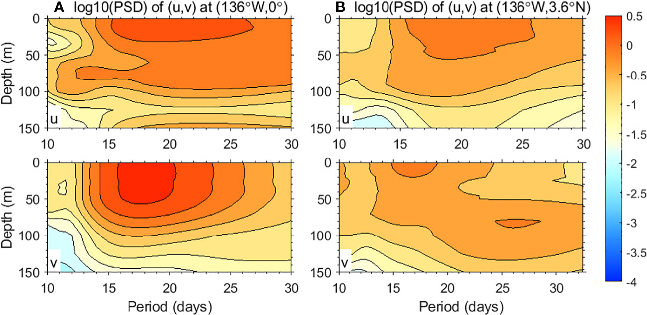
Figure 1 Results of PSD analysis of daily velocity with a 30-day high-pass filter at (A) (136°W, 0°) and (B) (136°W, 3.6°N) for the upper 150 m from December 2000 to January 2001, respectively, at a logarithmic scale. The Hanning window and step length are set to 60 and 10 days, respectively. The confidence level is 0.95.

2.2.1.2 Sampling the eTIWs

After the characteristic period is obtained, the eTIW-associated zonal and meridional velocity anomalies ($u^{\prime }$ and $v^{\prime }$), the temperature anomalies ($T^{\prime }$), the salinity anomalies ($S^{\prime }$), the density anomalies (${\rho }^{\prime }$) and other properties (see below) can be obtained by 12–24 days of band-pass filtering those properties over the cold tongue region (130°–150°W, 6°S–6°N). The Hovmöller diagram of $u^{\prime }$ at a typical depth of 40 m clearly illustrates the westward propagation and also implies the inclined flow pattern (NE-SW) of the eTIWs (Figure 2).

FIGURE 2

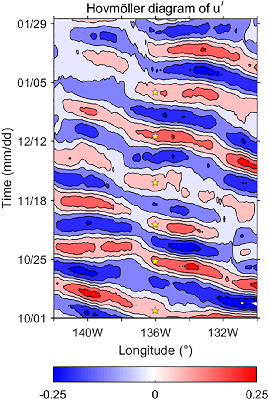
Figure 2 Hovmöller diagram of the 12–24-day band-pass filtered $u^{\prime }$ (unit: ms⁻¹) during October 2000 to January 2001 at 40 m depth along (130–142°W, 0°). The pentagram symbols represent the selected time for the characteristic eTIWs at 136°W.

To ensure an accurate and comprehensive representation of eTIWs and to enhance the generalizability of the results, we select three locations in the equatorial eastern Pacific: (136°W, 0°), (138°W, 0°), and (140°W, 0°). These locations are chosen to obtain a sufficient number of samples. The identification of eTIWs is determined based on the time when the eTIWs’ maximum $u^{\prime }$ at the equator at the 40-m depth passed the representative latitudes. Here, the reason we choose $u^{\prime }$ as the indicator, rather than $v^{\prime }$, is to highlight the inclined flow pattern of the eTIW. We found that no significant difference in the 3D structure of eTIW shows up between v’- and u’-based composites. Consequently, anomalous properties associated with eTIWs are documented within a 12° extension in both the zonal and meridional directions centered around the three locations, respectively. The selected characteristic times for (136°W, 0°) are 14 and 25 August, 12 September, 4 and 24 October, 8 and 25 November, and 14 December 2000 and 1 and 18 January 2001. For (138°W, 0°), the selected times are 28 August, 15 September, 8 and 30 October, 15 and 28 November, and 20 December 2000 and 12 January 2001. Lastly, for (140°W, 0°), the selected times are 11 August, 2 and 25 September, 11 and 30 October, 17 November, and 7 and 24 December 2000 and 16 January 2001. In total, there are 27 snapshot (daily) eTIW samples obtained, which all display obvious morphological characteristics of a (tilted) Yanai wave. It is worth mentioning that the samples are enough to construct a general eTIW with significance. We have observed that increasing the sample number does not alter the general properties of the eTIWs (not shown).

2.2.1.3 Compositing the eTIW with the samples

The zonal coordinate of the samples is rearranged to be −6° to 6°, with the zonal center of the eTIW (the longitude of maximum $u^{\prime }$) at 0°. The meridional coordinate is 6°S to 6°N. Subsequently, the eTIW-associated 3D velocity, temperature, and density fields are constructed (Figures 3–5). Additionally, the eTIW-corresponding 3D total velocity, temperature, salinity, density, the velocity shear squared, buoyancy frequency squared, the RSS, as well as the mean properties, respectively, are also constructed based on the samples (see below). The mean properties are obtained by applying a 45-day low-pass filter (Liu et al., 2019a; Liu et al., 2019b; Liu et al., 2020).

FIGURE 3

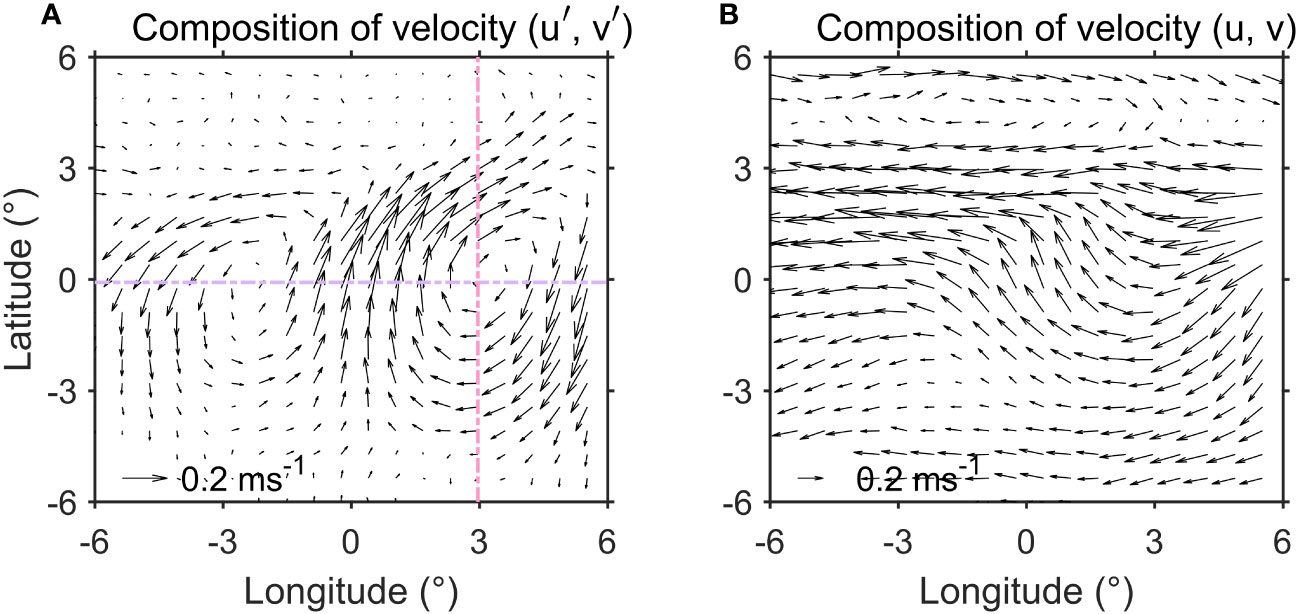
Figure 3 (A) The composite of eTIW-associated velocities ($u^{\prime }, v^{\text{'}}$) at 40 m, based on samples centered at (136°W, 0°), (138°W, 0°), and (140°W, 0°). (B) The composite total flow field ($u, v$) corresponding to the eTIWs in (A) (unit: ms⁻¹). The pink and purple dotted lines represent the latitudinal and longitudinal sections that are used for the representation of the sectional structure of the eTIWs in Figure 4.

FIGURE 4

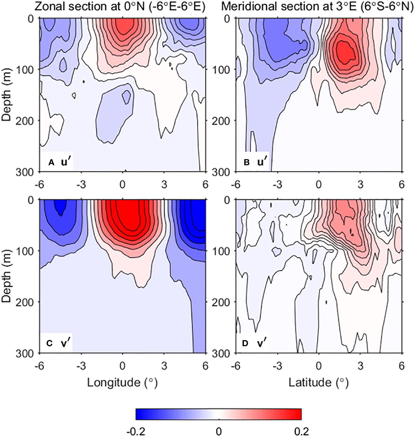
Figure 4 The composite of eTIW-associated velocity ($u^{\prime }, v^{\text{'}}$) along two sections: (A, C) the zonal section at equator and (B, D) the meridional section crossing the center of the clockwise part of the eTIWs, with the location of the sections being denoted in Figure 3 (unit: ms⁻¹).

FIGURE 5

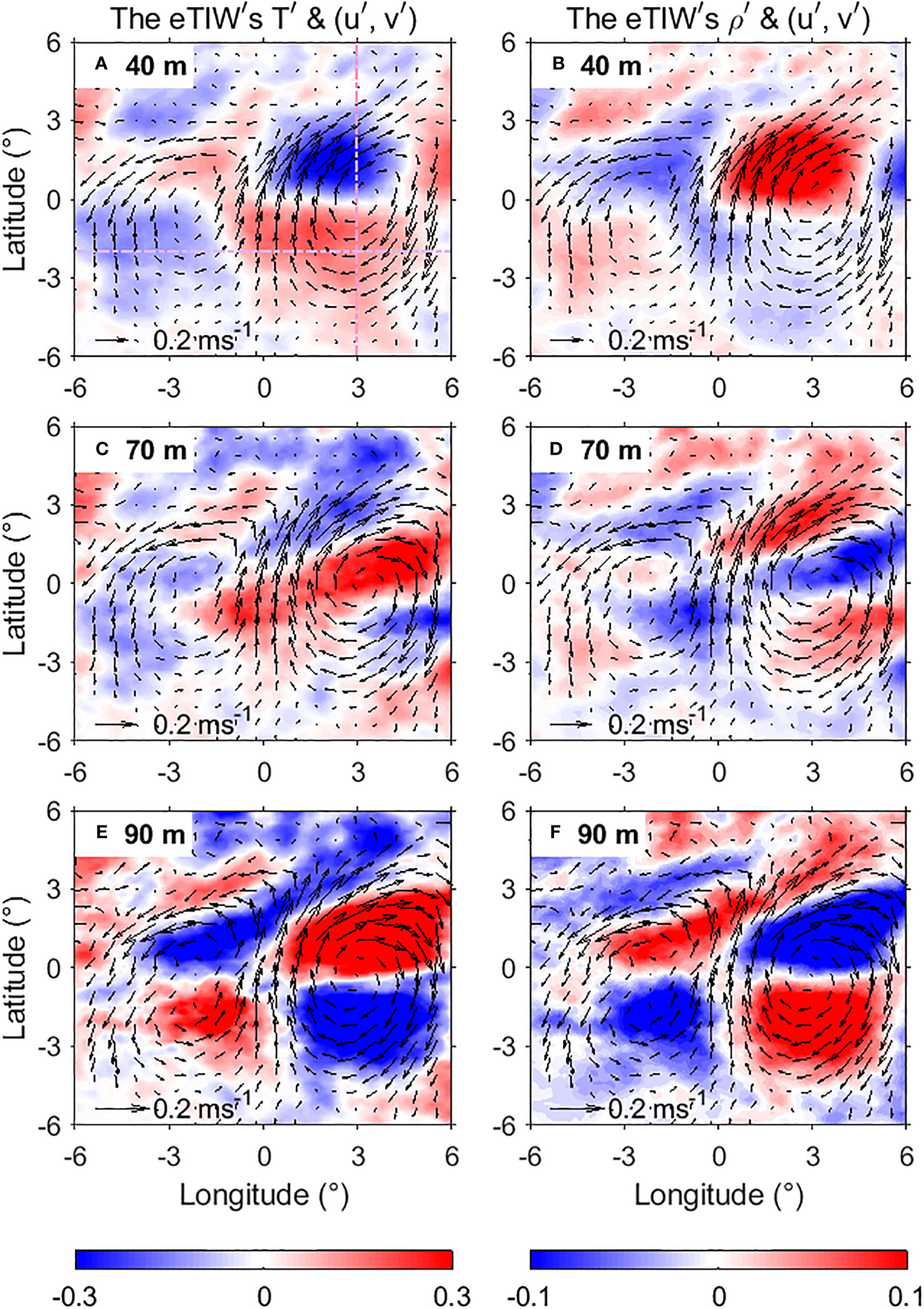
Figure 5 The composite of eTIW-associated temperature $T^{\prime }$ (shading, unit: °C), density ${\rho }^{\prime }$ (shading, units: kg·m⁻³) and velocities ($u^{\prime }, v^{\text{'}}$) (vectors, unit: ms⁻¹) at (A, B) 40 m, (C, D) 70 m, and (E, F) 90 m depths, respectively. The pink and purple dashed lines in (A) represent the zonal section (along 2°S) and meridional section (along 3°E) that will be used for representation of the eTIWs’ sectional structure in Figures 7, 10, 13, respectively.

2.2.1.4 Compositing the eTIW-associated SST with observations

For reference and comparison, we also obtain monthly (December) composite SST anomalies associated with eTIWs based on OISST data from 2008 to 2019 using a similar method as mentioned above (Figure 6). Note that, unlike the model results, the observational SST shows a periodic band of 12–28 days for the eTIWs. Therefore, the SST anomalies are obtained by applying a 12–28-day band-pass filter to the SST data. Subsequently, we record the time corresponding to the peak of SST anomalies at (136°W, 0°), which include 4 and 20 December 2008, 20 December 2009, 16 December 2010, 4 and 22 December 2011, 2 and 19 December 2012, 5 December 2013, 26 December 2014, 15 December 2015, 27 December 2016, and 11 and 27 December 2017, and finally composite the eTIW-associated SST anomalies.

FIGURE 6

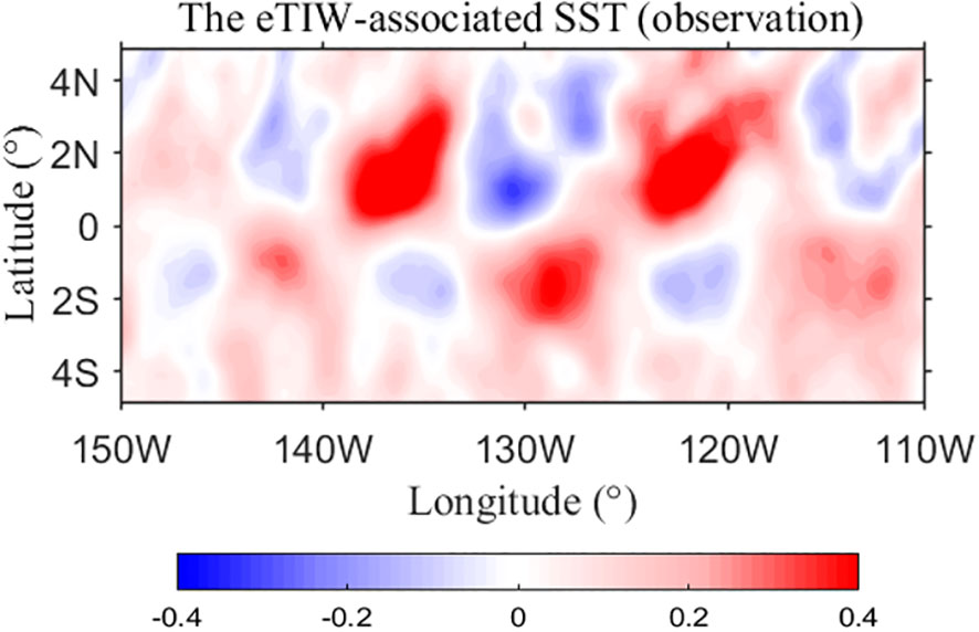
Figure 6 The composite eTIW-associated SST anomaly (°C) obtained from the OISST data in December 2008 to 2019.

2.2.2 Calculation of properties of shear instability and mixing

Stratification and velocity shear are the main factors in shear instability. Before the calculation of these factors, the original temperature and velocity data of the upper 300 m are interpolated into 2-m grid points. The density is derived from the temperature and salinity data from HYCOM. The stratification is represented by the squared buoyancy frequency, denoted as $N^2$. Here, $N^2=-\frac{\text{ɡ}}{{\rho }_0}\frac{\partial \rho }{\partial z}$, where ${\rho }_0=1,030\text{ kg} {\text{m}}^{-3}$, $\rho$ is the potential density, and $ɡ$ is the gravitational acceleration. The stratification distribution associated with eTIWs (denoted as $N^{2\prime }$) is obtained by applying a 12–24-day band-pass filter to the total $N^2$. The $N^2$ with a 45-day low-pass filtering is considered the background mean, denoted as $\overline{N^2}$. Meanwhile, the shear-squared anomalies resulted from eTIWs, $S^{\prime 2}$, are considered as the combination of the shear squared of themselves and their interaction with the mean flow, which is calculated using the following formula (Liu et al., 2019a; Liu et al., 2019b; Liu et al., 2020):

$\begin{array}{ll}S{\text{′}}^2=S_u^{\text{′}2}+S_v^{\text{′}2}=\left[{\left(\frac{\partial u\text{′}}{\partial z}\right)}^2+{\left(\frac{\partial v\text{′}}{\partial z}\right)}^2\right]+\left[2\frac{\partial \overline{U}}{\partial z}\frac{\partial u\text{′}}{\partial z}+2\frac{\partial \overline{V}}{\partial z}\frac{\partial v\text{′}}{\partial z}\right]& (1)\end{array}$

Here, the shear squared of the mean flow, ${\overline{S}}^2$ is calculated as $\overline{S^2}={(\frac{\partial \overline{U}}{\partial z})}^2+{(\frac{\partial \overline{V}}{\partial z})}^2$. In addition, the shear squared of the total flow, $S^2$, is calculated as $S^2={(\frac{\partial u}{\partial z})}^2+{(\frac{\partial v}{\partial z})}^2$. From case to case, the total shear can be largely modulated by the shear induced by the eTIWs. According to Eq. (1), the interaction between eTIWs and the mean flow (which is zonal) is described as when the sign of $\frac{\partial u\prime }{\partial z}$ is the same as that of $\frac{\partial \overline{U}}{\partial z}$, the total shear will be strengthened (Liu et al., 2019a; Liu et al., 2019b; Liu et al., 2020).

Finally, we use the RSS to characterize the mixing effect. It represents shear instability and encompasses velocity-associated shear and density-associated strain, which contribute to turbulence and mixing. The RSS associated with eTIWs at different depths can be derived from the stratification and shear squared anomalies, denoted as, $S_{\text{red}}^{\prime 2}=S^{\prime 2}-4N^{2\prime }$. Similarly, the RSS of the mean flow and the total flow are calculated as $\overline{S_{\text{red}}^2}=\overline{S^2}-4\overline{N^2}$ and $S_{\text{red}}^2=S^2-4N^2$, respectively.

3 The 3D structure of eTIWs

The characteristics of the eTIWs’ velocity field become apparent. Taking the depth of 40 m as an example (Figure 3A), the eTIW-associated velocity is concentrated at 5°S–3°N and shows typical characteristics of a Yanai wave, with the maximum zonal and meridional velocities reaching 0.17 and 0.31 m s⁻¹, respectively, at the equator. Additionally, similar to Liu et al. (2019a), the corresponding total flow presents an unclosed “S-shaped” structure due to the influence of the South Equatorial Current (SEC) (Figure 3B).

To shed light on their 3D structures, we now examine the vertical variation of their velocities above 300 m along a zonal section (along the equator, purple dotted line in Figure 3A) and a meridional (pink dotted line in Figure 3A) section (Figure 4). The results reveal that the eTIW-associated velocity is predominantly confined to the upper 120 m, above the thermocline. Near the equator (0°), $u^{\prime }$ seems to reverse around 120 m depth (Figure 4A). In the zonal section, the velocity near 0° (within 3°) exhibits a noticeable northeastward direction while oscillating southwestward on both sides (Figures 4A, C). In the specific meridional section (Figures 4B, D), the meridional velocity component remains generally weak. The eastward $u^{\prime }$ is strong at the north of the equator, while the westward $u^{\prime }$ is concentrated at the south of the equator (Figure 4B). At the same time, there is a northward $v^{\prime }$ at the north of the equator, while a southward $v^{\prime }$ at the south of the equator (Figure 4D). These structures confirm the NE-SW oscillation of the eTIWs, as initially identified by Liu et al. (2019a).

We then present the horizontal structure of the eTIW-associated temperature anomalies $T^{\prime }$, overlaid with the eTIW-associated velocity, at 40, 70, and 90 m depths (Figures 5A, C, E). At 40 m depth (Figure 5A), a centrosymmetric structure is observed at (0°, 0°). The negative values of $T^{\prime }$ are predominantly located in the northern part of the clockwise component and the southern part of the anticlockwise component, while positive values are distributed in the southern part of the clockwise component and the northern part of the anticlockwise component. This structure is consistent with that of Yanai waves. This pattern is also evident in satellite-based observational data in December, a month of obvious eTIWs (Figure 6). This pattern has also been observed and reported by Wang et al. (2020) with SST and sea surface height (SSH) data.

The depth of ~70 m is the vertical transition layer for $T^{\prime }$; above and below this layer, the sign of $T^{\prime }$ changes (Figure 5C). At ~90 m depth, the temperature shows a completely opposite pattern compared to 40 m, with a more pronounced and intense temperature anomaly (Figure 5E). The zonal (along 2°S, purple dotted line in Figure 5A) and meridional (along 3°E, pink dotted line in Figure 5A) sections further illustrate the vertical sign change of $T^{\prime }$ (Figures 7A, B). Specifically, above the transition depth of 70 m, the $T^{\prime }$ of the southern part of the clockwise component is positive; what is not shown by the figure is that the $T^{\prime }$ of the northern part of the anticlockwise component is also positive. In contrast, the northern part of the clockwise component and the southern part of the anticlockwise component are negative (Figures 7A, B). As depth increases (90–150 m), the sign of $T^{\prime }$ reverses (Figure 7A) from the upper layers. However, note that even though the temperature anomalies are large at these depths, they are accompanied by relatively weak velocity anomalies (Figure 5).

FIGURE 7

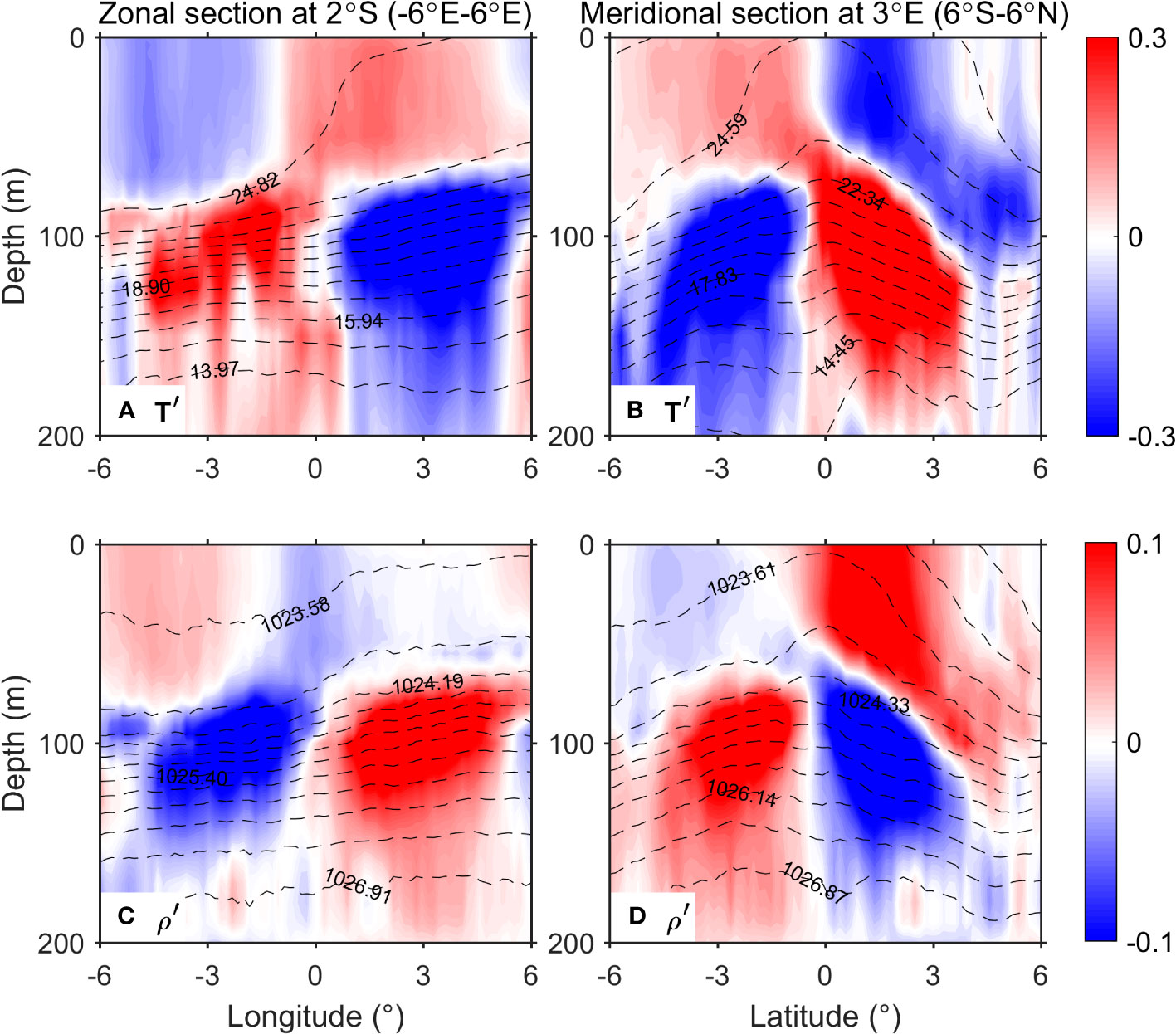
Figure 7 The composite of eTIW-associated temperature $T^{\prime }$ (shading, unit: °C) and density ${\rho }^{\prime }$ (shading, units: kg·m⁻³) along two sections above 200 m: (A, C) along the zonal section at 2°S and (B, D) along the meridional section at 3°E. The contours in (A) and (B) show the contours of the mean temperature and density, respectively. The locations of the sections are denoted in Figure 5A.

The horizontal structure of the density anomalies ${\rho }^{\prime }$ at the three depths is also shown in Figures 5B, D, F. It can be observed that ${\rho }^{\prime }$ is mainly determined by $T^{\prime }$.

To our knowledge, this is the first time that the detailed spatial structure of the temperature of the eTIW is presented. However, a structure represented by complex empirical orthogonal functions (CEOFs) analysis (amplitude and phase of CEOF) was previously provided by Lyman et al. (2007; their Figure 14). Their analysis revealed meridional antisymmetry about the equator and vertical phase reversal in temperature—the phase of temperature showed a 90° reversal between ~60 m and ~80 m, and a 180° reversal between ~80 m and ~140 m. As argued by Lyman et al. (2007), the vertical changes in signs of $T^{\prime }$ and ${\rho }^{\prime }$ represent the first baroclinic mode, obviously. Therefore, our results confirm and complement Lyman’s by showing 3D temperature variations. Consequently, as will be shown in the following section, these specific density and shear structures, both horizontally and vertically, are of great importance for the eTIW-associated shear instability and mixing properties.

We also constructed the eTIW-associated salinity structure (Figure 8). Relative to the temperature, few studies have been done on the TIW-induced salinity structure (Lee et al., 2012; Yin et al., 2014; Lee et al., 2015), and to our knowledge, no research has even been focused on the eTIW-associated salinity yet. In the upper thermocline layers (40–70 m), the salinity pattern appears relatively regular, exhibiting antisymmetric about the meridional center and showing a dipole structure. This is quite different from the temperature structure. The maximum and minimum salinities are mainly concentrated at 5°S–3°N along the equator. Vertically, there is no obvious phase reversal at different depths. Positive salinity anomalies appear to occur in the clockwise flow field and negative anomalies in the anticlockwise flow field. This seems to be related to the downwelling and upwelling effects due to the eTIW-associated flows. Below 70 m, the salinity distribution tends to be irregular with an increase in depth. Despite the significant spatial pattern, the salinity changes do not contribute much to the density changes (Figures 5, 7), and therefore, they are not further analyzed in the present study.

FIGURE 8

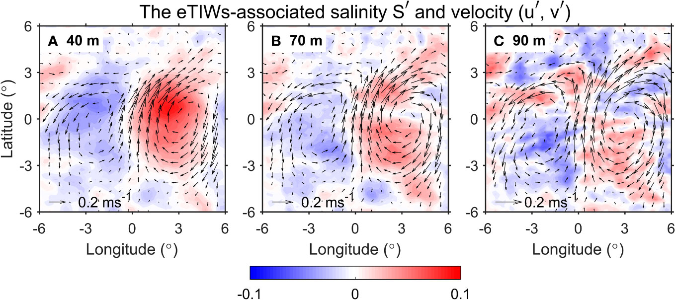
Figure 8 The composite of eTIW-associated salinity $S^{\prime }$ (shading, unit: PSU) and velocities ($u^{\prime },v^{\prime }$) (vectors, unit: ms⁻¹) at (A) 40 m, (B) 70 m, and (C) 90 m depths, respectively.

FIGURE 9

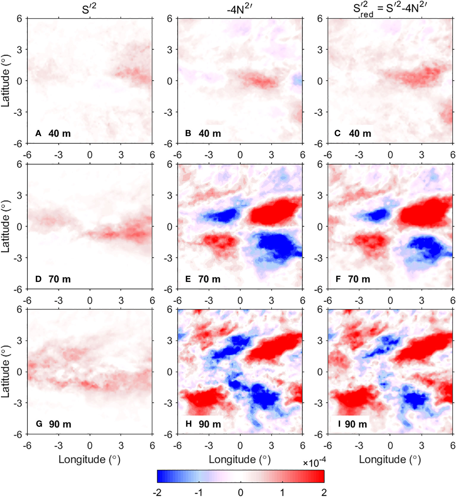
Figure 9 The composite of eTIW-associated shear squared $S^{\prime 2}$, buoyancy frequency squared multiplied by a factor of −4, $-4N^{2\text{'}}$, and reduced shear squared $S_{\text{red}}^{\prime 2}=S^{\prime 2}-4N^{2\text{'}}$, respectively, at (A–C) 40 m, (D–F) 70 m, and (G–I) 90 m (unit: s⁻²).

4 Shear instability and mixing properties

The mixing process and its effects in the central and eastern equatorial Pacific have been of widespread interest. In this section, we shed light on the structural characteristics of associated stratification, shear squared, and RSS, building upon the distribution characteristics of each fundamental property associated with eTIWs. The goal is to elucidate the impacts of eTIWs on equatorial shear stability and mixing.

4.1 The stratification and RSS associated with the eTIWs

The stratification ($N^{2\prime }$, times −4), shear squared ($S^{\prime 2}$), and RSS ($S_{\text{red}}^{\prime 2}$) structure associated with the eTIWs at different depths of 40, 70, and 90 m are given in Figure 10.

FIGURE 10

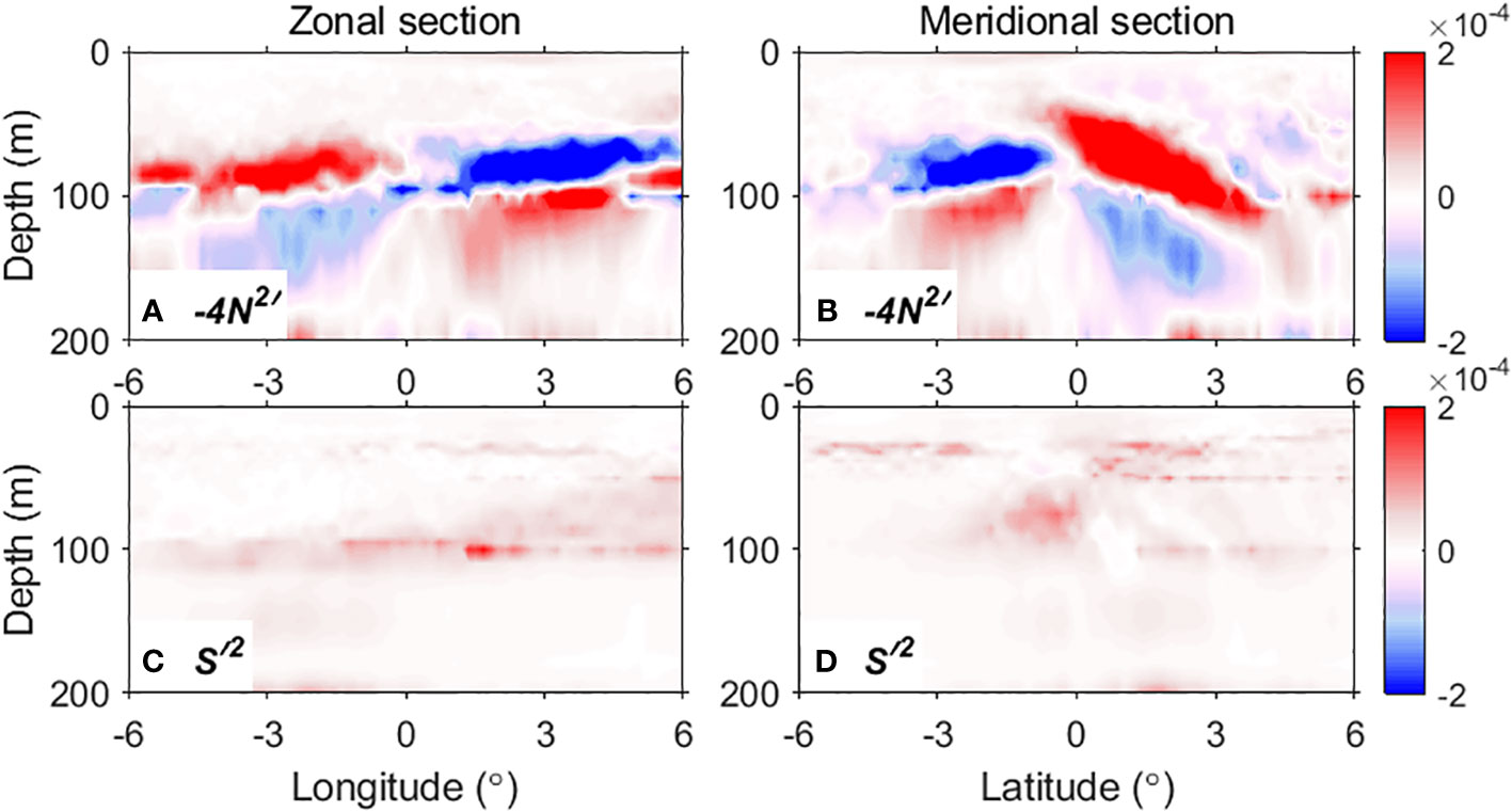
Figure 10 The composite of eTIW-associated buoyancy frequency squared multiplied by a factor of −4, $-4N^{2\prime }$, and shear squared $S^{\prime 2}$, respectively, along (A, C) zonal and (B, D) meridional sections (unit: s⁻²). The location of the sections are denoted in Figure 5A.

FIGURE 11

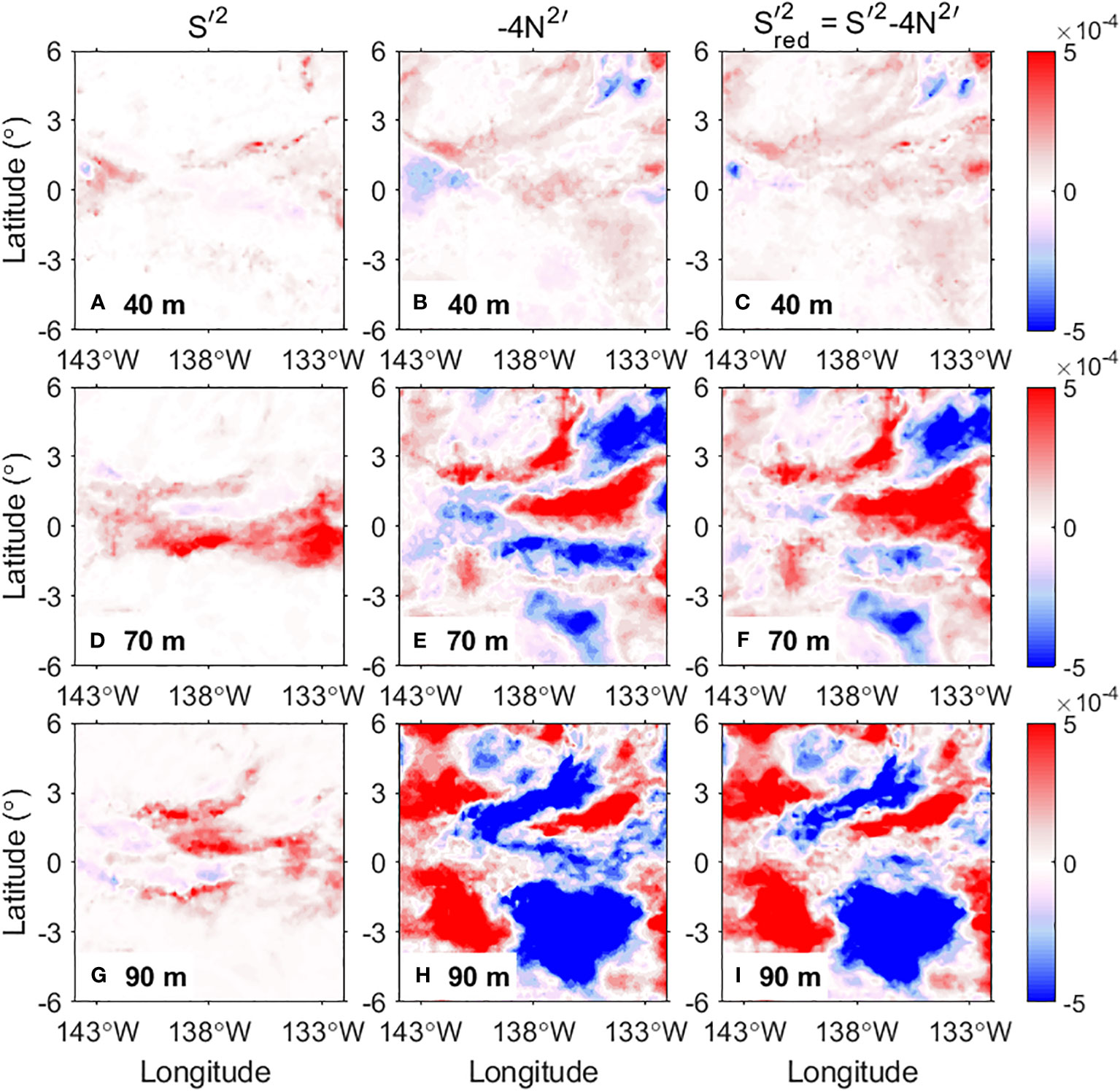
Figure 11 The same as Figure 9, but for daily variables on 20 December 2000.

It is found that in the upper layer of 40 m (Figures 9B, C), both the eTIW-induced stratification and RSS anomalies are weaker, except for a weakly positive region at (0°–4°E, 0°–1.5°N). As the depth reaches 70 m, the stratification and RSS anomalies become strong, and a centrosymmetric structure appears in the composite region (Figures 9E, F). The intensity distribution of stratification of eTIWs is evident near 70 m, which aligns with the vertical shifts in temperature and density (Figures 5, 9E). In this region, the density is mainly determined by temperature (Smyth and Moum, 2013), which is confirmed by Figures 5, 7. At around 70 m, the eTIW-associated $T^{\prime }$ and ${\rho }^{\prime }$ are obvious, and their vertical changes are large, leading to obvious $N^{2\prime }$ structures (Figure 7). Positive $-4N^{2\prime }$ are located at the northern part (0°–6°E, 0–3°N) of the clockwise flow field and the southern part (−3°–0°E, 0°–3°S) of the anticlockwise component. In the meantime, the negative $-4N^{2\prime }$ are mainly located at the southern part (0°–6°E, 0°–4°S) of the clockwise flow field and the northern part (–3°–0°E, 0°–2°N) of the anticlockwise flow field. The reduced stratification of eTIWs (positive $-4N^{2\prime }$) may be favorable for shear instability. In the other two regions, stratification is strong which tends to stabilize the flow.

While the pattern of $-4N^{2\prime }$ at 90-m depth almost resembles that at 70 m (Figure 9H), the differences show up. An obvious difference is that the pattern with a large magnitude of $-4N^{2\prime }$ expands poleward, leaving a relatively wide equatorial band of low stratification variation. However, the most significant difference is that the signs of $-4N^{2\prime }$ reverse below the transition layer at ~100 m (Figures 10A, B), which reflects the vertical variations of temperature and density, as shown in Figure 7.

For the structure of $S^{\prime 2}$, at 40 m, there is a weak shear structure at (2°–6°E, 1°S–3°N) covered by the clockwise flow (Figure 9A). As the depth increases (Figures 9D, G), at 70 m, the shear becomes stronger in the northern part of the anticlockwise flow at (–6°–0°E, 1°S–2°N), and in the southern part of the clockwise flow at (0°–6°E, 3°S–2°N). This pattern is in contrast to that of $-4N^{2\prime }$. However, the strong shear is confined only in the equatorial band at lower layers, which results from the strong vertical shear of the Equatorial Undercurrent (EUC) and the interaction with the shear of the eTIW (Liu et al., 2019a; Liu et al., 2019b; Liu et al., 2020). At 90 m, the strong shear region expands to 3°S–3°N. Note that, at all depths, eTIWs induce all positive $S^{\prime 2}$. Viewed from the perspective of the vertical section (Figures 12C, D), $S^{\prime 2}$ is found particularly enhanced in some specific regions: the southern part of the clockwise component between 3°S–0°N, 0°–6°E, and 50 ~110 m, and the northern part of the clockwise component between 20 m and 50 m. Those regions are where the eTIW-induced vertical shear (Figure 4) has the same sign as that of the mean flow, thus $S^{\prime 2}$ is enhanced according to Eq. (1).

FIGURE 12

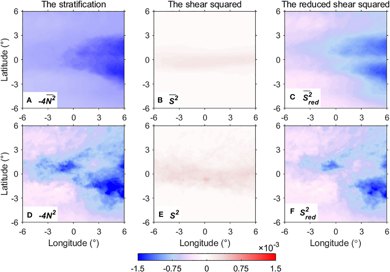
Figure 12 The composite of stratification, velocity shear squared, and reduced shear squared of (A–C) the mean flow and (D–F) the total flow at 70 m depth respectively (unit: s⁻²).

By comparing the $N^{2\prime }$, $S{"}^2$, and $S_{\text{red}}^{\prime 2}$ at different depths, it is found that the $N^{2\prime }$, rather than $S{\prime }^2$, plays the dominant role in determining the $S_{\text{red}}^{\prime 2}$ pattern in the thermocline. Figure 9F shows obviously the centrosymmetric structure of the $S_{\text{red}}^{\prime 2}$ at the depth of 70 m, which is basically consistent with the $-4N^{2\prime }$ in structure. The positive $-4N^{2\prime }$ correspond to the positive $S_{red}^{\prime 2}$, and vice versa. The magnitudes of $-4N^{2\prime }$ and $S_{\text{red}}^{\prime 2}$ are also similar, while $S^{\prime 2}$ is usually several factors to 1–2 orders smaller than them (Figures 9D–F, 10A–D). However, at some locations where $S{\prime }^2$ is strong, its contribution to $S_{\text{red}}^{\prime 2}$ is also noticeable.

This conclusion is also confirmed by snapshots of eTIW-associated $-4N^{2\prime }$, $S{\prime }^2$, and $S_{\text{red}}^{\prime 2}$. We investigated the 27 daily samples and selected a sample that has the most unstable conditions (Ri< 0.25) at 70 m among all the samples to plot the pattern of the above variables (Figure 11). It is found that, besides many intermittent structures that manifested as submesoscale patches, the eTIW-associated mesoscale pattern is dominant. Particularly, in any of the submesoscale or mesoscale patterns, it is shown that $-4N^{2\prime }$ makes a larger contribution than $S{\prime }^2$ to $S_{\text{red}}^{\prime 2}$. An exception is that, close to the equator (Figure 11D), $S{\prime }^2$ could contribute more than $-4N^{2\prime }$, where the former is large while the latter is very weak.

Unlike the previous studies, which emphasize the effect of TIW’s velocity shear on mixing, the finding highlights that the stratification of eTIWs is the major modulating factor in its RSS pattern (thus turbulence or mixing). This discovery has important implications for understanding mixing processes in the equatorial Pacific. This result confirms Liu et al. (2020), who revealed that equatorial waves of varying scales have different strain anomalies (i.e., $N^{2\prime }$), which can be comparable to or even larger than the shear anomalies. It should be noted that similar to shear anomalies, the stratification plays the role of generating mixing only during specific phases of the waves.

4.2 Mixing effect of eTIWs on the total flow

The occurrence of TIWs is primarily observed in the central to eastern equatorial Pacific, where the mean flow consists of a westward-flowing SEC on the surface layers and an eastward EUC in the subsurface layers. This configuration generates an up-westward background vertical shear. Due to the combined modulation by different dynamical kinds of equatorial waves and small-scale shear instability, mixing events are frequent in this region (Liu et al., 2020). In this study, we investigate the specific effects of the eTIWs on shear instability and mixing in the context of the mean flow. To simplify the analysis, we follow the approach of Liu et al. (2020) and use the 45-day low-pass filtered velocity as a representation of the “mean flow.” The occurrence of shear instability depends on the sign of the total RSS, which is approximately the sum of both the mean flow and the eTIW-associated anomalies. If the total RSS is positive (negative), shear instability will occur (will not occur). Therefore, the total RSS serves as an indicator of the occurrence of shear instability.

Firstly, we focus on the depth of 70 m, which serves as a representative layer of the thermocline, to investigate the properties related to instability and mixing associated with eTIWs. As shown already, the mean stratification is mainly affected by the temperature of the mean flow, and the results reflect the temperature characteristics of the equatorial cold tongue region (Figure 12A). Within the range of 3°S–3°N, $-4\overline{N^2}$ is relatively small (the magnitude is large) with a minimum value of −1.40 × 10⁻³ s⁻², indicating a strong inhibiting effect on shear instability; meanwhile, $-4\overline{N^2}$ gradually decreases from west to east, representing the fact that the stratification is stronger in the east than west in the study region. Off the 3°S–3°N band, $-4\overline{N^2}$ becomes larger (the magnitudes become smaller; Figure 12A).

FIGURE 13

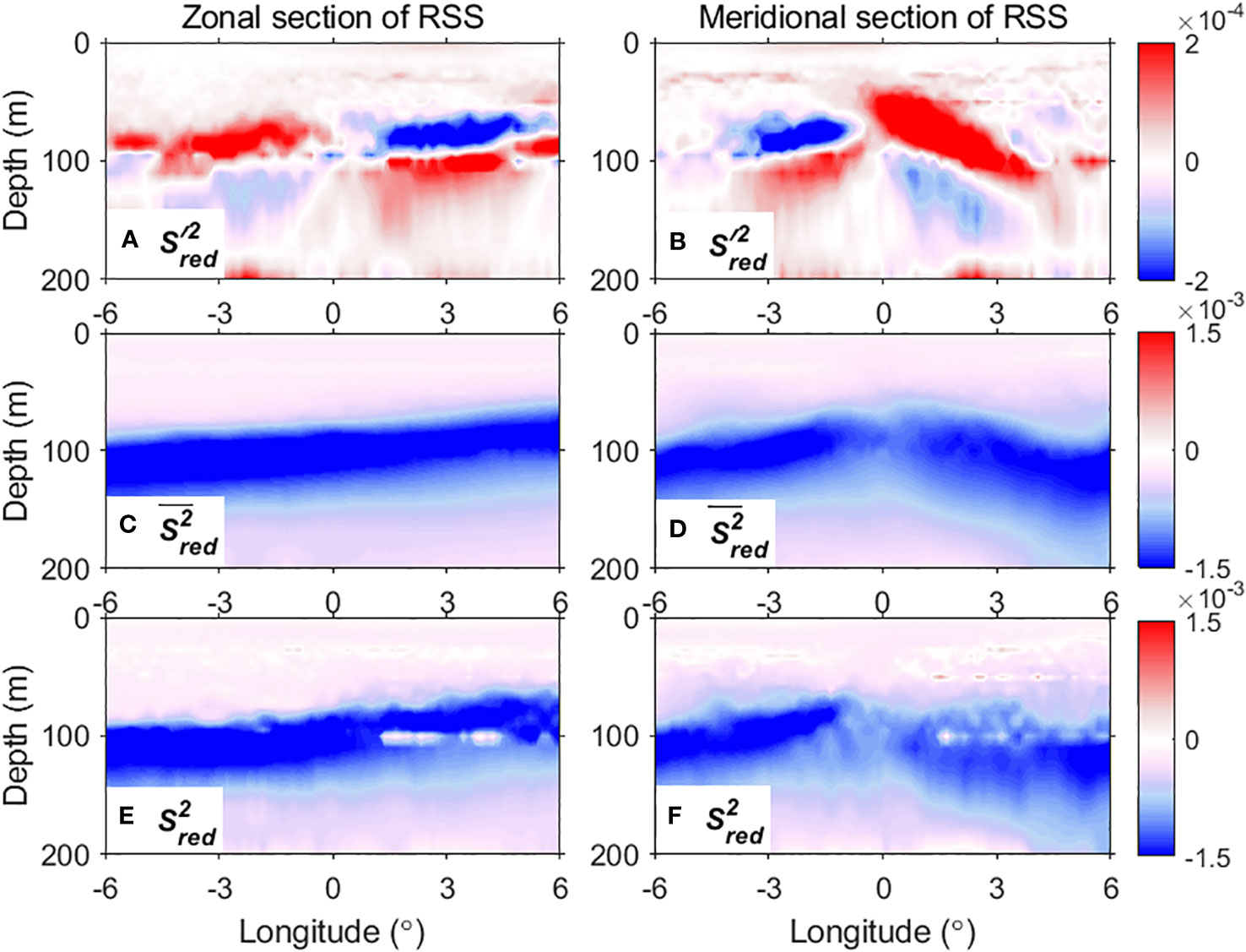
Figure 13 Composite of the reduced shear squared (RSS) of (A, B) the eTIWs, (C, D) the mean flow, and (E, F) the total flow (unit: s⁻²).

At this depth, the shear squared of the mean flow $\overline{S^2}$ is featured as an equatorial band (1°S–1°N) maximum of 2.46 × 10⁻⁴ s⁻² (Figure 12B). Off this band, the shear squared is considerably weak. In total, the RSS pattern of the mean flow $\overline{S_{\text{red}}^2}$ at this depth is determined by both the $-4\overline{N^2}$ and $\overline{S^2}$, and is negative in general (corresponding to a stable state). However, in the west and along the equator (Figure 12C), due to the contribution of the mean shear squared $\overline{S^2}$, the $\overline{S_{\text{red}}^2}$ is closer to 0, i.e., the state tends to be subject to marginal instability.

The stratification of eTIWs has comparable magnitudes to the stratification of the mean flow, which therefore modulates the total stratification largely, particularly near the equator (Figure 9E). The negative stratification anomalies of eTIWs (positive $-4N^{2\prime }$) weakens the stratification of the total flow field at the northern part of the clockwise component and the southern part of the anticlockwise component (Figure 12D). On the contrary, the positive stratification of eTIWs (negative $-4N^{2\prime }$) strengthens the stratification of the total flow field at the southern part of the clockwise component and the northern part of the anticlockwise component.

In comparison to $\overline{S^2}$, the shear squared of the eTIWs $S^{\prime 2}$ is weaker, but also becomes comparable in specific regions close to the equator, including the northern part of the anticlockwise flow at (–6°–0°E, 1°S–2°N) and in the southern part of the clockwise flow at (0°–6°E, 2°S–1°N) (Figure 9D), which modulate the total shear squared $S^2$ obviously (Figure 12E).

Overall, it is seen that, at specific phases, the eTIW-associated shear squared $S^{\prime 2}$ and stratification $-4N^{2\prime }$ can be comparable to that of the stratification $-4\overline{N^2}$ and shear squared $\overline{S^2}$ of the mean flow, respectively, so that the eTIWs efficiently modulate the total stratification $N^2,$ the shear squared $S^2$, and the total reduced shear squared $S_{\text{red}}^2$ (Figures 12D–F). For example, at 4°E, 2°N, due to the influence of positive $S_{\text{red}}^{\prime 2}$, the $S_{\text{red}}^2$ increases from –1.06 × 10⁻³ s⁻² to −7.42 × 10⁻⁴ s⁻², which is closer to the critical value 0 and favors the occurrence of instability (hence mixing).

In the vertical sections, three regimes can be classified for the stability of the mean flow (Figures 13C, D). Firstly, a regime of marginal instability is from the surface to the upper thermocline, where the $\overline{S_{\text{red}}^2}$ values are mainly between −4 × 10⁻⁴ s⁻² and −0.5 × 10⁻⁴ s⁻², close to zero; this regime is thicker in the west and off-equatorial band (~90 m) but shallower in the east and along the equator (~50 m). Previous studies based on data of 140°W, 0°N have demonstrated that this layer is subject to marginal instability (Smyth and Moum, 2013; Zhang et al., 2023). Secondly, the equatorial thermocline with a thickness of about 50–100 m at ~50–150 m is a regime of stability, where the $\overline{S_{\text{red}}^2}$ values range from −2 × 10⁻³ s⁻² to −1 × 10⁻³ s⁻². Thirdly, below the thermocline, it again becomes a regime of nearly marginal instability.

The eTIWs lead to an obvious vertical variation of $S_{\text{red}}^{\prime 2}$ (Figures 13A, B), with the pattern being primarily determined by the eTIW-associated stratification changes $-4N^{2\prime }$ and modulated by shear squared changes $S{\prime }^2$ in specific regions (Figures 10A, B). The $S_{\text{red}}^{\prime 2}$ is weak at upper 60 m but shows strong variations from 60 m to 90 m (Figures 13A, B). Either zonally or meridionally, the $S_{\text{red}}^{\prime 2}$ shows positive and negative phases; below ~100 m (100–150 m), the phase of $S_{\text{red}}^{\prime 2}$ is opposite to that of the upper layer between 60 m and 90 m, and the magnitude is very significant (Figures 13A, B). Consequently, the RSS of the total flow, $S_{\text{red}}^2$, though primarily determined by $\overline{S_{\text{red}}^2}$ (or $-4\overline{N^2}$), is greatly modulated by $S_{\text{red}}^{\prime 2}$ (Figures 13E, F), particularly in the regime of marginal instability in the upper layers. For example, at 1.5°N in the meridional section, the $\overline{S_{\text{red}}^2}$ at ~50 m is −4.44 × 10⁻⁴ s⁻², but under the influence of positive $S_{\text{red}}^{\prime 2}$, $S_{\text{red}}^2$ becomes 7.77 × 10⁻⁴ s⁻², being positive, which will lead to shear instability and mixing. Similar areas include the 20–40-m depth range along both zonal and meridional sections, the 40–60-m depth range from 1° to 4.5°N in the meridional section, and the 90–110 m depth range from 1° to 4.5°E in the zonal section.

5 Summary and discussion

This study focuses on the eTIWs in the Pacific Ocean and investigates their 3D structures and mixing effects on the equatorial flows. Horizontally, the eTIW-associated temperature and density show a centrosymmetric structure above 200 m. Above 70 m, positive (negative) temperature anomalies are observed in the southern (northern) part of the clockwise flow and the northern (southern) part of the anticlockwise flow field, which further determines the density pattern. Near ~70 m depth, the vertical phase transition occurs. Below this depth, temperature and density anomalies change into the opposite phase compared to that of the upper layer, indicating that the derived eTIW could be the first baroclinic mode of the Yanai wave-initiated instability wave.

The mixing effect of the eTIWs is revealed by analyzing the eTIW-associated RSS, which is composed of both the eTIW-associated shear squared and stratification components. In general, significant eTIW-associated shear squared is confined close to the equator, along with the westward velocity component in both phases of the eTIW; while patches of the shear squared can be comparable in magnitude to that of the eTIW-associated stratification, it is usually smaller than the latter. The eTIW-associated stratification anomaly reflects that of a Yanai wave-induced density anomaly, as described in the above paragraph. As a result, the eTIW-associated RSS shows a centrally symmetric structure at the upper layers in the leading order, which is illustrated by the schematic Figure 14. However, it is modulated by the specific background density structures in the central equatorial Pacific and by eTIW-associated shear squared. The positive values of the RSS in the upper layers (~40–90 m) are mainly distributed in the northern part of the clockwise component and the southern part of the anticlockwise component, respectively, which has the potential to lead to shear instability and mixing, particularly in the regime of original marginal instability. Note that, since both the eTIW-associated shear squared and stratification are weak in the mixed layer, the eTIW’s effect on the mixed layer mixing might be insignificant.

FIGURE 14

Figure 14 Schematics of the reduced shear squared (RSS) of the eTIW at (A) 40 m, 90 m, and 140 m depths and (B) on the 3°E and −3°E sections (units: s⁻²). Shown is based on 3D-smoothed composite RSS data, as shown in Figures 13A, B.

This finding is different from and complementary to previous understandings. Firstly, it was widely recognized that the vertical shear of eTIW ($S{\prime }^2$) and its interaction with the mean shear are the prevailing factors for the generation of shear instability and mixing. On the contrary, the present study reveals the dominant effect of the stratification of eTIWs ($-4N^{2\prime }$) in leading to shear instability conditions. Besides velocities, density and hence stratification also change associated with eTIW, which reflect the dynamical characteristics of Yanai waves. Possibly, the eTIW-associated velocities are not strong enough to dominate the RSS. However, whether this result applies to the Rossby wave-initiated TIWs needs further investigation because a Rossby wave-initiated TIW can induce strong (~1 m/s) velocity changes. Secondly, due to a lack of observations, previous studies usually focused on a single observation site (e.g., 140°W, 0°N); in contrast, this study provides the 3D structure, which extends poleward to ±5°, showing a wider view of the eTIW’s effect on mixing. The accumulated effect of the wide range of mixing should be important to heat redistribution in the equatorial band but has not been revealed yet. Lastly, we are aware that the eTIW’s mixing effect presented in this study is only indicated by its associated RSS anomalies derived from a numerical model rather than by observed metrics like turbulent kinetic energy dissipation rate or diffusivity; turbulence measurements might be conducted in the future to reveal more features and implications.

Data availability statement

The datasets presented in this study can be found in online repositories. The names of the repository/repositories and accession number(s) can be found in the Acknowledgments.

Author contributions

LF performed the data analysis and wrote the draft. CL initiated the idea of the study and rewrite the manuscript. FW supervised the findings of this work. All authors discussed the results and contributed to the final manuscript. All authors contributed to the article and approved the submitted version.

Funding

This study is supported by the National Natural Science Foundation of China (NSFC) (41976012, E12117106B), the Key Research Program of Laoshan Laboratory (LSKJ202202502), and the Strategic Priority Research Program of the Chinese Academy of Sciences (XDB42000000).

Acknowledgments

The dataset sources are greatly appreciated: the HYCOM data at the Asia-Pacific Data-Research Center (APDRC, http://apdrc.soest.hawaii.edu/) and the OISST data at National Oceanic and Atmospheric Administration (NOAA, https://www.ncei.noaa.gov/products/optimum-interpolation-sst/).

Conflict of interest

The authors declare that the research was conducted in the absence of any commercial or financial relationships that could be construed as a potential conflict of interest.

Publisher’s note

All claims expressed in this article are solely those of the authors and do not necessarily represent those of their affiliated organizations, or those of the publisher, the editors and the reviewers. Any product that may be evaluated in this article, or claim that may be made by its manufacturer, is not guaranteed or endorsed by the publisher.

References

Cherian D., Whitt D. B., Holmes R. M., Lien R. C., Bachman S., Large W. G. (2020). Off-equatorial deep cycle turbulence forced by Tropical Instability Waves in the equatorial Pacific. J. Phys. Oceanogr. 51, 1575–1593. doi: 10.1175/JPO-D-20-0229.1

CrossRef Full Text | Google Scholar

Flament P. J., Kennan S. C., Knox R. A., Niiler P. P., Bernstein R. L. (1996). The three-dimensional structure of an upper ocean vortex in the tropical Pacific Ocean. Nature 383, 610–613. doi: 10.1038/383610a0

CrossRef Full Text | Google Scholar

Holmes R. M., Thomas L. N. (2015). The modulation of equatorial turbulence by tropical instability waves in a regional ocean model. J. Phys. Oceanogr. 45, 1155–1173. doi: 10.1175/JPO-D-14-0209.1

CrossRef Full Text | Google Scholar

Inoue R., Lien R. C., Moum J. N. (2012). Modulation of equatorial turbulence by a tropical instability wave. Geophys. Res. Lett. 117, C10009. doi: 10.1029/2011JC007767

CrossRef Full Text | Google Scholar

Lee T., Lagerloef G., Gierach M. M., Kao H. Y., Yueh S., Dohan K. (2012). Aquarius reveals salinity structure of tropical instability waves. Geophys Res. Lett. 39, L12610. doi: 10.1029/2012GL052232

CrossRef Full Text | Google Scholar

Lee T., Lagerloef G., Kao H. Y., Mcphaden M. J., Willis J., Gierach M. M. (2015). The influence of salinity on tropical Atlantic instability waves. J. Geophys Res. 119, 8375–8394. doi: 10.1002/2014JC010100

CrossRef Full Text | Google Scholar

Liu C., Fang L., Köhl A., Liu Z., Smyth W. D., Wang F. (2019b). The subsurface mode tropical instability waves in the equatorial Pacific ocean and their impacts on shear and mixing. Geophys. Res. Lett. 46, 12270–12278. doi: 10.1029/2019GL085123

CrossRef Full Text | Google Scholar

Liu C., Köhl A., Liu Z., Wang F., Stammer D. (2016). Deep-reaching thermocline mixing in the equatorial pacific cold tongue. Nat. Commun. 7, 11576. doi: 10.1038/ncomms11576

PubMed Abstract | CrossRef Full Text | Google Scholar

Liu C., Wang X., Köhl A., Wang F., Liu Z. (2019a). The northeast-southwest oscillating equatorial mode of the tropical instability wave and its impact on equatorial mixing. Geophys. Res. Lett. 46, 218–225. doi: 10.1029/2018gl080226

CrossRef Full Text | Google Scholar

Liu C., Wang X., Liu Z., Köhl A., Smyth W. D., Wang F. (2020). On the formation of a subsurface weakly sheared laminar layer and an upper thermocline strongly sheared turbulent layer in the eastern equatorial Pacific: Interplays of multiple-time-scale equatorial waves. J. Phys. Oceanogr. 50, 2907–2930. doi: 10.1175/JPO-D-19-0245.1

CrossRef Full Text | Google Scholar

Lyman J. M., Johnson G. C., Kessler W. S. (2007). Distinct 17- and 33-day tropical instability waves in subsurface observations*. J. Phys. Oceanogr. 37, 855–872. doi: 10.1175/jpo3023.1

CrossRef Full Text | Google Scholar

Moum J. N., Lien R. C., Perlin A., Nash J. D., Gregg M. C., Wiles P. J. (2009). Sea surface cooling at the equator by subsurface mixing in tropical instability waves. Nat. Geosci. 2, 761–765. doi: 10.1038/ngeo657

CrossRef Full Text | Google Scholar

Smyth W. D., Moum J. N. (2013). Marginal instability and deep cycle turbulence in the eastern equatorial Pacific Ocean. Geophys. Res. Lett. 40 (23), 6181–6185. doi: 10.1002/2013GL058403

CrossRef Full Text | Google Scholar

Wang M., Xie S., Shen S. S. P., Du Y. (2020). Rossby and Yanai modes of tropical instability waves in the equatorial Pacific ocean and a diagnostic model for surface currents. J. Phys. Oceanogr. 50, 3009–3024. doi: 10.1175/JPO-D-20-0063.1

CrossRef Full Text | Google Scholar

Warner S. J., Holmes R. M., Hawkins E. H., Hoecker-Martínez M. S., Savage A. C., Moum J. N. (2018). Buoyant gravity currents released from tropical instability waves. J. Phys. Oceanogr. 48, 361–382. doi: 10.1175/JPO-D-17-0144.1

CrossRef Full Text | Google Scholar

Whitt D. B., Cherian D., Holmes R. M., Bachman S., Lien R. C., Large W. G., et al. (2021). Simulation and scaling of the vertical heat transport in deep-cycle turbulence throughout the equatorial Pacific cold tongue. J. Phys. Oceanogr. 52, 981–1014. doi: 10.1175/JPO-D-21-0153.1

CrossRef Full Text | Google Scholar

Yin X., Boutin J., Reverdin G., Tong L., Arnault S., Martin N. (2014). SMOS sea surface salinity signals of tropical instability waves. J. Geophys. Res. 119, 7811–7826. doi: 10.1002/2014JC009960

CrossRef Full Text | Google Scholar

Zhang J., Liu C., Gong X., Wang F. (2023). Persistent mixing bursts in the equatorial pacific thermocline induced by persistent equatorial waves. J. Oceanology Limnology. doi: 10.1007/s00343-023-2350-z

CrossRef Full Text | Google Scholar