 Sajjad Feizabadi
 Chunyan Li
 Matthew Hiatt
95% of researchers rate our articles as excellent or good
Learn more about the work of our research integrity team to safeguard the quality of each article we publish.
Find out more
ORIGINAL RESEARCH article
Front. Mar. Sci. , 29 September 2023
Sec. Physical Oceanography
Volume 10 - 2023 | https://doi.org/10.3389/fmars.2023.1228446
The effects of passing atmospheric cold fronts with different orientations and moving directions on the hydrodynamics of the Wax Lake Delta (WLD) were analyzed by considering the influence of river discharge, cold front moving direction, wind magnitude, and Coriolis effect. The study employs numerical simulations using the Delft-3D model and an analytical model to explore water volume transport, water level variations, water circulation, and particle trajectories during nine cold front events. Results indicate that cold fronts cause a decrease in the average contribution of the water transport through western channels and an increase of that in central and eastern channels. A westerly cold front with an average wind speed of ~12 m/s can increase water transport through eastern channels by about 35%. During the passage of a cold front, the intertidal islands between the main channels and East Bay experience the largest fluctuations in subtidal water levels, which can be attributed to the influence of local wind stress. For example, a westerly cold front can result in a water level variation of approximately 0.45 m over some of the intertidal Islands and 0.65 m in the East Bay. Results also show that the subtidal water circulation in the WLD is correlated with the Wax Lake Outlet (WLO) discharge and wind magnitude. The findings illustrate that when WLO discharge is low, the impact of cold fronts is more pronounced, and cold fronts from the west have a greater impact compared to those from the northwest and north. This study identifies the significance of WLO discharge and Coriolis force by the trajectories of particles in the water column. The results of the simulations indicate that under low WLO discharge (less than 2000 m3/s), the majority of particles are found to exit through Campground Pass instead of Gadwall because of the dominance of Coriolis force. To summarize, this study assesses the impact of cold fronts on the hydrodynamics of the Wax Lake Delta, underscoring the contributions of multiple factors, including the cold front moving direction, river discharge, wind strength, and Coriolis force.
A cold front is the leading edge of a cooler mass of air moving against a warmer mass of air (Hsu, 1988). Cold fronts are recurring phenomena with a time interval of approximately 3–7 days (Roberts et al., 1989). A 40-year statistical review of weather data revealed that coastal Louisiana experiences 41 ± 5 cold front passages every year between October and the following April (Li et al., 2020). Before a typical frontal passage (pre-frontal) in coastal Louisiana, southerly and easterly winds drive shelf water to the shore. This causes an influx of water into coastal bays, which can increase water level by 0.3 to 0.5 m (Denes and Caffrey, 1988; Childers and Day, 1990). After the cold front passes (post-frontal), winds often change to northerlies in a rotary fashion, e.g., westerly and then northerly and northeasterly, and water quickly drains from the shallow marshes and bays (Hsu, 1988). Previous studies illustrated that the regular flooding and draining induced by cold front passages are the primary transport mechanisms for water, sediment, nutrients, and organic matter through coastal bays in the northern Gulf of Mexico during winter months (Childers and Day, 1990; Li et al., 2011; Li, 2013; Huang and Li, 2017; Chaichitehrani et al., 2019).
Over the past few years, there have been many studies conducted on hydrodynamics in response to atmospheric forces and water transport in the estuaries of the Atlantic and Gulf coasts (e.g., Snedden et al., 2007; Salas-Monreal and Valle-Levinson, 2008; Hiatt et al., 2019; Feizabadi et al., 2022; Zhang et al., 2022). However, the Louisiana estuaries have their own characteristics, mostly due to the geomorphology features, low-tidal amplitude, and meteorological conditions between the subtropics and mid-latitude. Estuaries in coastal Louisiana are often bar-built, longitudinally short, and shallow (typically less than 3 m). Tides in the region are dominated by diurnal constituents with a maximum tidal range of approximately 0.6 m (Kantha, 2005), contrasting with tides in the east coast, which are predominantly semi-diurnal (Pritchard, 1952) with higher amplitudes. Therefore, the effects of atmospheric forces are relatively more important in coastal Louisiana (Roberts et al., 1989; Georgiou et al., 2005).
Different studies have evaluated the effects of frontal passage on changes in water level using numerical modeling. According to the study conducted by Murray (1975), water levels can change significantly during cold fronts, frequently by a factor of three or four more than the astronomical tidal range of the northern Gulf coast. Perez et al. (2000) estimated that during a frontal passage, the water levels in Fourleague Bay can fluctuate by as much as 0.80 m. Based on a study in the Wax Lake Outlet, Li et al. (2011) found that during cold fronts, local wind stress contributed 50% of the water level setup around the Wax Lake Outlet in Atchafalaya Bay, whereas waves contributed 25% and low barometric pressure contributed 25% of the total water level setup.
In terms of water transport, Perez et al. (2000) estimated that during a strong frontal passage, 56% of Fourleague Bay’s volume was exported to the Gulf of Mexico in a single day. In Lake Pontchartrain, frontal passages can cause volume fluxes up to six times higher than the tidal prism (Swenson and Chuang, 1983). Similarly, Feng and Li (2010) noted that cold fronts could wash out onto the continental shelf more than 40% of water of Louisiana bays in less than 40 hours, while Zhang et al. (2022) showed that this fraction can reach 76% for strong cold fronts. A study carried out in the Atchafalaya/Vermilion Bay regions showed that strong northwest winds may force 30–50% of the water out of the shallow bays and cause the water level to drop by more than one meter (Walker and Hammack, 2000). Furthermore, Li et al. (2018) considered 76 different atmospheric fronts to analyze the hydrodynamic response of a channel in southern Louisiana to the passing atmospheric fronts. Their results indicated that atmospheric frontal activities dominated the transport across a tidal channel connected to saltmarsh and wetland. Despite previous studies demonstrating the significance of cold fronts on water transport in Louisiana’s coasts, there remains an incomplete understanding of how the forcing factors control water transport during the passage of cold fronts, particularly over the Wax Lake Delta region.
The volume transport and subtidal water level variations in bays can be affected by cold fronts through both local and remote wind effects (Garvine, 1985). The local wind effect is a result of wind stress acting on the surface of the water. The remote wind effect, on the other hand, is a result of remote wind forcing induced water level variations propagated into the bay through the open boundary, including water level change due to Coriolis effect through Ekman transport (Garvine, 1985). This has been studied by, e.g., Garvine (1985); Janzen and Wong (2002), and Feng and Li (2010). Garvine’s analytical model demonstrates that changes in subtidal water levels within an estuary are primarily caused by remote winds. This is because most estuaries are relatively short in comparison to tidal wavelengths. This conclusion has been supported by studies on Chesapeake Bay (Wang and Elliott, 1978), Delaware Bay (Wong and Garvine, 1984), and the Mississippi River Estuary (Snedden et al., 2007). Garvine also found that the surface slope is dominated by local wind setup. This has been reiterated by Feng and Li (2010) using a modified model of Garvine and further confirmed by studies on Lake Pontchartrain (Huang and Li, 2017) and Barataria Bay (Payandeh et al., 2019) which concluded that local wind forces are the primary factor that affects water level variations within a bay.
With extensive studies, our understanding is still limited. This is partly because cold fronts have a range of variable parameters and the studies have not been comprehensive enough to include the effects of some of them. For example, we still lack understanding about how the moving direction of the front, the strength of the front (e.g., maximum wind speed and duration of the front), and the river discharge would influence the resultant subtidal circulation.
The main objective of this research is to address the above questions and to understand how the hydrodynamics of a delta are affected by cold fronts coming from different directions in combination with the forcing factors of river discharge, wind magnitude, and Coriolis force. This research is conducted by simulating real cold fronts, establishing a basis for comprehending how the hydrodynamics in a delta react to the passage of cold fronts with different forcing factors. The moving direction of the cold front varies greatly (Roberts et al., 1989) and the combined forcing factors have not been examined together. Previous research has only looked at other factors or specific instances of cold fronts and their effects on ecosystems and fisheries (Castellanos and Rozas, 2001; Gallucci and Netto, 2004; Ufnar et al., 2006). This study aims at the examination of the impact of cold fronts coming from different directions on water movement, subtidal water level, and water circulation in the Wax Lake Delta and Atchafalaya Bay, under different conditions of river discharge and wind magnitude for a better understanding of how these forcing factors work together to determine the water circulation and transport. Despite the variability of cold front duration, this study specifically focuses on examining the hydrodynamic conditions during a defined period before and after the passage of cold fronts to objectively quantify the hydrodynamic response. Given the variability of the cold front return period, which typically ranges from 3 to 7 days, a one-day period before and after the passage of each cold front is chosen to analyze the parameters before and after the cold front passages. The process of cold front passage in the south Louisiana has been thoroughly discussed in previous studies (e.g., Li et al., 2019; Cao et al., 2020; Wang et al., 2020; Li and Li, 2022).
The Wax Lake Delta (WLD) is a bayhead delta located in the Atchafalaya Basin, which is part of the greater Mississippi River Delta system (Figure 1). It is situated at the outlet of the Wax Lake Outlet (WLO), an artificial channel that redirects water from the Atchafalaya River into the Atchafalaya Bay. The Atchafalaya Bay is a relatively low-energy and shallow body of water. It was reported by Rosen and Xu (2013) that the average range of diurnal tides in the region is about 0.34 m. The average depth of the Atchafalaya/Vermilion Bays, according to bathymetry data from the Delta-X project, is 2.2 meters. The WLO is a 22-km long channel that was dredged in 1941 to reduce flood levels in Morgan City. Initially, it was designed to divert 20% of the Atchafalaya River flow, but it was later enlarged to carry more than 42% of the combined discharge at low and normal flows (Powell, 1996). The Wax Lake Outlet was created to carry 7788 m3s-1 (275,000 ft3s-1) during major floods (Van Beek, 1979), but it carried 9146 m3s-1 (323,000 ft3s-1) at peak flow in May 2011 (USGS, 2023). However, on average, the flow rate of the WLO is about 2,500 m3s-1 with an annual peak typically exceeding 5,000 m3s-1 (Hiatt and Passalacqua, 2015).
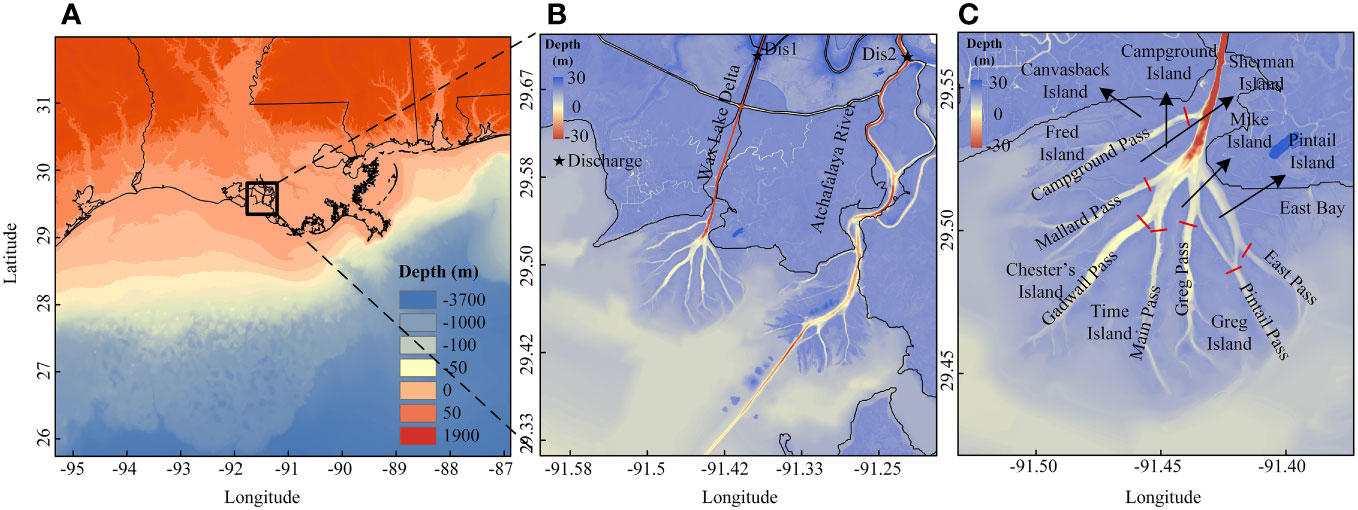
Figure 1 (A) The bathymetry of Louisiana’s coastal zones, the negative values are below mean sea level, (B) The bathymetry of Atchafalaya River and Wax Lake Outlet, and the location of discharge measurement stations (star points), and (C) The names of islands and 7 main channels in the Delta and the cross sections shown in red to analyze the water exchange transport.
This study utilized the Delft3D-FLOW and Delft3D-WAQ PART models to simulate the movement of water and transport processes during the passage of cold fronts. The Delft3D-FLOW model, specifically, was used for hydrodynamic simulations solving the momentum and continuity equations, and computed transport and turbulence. The Delft3D-FLOW model uses the finite difference method on a structured curvilinear grid to solve the Reynolds equations for an incompressible fluid under the shallow water and Boussinesq approximations (Deltares, 2018). The velocity output from Delft3D-FLOW was subsequently used as inputs for the Delft3D-PART module.
A curvilinear orthogonal grid in the horizontal with 10 vertical layers was used, which allowed the bottom and surface boundary layers to have higher vertical resolutions. The computational domain for the study covers the area west of the Mississippi River to eastern Texas, including the Louisiana shelf and coastal waters extending offshore to the shelf-break in the south (Figure 2). The model has 776 x 674 horizontal grid cells with spatial varying resolutions ranging from 30 meters to 1.5 kilometers in the cross-shore direction and from 30 meters to 3.5 kilometers in the alongshore direction. The model grid was designed to encompass the numerous shallow channels and low slope areas in the upper part of the WLD and the Atchafalaya Delta. Delft3D incorporates the wetting and drying algorithm which is applied to simulate the inundation process in the intertidal regions and floodplain. The model simulations used a 6-second time step, as determined through a sensitivity analysis of water level variations. For simplicity, waves were not included in the study. The horizontal eddy viscosity and diffusivity were assumed with 1 m2/s and 10 m2/s, respectively. The bottom roughness was based on the Manning formula with a default coefficient value of 0.023 m-1/3s.
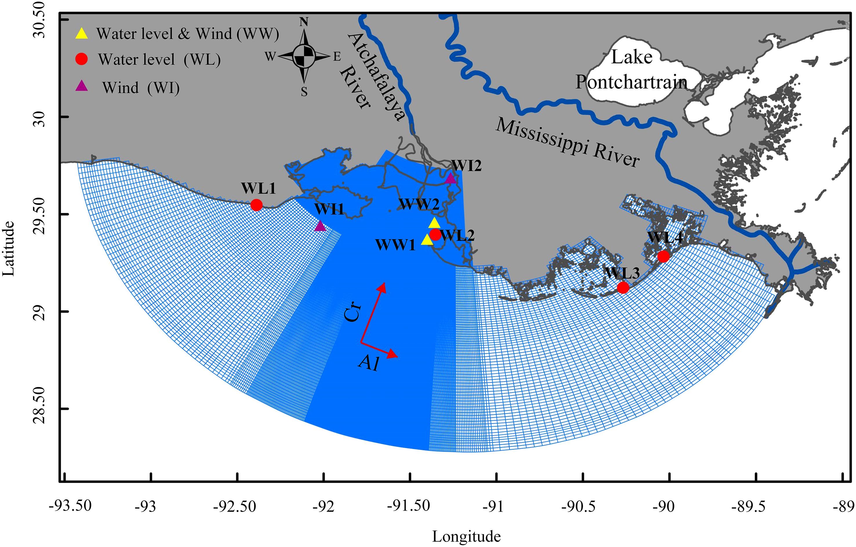
Figure 2 Model grid setup with the location of measuring stations, including wind (WI), water level (WL), and wind & water level (WW) data.
The bathymetry data used in the study for the Atchafalaya/Vermilion Bays and their upper area was obtained through bathymetry surveys conducted in fall 2016 from the NASA Delta-X project (Denbina et al., 2020) and has a resolution of 10 meters. The data was further supplemented with offshore information provided by the National Geophysical Data Center (NGDC) which had a resolution of 90 meters (NGDC, 2001). For the open boundary of the FLOW module, the model used the sea surface elevation with the amplitude and phase of tidal constituents. The tidal constituents included in the model are four diurnal (O1, K1, P1, and Q1) and three semi-diurnal constituents (M2, N2, and S2) along with M4 and M6, which were extracted from the USACE’s East coast 2015 computation done by ADCIRC 2DDI (Szpilka et al., 2018).
The model assigns river discharge for the WLO and Atchafalaya River based on the measurements from the USGS Wax Lake Outlet at Calumet station (USGS 07381590) and Lower Atchafalaya River at Morgan City station (USGS 07381600), respectively. The model uses spatially uniform and temporally variable wind data based on their availability as inputs to incorporate the long-term surface wind forcing. The hourly wind data at WI1 (https://www.wavcis.lsu.edu/) and ones measured every 6 minutes at Eugene Island (WW1), LAWMA (WW2), and Berwick (WW3) and provided by the National Oceanic and Atmospheric Administration (NOAA, 2022), were utilized based on their availability. The power law method is used to convert the wind speeds measured at various elevations above the sea surface to the standard height of 10 meters (U10) above the surface (Kamphuis, 2020).
The model’s ability to simulate water levels was calibrated by comparing the simulated water level with field measurements taken at six stations in January 2020. The model was further verified by comparing the simulation results with observations from September 2021.
To evaluate the accuracy of the water level distribution predicted by the model, it was compared against measurements taken by NOAA at five locations: Eugene Island (WW1), LAWMA (WW2), Freshwater (WL1), Port Fourchon (WL3), Grand Isle (WL4), and another station of USGS at the Mouth of Atchafalaya (WL2) (Figure 2). To assess the model’s performance, the skill score, root mean square error (RMSE), and correlation coefficient were computed.
The skill score, which measures how well the model reproduces the observations, was formulated as (Willmott, 1981),
where and are the predicted and observed values, respectively, is the mean observed value, and is the total number of data points.
The root mean squared error () was outlined as:
The Pearson correlation coefficient which is a measure of the linear correlation between observed and modeled data, was defined as (Pearson, 1895):
where is the mean predicted value.
The skill scores are between 0.75 and 0.86 (Table 1), indicating that the simulated water levels generally agree with the observed water levels, as confirmed by the RMSE, and correlation coefficient, when compared to other studies (e.g., Payandeh et al., 2019; Feizabadi et al., 2022). More specially, the skill score calculated for September 2021 during the validation period is in a higher range between 0.85 and 0.92.
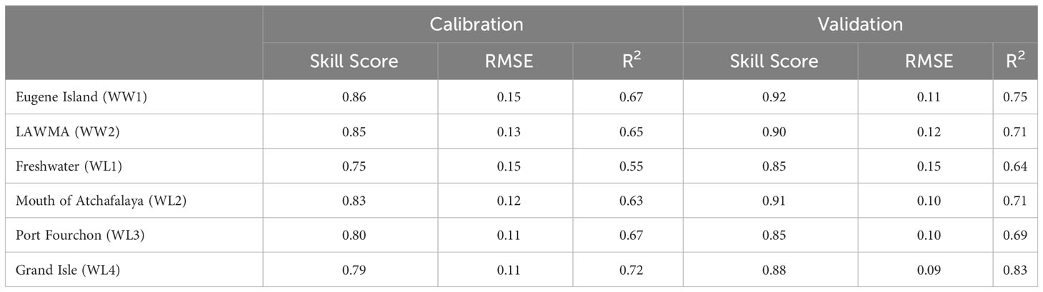
Table 1 Statistics of the model-data comparison in water elevation (m).
The comparison of the simulated water level time series with the field measurements at stations WW1, WW2, WL2, and WL4 (Figure 3) for the period for January 2020 and September 2021, suggests that the model’s accuracy is satisfactory for further application in the proposed studies.
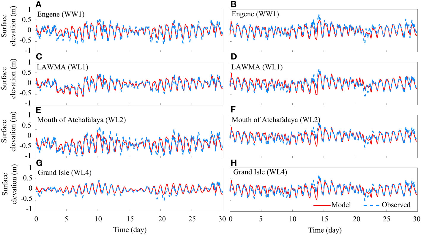
Figure 3 Modeled and measured water level elevation at Eugene (A, B), LAWMA (C, D), Mouth of Atchafalaya (E, F), and Grand Isle (G, H) stations. The left and right panels correspond to the calibration (January 2020) and validation (September 2021), respectively.
The Wax Lake Delta is characterized by a complex network of channels that transport water through the delta, including seven main channels (Figure 1B). The water circulation and flux in the WLD is mainly influenced by the channel network’s configuration and its connection to the inundated islands (Hiatt and Passalacqua, 2017; Olliver and Edmonds, 2021).
To calculate the net water flux in each channel, we established cross-sections spanning the channel using bathymetry to identify mean flow directions and bank locations. The water transport at an individual cross-section is calculated using the following equation:
where is the horizontal velocity component perpendicular to the cross-section.
The water depth is represented by H, is the surface elevation, and L is the width of the cross-section. The initial time is denoted by t1, while the final time is t2. To determine subtidal water volume transport, a sixth order Butterworth low-pass filter with a cutoff frequency of 0.6 cycles per day is utilized. The average contribution of channels in transporting water was calculated for a one -day period before and after a cold front passing the WLD region.
To investigate the proportion of water transported through various sides of the WLD, the water transport was separated into three categories: the western channels (comprising of Campground Pass, Mallard Pass and Gadwall Pass), the central channels (the Main Pass and Greg Pass) and the eastern channels (the Pintail Pass and East Pass).
In addition to the numerical simulations, we also applied an analytical model to evaluate the impact of both remote and local forces on water level fluctuations in an idealized bay. This is based on the model of Garvine (1985) developed for a simple barotropic wind-driven oscillation in an idealized estuary. It considers the effect of both remote and local wind effects on estuarine subtidal fluctuations by a rectilinear wind varying in two opposite directions. Feng and Li (2010) made modifications to Garvine’s model to incorporate a cold front wind that rotates in the clockwise direction. The analytic solution of the water level under rotary wind can be written as:
The model uses various variables to describe the relationship between remote and local forces of wind and the water level variability in the estuary. Here represents the length of the estuary, is a coefficient that relates the subtidal water level to cross-shelf Ekman flow, is the initial phase, is the angular velocity of wind, is the linear shallow water wave propagation speed in a water with a constant depth of , is the water density, is the Coriolis parameter, and τ is the wind stress, which is calculated using the quadratic law,
where the density of air takes a value of 1.3 kg/m3, U10 is wind velocity magnitude at 10 m above sea level and drag coefficient, , is evaluated by using the empirical formula proposed by Wu (Wu, 1980; Wu, 1994).
The default values for the empirical factors in the formula proposed by Wu (Wu, 1980; Wu, 1994) were = 1.255 × 10⁻³, = 2.425 × 10⁻³, = 7 m/s, and = 25 m/s. The wind stress was decomposed to the alongshore and cross-shore components (Figure 2). The axis of Atchafalaya/Vermilion Bays are tilted ~24° clockwise from the north latitudinal line, and the cross-shore axis relative to the coastline is ~90° therefore the cross-shore winds (~24°) give the local wind effect and the alongshore winds (~114° clockwise from the true north) produce the remote wind effect, as treated in Garvine (1985). For simplicity the analytical model domain is a 50-km wide rectangular estuary with a 20-km long continental shelf, which captures the basic geometry of the modeling domain near the WLD.
In equation (5), “ “ is a complex wave number of order unity, which is represented by the given formula,
where is a dimensionless parameter, is the root mean square subtidal current, is the bottom drag coefficient, and h is the mean water depth. The equation (5) provides both the impact of remote and local winds on water level fluctuations. The cosh function, which is linked to the coefficient α, illustrates the water level changes resulting from remote winds, while the sinh term represents water level changes resulting from local winds. These two effects are shown separately in equations (10) and (11).
The average depth of the Atchafalaya/Vermilion Bays is 2.2 meters. The Coriolis parameter was defined as 7.18 × 10⁻⁵ s−1 corresponding to a latitude of 29.5°N. A bottom drag coefficient of 5.0 × 10⁻³ Li (2003) and a root mean square subtidal current of 0.1 m/s were utilized to estimate the dimensionless bottom friction parameter λ, which was calculated to be 11.4. The density of seawater used in the calculation was 1,027 kg/m3. The remote wind coefficient, α, varies based on both the physical characteristics of the bay and offshore shelf morphology. Garvine (1985) estimated α to be 5×10⁻⁴ m2·s·kg−1 for the Chesapeake Bay and Delaware Estuary, but this value is not suitable for the Atchafalaya/Vermilion Bays as its depth is much shallower and the basin geometry is different. The frictional damping effect becomes more significant in shallow Louisiana estuaries, leading to a much lower expected value of α compared to Chesapeake Bay and Delaware Estuary (∼10 m). Feng and Li (2010) found a value of 8×10⁻⁵ m2·s·kg−1 to be the best fit for observational data in the region, and that value was used in the present study.
The D-WAQ PART model (3D) is employed to examine the particle transport routes that occur during the passage of cold fronts. The model utilizes a random-walk approach, as it involves a limited number of particles, and the simulated behavior is stochastic in nature (Rubinstein, 1981). The model follows the movement of individual particles using the Lagrangian description (Wilson and Sawford, 1996). When a particle is present in a flow field with Eulerian velocities, its velocity can be divided into two parts: a resolved part and a sub-grid part . The resolved part U is spatially resolved and can be computed explicitly, whereas the sub-grid part is a smaller-scale velocity component that cannot be directly resolved. The total displacement of a particle in the flow field is obtained by integrating both the resolved and sub-grid parts of the velocity.
If the time step is sufficiently large such that the particle’s previous velocity becomes negligible, a zero-order model may be employed. A zero-order model assumes that the velocity of the particle is constant over the time step and is given by the Eulerian velocity at the particle’s current location.
The random displacement of a particle over the time step is represented by the variable R, which is influenced by the diffusion coefficient D and follows the standard Gaussian distribution G(0, 1). The zero-order model, along with the numerical scheme, forms the fundamental components of the particle D-WAQ PART model.
In a 3D simulation, a point source situated 2 km from the intersection of WLO and Campground Pass (29.559 N, 91.423 W) was used to release ten neutrally buoyant particles simultaneously on the water surface. It is important to note that these particles were programmed in the simulation to neither stick to the land boundary nor settle down. The particle tracking model has the flexibility to use either the saved model time step or a chosen multiple sub-model time steps to move particles through the model domain. The model tracks and stores the location and time of particles at each time step, and in this study, particle positions are saved every 10 minutes.
Nine cold front events passing the WLD region were examined and for each case the moving direction of the front orientation and wind magnitude were identified (Table 2). The timing of the cold fronts, as shown in Table 2, were established by identifying when the cold front entered and left the state of Louisiana using the 3-hourly surface analysis maps from NOAA’s Hydrometeorological Prediction Center (HPC, 2023). For the scenarios that fall beyond the calibration and validation time periods, separate simulations were carried out for a duration of one month to guarantee proper representation of circulation patterns in the main domain. The differences in error indexes between these simulations and the validation simulation from the mentioned stations were found to be less than 13%.
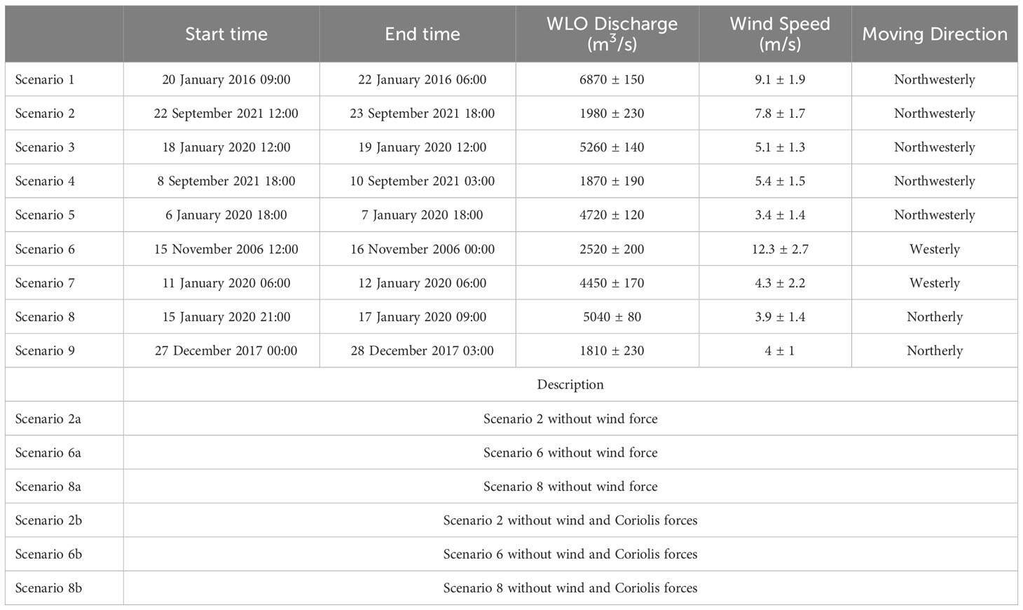
Table 2 Summary of cold fronts scenarios for model simulations.
To help the discussion on the effect of different cold fronts, we define the cold front moving direction to be the direction along which the cold front is coming from, which is roughly perpendicular to the front orientation. Orientation refers to the spatial configuration of the cold front that represents the line or boundary that separates the advancing cold air mass from the displaced warmer air mass. To assess the effect of cold front moving direction on hydrodynamic conditions in the WLD, the moving direction was classified into three categories: northerly, westerly, and northwesterly. The results of the simulation are discussed and presented in the following sections.
In Figure 4, the red bars demonstrate the average contribution of channels in transporting water to the Atchafalaya Bay in nine scenarios during both pre-frontal and post-frontal phases. The results of the study indicate that the Gadwall Pass is the most significant in terms of water transport, accounting for approximately 26.7% of the total, followed by the Greg Pass, which accounts for 18.1%. Meanwhile, the East Pass and Pintail Pass have the lowest contribution to water transport, at about 5.7% and 10.3%, respectively.
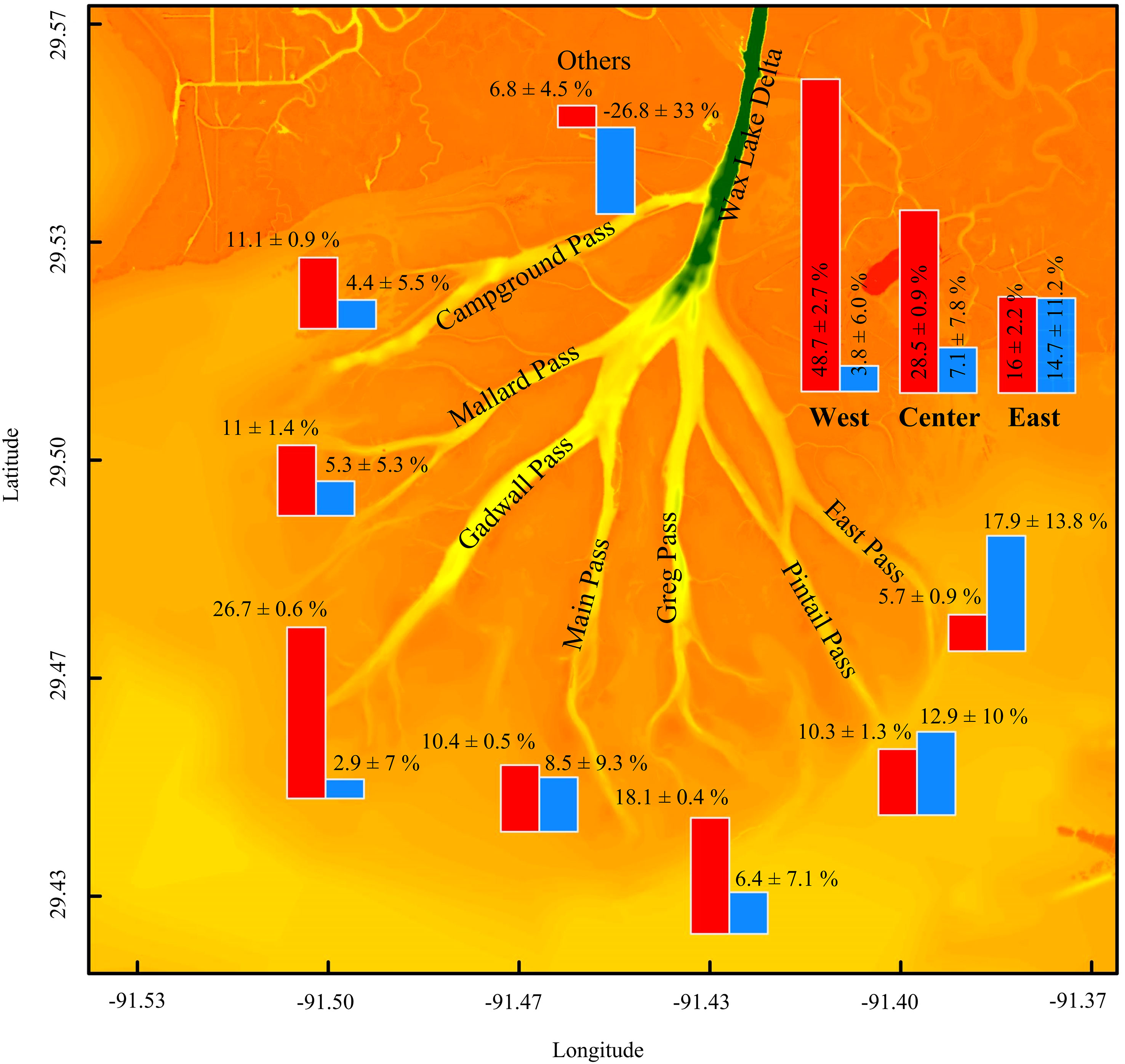
Figure 4 The average percentage contribution of water exchangeand the average percentage changes during the passage of cold fronts in the channels. The red bars represent the average percentage contributions for a one-day period before and after the cold front passage, while the blue bars represent the average changes in water volume transport within the channels during the passage of a cold front compared to a one-day period before. The caption for the “Others” presents the quantities of water transported through secondary channels and the intrusion into wetlands.
Results show that about 48.7% of the water transport takes place through western channels and 28.5% through central channels, while the eastern channels have the lowest contribution at about 16%. Additionally, a considerable percentage of water, around 6.8%, flows through secondary channels or going through the wetlands between the channels (Figure 4) as also found in Zhang et al. (2022). However, the quantification of water flow through these secondary channels or wetlands depends greatly on the location of cross sections chosen for transport computation. Previous studies placed cross sections at the end of channels, whereas in this study, the cross sections were positioned immediately after channel branching to determine the average contribution of each channel to water transport (shown in Figure 1C).
The blue bars in Figure 4 indicate the average changes in water volume transport within channels during the passage of a cold front compared to the pre-frontal phase cross nine scenarios. The western channels exhibit the least changes in water volume transport, averaging around 3.8%, in stark contrast to the eastern channels, which experience an average change of about 14.7%. As for the central channels, there is an increase of approximately 7.1% in water volume transport. The significant rise in water volume transport within the eastern channels during cold front passage indicates an increase in the contribution of transport through these channels. This should have an impact on the sediment transport and wetland habitats in the WLD. Additionally, it can be observed that cold fronts decrease the amount of water transported through secondary channels and the intrusion into wetlands by about 26.8%. During passing cold fronts, as the water level and depth decrease, part of the island may be exposed in the air and the water is more likely to flow out of the main channels than over the shallow water because the shallow waters can become dry temporarily.
Table 3 demonstrates the variations in water volume transport during a cold front by contrasting the water transport before and after a cold front for Scenarios 2, 6, 8, and 9. In Scenario 2, which is a northwesterly cold front, the data reveals that it has a significant impact on eastern channels, resulting in a 27% increase in water transport, in contrast to the western (0.1%) and central channels (4.1%). The greatest variations in water transport in the major channels occur in Scenario 6, which is a westerly cold front. The eastern channels experience a 34.9% enhancement in water transport, which is equivalent to 143 (m3/s), whereas the water transport in western channels decreases about 2%, equivalent to 28 (m3/s). In Scenarios 8 and 9, both are northerly cold fronts, the response of water transport in the main channels to the cold front is consistent with the response of water transport in the WLO discharge (Table 3). In other words, the primary effect of a northerly cold front is on the transport in the WLO, especially during low discharge. Comparing Scenarios 8 and 9, the wind velocity is comparable but the WLO discharge during Scenario 9 is 1810 m3/s, which is about 36% of the discharge in Scenario 8 (Table 2). Therefore, the changes during Scenario 9 are more significant. It can be deduced that the effects of a passing cold front are more pronounced during the dry season when the WLO discharge is low.
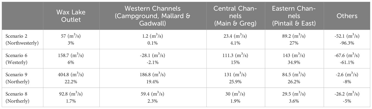
Table 3 The effect of passing cold fronts on volume of water transport through main channels and other paths for Scenarios 2, 6, 9, and 8.
The results indicate that a passing cold front causes an increase in the discharge of the WLO due to the effect of wind stress. For instance, the WLO discharge increases by about 22%, equivalent to 405 (m3/s), during Scenario 9 (Table 3). Furthermore, the amount of water transported through secondary channels and the intrusion into wetlands decreases when cold fronts with any moving direction pass through. The most substantial decrease in other transport can be observed in Scenarios 2 and 6, with reductions of - 96% and - 61%, respectively.
To quantify spatial variability of water level fluctuations in response to cold front passage, the difference between low-pass filtered water level variation (setup and set down) has been calculated for each scenario at the WLD (Figures 5, 6). A sixth order Butterworth low-pass filter with a cutoff frequency of 0.6 cycles per day is applied to determine subtidal fluctuations of water levels and currents. Subsequently, the disparity between the subtidal water level escalation prompted by pre-frontal winds originating from the southern quadrants, and the subsequent subtidal water level reduction arising from the reversed winds during the post-frontal phase is quantified. As highlighted in the research conducted by Li et al. (2018), the subtidal water level undergoes fluctuation in response to the passage of cold fronts, exhibiting a characteristic pattern akin to the shape of the letter “M”.
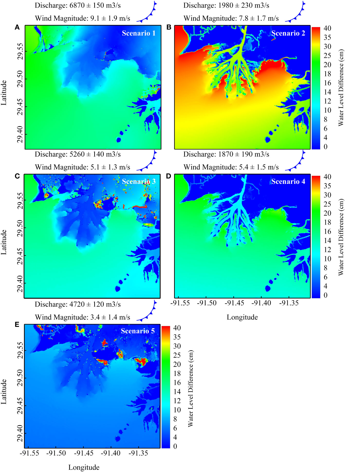
Figure 5 The subtidal water level fluctuations due to cold fronts from the northwest (A–E) in Wax Lake delta and Atchafalaya Bay. The Water Level Difference refers to the disparity between the rise in subtidal water level before cold front (pre-frontal) and the decrease in subtidal water level after cold front (post-frontal).
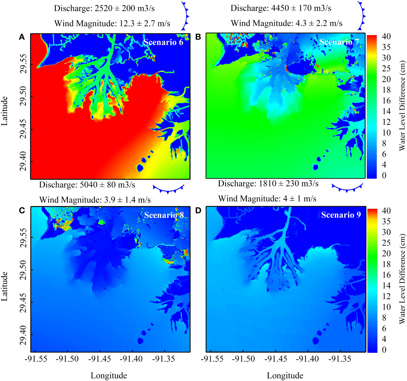
Figure 6 The subtidal water level fluctuations due to cold fronts from the west (A, B) and those from the north (C, D) in Wax Lake delta and Atchafalaya Bay. The Water Level Difference refers to the disparity between the rise in subtidal water level before cold front (pre-frontal) and the decrease in subtidal water level before cold front (post-frontal).
The maximum subtidal water level fluctuations caused by passing northwesterly cold fronts in the WLD and Atchafalaya Bay occur in Canvasback Bay, Fred Island, Tim Island, Mike Island, Greg Island, and East Bay (Figure 5). However, the magnitude of changes depends on the wind magnitude and river discharge. For example, the subtidal water level variation in the Tim and Greg Islands during a northwesterly cold front with an average wind magnitude of 9.1 m/s and average WLO discharge of 6870 m3/s is roughly 15 cm (Scenario 1), while in Scenario 2, with the lower wind magnitude of 7.8 m/s and a lower river discharge of 1980 m3/s, the subtidal water level variation increases to 45 cm (Figures 5A, B). The results also indicate the significance of wind magnitude on the subtidal water level variation. It is shown that when the average wind speed increases from 5.4 m/s to 7.8 m/s with an approximately constant river discharge of around 1900 m3/s, the subtidal water level variation doubles (Figures 5B, D).
Comparison of Figures 5C, D shows that under approximately the same average wind speed, the subtidal water level fluctuations in the WLD and Atchafalaya Bay are greater when the river discharge is lower, this agrees with the comparison of Scenarios 8 and 9 during northerly cold fronts (Figures 6C, D). However, a high WLO discharge can cause water intrusion in the delta islands and coastal plain marsh upstream of the WLD. This means that when the river discharge is higher, the passing of a cold front causes the water level variation to be affected in a wider area but with a smaller magnitude. So, the effects of passing cold fronts with different moving directions on water level fluctuation in the WLD and Atchafalaya Bay are largely dependent on the river discharge. The impact is more significant when the river discharge is lower, which is associated with smaller water depth and thus higher nonlinearity. In the context of hydrodynamics, nonlinearity is often measured by parameters such as wave height or water level variations relative to water depth (ζ/h). A higher value of these parameters signifies a stronger nonlinear effect, leading to the generation of subtidal and over-tidal components of oscillations and flows (Li and O’Donnell, 1997; Pihl et al., 2001). Furthermore, within shallow-water regions, the gradient of water level is directly proportional to the wind stress divided by the water depth. Therefore, a decrease in water depth results in an amplified variation in water level. In Scenario 5, the water level variation is less severe than in Scenario 3, despite a 10% decrease in WLO discharge, due to a decrease of approximately 33% in wind speed (Figure 5E). Results for northwesterly scenarios illustrate that the water level variation in the WLD is controlled by both the WLO discharge and wind magnitude.
The effect of the direction of cold fronts on changes in water levels is shown by the subtidal water level response to westerly and northerly cold fronts under different average wind speeds and discharge rates (Figure 6). The westerly cold fronts lead to substantial changes in water levels in Canvasback Bay, Fred Island, Tim Island, Mike Island, Greg Island, and East Bay (Figures 6A, B). In Scenario 6, an eastward cold front with an average wind speed of 12.3 m/s can result in a water level variation of approximately 0.45 m in the islands (such as Mike and Tim islands) and 0.65 m in the East Bay, when the average discharge rate from the outlet is 2520 m3/s. Figures 6C, D show that northerly cold fronts cause the lowest water level variations in the WLD and Atchafalaya Bay compared to the other directions. For example, in Scenario 9 (Figure 6D), the water level variations in different regions range from 0 to 0.1 m, while in Scenario 7 (Figure 6B), which has the same average wind speed but a higher discharge, the variations range from 0 to 0.25 m. These results imply that the cold front direction can be a factor influencing the flow field and transport in the delta region.
The larger water level fluctuations in all scenarios in Canvasback Bay, Fred Island, Tim Island, Mike Island, Greg Island, and East Bay relative to Atchafalaya Bay can be attributed to the impact of local wind stress. Local wind stress over the bay surface can create a water level gradient, with the highest water level variations in the downwind end of the bay. In contrast, water level variations farther away from the downwind end in the bay have smaller magnitude by the local wind effect because the fetch is shorter.
In Scenario 7 (Figure 6B), the water level difference is greater than that in Scenario 4 (Figure 5D) despite a higher discharge and lower average wind speed. Scenarios 7 and 9 have similar average wind speeds but the outlet discharge is lower in Scenario 9, and the water level variation caused by the westerly cold front in Scenario 7 is more significant. The results reveal that the water level fluctuations caused by westerly cold fronts are more substantial as compared to those caused by the northwesterly and northerly cold fronts.
The pattern of water circulation determines how sediment and nutrients are transported and distributed in a delta. As water flows within the delta, it transports sediment that can settle in various locations, shaped by factors including water flow direction, strength of flow, and the shape of the delta’s bed (Roberts et al., 2015; Wagner and Mohrig, 2019).
Figure 7 illustrates the response of average surface water circulation to northwesterly cold fronts for a one-day period before and after the passage. Despite the cold front having a strong average speed of 9.1 m/s, Figures 7A, B show that its effect on the current speed and streamline pattern is limited because of the prevailing discharge of 6870 m3/s from the WLO in Scenario 1. In this scenario, water exits Atchafalaya Bay heading southwest with the average surface subtidal current in the Gadwall Pass and other passes reaching 1.5 m/s and 0.8 m/s, respectively. In Scenarios 2 and 4, the low WLO discharge results in weak subtidal currents, with magnitudes of 0.45 m/s in the channels and 0.25 m/s in Atchafalaya the Bay. However, the response of the streamline pattern to the passing cold front is different in these two scenarios. In Scenario 2, the streamlines in Atchafalaya Bay are directed westward before the cold front due to a strong southerly wind, causing a change in the streamlines from southwest to northwest (as seen in Figure 7C). In other words, the wind force is not strong enough to cause the streamlines to flow towards the north, nor is the outflow momentum from the WLO sufficient to change the flow direction to the southwest. Figure 7C displays the discharge patterns of water from central channels (the Main Pass and Greg Pass) and eastern channels (the Pintail Pass and East Pass) into the adjacent islands, such as the Tim, Mike, and Greg Islands, while water exiting from the western channels (Campground Pass, Mallard Pass, and Gadwall Pass) move towards the western side. The alterations in the flow pattern of streamlines can result in changes in sediment deposition on the islands. Once the cold front is passed, strong northwesterly winds drive the subtidal current towards the southeast direction, resulting in a noticeable shift in the pattern of streamlines (as shown in Figure 7D). Scenario 3 highlights the effect of a cold front on the subtidal currents in the channels and the Atchafalaya Bay, which results in an increase in the subtidal currents but with minimal changes in the direction of the streamlines (Figures 7E, F). The cold front has caused a significant increase (almost doubled) in the subtidal currents, in a vast area of the Atchafalaya Bay. In comparison to the earlier scenarios, the wind force significantly overpowers the WLO outflow momentum due to the low discharge in Scenario 4 (Figures 7G). This leads to a change in the direction of the subtidal current in the Atchafalaya Bay, shifting from northward prior to the cold front to southward during the cold front’s passage, affecting the transport process in the channels and shoals (Figures 7G, H). The magnitude and streamlines of subtidal currents remain mostly unchanged in scenario 5 because of the high WLO discharge and weak average wind (not shown).
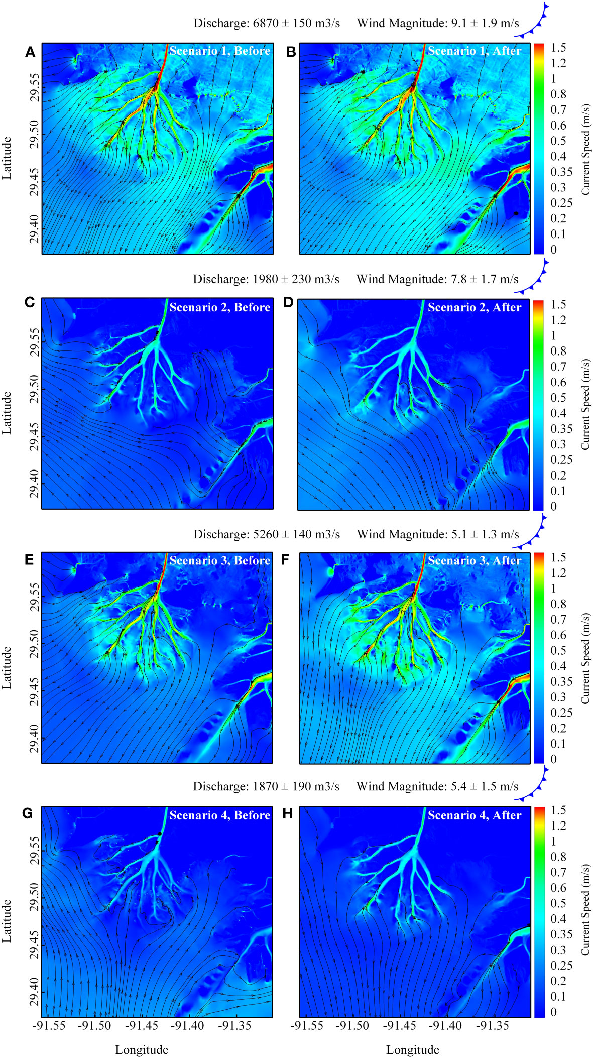
Figure 7 The average surface water circulation one day prior to (pre-frontal, left) and one day after (post-frontal, right) the arrival of a cold front from the northwest (A–H).
Figure 8 shows the response of average surface subtidal current to passing westerly and northerly cold fronts. A comparison of Figures 8A, B reveals that the strong cold front with an average wind speed of 12.3 m/s causes the streamlines to shift towards the south when the WLO discharge is around 2520 m3/s, but there is only a limited change in the magnitude of subtidal currents (Scenario 6). Despite the powerful westerly wind force, the streamlines are not altered to the east, indicating that the force is insufficient to cause such a change in direction. In Scenario 7, the higher subtidal westward flow prior to the cold front is primarily attributed to the wind from the east (Figure 8C). Once the cold front arrives, the strong westerly winds are potent enough to shift the streamlines to the southwest. Results show that the arrival of a westerly cold front leads to an increase in subtidal currents in all channels, with the eastern channels being particularly affected. Since the westerly cold front pushes the water in the WLO and delta to exit more prominently from the eastern channel, as discussed in section 4.1. As an example, in Scenario 6, the subtidal current in the center of the Pintail channel saw a substantial increase of 30%.
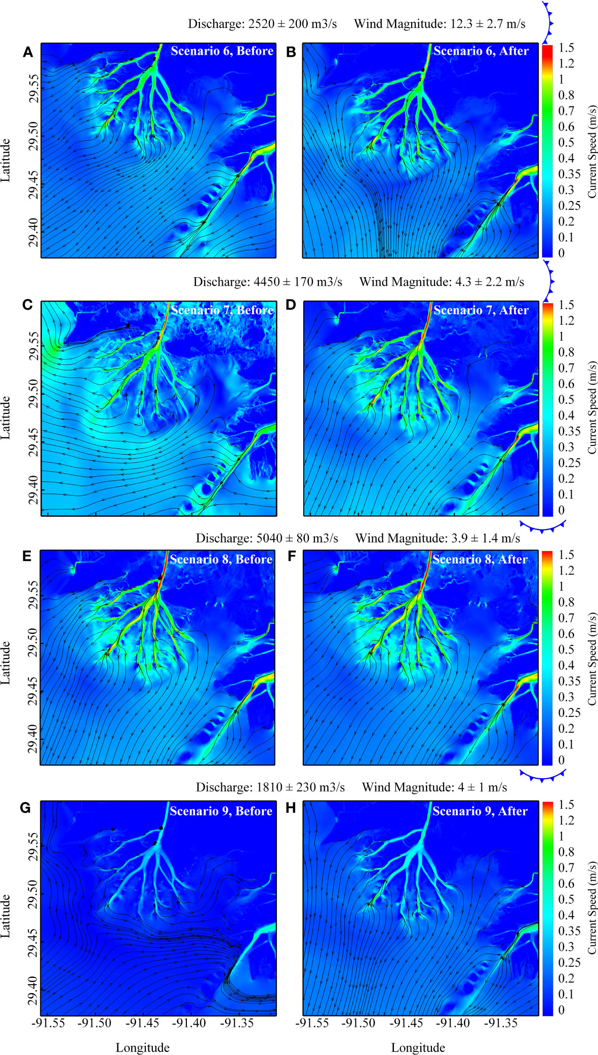
Figure 8 The average surface water circulation one day prior to (pre-frontal, left) and one day after (post-frontal, right) the arrival of a cold front from the west (A–D) and north (E–H).
The presence of a northerly cold front with an average wind speed of 3.9 m/s (Figures 8E, F), does not bring about any significant changes in the streamline pattern and subtidal current when the WLO discharge is at a level of 5040 m3/s. In contrast, when the wind speed is similar to Scenario 8, but the discharge is reduced to 1810 m3/s, the flow direction of the streamlines is impacted (Figure 8G). As shown in Figure 8G, the streamlines show flows toward the northeast instead of southwest before the cold front, due to the decreased outflow momentum from the WLO in comparison to the southerly wind force in Scenario 9. Thus, instead of flowing out to the continental shelf, the water leaving the main channels is directed towards the adjacent islands or shallow waters and landward regions of the system. Following the passage of the northerly cold front, the streamlines shift in the southwest direction (Figure 8H). The changes in the magnitude of the surface current are consistent with the variation of water volume transport during the passing cold front. In the post-frontal phase, as the wind force drives the flow from the channel towards the bay and enhances the intensity of the surface current, there is an increase in water volume transport compared to the pre-frontal phase.
Overall, the passage of a cold front leads to major changes in the streamline patterns and subtidal currents of the WLD and Atchafalaya Bay, particularly during low WLO discharge. Based on the streamline patterns, it can be inferred that passing a cold front during a low WLO discharge may cause a greater amount of nutrient and sediment-rich water being transported from the primary channels to the shallow waters where they may remain there for a longer period than under normal circumstances.
The results presented in Section 4 demonstrate that the passage of a cold front has a significant impact on the hydrodynamics, including water volume transport, water level, and horizontal water circulation, in the WLD, based on the strengthen and direction of cold front, as well as the WLO discharge. Because the WLD is a complex delta system with multiple channels, the transport patterns and water level variations have significant implications for nutrient removal, sediment deposition, wetland habitats, and delta evolution. Given the significance of water level variations in the WLD, an analytical model was used to evaluate the drivers of water level fluctuation during the passage of a cold front. Additionally, particle tracking was utilized to assess the impact of these changes on the transport processes within the channels and Atchafalaya Bay.
Figure 9A displays the measured wind data from September 21, 2021, at 00:00 to September 25, 2021, at 04:00. Figure 9B displays an analytical model-generated representation of a cold front wind, with a constant wind speed of 8 m/s. According to the period of cold front (100h), the angular frequency of the wind was determined to be 1.75 × 10⁻⁵ s-1. In the equation (6) (Wu, 1980; Wu, 1994), the surface drag coefficient was set to 1.32*10-3. Figure 9C illustrates typical observed water level variations during a cold front event (Scenario 2) at the LAWMA station (∼15 km from mouth). Meanwhile, Figure 9D shows the model-predicted water level variation, which is generally consistent with the observed results. The amplitude of water level induced by cross-shore wind forcing (0.08 m) is smaller than that from alongshore wind forcing (0.15 m) (Figure 9D).
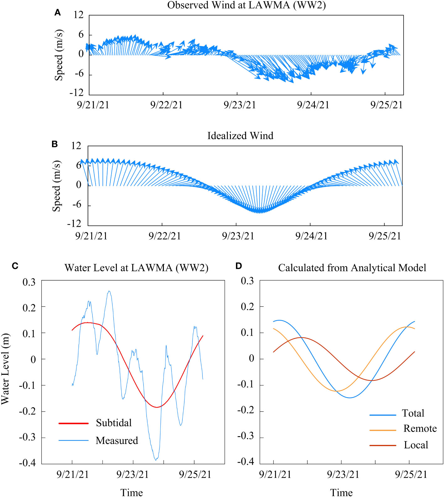
Figure 9 (A) Wind measurement at LAWMA station from September 21, 2021, at 00:00 to September 25, 2021, at 04:00, (B) Idealized clockwise rotating wind with 100 hour-period, (C) measured and subtidal water level at LAWMA, (D) The yellow and red lines demonstrate water level variations induced by cross-shore winds and alongshore winds, respectively and blue line is the total water level.
The analytical model with rotary wind (Feng and Li, 2010) was examined to determine the water level variation in various water depths and locations as well as both remote and local wind effects during the same cold front event (Figure 10). For a complete description, we reiterate the findings of Feng and Li (2010) on the remote and local wind effects, before we look at the effect of overall water depth changes at low and high discharge conditions. The first row of figures shows water level fluctuation caused by local and remote wind effects as a function of distance from the mouth of the bay (Figures 10A-C). Results show that the remote wind-induced fluctuations are not dependent on the distance from the mouth and remain constant throughout the bay, consistent with Feng and Li (2010). The uniformity of remote wind-induced water level fluctuations along the bay is a result of the short length of the bay compared to the wavelength and the remote-wind-induced motion behaves as a standing wave (Honda et al., 1908). Therefore, this behavior of remote wind-induced water level fluctuations explains the higher water level variations in the WLD and Atchafalaya Bay during westerly cold fronts compared to the northwesterly and northerly cold fronts. Additionally, the analysis shows that the water level slope is mainly influenced by local wind forcing (Figures 10A–C), consistent with Garvine (1985) and other more recent studies. This means that the effects of local winds on water level variation are more pronounced at the head of the bay than at the mouth during a cold front, which explains the higher water level fluctuations observed in areas such as East Bay, Fred Island, and other islands during a cold front event.
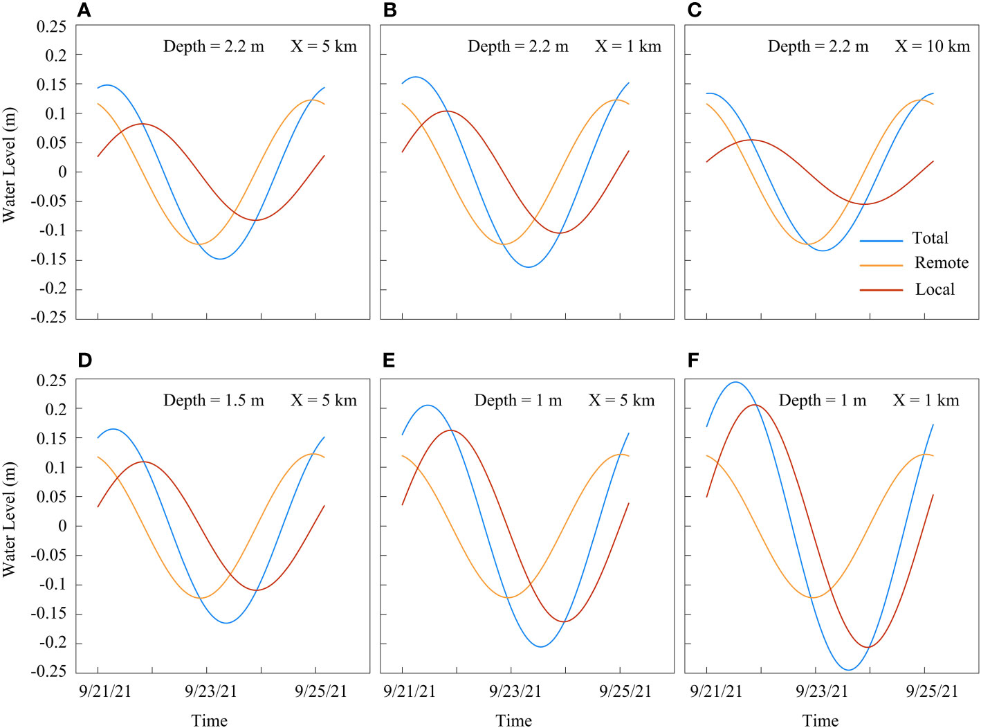
Figure 10 The response of water level variation to the local and remote winds based on the analytical model in different average water depths and distances from head of the bay. (A) water depth of 2.2 m and 5 km distance, (B) water depth of 2.2 m and 1 km distance, (C) water depth of 2.2 m and 10 km distance, (D) water depth of 1.5 m and 5 km distance, (E) water depth of 1m and 5 km distance, (F) water depth of 1m and 1 km distance. The yellow and red lines demonstrate water level variations induced by cross-shore winds and alongshore winds, respectively, and the blue line is the total water level.
Figures 10A, D, E show that water level changes caused by local wind increase significantly as the water depth decreases, while those caused by remote wind remain constant. For example, when the water depth decreases from 2.2 to 1 m, the amplitude of water level fluctuations induced by local wind at the LAWMA station, located 5 km from the bay head, increases by approximately 0.08 m (Figure 10E). The impact of a decrease in water depth on water level fluctuations caused by local wind becomes more pronounced in the low-lying areas near the head of the bay. The analytical model demonstrates that when the water depth is 1 m, the water level changes caused by local wind increase by approximately 0.1 m in areas located 1 km from the head of the bay (Figure 10F). The results from the analytical model indicate that the increased water level variations in low-lying areas during cold fronts with low WLO discharge can be attributed to the decrease in water depth. For instance, in Scenario 3 with an average WLO flow rate of 5260 m3/s, the estimated water depth at the LAWMA station is 1.05 m, which decreases to 0.82 m when the flow rate decreases to 1870 m3/s in Scenario 4.
To explore the influence of passing cold fronts under various conditions and the significance of the Coriolis force on water transport, a Lagrangian particle tracking model was utilized. The particle trajectory may imply the trajectory of suspended materials such as sediment and nutrients. However, it’s worth noting that predicting the fate of suspended sediment and nutrients is more intricate than simply tracking particles. This is because the particles in this study are buoyant and passive, while the transport of suspended sediment and nutrients involves complex physical and biogeochemical processes. The simulation involved releasing particles 2 km from the intersection of the WLO and Campground Pass, and then observing their movements after the arrival of cold fronts. The path of the particles was determined based on the majority behavior of the particles, which was tracked for a period of 8 days (Figure 11, Lagrangian particle tracks shown as colored lines).
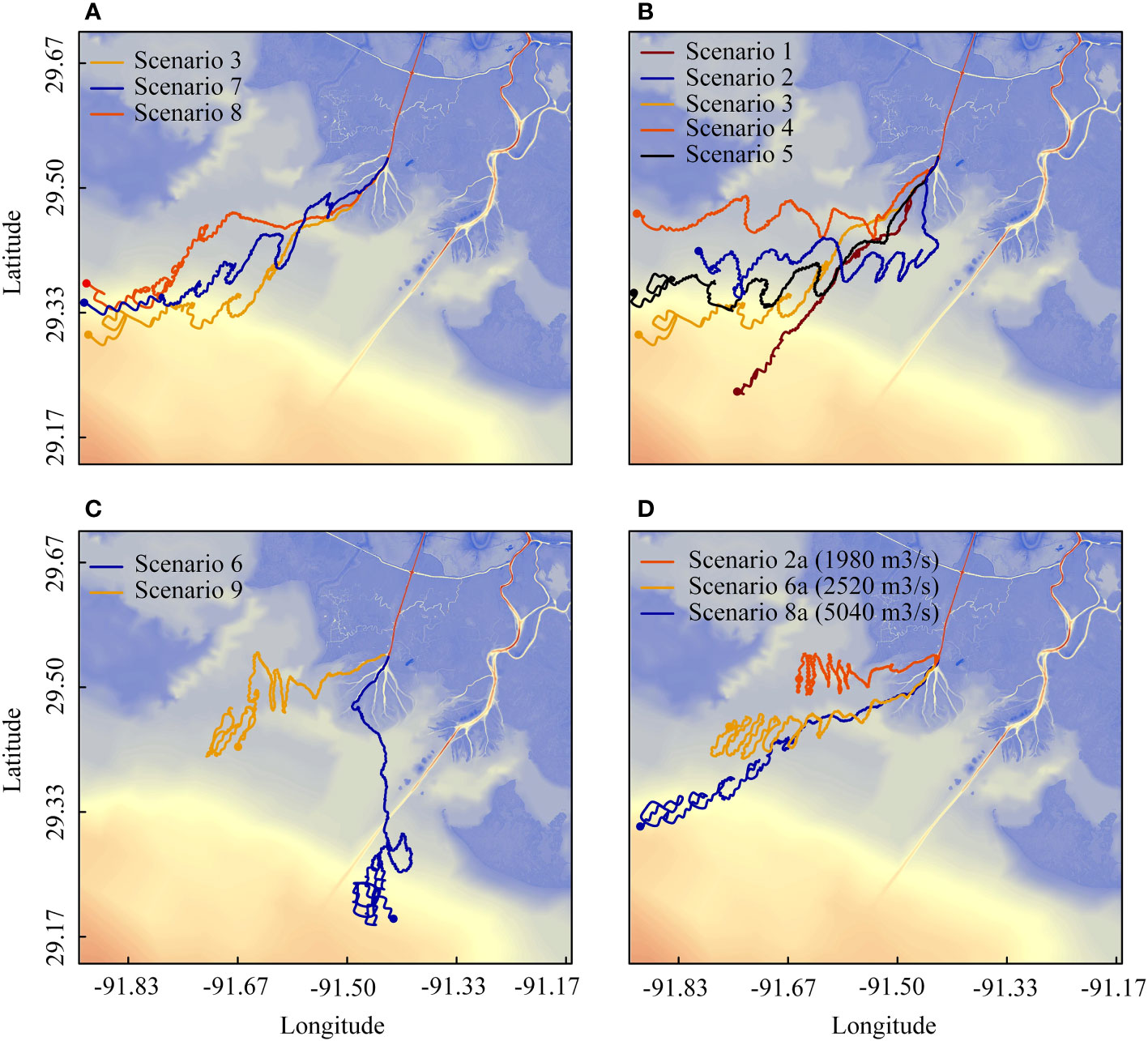
Figure 11 Trajectory of particles using a LAgrangian model for 8 days. (A) Trajectory of particles during Scenarios 3, 7, and 8, (B) Trajectory of particles during northwesterly cold fronts, (C) Trajectory of particles during Scenarios 6 and 9, (D) Trajectory of particles during scenarios 2, 6, and 8 without wind force.
Figure 11A displays the paths of particles in Scenarios 3, 7, and 8 with different moving directions of the cold fronts, but roughly the same WLO discharge (about 5000 m3/s) and wind magnitude (4-5 m/s). The results indicate that under these conditions, there is no significant difference between scenarios. The majority of particles flow out from Gadwall Pass and are influenced by tidal currents based on the outflow momentum, ultimately being deflected to the west side likely due to the Coriolis effect (Kourafalou et al., 1996). The impact of changes in WLO discharge and wind magnitude on the particle tracking under northwesterly cold fronts is depicted in Figure 11B. As seen in Scenario 1, with a high WLO discharge, the flow carries the particles out of Gadwall Pass and onto the shelf without being impacted by the tidal currents in the Atchafalaya Bay, in contrast to the other scenarios. In Scenario 2, the particles are influenced primarily by the wind force, which overpowers the outflow momentum and other forces. As a result, the particles are pushed to the east and leave the area through the Main Pass. A comparison between Scenarios 3, 4, and 5 reveals that the exit of particles through the Mallard Pass in Scenario 4 is likely caused by the Coriolis force, because the WLO discharge in Scenario 4 is lower when compared to the discharge in Scenarios 3 and 5. In Scenario 6, which features a strong westerly cold front with an average wind speed of 12.3 m/s and WLO discharge of about 2520 m3/s, the wind stress dominates the particle pathway, causing the particles to exit the Gadwall Pass and move towards the east side (Figure 11C). A weak northerly cold front and weak WLO discharge led to the majority of particles exiting from the Campground Pass and remaining in the Atchafalaya Bay after 8 days of tracking (Scenario 9, Figure 11C). This highlights the importance of the moving direction of the cold front in transporting suspended sediment and nutrients, especially in low discharge conditions, as evidenced by the comparison of Scenarios 4 and 9.
Based on the results demonstrated in these scenarios, the WLO discharge is one of the most important factors to determine the trajectory of particles. To highlight the significance of the WLO discharge, particle tracking simulations were conducted for Scenarios 2, 6, and 8, which represent low, moderate, and high WLO discharge, respectively. Wind force was not taken into account in the simulations for these scenarios and were designated as Scenarios 2a, 6a, and 8a (Figure 11D). The results of the simulations indicate that under low WLO discharge, Scenario 2a, the majority of particles are found to exit through the Campground Pass, while under moderate and high WLO discharge (Scenarios 6a and 8a), the particles are seen to exit through the Gadwall Pass and are influenced by the tidal current based on the strength of the WLO discharge.
To determine the cause of particles exit through the Campground Pass in the case of low WLO discharge and to assess the impact of the Coriolis effect on particle trajectories in the WLD, simulations were performed for Scenarios 2b, 6b, and 8b, excluding wind and Coriolis forces for Scenarios 2, 6, and 8 (Figure 12). Figure 12A highlights the role of the Coriolis force in particle trajectory during low discharge conditions in the WLD. In Scenario 2a, without wind, the majority of the particles were observed exiting through the Campground Pass. However, when both the wind and Coriolis forces were removed (Scenario 2b), the particles were seen exiting through the Gadwall Pass instead (Figure 12A). The results obtained from these simulations are in line with the findings from Scenario 9, which involved a northerly cold front with low WLO discharge (Figure 11C). Figure 12B illustrates that when the WLO discharge is moderate (approximately 2520 m3/s), the outflow momentum dominates over the Coriolis force, causing the particles to exit through the Gadwall Pass. The results also reveal the impact of a strong westerly cold front on the fate of the particle transport process after exiting the WLD. Furthermore, results show that when the WLO discharge is high, such as in Scenario 8 with an average of 5040 m3/s, the outflow momentum dominates and controls the transport process in both the WLD and Atchafalaya Bay (Figure 12C). These findings emphasize the crucial role of the WLO discharge and Coriolis effect on the particle trajectories in the WLD and Atchafalaya Bay.
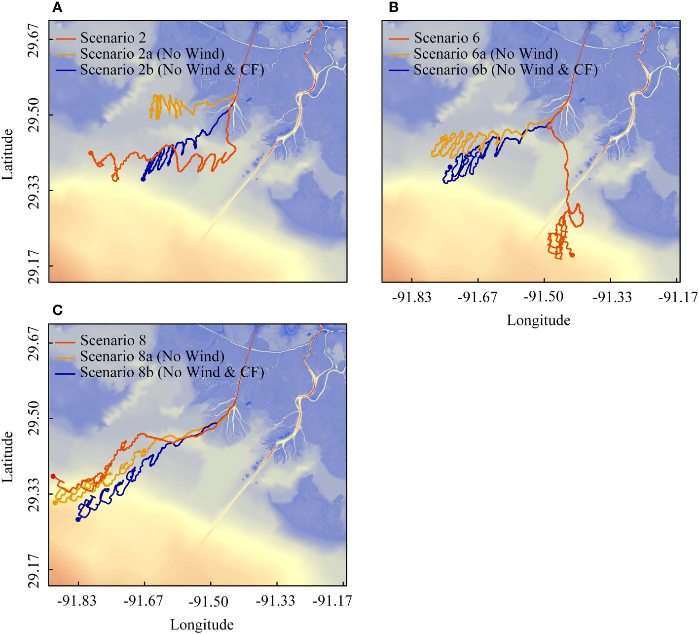
Figure 12 Trajectory of particles using a LAgrangian model for 8 days. (A) Trajectory of particles during Scenarios 2, 2a, and 2b, (B) Trajectory of particles during Scenarios 6, 6a, 6b, (C) Trajectory of particles during Scenarios 8, 8a, and 8b.
The sediment transport process is a key driver to build and maintain the delta’s landmass, with sediment deposited in the delta causing the delta to expand (e.g., Olliver et al., 2020). This expansion provides new habitats for wildlife, as well as providing coastal protection from erosion. The WLD is formed by sediment delivered by the Atchafalaya River, which is then transported and deposited in the WLO. The sediment transport and accretion in the WLD and Atchafalaya Bay can be regulated by water level variation, water volume transport, and water current induced by winter winds (Elsayed and Oumeraci, 2017; HRECOS, 2017; Kemp et al., 2017; Li et al., 2017).
The formation and maintenance of wetlands is a crucial topic in the Wax Lake Delta. Variations in water level and water transport have a profound impact on the wetlands in the WLD, as they can lead to the flooding or draining of wetlands, which affects their productivity and capacity to keep pace with sea level rise (Roberts et al., 2015; Olliver and Edmonds, 2017). Depending on the duration, flooding can negatively impact many beneficial functions of wetlands such as fish and wildlife habitats and nutrient removal and can harm upland plant species (Nyman et al., 2006; Hiatt et al., 2018).
The results of this work indicate that, among the cases we investigated, the westerly cold fronts have the most significant impact on water level variations and volume transport in channels and bays, followed by northwesterly and northerly cold fronts. Using a uniform probability distribution on monitoring data provided by NOAA’s Hydrometeorological Prediction Center (HPC, 2023), we analyzed 631 cold front events that occurred between 2010 and 2022 and determined that the probability of northwesterly cold fronts is the most common, making up 44% of all cold fronts, while northerly and westerly cold fronts account for 32% and 0.24%, respectively. Additionally, the analysis shows that the impacts of cold fronts on water level variation, subtidal current, and transport processes are more pronounced when the WLO discharge is low (less than 2000 m3/s or lower). The probability of a cold front occurring during low discharge conditions is approximately 0.28 based on the uniform distribution analysis for cold fronts between 2010 and 2022.
Despite these analyses, there remains a gap in understanding how cold fronts influence the spatial pattern of sediment transport and concentration in deltaic environments. Future research should address the impacts of cold fronts for sedimentation and erosion in complex deltaic environments and evaluate the importance of such periodic forcings on long-term deltaic sustainability. Such analyses will become more important as restoration activities aiming to leverage deltaic land-building processes, such as sediment diversions in Louisiana (e.g., Allison and Meselhe, 2010), are increasingly used to mitigate coastal hazards and land loss.
This study analyzes how cold fronts influence the hydrodynamics of the Wax Lake Delta (WLD) by considering various forcing factors including the orientation and moving direction of the cold front, Wax Lake Outlet (WLO) discharge, the intensity of the wind, and the Coriolis effect. To examine the hydrodynamics of wind-driven circulations caused by cold fronts, the study utilized two numerical models, Delft3D-FLOW and Delft3D-WAQ PART, to simulate 9 different cold fronts. Apart from the simulations, an analytic model was also employed to analyze the effects of both remote and local forces on water level fluctuations in an idealized bay.
The study confirms that the Gadwall Pass is the most significant channel for water transport, accounting for around 27% of the total, followed by the Greg Pass, which accounts for 18%. The results also found that cold fronts generally cause a decrease in the average contribution of western channels, while there is an increase in the central and eastern channels. Furthermore, the results conclude that the volume of water transported through secondary channels and the intrusion into wetlands decrease during cold fronts, mainly due to the low water depth in the primary channels at this time. In terms of subtidal water level, the maximum variations happen in Canvasback Bay, Fred Island, Tim Island, Mike Island, Greg Island, and East Bay. These changes are primarily caused by local wind stress, and their magnitude depends on factors such as the intensity of wind, cold front’s moving direction, and the WLO discharge rate. For example, a westerly cold front can lead to a water level variation of approximately 0.45 m on Mike and Tim Islands, while East Bay can experience a variation of up to 0.65 m.
The study revealed that the primary pattern of subtidal water circulation in the Wax Lake Delta involves water flowing out from Atchafalaya Bay towards the southwest side. However, this circulation pattern can be altered, and even reversed, by changes in the WLO discharge and the strength of the cold front. In a strong northwesterly cold front, the average subtidal current in the Gadwall Pass and Atchafalaya Bay can reach 1.5 m/s and 0.8 m/s to the southwest, respectively. In contrast to typical conditions, the streamlines in Atchafalaya Bay undergo a northward shift during the pre-frontal passage phase when the discharge rate of WLO is relatively low (less than 2000 m3/s) because the prefrontal southerly wind overcomes the river discharge.
When the outflow momentum dominates over the wind and Coriolis forces, most of the particles exit the Wax Lake delta through the Gadwall Pass and then flow towards the west side of the bay due to the Coriolis force. However, a robust cold front can cause the particles to exit through the Main Pass and flow towards the east side. Additionally, the study found that the Coriolis force plays a crucial role in determining the trajectory of particles exiting from WLO, particularly when the WLO discharge is low.
Overall, the results suggest that the passage of cold fronts can significantly impact the hydrodynamics of the Wax Lake Delta, which can have implications for the transport of sediment and nutrients, wetland productivity, and wildlife habitats. These effects are more pronounced when the discharge of WLO is low and during westerly cold fronts. The study also found that westerly cold fronts have the most significant impact on the hydrodynamics of Atchafalaya Bay, followed by the northwesterly and northerly cold fronts.
The original contributions presented in the study are included in the article/supplementary material. Further inquiries can be directed to the corresponding author.
CL: conceptualization, methodology, supervision, review, and editing. SF: methodology, software, validation, formal analysis, writing original draft. MH: conceptualization, methodology, supervision, review, and editing. All authors contributed to the article and approved the submitted version.
This research was supported by the National Science Foundation (EAR-2023443), and partially supported by the Gulf of Mexico Coastal Ocean Observing Systems and NOAA Cooperative Agreement#NA16NOS0120018.
The authors acknowledge that the opensource datasets used in the study were from NASA, NOAA, USGS, NGDC, etc. (see the text for details). Some of the meteorology data was from WAVCIS. Support from NSF, NOAA, GCOOS, and LSU is greatly appreciated.
The authors declare that the research was conducted in the absence of any commercial or financial relationships that could be construed as a potential conflict of interest.
All claims expressed in this article are solely those of the authors and do not necessarily represent those of their affiliated organizations, or those of the publisher, the editors and the reviewers. Any product that may be evaluated in this article, or claim that may be made by its manufacturer, is not guaranteed or endorsed by the publisher.
Allison M. A., Meselhe E. A. (2010). The use of large water and sediment diversions in the lower Mississippi River (Louisiana) for coastal restoration. J. Hydrol. 387 (3–4), 346–360. doi: 10.1016/j.jhydrol.2010.04.001
Cao Y., Li C., Dong C. (2020). Atmospheric cold front-generated waves in the coastal Louisiana. J. Mar. Sci. Eng. 8 (11), 900. doi: 10.3390/jmse8110900
Castellanos D. L., Rozas L. P. (2001). Nekton use of submerged aquatic vegetation, marsh, and shallow unvegetated bottom in the Atchafalaya River Delta, a Louisiana tidal freshwater ecosystem. Estuaries 24 (2), 184–197. doi: 10.2307/1352943
Chaichitehrani N., Li C., Xu K., Allahdadi M. N., Hestir E. L., Keim B. D., et al. (2019). A numerical study of sediment dynamics over Sandy Point dredge pit, west flank of the Mississippi River, during a cold front event. Continental Shelf Res. 183, 38–50. doi: 10.1016/j.csr.2019.06.009
Childers D. L., Day J. W. (1990). Marsh-water column interactions in two Louisiana estuaries. I. Sediment dynamics. Estuaries 13 (4), 393–403. doi: 10.2307/1351784
Deltares (2018). Delft3D-FLOW user manual, simulation of multi-dimensional hydrodynamic flows and transport phenomena, including sediments. Delft, Netherlands: Deltares.
Denbina M. W., Simard M., Pavelsky T. M., Christensen A. I., Liu K., Lyon C. (2020). Pre-Delta-X: Channel Bathymetry of the Atchafalaya Basin, LA, USA 2016 (Oak Ridge, Tennessee, USA: ORNL Distributed Active Archive Center). doi: 10.3334/ORNLDAAC/1807
Denes T. A., Caffrey J. M. (1988). Changes in seasonal water transport in a Louisiana estuary, Fourleague Bay, Louisiana. Estuaries 11 (3), 184–191. doi: 10.2307/1351971
Elsayed S. M., Oumeraci H. (2017). Effect of beach slope and grain-stabilization on coastal sediment transport: An attempt to overcome the erosion overestimation by XBeach. Coast. Eng. 121 (December 2016), 179–196. doi: 10.1016/j.coastaleng.2016.12.009
Feizabadi S., Rafati Y., Ghodsian M., Akbar Salehi Neyshabouri A., Abdolahpour M., Mazyak A. R. (2022). Potential sea-level rise effects on the hydrodynamics and transport processes in Hudson–Raritan Estuary, NY–NJ. Ocean Dynam. 72 (6), 421–442. doi: 10.1007/s10236-022-01512-0
Feng Z., Li C. (2010). Cold-front-induced flushing of the Louisiana bays. J. Mar. Syst. 82 (4), 252–264. doi: 10.1016/j.jmarsys.2010.05.015
Gallucci F., Netto S. A. (2004). Effects of the passage of cold fronts over acoastal site: an ecosystem approach. Mar. Ecol. Prog. Ser. 281, 79–92. doi: 10.3354/meps281079
Garvine R. W. (1985). A simple model of estuarine subtidal fluctuations forced by local and remote wind stress. J. Geophys. Res.: Oceans 90 (C6), 11945–11948. doi: 10.1029/JC090iC06p11945
Georgiou I. Y., FitzGerald D. M., Stone G. W. (2005). The impact of physical processes along the Louisiana coast. J. Coast. Res. 44, 7289. Available at: http://www.jstor.org/stable/25737050.
Hiatt M., Castañeda‐Moya E., Twilley R., Hodges B. R., Passalacqua P. (2018). Channel-island connectivity affects water exposure time distributions in a coastal river delta. Water Resour. Res. 54 (3), 2212–2232. doi: 10.1002/2017WR021289
Hiatt M., Snedden G., Day J. W., Rohli R. V., Nyman J. A., Lane R., et al. (2019). Drivers and impacts of water level fluctuations in the Mississippi River delta: Implications for delta restoration. Estuarine Coast. Shelf Sci. 224, 117–137. doi: 10.1016/j.ecss.2019.04.020
Hiatt M., Passalacqua P. (2015). Hydrological connectivity in river deltas: The first-order importance of channel-island exchange. Water Resour. Res. 51 (4), 2264–2282. doi: 10.1002/2014WR016149
Hiatt M., Passalacqua P. (2017). What controls the transition from confined to unconfined flow? Analysis of hydraulics in a coastal river delta. J. Hydraulic Eng. 143 (6), 3117003. doi: 10.1061/(ASCE)HY.1943-7900.0001309
Honda K., Terada T., Yoshida Y., Isitani D. (1908). Secondary undulations of oceanic tides. J. Coll. Science Imperial Univ. Tokyo Japan 24, 1113. doi: 10.11429/PTMPS1907.4.4_79
HPC. (2023). NOAA’s Hydrometeorological Prediction Center. Available at: https://www.wpc.ncep.noaa.gov/index.shtmlpage=ovw.
HRECOS. (2017). Hudson River Environmental Conditions Observing System. Available at: https://www.hrecos.org/ (Accessed 25 May 2017).
Huang W., Li C. (2017). Cold front driven flows through multiple inlets of Lake Pontchartrain Estuary. J. Geophys. Res.: Oceans 122 (11), 8627–8645. doi: 10.1002/2017JC012977
Janzen C. D., Wong K. (2002). Wind-forced dynamics at the estuary-shelf interface of a large coastal plain estuary. J. Geophys. Res.: Oceans 107 (C10), 1–2. doi: 10.1029/2001JC000959
Kamphuis J. W. (2020). Introduction to coastal engineering and management. Third edit, advanced series on ocean engineering (Third Edit: World Scientific). doi: 10.1142/7021
Kantha L. (2005). “Barotropic Tides in the Gulf of Mexico. Circulation in the Gulf of Mexico: Observations and Models,” in American Geophysical Union Geophysical Monograph Series, (Wiley Online Library). 161, 159–163. doi: 10.1029/161GM13
Kemp A. C., Hill T. D., Vane C. H., Cahill N., Orton P. M., Talke S. A., et al. (2017). Relative sea-level trends in New York City during the past 1500 years. Holocene 27 (8), 1169–1186. doi: 10.1177/0959683616683263
Kourafalou V. H., Oey L., Wang J. D., Lee T. N. (1996). The fate of river discharge on the continental shelf: 1. Modeling the river plume and the inner shelf coastal current. J. Geophys. Res.: Oceans 101 (C2), 3415–3434. doi: 10.1029/95JC03024
Li C. (2003). Can friction coefficient be estimated from cross stream flow structure in tidal channels? Geophys. Res. Lett. 30 (17), 1897. doi: 10.1029/2003GL018087
Li C. (2013). Subtidal water flux through a multiple-inlet system: Observations before and during a cold front event and numerical experiments. J. Geophys. Res.: Oceans 118 (4), 1877–1892. doi: 10.1002/jgrc.20149
Li C., Roberts H., Stone G. W., Weeks E., Luo Y. (2011). Wind surge and saltwater intrusion in Atchafalaya Bay during onshore winds prior to cold front passage. Hydrobiologia 658 (1), 27–39. doi: 10.1007/s10750-010-0467-5
Li C., Weeks E., Huang W., Milan B., Wu R. (2018). Weather-induced transport through a tidal channel calibrated by an unmanned boat. J. Atmos. Oceanic Technol. 35 (2), 261–279. doi: 10.1175/JTECH-D-17-0130.1
Li C., Huang W., Wu R., Sheremet A. (2020). Weather induced quasi-periodic motions in estuaries and bays: Meteorological tide. China Ocean Eng. 34 (3), 299–313. doi: 10.1007/s13344-020-0028-2
Li C., Huang W., Milan B. (2019). Atmospheric cold front–induced exchange flows through a microtidal multi-Inlet Bay: analysis using multiple horizontal ADCPs and FVCOM simulations. J. Atmos. Oceanic Technol. 36 (3), 443–472. doi: 10.1175/JTECH-D-18-0143.1
Li M., Li C. (2022). Comparison of Flows through a Tidal Inlet in Late Spring and after the Passage of an Atmospheric Cold Front in Winter Using Acoustic Doppler Profilers and Vessel-Based Observations. Sensors 22 (9), 3478. doi: 10.3390/s22093478
Li Y., Li C., Li X. (2017). Remote sensing studies of suspended sediment concentration variations in a coastal bay during the passages of atmospheric cold fronts. IEEE J. Selected Topics Appl. Earth Observ. Remote Sens. 10 (6), 2608–2622. doi: 10.1109/JSTARS.2017.2655421
Li C., O’Donnell J. (1997). Tidally driven residual circulation in shallow estuaries with lateral depth variation. J. Geophys. Res.: Oceans 102 (C13), 27915–27929. doi: 10.1029/97JC02330
Murray S. P. (1975). Trajectories and speeds of wind-driven currents wear the coast. J. Phys. Oceanogr. 5 (2), 347–360. doi: 10.1175/1520-0485(1975)005<0347:TASOWD>2.0.CO;2
NGDC. (2001). U.S. Coastal Relief Model Vol.4 - Central Gulf of Mexico. Available at: https://www.ncei.noaa.gov/products/coastal-relief-model.
NOAA. (2022). Tides and Currents. Available at: https://tidesandcurrents.noaa.gov/.
Nyman J. A., Walters R. J., Delaune R. D., Patrick W. H. Jr. (2006). Marsh vertical accretion via vegetative growth. Estuarine Coast. Shelf Sci. 69 (3–4), 370–380. doi: 10.1016/j.ecss.2006.05.041
Olliver E. A., Edmonds D. A. (2017). Defining the ecogeomorphic succession of land building for freshwater, intertidal wetlands in Wax Lake Delta, Louisiana. Estuarine Coast. Shelf Sci. 196, 45–57. doi: 10.1016/j.ecss.2017.06.009
Olliver E. A., Edmonds D. A. (2021). Hydrological connectivity controls magnitude and distribution of sediment deposition within the deltaic islands of Wax Lake Delta, LA, USA. J. Geophys. Res.: Earth Surface, (Wiley Online Library), 126.
Olliver E. A., Edmonds D. A., Shaw J. B. (2020). Influence of floods, tides, and vegetation on sediment retention in Wax Lake Delta, Louisiana, USA. J. Geophys. Res.: Earth Surface 125 (1), e2019JF005316. doi: 10.1029/2019JF005316
Payandeh A. R., Justic D., Mariotti G., Huang H., Sorourian S. (2019). Subtidal water level and current variability in a bar-built estuary during cold front season: Barataria Bay, Gulf of Mexico. J. Geophys. Res.: Oceans 124 (10), 7226–7246. doi: 10.1029/2019JC015081
Perez B. C., Day J. W. Jr., Rouse L. J., Shaw R. F., Wang M. (2000). Influence of Atchafalaya River discharge and winter frontal passage on suspended sediment concentration and flux in Fourleague Bay, Louisiana. Estuarine Coast. Shelf Sci. 50 (2), 271–290. doi: 10.1006/ecss.1999.0564
Pihl J. H., Bredmose H., Larsen J. (2001). Shoaling of sixth-order Stokes waves on a current. Ocean Eng. 28 (6), 667–687. doi: 10.1016/S0029-8018(00)00017-2
Powell N. (1996). The wax lake outlet weir and channel response. III. Fluvial: Channel Evol. Channel Stabil., 4653.
Pritchard D. W. (1952). Salinity distribution and circulation in the Chesapeake Bay estuarine system. Mar. Res. 11, 106–123.
Roberts H. H., Huh O. K., Hsu S. A., Rouse L. J. Jr., Rickman D. A. (1989). Winter storm impacts on the chenier plain coast of southwestern Louisiana. Gulf Coast Association of Geological Societies Transactions 39, 515522.
Roberts H. H., DeLaune R. D., White J. R., Li C., Sasser C. E., Braud D., et al. (2015). Floods and cold front passages: impacts on coastal marshes in a river diversion setting (Wax Lake Delta Area, Louisiana). J. Coast. Res. 31 (5), 1057–1068. doi: 10.2112/JCOASTRES-D-14-00173.1
Rosen T., Xu Y. J. (2013). Recent decadal growth of the Atchafalaya River Delta complex: Effects of variable riverine sediment input and vegetation succession. Geomorphology 194, 108–120. doi: 10.1016/j.geomorph.2013.04.020
Rubinstein R. Y. (1981). Simulation and the monte carlo method. New York, NY, USA: John Wiley & Sons.
Salas-Monreal D., Valle-Levinson A. (2008). Sea-level slopes and volume fluxes produced by atmospheric forcing in estuaries: Chesapeake Bay case study. J. Coast. Res. 24 (10024), 208–217. doi: 10.2112/06-0632.1
Snedden G. A., Cable J. E., Wiseman W. J. (2007). Subtidal sea level variability in a shallow Mississippi River deltaic estuary, Louisiana. Estuaries Coasts 30 (5), 802–812. doi: 10.1007/BF02841335
Swenson E. M., Chuang W.-S. (1983). Tidal and subtidal water volume exchange in an estuarine system. Estuarine Coast. Shelf Sci. 16 (3), 229–240. doi: 10.1016/0272-7714(83)90142-7
Szpilka C., Dresback K., Kolar R., Massey T. C. (2018). Improvements for the Eastern North Pacific ADCIRC tidal database (ENPAC15). J. Mar. Sci. Eng. 6 (4), 131. doi: 10.3390/jmse6040131
Ufnar D., Ufnar J. A., Ellender R. D., Rebarchik D., Stone G. (2006). Influence of coastal processes on high fecal coliform counts in the Mississippi Sound. J. Coast. Res. 22 (6), 1515–1526. doi: 10.2112/04-0434.1
USGS. (2023). National Water Information System: Web Interface. Available at: http://waterdata.usgs.gov/nwis/measurements/?site_no=07381590.
Van Beek J. L. (1979). 'Hydraulics of the Atchafalaya main channel system, consideration from a multiuse management standpoint' Report No. EPA-600/4-79-036. Las Vegas, NV: Environmental Monitoring and Support Laboratory, Environmental Protection Agency, 36 pp.
Wagner W., Mohrig D. (2019). Flow and sediment flux asymmetry in a branching channel delta. Water Resour. Res. 55 (11), 9563–9577. doi: 10.1029/2019WR026050
Walker N. D., Hammack A. B. (2000). Impacts of winter storms on circulation and sediment transport: Atchafalaya-Vermilion Bay region, Louisiana, USA. J. Coast. Res. 16 (4), 996–1010.
Wang D.-P., Elliott A. J. (1978). Non-tidal variability in the Chesapeake Bay and Potomac River: Evidence for non-local forcing. J. Phys. oceanogr. 8 (2), 225–232. doi: 10.1175/1520-0485(1978)008<0225:NTVITC>2.0.CO;2
Wang J., Li C., Xu F., Huang W. (2020). Severe weather-induced exchange flows through a narrow tidal channel of Calcasieu Lake Estuary. J. Mar. Sci. Eng. 8 (2), 113. doi: 10.3390/jmse8020113
Willmott C. J. (1981). ON THE VALIDATION OF MODELS. Phys. Geogr. 2 (2), 184–194. doi: 10.1080/02723646.1981.10642213
Wilson J. D., Sawford B. L. (1996). Review of Lagrangian stochastic models for trajectories in the turbulent atmosphere. Boundary-layer meteorol. 78, 191–210. doi: 10.1007/BF00122492
Wong K., Garvine R. W. (1984). Observations of wind-induced, subtidal variability in the Delaware Estuary. J. Geophys. Res.: Oceans 89 (C6), 10589–10597. doi: 10.1029/JC089iC06p10589
Wu J. (1980). Wind-stress coefficients over sea surface near neutral conditions—A revisit. J. Phys. Oceanogr. 10 (5), 727–740. doi: 10.1175/1520-0485(1980)010<0727:WSCOSS>2.0.CO;2
Wu J. (1994). The sea surface is aerodynamically rough even under light winds. Boundary-layer meteorol. 69 (1), 149–158. doi: 10.1007/BF00713300
Keywords: Wax Lake Delta, cold front, effect of frontal moving direction, hydrodynamics response, particle tracking, coriolis force, three-dimensional model (3D)
Citation: Feizabadi S, Li C and Hiatt M (2023) A numerical experiment of cold front induced circulation in Wax Lake Delta: evaluation of forcing factors. Front. Mar. Sci. 10:1228446. doi: 10.3389/fmars.2023.1228446
Received: 24 May 2023; Accepted: 11 September 2023;
Published: 29 September 2023.
Edited by:
Xiaohui Xie, Ministry of Natural Resources, ChinaReviewed by:
Jilian Xiong, University of Washington, United StatesCopyright © 2023 Feizabadi, Li and Hiatt. This is an open-access article distributed under the terms of the Creative Commons Attribution License (CC BY). The use, distribution or reproduction in other forums is permitted, provided the original author(s) and the copyright owner(s) are credited and that the original publication in this journal is cited, in accordance with accepted academic practice. No use, distribution or reproduction is permitted which does not comply with these terms.
*Correspondence: Chunyan Li, Y2xpQGxzdS5lZHU=
Disclaimer: All claims expressed in this article are solely those of the authors and do not necessarily represent those of their affiliated organizations, or those of the publisher, the editors and the reviewers. Any product that may be evaluated in this article or claim that may be made by its manufacturer is not guaranteed or endorsed by the publisher.
Research integrity at Frontiers
Learn more about the work of our research integrity team to safeguard the quality of each article we publish.