Methods to get more information from sparse vessel monitoring systems data

Vessel Monitoring Systems (VMS) and other vessel tracking data have been used for many years to map the distribution of fishing activities. Mapping areas with low levels of fishing activity can be of particular interest; for example to avoid conflicts between fishing and other ocean uses like offshore renewable energy or to protect relatively pristine ecosystems from increasing fishing pressure. A particular problem when trying to delineate areas that are lightly fished, is the relative sparsity of vessel monitoring data in these areas. This paper explores three novel methods for estimating the distribution of fishing activity from VMS data, with particular focus on lightly impacted areas. The first new method divides the area of interest into a nested grid with varying cell sizes (depending on the density of data at each location); the second new method uses Voronoi diagrams to define polygons around observations and the third method applies a local regression to generate a smooth map of fishing intensity. The new methods are compared with two established methods: applying spatial grids and interpolating fishing tracks. The track interpolation method generally performs better than any of the new methods, however it is not always possible or appropriate to apply track interpolation; in those cases the local regression method is the best alternative.

1 Introduction

Automated vessel tracking data have been used for many years to map the distribution of fishing activities; for example, 25 years ago the spatial distribution of beam trawl effort in the North Sea was mapped in detail (Rijnsdorp et al., 1998). Since the introduction of satellite-based Vessel Monitoring Systems (VMS) and Automatic Identification Systems (AIS), detailed positional data have been collected for many fishing fleets worldwide. A number of methods have been developed to map the distribution of fishing activities (Lambert et al., 2012) but the most common approach by far is to aggregate the positional data in a spatial grid. These grids may then be used to identify specific fishing grounds (Gerritsen et al., 2012) or quantify the footprint of fishing activity (Gerritsen et al., 2013; Eigaard et al., 2017). Of particular interest is the identification of lightly impacted areas, for example to avoid conflicts between fishing and other ocean uses like offshore renewable energy (Campbell et al., 2014) but also to protect relatively pristine ecosystems from increasing fishing pressure (e.g. ICES, 2022).

A particular problem when trying to map areas that are lightly impacted by fishing is that data will be relatively sparse. For example, the International Council for the Exploration of the Sea (ICES) advises the European Commission on vulnerable marine ecosystems in areas with low fishing pressure by mobile bottom contacting gears (ICES, 2022). ICES uses a threshold of a swept-area ratio (SAR; Gerritsen et al., 2013) of 0.43 to identify areas with low fishing pressure. A SAR of 0.43 means that a given location has a 43% likelihood of being impacted by fishing gear in a year. Bottom trawling impacts an area of roughly 0.6km² per hour of fishing when averaged across gear types and vessel sizes (Eigaard et al., 2016). With a polling interval of 1h, which is common for VMS data, one would therefore expect fewer than one VMS record per km² per year in areas below that threshold. This means that, although VMS datasets typically contain many millions of data points per year, the data are nevertheless sparse in the areas with low fishing activity that we might be interested in.

A well-known problem with the usual approach of gridding VMS data is that the results depend strongly on the resolution used. At a very high resolution (small grid cells), there can be many grid cells with no data points in areas where activity did occur (because VMS data are not a census but a systematic sample of fishing activity). At a low resolution (large grid cells), the spatial detail is lost and the area impacted by fishing is over-estimated because grid cells contain areas of both high and low impact. Rijnsdorp et al. noted this in 1998, but the choice of grid resolution still leads to controversy (Amoroso et al., 2018).

This paper explores existing and new methods of mapping fishing activity from VMS data in areas where data are sparse. All new methods are relatively simple to implement and only require moderate computing power. The performance of these methods is compared with the traditional grid approach and with an established method of interpolating fishing tracks from consecutive positional data points using Hermite splines (Hintzen et al., 2010). In the first ‘new’ method, a grid is constructed with grid cells that vary in size depending on the density of data points by successively splitting large grid cells into smaller ones. This approach removes the choice of a grid resolution and ensures that there are no grid cells without data. It is an adaptation of an approach described by Gerritsen et al. (2013). The second approach is based on constructing tessellating polygons around individual VMS data points by computing a Voronoi diagram (Boots et al., 2009). The surface area of each polygon is then used to calculate the density of fishing activity in each polygon. The third approach applies a local regression and density estimation, using a nearest neighbours approach (Loader, 1999).

2 Methods

2.1 Data

In order to evaluate the methods, an AIS dataset was used; these data are structurally similar to VMS data: they contain a vessel identifier, timestamp, geographic position, speed and heading. However AIS data are available at much shorter time intervals: typically less than 5 minutes versus 1 or 2 hour intervals for VMS data. A major drawback of AIS data is that data are only recorded if they are received by AIS base stations or satellites fitted with AIS receivers. This can result in significant gaps in coverage, particularly in offshore areas. Vessel Monitoring Systems are fully satellite-based and because VMS are mandatory for enforcement purposes, the coverage is close to complete for vessels that are obliged to carry VMS (in Europe this includes all vessels of 12m or more in length). For the current analysis, gaps in the AIS data will not cause problems as the data are only used for exploring the proposed methods and are not intended to provide absolute estimates of the spatial distribution of fishing activity.

As a first step, the AIS data are used to reconstruct actual vessel tracks in order to quantify the ‘true’ fishing footprint (ignoring any inaccuracies in identifying which records correspond to fishing activity as well as missing data). Next, the AIS data are subsampled at time intervals similar to VMS data to test the performance of each method on data that is similar to VMS data.

The AIS data cover the period of one year (2015) and the main case study area is a rectangle of 200km² in size, located in the Irish Sea to the east of Ireland where there was a mix of high and low fishing activity by demersal otter trawlers (see Supplementary Material figure S1 for a map of the case study areas). Approximately 1500 hours of fishing activity took place in the area and 22 vessels were active there. Two additional case study areas were selected to test the methods at different intensities of fishing pressure and using different gears: an area of dredge activity in the eastern Irish Sea and an area of beam trawl activity in the Celtic Sea to the south of Ireland. The dredge case study area was 250km² in size and had around 125 hours of fishing activity by two vessels; the beam trawl case study area was considerably larger: 1200km² with nearly 1000 hours of fishing activity by 7 vessels. The results of these additional case studies are presented in the Supplementary Material (Data Sheet 2).

For the main case study, only fishing vessels that reported using bottom trawls in their logbooks were included. These records were identified by linking the AIS data to the Irish logbooks database using vessel name and activity date. Because the polling frequency of AIS data is variable, the dataset was resampled at intervals close to 5 minutes to create a more consistent dataset. Line segments were created by linking each AIS record to the previous record of the same vessel and the vessel speed was calculated from the length of these lines and the time interval between the records. This calculated speed was assumed to be more representative of the mean vessel speed of the entire segment than the instantaneous speed provided in the AIS dataset. Vessels traveling at speeds between 1.5 and 4.5kn were assumed to be engaged in fishing (following the approach used by Gerritsen and Lordan, 2011) and line segments outside those speed thresholds were removed from the dataset. A buffer was applied to the remaining line segments to approximate the width of the fishing gear (Figure 1). For bottom trawlers the width of the gear was assumed to be 100m (e.g. Gerritsen et al., 2013). The density of fishing activity was then calculated as the time duration represented by each line segment (5 minutes) divided by the surface area of each track segment (100m x the length of the track); at a fishing speed of 6km/h this would work out at 1.67 hours per km². The density values were summed for overlapping track segments and transferred to a fine-scale spatial grid (resolution of 25m x 25m). Finally, a spatial smoother was applied to account for the uncertainty of the actual position of the gear (which is behind and possibly to one side of the vessel position). The smoother uses a moving window filter (focal), calculating a local mean using Gaussian weight function with a 100m standard deviation (Figure 1).

FIGURE 1

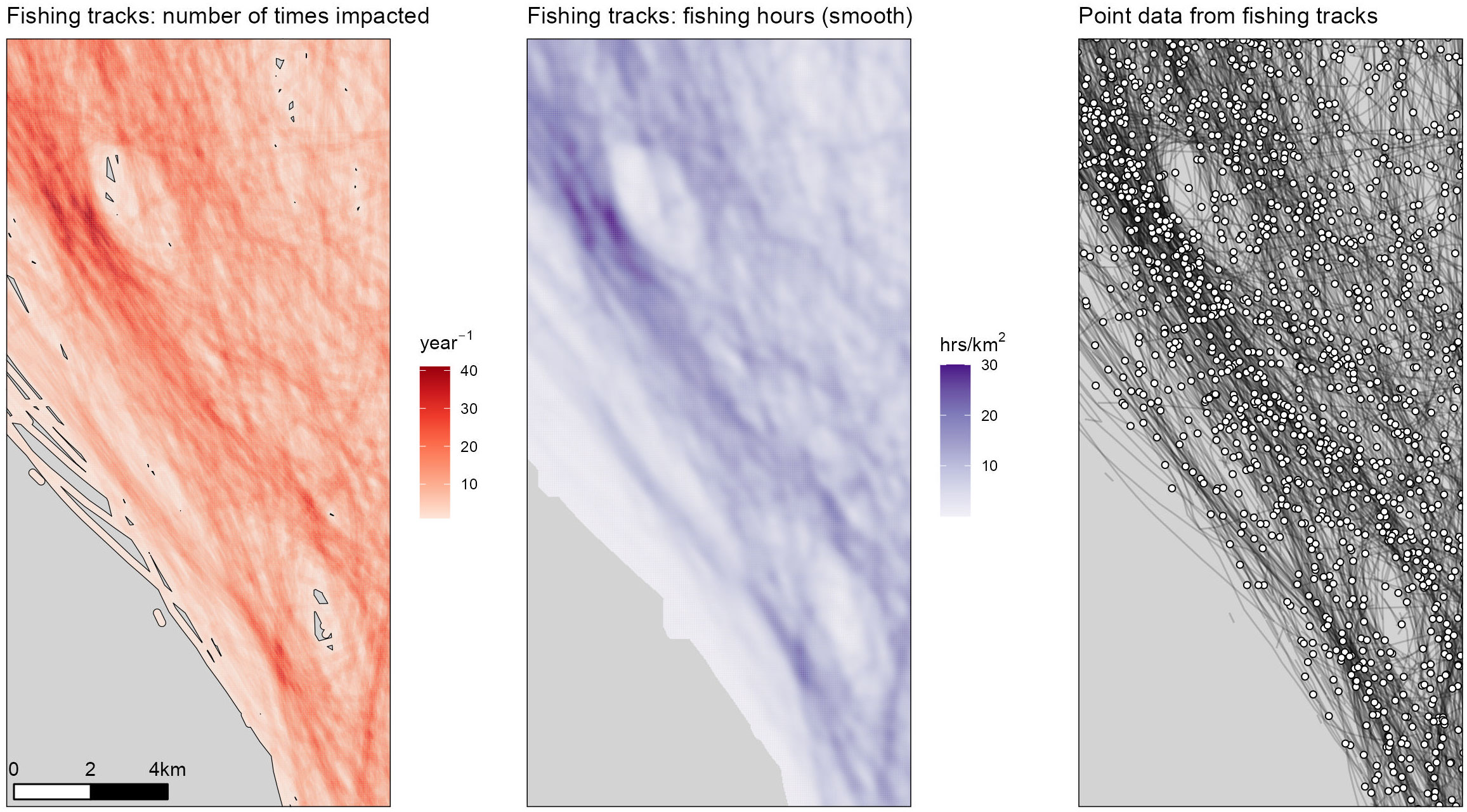
Figure 1 Bottom trawling tracks in the western Irish Sea, obtained from AIS data. Left: tracks with a spatial buffer to account for the width of the fishing gear. The colour scale indicates the number of times each location is impacted by fishing each year. Middle: same data after converting to fishing hours per km² and applying a focal smoother. Right: the points indicate the locations where the AIS data were subsampled at 0.5, 1 or 2h intervals to simulate VMS data.

Recent VMS data from the same region consist of a mix of polling frequencies: around 10% of records are recorded at 20min intervals, 60% at 1h intervals and 30% at 2h intervals. This pattern was mimicked by randomly assigning the 20min, 1h and 2h intervals to vessels in the AIS dataset in the same proportions and subsampling the AIS data at those intervals. Each simulated VMS record was assigned a fishing activity value (hours fished) equal to the interval it was subsampled at so that each record is an unbiased sample of the fishing activity. Both the fishing tracks (AIS) and point data (simulated VMS) were projected using the WGS 84/UTM zone 30N coordinate system.

2.2 Regular grid

The new methods will be compared to the full AIS dataset of ‘true’ fishing tracks but also against established methods, the first one of these is the standard ‘regular grid’ approach. For this purpose, the simulated VMS data are aggregated in spatial grids at three different resolutions: 0.5km x 0.5km; 1km x 1km and 2km x 2km. The level of fishing activity in each grid cell was estimated as the sum of the fishing hours inside each grid cell divided by the surface area of the cell. Figure 2 shows the estimated distribution of fishing activity at those resolutions.

FIGURE 2

Figure 2 Fishing hours per km² estimated by gridding the reduced dataset (which is similar to VMS data) at resolutions of 0.5km x 0.5km (left); 1km x 1km (middle) and 2km x 2km (right).

2.3 Hermite spline interpolation

The second established approach that the new methods will be compared to is the fishing track interpolation described by Hintzen et al. (2010) and implemented in the vmstools R package. The Hermite spline method interpolates the fishing tracks of consecutive data points using vessel speed and heading to define an expected trajectory. The combination of speed and heading are represented by vectors, and vector length is multiplied by a parameter fm that influences the curvature of the interpolations. Before applying the method, the fm parameter first needs to be estimated. This can be done by minimising the distance between actual tracks and interpolated tracks (e.g. https://github.com/nielshintzen/vmstools/wiki/tuneInterpolation). In the current case, the actual tracks are available from the AIS data and the fm parameter was estimated for the main case study area at 0.048 for 20min intervals; 0.091 for 1h intervals and 0.155 for 2h intervals. Figure 3 shows the resulting estimated vessel tracks.

FIGURE 3

Figure 3 Hermite spline track interpolation of the reduced dataset. Left: the point data and interpolated tracks. Middle: tracks converted to fishing hours per km². Right: same data after applying a focal smoother (moving window average).

A drawback of the method is that it can only interpolate between consecutive locations along a fishing track. If a fishing operation is short and only captured by a single VMS record, no interpolation is possible. Similarly, fishing activity will take place for a certain amount of time before the first and after the last VMS position recorded during a fishing operation, leading to additional bias. In the main case study dataset, this led to a loss of 15% of fishing hours. In order to compensate for this bias, the fishing activity estimated from the interpolated tracks was inflated by the commensurate amount: the length of the tracks was unaffected by this but the fishing hours per track segment were increased so the total fishing hours matched those of the input dataset. Finally, a smoother was applied to the distribution of fishing hours (Figure 3), following the same approach outlined for the AIS tracks and for the same reasons.

Other interpolation methods exist, e.g. Russo et al. (2011) used the Catmull–Rom algorithm to refine the spline interpolation approach and Zhao et al. (2020) applied neural networks to deal with trajectories that are not smooth. Both of these methods also address the bias in the Hermite spline approach that is caused by interpolating only between consecutive fishing locations. However, it is not intended to provide a full review of all available methods here and therefore only the most widely cited interpolation approach (Hermite spline) is included in the current analysis.

2.4 Nested grid

The first ‘new’ approach adapts a method described by Gerritsen et al. (2013) which is similar to the simple grid approach but the grid resolution varies in space, depending on the local density of observations. Gerritsen et al. (2013) started with a course rectangular grid and recursively split each grid cell in two equal halves if both halves contained at least n data points, creating a grid of increasingly small rectangles that are nested inside each other. Here, instead of splitting rectangles in equal halves, the rectangles are split to contain equal number of data points by identifying the median x and y position of the points inside the rectangle. Rectangles that are higher than they are wide are split along the x direction rectangles that are wider than high are split along the y direction. A threshold of n=5 was used, meaning that rectangles will not be further split if that would result in fewer than 5 data points in either of the resulting sub-rectangles. Figure 4 illustrates how the approach was applied to the simulated VMS dataset. The datapoints inside each rectangle were aggregated to estimate the total fishing hours in each grid cell and the distribution of fishing activity was estimated by dividing the fishing hours by the surface area of each rectangle.

FIGURE 4

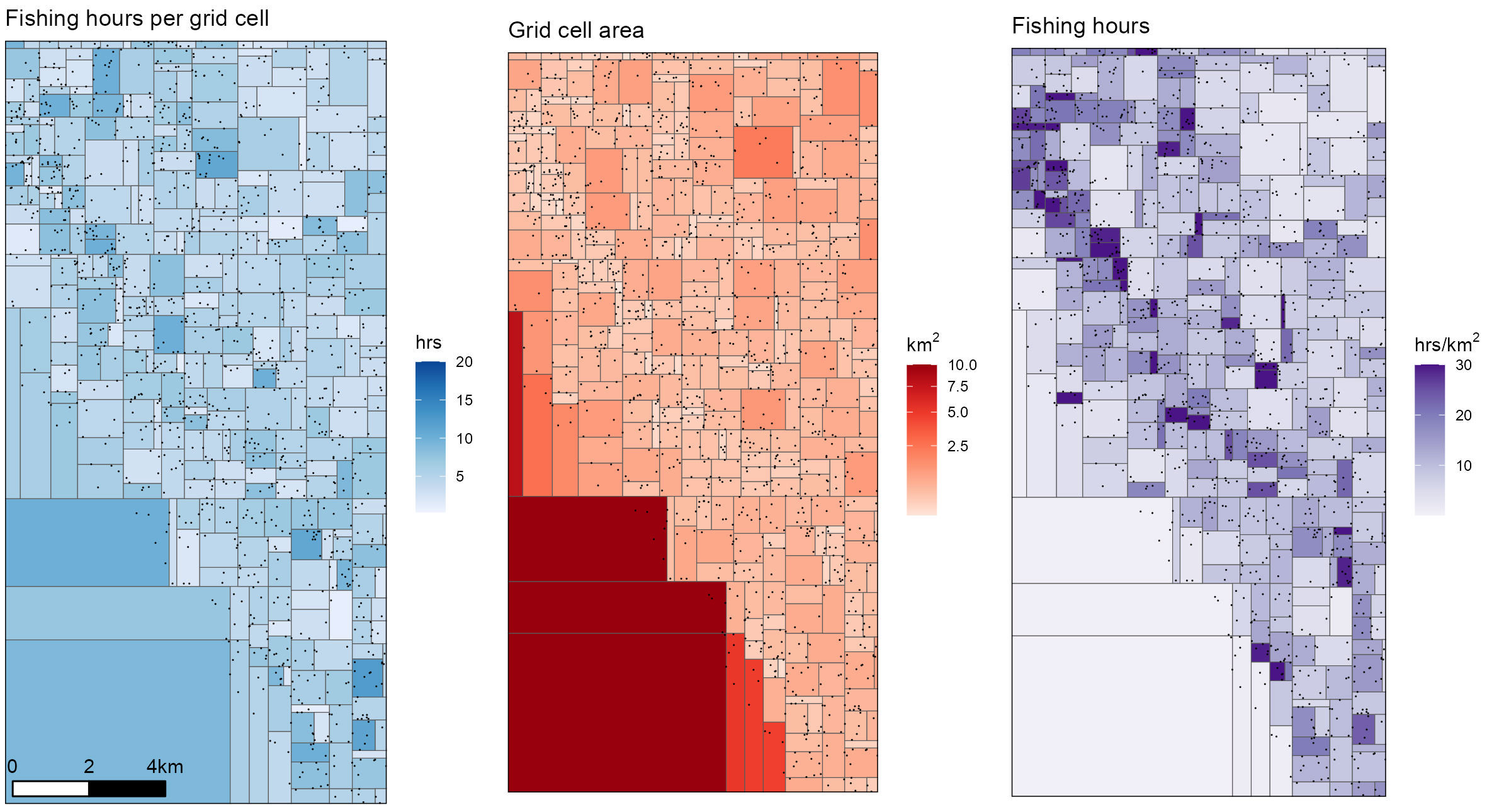
Figure 4 Nested grid approach: grid cells are iteratively split in two until they cannot be further divided without containing at least 5 observations in each cell. This results in a roughly uniform distribution of fishing hours per grid cell (left). This is then divided by the area of each grid cell (middle) to estimate the distribution of fishing hours per km² (right).

2.5 Voronoi

The second new approach is based on creating polygons around individual datapoints – inspired by the way the VAST spatio-temporal model can create maps from prediction grids (Thorson, 2019). However, in areas where these points are very dense, this can generate polygons with very small areas, resulting in noisy density estimates. For this reason, the data were first aggregated at a spatial grid of 100m x 100m. Next a set of tessellating polygons was generated by computing a Voronoi diagram (Boots et al., 2009). Figure 5 illustrates how the approach was applied to the simulated VMS dataset. The fishing hours in each polygon are equal to the fishing hours associated with the relevant data point except in areas of high density where data points were aggregated, resulting in some polygons with fishing hours in excess of 2h. The distribution of fishing activity was estimated by dividing the fishing hours by the surface area of each polygon.

FIGURE 5

Figure 5 Voronoi approach: Voronoi tessellation is applied to the individual observations. To avoid generating very small polygons, the data are first aggregated on a 100m x 100m grid, this results in some polygons that contain data from more than one data point. The fishing hours per polygon are shown on the left. This is then divided by the area of each grid cell (middle) to estimate the distribution of fishing hours per km² (right).

2.6 Local regression

The final new approach deals with two features of the data separately: the response – in this case the hours fished; and the density – the number of data points per km². Due to the nature of the data (where the number of data points is directly proportional to the amount of activity in an area), there is much more information on the spatial structure of the data in areas with high activity than in sparsely exploited areas. This means that any spatial smoothing approach will need to employ a variable bandwidth (otherwise over-smoothing will occur in high-activity areas and under-smoothing in low-activity areas). A local regression and density estimation approach, fitting to a set of nearest-neighbours can deal with this: in high-activity areas the n nearest neighbouring data points will occur within a small area, allowing fine-scale structure to be retained; in low-activity areas, the n nearest neighbours cover a larger area, smoothing out the observations over that larger area.

Loader (1999) describes such a regression and density estimation using local polynomials. This approach is implemented in the locfit R package. The choice of bandwidth has a critical effect on the fit and can be specified as a constant bandwidth or a nearest neighbour bandwidth or a combination of the two. Here, only the nearest neighbour bandwidth is used so that the local neighbourhood always contains a specified number of points. Another important choice is the polynomial degree. A degree of zero is simply a local mean, a degree of one results in a linear regression and higher levels correspond to quadratic and higher degree polynomials. A high-degree polynomial leads to a more variable estimate which may need to be compensated for by increasing the bandwidth. Loader advises that it often suffices to choose a low degree polynomial and focus on choosing the appropriate bandwidth to obtain a satisfactory fit. The final component is the weight function. The (default) tricube weight function was used here; it places less weight on observations that are furthest away and is the traditional weight function for local regression.

A bandwidth based on the n = 20 nearest neighbours was used for both the regression and density estimation – this was based on trial and error and resulted in the least bias and highest precision when compared to the ‘true’ distribution of fishing activity from the AIS dataset. For the regression estimating the distribution of the hours fished per datapoint, a polynomial degree of zero was used; this prevents the model from extrapolating to extreme or negative values in areas with sparse data while the relatively narrow bandwidth makes it flexible enough to account for local differences. For the density estimation a polynomial degree of one was chosen. This allows the model to fit to a local trends in density (which can occur if vessels with a high polling frequency operate in different areas than vessels with a low polling frequency). This is preferable to a traditional kernel density estimate (equivalent to zero degree polynomial), which tends to trim peaks and be biased in the tails.

Figure 6 shows the spatial distributions of predicted mean fishing hours per observation; the density estimate and the fishing hours per km2

FIGURE 6

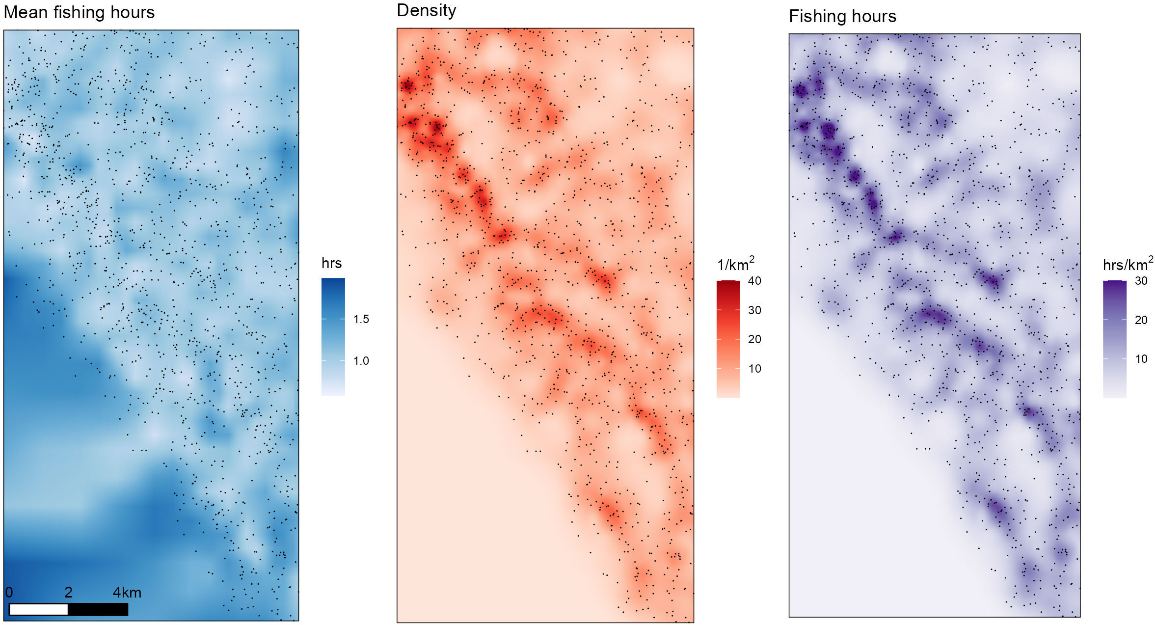
Figure 6 Local fit approach, using the 20 nearest neighbours. The first model estimates mean fishing hours per data point at each location (left); this is expected to be more or less uniformly distributed. The second model estimates the density of observations (middle). The fishing hours per km² are estimated by multiplying the predicted values from the two models (left).

3 Results

The methods described above were used to estimate the part of the case study area that is relatively lightly impacted by fishing, choosing an arbitrary threshold of 5 fishing hours per km² per year in the main case study area. First, the ‘true’ area below the threshold was calculated for the full AIS dataset (Figure 7). The south-western corner of the case study area is not impacted by fishing at all and there are number of smaller areas within the fishing ground which fall below the threshold.

FIGURE 7

Figure 7 The green/blue colour shows the area below the threshold of 5h/km²/year and the orange/brown area is the area above the threshold. The lighter colours refer to areas that were incorrectly assigned, compared to the ’true’ area based on the actual fishing tracks of the full AIS dataset, which is shown in the top-left map. The other maps show the various approaches using the reduced dataset. The spline interpolation approach appears accurately reconstruct the vessel tracks and impacted area from the reduced dataset. The area below the threshold estimated by the regular grid approach depends strongly on the grid resolution (0.5km, 1km and 2km), but at all grid resolutions, there is a relatively large area that is incorrectly classified as being below the threshold; the nested grid approach gives similar results to the 1km grid; the Voronoi approach gives similar results to the 0.5km grid and the local fit approach is reasonably accurate but is too smooth to capture the fine structures that are a few hundred meters in size.

The Hermite spline interpolation appears to be able to accurately reconstruct the fishing tracks from the reduced data set (Figure 7). Visually, this method seems to give the closest approximation of the true area that is below the threshold. This is the only approach that makes use of all available information like speed, heading and the sequence of datapoints of each vessel, making the approach more powerful than the other approaches, which treat each observation as an independent data point.

Figure 7 also shows that the grid-based approaches (unsurprisingly) yield very pixelated results. At the 0.5km grid resolution there are a many grid cells that are incorrectly identified as being below the threshold due to the relative sparsity of the data. The 1km grid resolution appears to give a reasonable estimate of the area below the threshold but the 2km grid resolution is already much too coarse to identify the smaller features that are apparent in the full AIS dataset. The nested grid method settles on a grid size similar to the regular grid of 1km x 1km in areas around the threshold and does not appear to perform any better than the regular grid approach in identifying the outline of the area below the threshold.

The Voronoi approach, like the 0.5km grid, tends to over-estimate the area below the threshold of 5 hours per km². The local fit method comes closest to the true pattern but is unable to recover the same amount of detail as the spline interpolation method (Figure 7).

In order to investigate the performance of the established and new methods at different thresholds, the proportion of the case study area that was incorrectly identified as being below or above each threshold was calculated for a range from 0.5 to 15 hours per km². Figure 8 shows that the spline interpolation method is the most accurate across a the range of thresholds, with generally less than 5% misclassification. At relatively low thresholds, the 0.5km grid over-estimates the area below the threshold. This is because there are too many cells with no data observations. The opposite is true for the 2km grid: the cells are so large that nearly all of them include an area with a relatively large number of data points. The nested grid and Voronoi approaches both tend to over-estimate the area below the threshold for relatively low thresholds. The local fit approach is not as accurate as the spline interpolation but with less than 10% misclassification, it is the second-most accurate method.

FIGURE 8

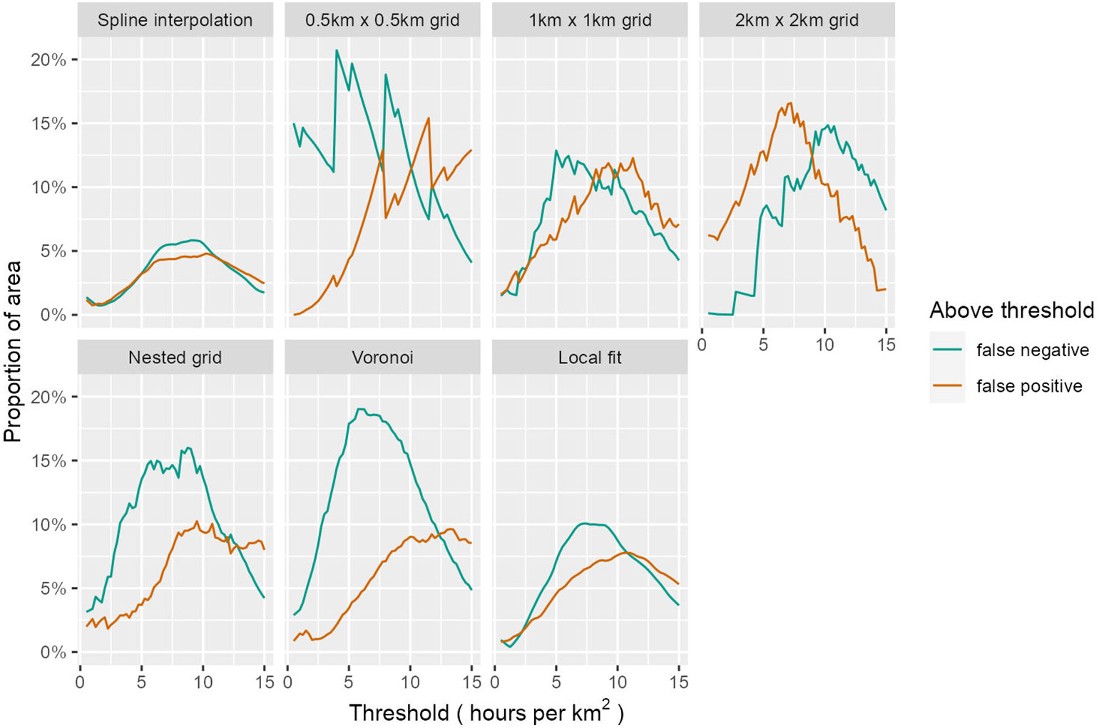
Figure 8 Proportion of the case-study area that was incorrectly classified as being above (false-positive) or below (false negative) various thresholds. The spline interpolation method has highest accuracy at most threshold levels. The fine grid (0.5km) strongly overestimates the area below the threshold up to around 10h/km²/year and the coarse grid (2km) overestimates the area above the threshold up to around 10h/km²/year. The 1km grid seems to be the best compromise of the grid-based approaches for this case study. Both the nested grid and Vonoroi approaches tend to over-estimate the area below the threshold. The local-fit approach does not perform as well as the spline interpolation (although at very low thresholds they are comparable) but it appears to be the most accurate of the point-based methods.

The Supplementary Material (Data Sheet 2) shows the results of the two other case studies. In the case of dredge activity (Figure S2), the Hermite spline method gave visually similar results to the actual fishing tracks (Figures S3, S4) despite the relatively short tracks and sharp turns that are typical in this fishery. In terms of accuracy, the local fit approach performed equally well to the spline interpolation (Figure S5). The beam trawl case study (Figure S6) showed that the Hermite spline method performed best at reconstructing the distribution of fishing activity from the reduced dataset (Figure S7). The local fit and Voronoi methods were both able to identify the main areas of fishing but not individual tracks (Figure S8). In terms of accuracy at different thresholds, the spline interpolation method performed best, followed by the local fit approach (Figure S9).

4 Discussion

The Hermite spline interpolation is the most accurate method of mapping the distribution of fishing activity as well as estimating the area that is below a certain threshold of fishing activity for the case studies examined here. However, interpolation methods are not widely applied in practice. This may be partially due to computational demands of these approaches, which makes it difficult to apply on a large scale. Also, interpolation methods tend to perform poorly when the duration of fishing operations is short, compared to the polling frequency of the data or when the position of the fishing gear is difficult to estimate directly from the vessel position, as is the case in seine and pair-trawl fisheries. In those cases, alternatives need to be considered.

Grid-based methods are by far the most widely used approach to map fishing intensity. These methods are simple to implement and require only moderate computing power. However the choice of the size of the grid cells is highly influential and there is no one-size-fits-all solution. The nested grid approach is intended to address the arbitrary choice of the size of the grid cells with smaller cells in areas of high densities of datapoints. This allows detailed mapping of fine-scale structures in areas with high fishing intensity but for the present purpose (identifying areas with low fishing intensity), the grid cells are necessarily coarse and this method does not perform much better than the a regular grid approach.

The Voronoi method performs reasonably well but is slightly biased in areas where there is a decreasing density of datapoints because it will extend some of the vertices out into untrawled areas: this can be seen in the bottom-left corner of the maps e.g. (Figure 5). The same bias occurs in the nested grid and 2km grid approaches. Like the grid-based approaches, the Voronoi approach is unable to produce smooth surfaces, which could be considered a drawback.

The local fit method is relatively easy to implement on vessel tracking data: it has a well-documented statistical basis (Loader, 1999) and accompanying R package (locfit). It also requires significantly less computing power than track interpolation methods. Because this method does not attempt to reconstruct the fishing tracks, it can be applied to fisheries for which interpolation methods do not work. Another advantage is the fact that the local fit approach estimates the density separately from the response. In the current case study, the response is the amount of fishing activity but any response variable can be modeled: other measures of fishing effort like kW hours; the catch of a certain species; the monetary value of the total catch; etc. The local regression model can then be adapted to the properties of the response variable.

Conclusion: Grid-based methods are widely used but have a number of drawbacks. The Hermite spline interpolation is generally the most accurate approach but track interpolation methods may be difficult to implement on large datasets or in cases where the duration of the fishing operations is relatively short. The local fit approach provides a good alternative in those cases.

Data availability statement

The AIS data analysed in this study were obtained for internal use only from the Irish Coast Guard and cannot be published by the Marine Institute. The Supplementary Material (Data Sheet 1) includes a script to simulate a dataset that can be used to illustrate the approaches described in the article. Historic AIS data are available for a fee from various providers including https://www.marinetraffic.com.

Author contributions

The author confirms being the sole contributor of this work and has approved it for publication.

Acknowledgments

Many thanks to the editor, two reviewers and Guillermo Martin and Cóilín Minto for their valuable feedback.

Conflict of interest

The author declares that the research was conducted in the absence of any commercial or financial relationships that could be construed as a potential conflict of interest.

Publisher’s note

All claims expressed in this article are solely those of the authors and do not necessarily represent those of their affiliated organizations, or those of the publisher, the editors and the reviewers. Any product that may be evaluated in this article, or claim that may be made by its manufacturer, is not guaranteed or endorsed by the publisher.

Supplementary material

The Supplementary Material for this article can be found online at: https://www.frontiersin.org/articles/10.3389/fmars.2023.1223134/full#supplementary-material

References

Amoroso R. O., Parma A. M., Pitcher C. R., McConnaughey R., Jennings S. (2018). Comment on “tracking the global footprint of fisheries”. Science 361, eaat6713. doi: 10.1126/science.aat6713

PubMed Abstract | CrossRef Full Text | Google Scholar

Boots B., Sugihara K., Chiu S. N., Okabe A. (2009). Spatial tessellations: concepts and applications of voronoi diagrams. (Chichester: Wiley & sons, Ltd).

Google Scholar

Campbell M. S., Stehfest K. M., Votier S. C., Hall-Spencer J. M. (2014). Mapping fisheries for marine spatial planning: Gear-specific vessel monitoring system (vms), marine conservation and offshore renewable energy. Mar. Policy 45, 293–300. doi: 10.1016/j.marpol.2013.09.015

CrossRef Full Text | Google Scholar

Eigaard O. R., Bastardie F., Breen M., Dinesen G. E., Hintzen N. T., Laffargue P., et al. (2016). Estimating seabed pressure from demersal trawls, seines, and dredges based on gear design and dimensions. ICES. J. Mar. Sci. 73, i27–i43. doi: 10.1093/icesjms/fsw116

CrossRef Full Text | Google Scholar

Eigaard O. R., Bastardie F., Hintzen N. T., Buhl-Mortensen L., Buhl-Mortensen P., Catarino R., et al. (2017). The footprint of bottom trawling in european waters: distribution, intensity, and seabed integrity. ICES. J. Mar. Sci. 74, 847–865. doi: 10.1093/icesjms/fsw194

CrossRef Full Text | Google Scholar

Gerritsen H., Lordan C. (2011). Integrating vessel monitoring systems (vms) data with daily catch data from logbooks to explore the spatial distribution of catch and effort at high resolution. ICES. J. Mar. Sci. 68, 245–252. doi: 10.1093/icesjms/fsq137

CrossRef Full Text | Google Scholar

Gerritsen H., Lordan C., Minto C., Kraak S. (2012). Spatial patterns in the retained catch composition of irish demersal otter trawlers: High-resolution fisheries data as a management tool. Fisheries. Res. 129, 127–136. doi: 10.1016/j.fishres.2012.06.019

CrossRef Full Text | Google Scholar

Gerritsen H. D., Minto C., Lordan C. (2013). How much of the seabed is impacted by mobile fishing gear? absolute estimates from vessel monitoring system (vms) point data. ICES. J. Mar. Sci. 70, 523–531. doi: 10.1093/icesjms/fst017

CrossRef Full Text | Google Scholar

Hintzen N. T., Piet G. J., Brunel T. (2010). Improved estimation of trawling tracks using cubic hermite spline interpolation of position registration data. Fisheries. Res. 101, 108–115. doi: 10.1016/j.fishres.2009.09.014

CrossRef Full Text | Google Scholar

ICES. (2022). Benchmark Workshop on the occurrence and protection of VMEs (vulnerable marine ecosystems)? (WKVMEBM). Tech. Rep. 4 (44), 98. doi: 10.17895/ICES.PUB.20101637

CrossRef Full Text | Google Scholar

Lambert G. I., Jennings S., Hiddink J. G., Hintzen N. T., Hinz H., Kaiser M. J., et al. (2012). Implications of using alternative methods of vessel monitoring system (vms) data analysis to describe fishing activities and impacts. ICES. J. Mar. Sci. 69, 682–693. doi: 10.1093/icesjms/fss018

CrossRef Full Text | Google Scholar

Loader C. (1999). “Fitting with locfit,” in Local regression and likelihood. (New York: Springer), 45–58.

Google Scholar

Rijnsdorp A., Buys A., Storbeck F., Visser E. (1998). Micro-scale distribution of beam trawl effort in the southern north sea between 1993 and 1996 in relation to the trawling frequency of the sea bed and the impact on benthic organisms. ICES. J. Mar. Sci. 55, 403–419. doi: 10.1006/jmsc.1997.0326

CrossRef Full Text | Google Scholar

Russo T., Parisi A., Cataudella S. (2011). New insights in interpolating fishing tracks from vms data for different metiers.´. Fisheries. Res. 108, 184–194. doi: 10.1016/j.fishres.2010.12.020

CrossRef Full Text | Google Scholar

Thorson J. T. (2019). Guidance for decisions using the vector autoregressive spatio-temporal (vast) package in stock, ecosystem, habitat and climate assessments. Fisheries. Res. 210, 143–161. doi: 10.1016/j.fishres.2018.10.013

CrossRef Full Text | Google Scholar

Zhao Z., Tian Y., Hong F., Huang H., Zhou S. (2020). “Trawler fishing track interpolation using lstm for satellite-based vms traces,” in Global oceans 2020: Singapore–US gulf coast. (New York: IEEE), 1–4.

Google Scholar