Distribution and structure of deep-sea demersal fish assemblages across the central and western Pacific Ocean using data from undersea imagery

Demersal deep-sea fish assemblages from islands and seamounts are poorly described, even in the Hawaiian archipelago. Knowledge across all depths, in similar settings, is even sparser for other archipelagos in the central and western Pacific. However, recent remotely operated vehicle (ROV) explorations and archived video from human-occupied submersible dives conducted by the Hawai`i Undersea Research Laboratory (HURL) provide an opportunity to explore the structure of these assemblages. Here we describe demersal fish assemblages across the central and western Pacific, including in four Marine National Monuments, and examine the relationship of the assemblages to depth and environmental conditions. We used data collected from 227 underwater vehicle dives resulting in the identification of 24,837 individuals belonging to 89 families and 175 genera. The most frequently occurring genera at depths of 250-500 m were Epigonus, Setarches, Polymixia, and Antigonia, between 500-1000 m were Chlorophthalmus, Aldrovandia, and Neocyttus, and between 1000-3000 m were Synaphobranchus, Kumba, Halosaurus, Ilyophis, and Ipnops. There are strong changes in the fish assemblages with depth and region, and assemblages become more similar between regions with greater depth. Depth and region explained the most variance in assemblage structure followed by seafloor particulate organic carbon flux (a food supply proxy), concentrations of dissolved oxygen, and salinity. The Line Islands and Tokelau Ridge had the highest values of seafloor particulate organic carbon flux for all depth zones investigated (250-3000 m) and the highest abundance of fishes at 250-500 m and 500-1000 m, respectively. Taxon accumulation curves indicated that diversity at the genus level within all regions and depth bins (except 1000-2000 m and 2000-3000 m) had not been reached with the existing sampling effort. However, when combining samples from all regions, diversity generally appeared to decrease with depth. Overall, this study demonstrates that there are significant regional differences in the composition of the deep-sea fish fauna as well as differences across depth. Such distribution patterns suggest that the four Marine National Monuments (Papahānaumokuākea, Marianas Trench, Pacific Remote Islands, and Rose Atoll Marine National Monuments, encompassing an area of 3,063,223 km²) are not replicates of diversity, but complementary components of the regional fauna.

1 Introduction

Demersal fish of economic importance are concentrated on the continental shelf and slope to about 1500 m depths (Khedkar et al., 2003; Pitcher et al., 2008), although fisheries for a few deep-sea demersal species also occur on seamounts, guyots, and similar features (Clark et al., 2010). World catches of demersal species increased rapidly during the 20^th century and the limits of biological production have been reached in many areas (Khedkar et al., 2003). Therefore, with the potential for changes in surface primary production induced by climate change to alter standing stocks in the food-limited deep-sea (Glover and Smith, 2003; Smith et al., 2008; Brito-Morales et al., 2020), it is important to understand demersal fish assemblage structure as a key characteristic of these ecosystems.

There have been efforts across the globe to characterize demersal fish assemblage structure, and these have been mostly concentrated on continental shelves and upper slopes, with fewer studies off oceanic islands or on seamounts (Clark et al., 2010; Drazen et al., 2021). The focus has been in the southwestern and southeastern Pacific Ocean (e.g., Koslow et al., 1994; Francis et al., 2002; Tracey et al., 2004), off Japan (e.g., Fujita et al., 1995), the Nazca and Sala-y Gomez Ridges (Parin, 1991; Parin et al., 1997; Tapia-Guerra et al., 2021), across the central Pacific Ocean (Drazen et al., 2021), and in several areas of the North Atlantic (Colvocoresses and Musick, 1984; Haedrich and Merrett, 1990; Mahon et al., 1998; Menezes et al., 2006; Bergstad et al., 2008; Menezes et al., 2009; Morato et al., 2009; Amorim et al., 2017; Parra et al., 2017). These studies have found that depth is a strong driver of assemblage structure with major shifts in fauna between the continental shelf (0-200 m), upper slope (200-600 m), mid-slope (600-800 m), and deep mid-slope (800-1200 m). These studies also found that upper bathyal species exhibited more narrow geographic distributions while deeper species were distributed over broader areas.

Gilbert (1905) and Struhsaker (1973) were the first investigators to focus on demersal fishes in the central Pacific region using trawls to sample species in the Main Hawaiian Islands. Chave and Mundy (1994) synthesized a decade of submersible observations on more than 250 demersal fish taxa between depths of 40 and 2000 meters in both the Main Hawaiian Islands and Northwestern Hawaiian Islands, Johnston Atoll, and Cross Seamount from 1982 to 1992. More recent studies have taken place in the Main Hawaiian Islands (Yeh and Drazen, 2009; De Leo et al., 2012; Oyafuso et al., 2017) and on seamounts in the NWHI (Mejía-Mercado et al., 2019). These studies and those from other regions document changes in assemblage structure with depth. Environmental factors that could be driving these differences, while correlated with depth, are changes in water mass properties (i.e., salinity, temperature, and density), substrate type, food, and oxygen availability (e.g., Labropoulou and Papaconstantinou, 2000). Many of these factors covary with depth. Thus, generalizing how these environmental gradients are correlated with the variation in the distribution and assemblage structure of deep-sea fishes could be greatly expanded by surveying large spatial scales and depth gradients in different regions with variable environmental characteristics.

A recent expansion in ROV exploration throughout the central and western Pacific now provides a means to evaluate demersal fish assemblage structure at a broad scale. NOAA’s CAPSTONE: Campaign to Address Pacific monument Science, Technology, and Ocean NEeds used the NOAA Ship Okeanos Explorer and Deep Discoverer ROV to conduct dives between 2015 and 2017 from the Marianas to American Samoa (Kennedy et al., 2019) and produced a unique data set of deep-sea fishes identified from underwater imagery. Other expeditions using EV Nautilus and ROV Hercules between 2018 and 2019, as well as DSV Pisces IV and V submersible surveys by the Hawai`i Undersea Research Laboratory (HURL) in 2005-2013, augmented the CAPSTONE data and filled geographic gaps in coverage. All dives and their respective imagery platforms will be noted as EV Nautilus, HURL and CAPSTONE hereafter. These datasets provided an opportunity to explore the relationships between fish assemblages and associated geographies and environmental conditions.

In this study, data from undersea imagery were used to survey demersal fish assemblages across varying oceanographic characteristics in the central and western Pacific. Our objectives were to: 1) determine whether the composition, total abundance, and diversity of demersal fish genera differs between regions, and 2) examine what abiotic factors including temperature, depth, salinity, oxygen, and POC flux explain fish distributions and assemblages. All these factors have been postulated to cause faunal zonation with depth (e.g., Labropoulou and Papaconstantinou, 2000) which also may be related to deep-sea water masses and their specific values of temperature, dissolved oxygen, salinity, and density (Richards et al., 1993; Grothues and Cowen, 1999; Galarza et al., 2009). Water masses have been shown to influence the physiology and distribution of organisms in the water column, however studies on deep-sea fishes have found some variables to have a stronger influence than others (Koslow et al., 1994; Yeh and Drazen, 2009).

2 Methods

2.1 Underwater vehicle surveys

Opportunistic data were acquired from underwater vehicle surveys carried out during cruises from multiple expeditions in the central and western Pacific. We used data from NOAA’s three-year Pacific-wide field campaign CAPSTONE that investigated the biodiversity of deep-sea taxa across depths in American Samoa, Johnston Atoll, Line Islands, Main Hawaiian Islands, Musicians Seamounts, Northern Marianas, Northwestern Hawaiian Islands, Southern Marianas, Tokelau Ridge, and Wake Island between July 2015 and September of 2017 (168 dives, 891.5 hours, 0-6000 m depth) (Kennedy et al., 2019).

In addition to the CAPSTONE dives, data from four EV Nautilus cruises (NA101, NA110, NA112, and NA114) between 2018 and 2019 were used from multiple areas within the central and western Pacific (36 dives, ~218 hours, 0- 2459 m) (Kelley et al., 2019), and from submersible dives conducted by HURL between 2005 and 2013 in the Main and Northwestern Hawaiian Islands (the Papahānaumokuākea Marine National Monument) (96 dives,~576 hours, 0-2000 m depth), to fill gaps in geographic extent.

Nearly all data from HURL were collected after 2007 when the use of Ultra-short Baseline (USBL) acoustic positioning systems were implemented to increase tracking and positional accuracy of the underwater vehicles. HURL submersibles used a Tracklink 500HA USBL (LinkQuest) system to calculate the position every 10 seconds (Putts et al., 2019). The US Line Islands and Phoenix Island surveys in 2005 used a Sonardyne USBL system. Both had a horizontal tracking accuracy of approximately 30 m at 1000 m depth. The EV Nautilus and CAPSTONE ROVs also used USBL navigation and calculated position at ≥1 per second (Quattrini et al., 2017). Data from HURL dives include those conducted for quantitative transects as well as opportunistic transits. The tracking data were unavailable for five of these dives, therefore they were not included in the abundance analysis because dive lengths along the seafloor could not be calculated. The full list of dives used in the analysis is available in Supplementary Table 2. Due to the nature of ocean exploration, the dives from any of the vehicles were occasionally interrupted by stopping the ROV or submersible for sampling or for frequent adjustments of the wide-angle view on the forward-facing, high-definition cameras to zoom in on animals for identification and record other ecological attributes (Quattrini et al., 2017). Putts et al. (2019) found that the fields of view of these different camera systems were comparable. Quattrini et al. (2017) combined dives from similar ocean exploration expeditions to investigate demersal fish in the Caribbean; therefore, it was assumed that all vehicles were comparable in their ability to survey fish. All dives, regardless of vehicle, were annotated by the University of Hawai`i Deep-sea Animal Research Center (DARC), using Video Annotation and Reference System (VARS) annotation software.

All vehicles collected temperature, dissolved oxygen, and salinity data from Seabird CTDs. For every observation, the date, geographic position, depth, temperature, salinity, and dissolved oxygen concentration were recorded. There were 227 dives between 2005 and 2019 included in the analysis and they occurred on a variety of rugged features, predominantly rocky seafloor, but including seamounts, atolls, banks, and islands. Since many of the exploration expeditions focused on exploring high-density deep-sea coral and sponge assemblages around seamounts and islands, much of the data acquired are from hard bottom habitats and the authors note that this limits the interpretation of the results, although such bias is systematic throughout the data set.

2.2 Demersal fish data

Taxa were identified to the lowest taxonomic resolution possible, which ranged from class to species. Identifications were made using a variety of taxonomic keys (Compagno, 1984a; Compagno, 1984b; Böhlke, 1989; Cohen et al., 1990; Nakamura and Parin, 1993; Carpenter and Niem, 1999a; Carpenter and Niem, 1999b; Nielsen et al., 1999; Carpenter and Niem, 2001a; Carpenter and Niem, 2001b) and reference images were sent to taxonomic experts for verification. Due to the challenges of identification, many taxa were not identified to species level. Therefore, analyses were performed on data with identification to family and genus level. This was the highest taxonomic resolution that could provide an adequate number of fishes per sample for assemblage structure patterns to emerge. Midwater taxa were removed, which included all Alepocephalidae, Barbourisiidae, Cetomimidae, Chiasmodontidae, Eurypharyngidae, Gonostomatidae, Myctophidae, Nemichthyidae, Phosichthyidae, Scombridae, Sternoptychidae, Stomiidae, Trichiuridae and the zoarcid, Melanostigma spp. Pelagic species were identified based on authors’ experience or by reference to the scientific literature (e.g., Mundy, 2005).

The dives spanned ten different regions (Figure 1) and were split into five depth bins for statistical analysis: 250-500 m, 500-750 m, 750-1000 m, 1000-2000 m, and 2000-3000 m (Table 1). The depth bins were chosen to provide higher resolution (250 m) in upper bathyal water (where assemblage change is more rapid) and lower resolution for depths below 1000 m (Carney, 2005; Zintzen et al., 2017). This depth resolution also corresponded with the analysis by Kennedy et al. (2019) for invertebrate fauna from the CAPSTONE program. The full range of data includes deep-sea fishes between depths of 100 and 5877 m; however, there were not enough observations above 250 m or below 3000 m for a robust analysis, so these observations were omitted. After filtering the data using the above criteria, the number of dives available were 138 from CAPSTONE, 33 from EV Nautilus, and 56 from the HURL records.

FIGURE 1

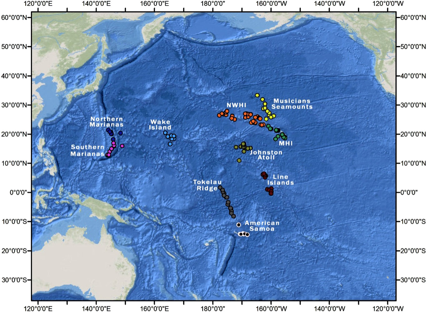
Figure 1 Locations of the 241 samples in the ten regions: AS, American Samoa; JA, Johnston Atoll; MHI, Main Hawaiian Islands; MS, Musicians Seamounts; NM, Northern Marianas; NWHI, Northwestern Hawaiian Islands, the Papahānaumokuākea Marine National Monument; SM, Southern Marianas; WI, Wake Island; LI, Line Islands; TR, Tokelau Ridge in the central and western Pacific. Modified from GEBCO Compilation Group (2023).

TABLE 1

Table 1 The number of samples (dive by depth) with fish observations.

Counts of fishes in depth bins from individual dives will be referred to as samples throughout (Table 1). Samples with five or less fishes observed were removed for the assemblage structure analyses because there are inherently fewer similarities for samples with few individuals. This threshold was chosen based on iterative non-metric Multidimensional Scaling (NMDS) and cluster analysis in which removing samples with five or less fishes produced the least number of outliers. The number of resulting samples at the genus level (n = 212 samples from 151 dives) and family level (n = 241 from 176 dives) varied between regions (refer to Supplementary Data for genus and family level sample data) ranging from 9 to 52 at the family level. In some cases, no samples were available for a depth bin and region because no dives were conducted there, or no samples were possible due to local bathymetry. For example, summits of the Musicians Seamounts reach no shallower than ~1000 m (Cantwell, 2020).

More data were available at the family level, so these were used to investigate trends in abundance, while genus level data we used to investigate assemblage structure. The length of each ROV dive track was used to standardize abundance (fish/m) for each sample. Track length distances varied from 85 m to 7.1 km (Table S1). Dive track distances were measured in ArcMap 10.8.2, consistent with the methods in Kennedy et al. (2019).

2.3 Environmental covariates

There were 24 HURL dives in the Main Hawaiian Islands that did not have salinity or temperature data, and 15 HURL dives in the Northwest Hawaiian Islands that did not have dissolved oxygen data. Therefore, CTD data from dives nearby (within ~50 km) were used to interpolate missing values for the dives that did not have them (Supplementary Table 3).

We used estimates of particulate organic carbon (POC) flux to the seafloor, following methods in Lutz et al. (2007), as a proxy for food supply. Net-Primary-Production (NPP) data were obtained from the Oregon State Ocean Productivity website (http://orca.science.oregonstate.edu/1080.by.2160.monthly.hdf.vgpm.v.chl.v.sst.php), which provided NPP based on the Vertically Generalized Production Model (VGPM). Monthly estimates of NPP data were averaged between 2007 and 2017 at a resolution of 1/6^th of a degree. A fixed euphotic zone depth of 100 m (commonly used as noted in Palevsky and Doney, 2018) was used to calculate Lutz POC flux at the depth for each sample (mid-depth of each sample bin).

Temperature (°C), salinity, and depth (m) were used to identify the water mass encountered by each ROV dive sample (Table 2; Figure 2). Kawabe and Fujio (2010) and Emery (2001) were used to identify water masses in the upper waters (0-500 m), intermediate waters (500-1500 m), and deep waters (≥1500 m). Results of the water mass analyses are included in the Supplementary Material.

TABLE 2

Table 2 Most frequently observed taxa (genus level) between region and depth bin (m).

FIGURE 2

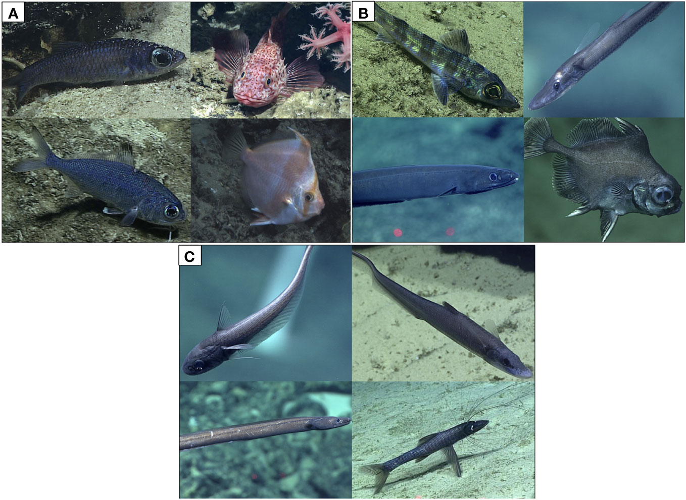
Figure 2 The most frequently observed taxa between depth and region. (A) Most common genera between 250-500 m. Top to bottom and left to right, Epigonus, Setarches, Polymixia, and Antigonia. (B) Most common genera between 500-1000 m, Chlorophthalmus, Aldrovandia, Synaphobranchus, and Neocyttus. (C) Most common genera between 1000 and 3000 m, Kumba, Halosaurus, Ilyophis and Bathypterois. Depth bins combined due to lack of space for photograph panels. See Table 2 for complete lists of frequently observed fishes by region and depth bin. Images courtesy of the NOAA Office of Ocean Exploration and Research.

2.4 Data analysis

Differences in demersal fish assemblage structure between regions and depths were evaluated using PERMANOVA in PRIMER v7 (Clarke and Gorley, 2006) and the program R (Borcard et al., 2011). Assemblage data were visualized using non-metric Multidimensional Scaling (NMDS) ordinations and unconstrained hierarchical clustering. A Mantel test was used to test if differences in assemblage structure between samples covary with the geographic distance between samples. Samples were partitioned into upper bathyal, (250-500 m) intermediate (500-750, 750-1000 m), and deep depths (1000-2000, 2000-3000 m). Genera contributing most to similarity between regions were examined using the Similarity Percentage (SIMPER) analysis with a 70% cutoff for low contributions (Clarke and Gorley, 2006).

We calculated similarities in fish assemblages between all samples using a Bray Curtis similarity matrix. A square-root transformation was used to normalize the variance. As rare genera are expected to be over-represented on geographic features with many samples compared to those with fewer, a Wisconsin double standardization was used to make genera of different abundance equally important (Gauch et al., 1977).

The relationship between assemblage structure and environmental variables was investigated using Canonical Analysis of Principal Coordinates (CAP), a constrained distance-based ordination method, which uses an a priori hypothesis to relate a matrix of response variables, Y (genera) with predictor variables, X (quantitative environmental variables). CAP has the advantage of allowing any distance or dissimilarity measure (e.g., Bray-Curtis) to be used. The CAP was performed on the assemblage data using the function capscale in the R package vegan (Oksanen et al., 2016) and the significance of each environmental variable was determined.

To understand how the abundance of fish varies between regions, we used a General Additive Model (GAM) to investigate the response of total fish abundance recorded in each sample (dive by depth bin) to different environmental variables fit with the “mgcv” package (Hastie and Tibshirani, 2023) in R. Average depth, dissolved oxygen, and salinity were calculated for each sample and used as predictors. The GAM used a negative binomial error distribution with a log link function, and the length of the dive track within the depth bin was included as an offset to account for variation in sampling effort across samples. The “deviance explained” is analogous to variance in a linear regression. The effective degrees of freedom (edf), an approximation of how many parameters the smoother (a parameter that controls the smoothness of the curve or estimated predictive accuracy) represents was calculated. The spread of the data (y axis maxima) change between plots because the plots are showing partial residuals and unexplained variation is added on top of the smoother.

We investigated diversity at the genus level using several metrics. Chao-1 and Chao-2 estimators were used to estimate generic richness for regions and depth bins. Samples were also rarefied using the iNEXT package (Chao et al., 2014) in the R program with the Hill number of order q=0 (genera richness). Lastly, we used Pielou’s evenness, which measures the degree of evenness or dominance in each species (genera in our case), to get a thorough description of the assemblage structure (Pielou, 1966) where values range from 0 (no evenness) to 1 (complete evenness).

3 Results

3.1 Summary statistics

Between 250 and 3000 m, 22,162 individual fishes were identified to genus in the 212 samples with six or more fishes (Table 1). The average fish per sample was 104 with the minimum number of fishes in one sample being six and the maximum being 2,689 fishes. Across depths, more samples were available between 250-500 m (n = 64) and 1000-2000 m (n = 64). The 500-750 m depth range had the least number of samples (n = 24). The regions with the most samples were the Main Hawaiian Islands (n = 41), the Northwest Hawaiian Islands (n = 40), and the Line Islands (n = 38). The regions with the least samples were the Musicians Seamounts (n = 7), Wake Island (n = 8), Southern Marianas (n = 9), and Northern Marianas (n = 9).

The most frequently occurring fishes varied between regions with some similarity between depth bins (Table 2; Figure 2). Epigonus occurred frequently in the upper and intermediate bathyal depths within American Samoa, Johnston Atoll, the Main Hawaiian Islands, Southern Marianas, and Wake Island. Neocyttus occurred frequently in Tokelau Ridge and the Line Islands in intermediate depth bins. At about 1000 m, the taxa transitioned to genera such as Aldrovandia, with a deeper depth range, which occurred frequently between 1000 and 3000 m within American Samoa, the Main Hawaiian Islands, and Northwest Hawaiian Islands and Wake Island.

3.2 Regional differences in assemblage structure

Overall, fish assemblage structure at the genus level varied significantly between region (pseudo-F= 2.6, P=0.001), and depth bin (pseudo-F= 6.4, P= 0.001), with a significant region by depth interaction (interaction term pseudo-F= 1.9, P= 0.001). Pairwise tests for each region and depth bin (Table 3) also revealed that assemblage structure differed by depth and region, but differences lessened with depth (assemblages become more similar with depth, 19 of 45 (42%) comparisons significant at 250-500m, 11 of 45 (24%) at 1000-2000 m, 3 of 21 (14%) at 2000-3000 m). There is a horseshoe effect in the NMDS that corresponds with variation along a depth gradient of two clusters that roughly corresponding to depth ranges of 250–750 m and 750–2000 m with some overlap (Figure 3).

TABLE 3

Table 3 Assemblage structure similarity between regions and depth.

FIGURE 3

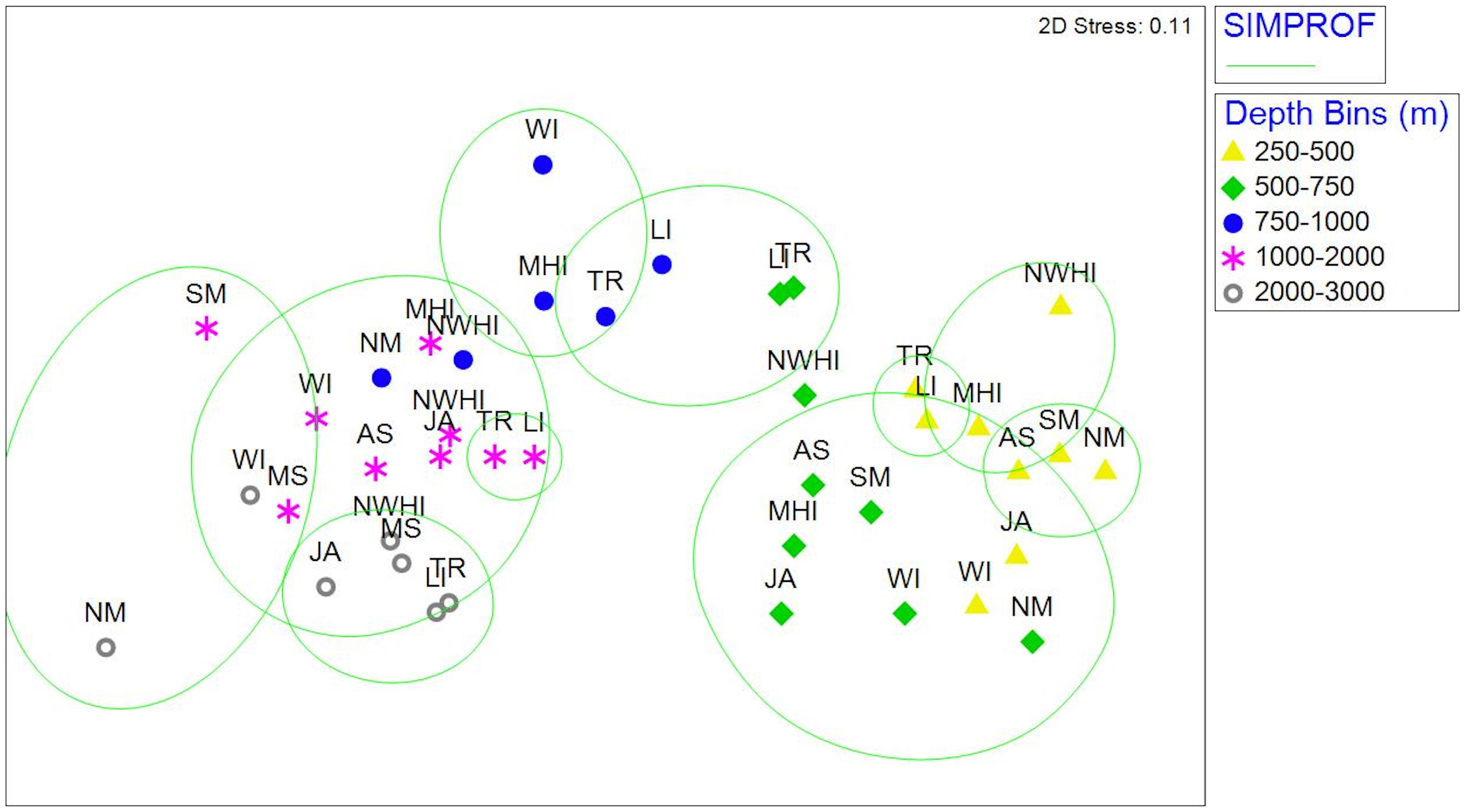
Figure 3 NMDS ordination based on Bray Curtis similarities calculated on square-root transformed and Wisconsin double standardized averaged abundances. Combined factors of region and depth bin (stress =0.11). Green ovals correspond to similar assemblages determined by SIMPROF analysis (SIMPROF, P<0.05). AS, American Samoa; JA, Johnston Atoll; LI, Line Islands; MHI, Main Hawaiian Islands; MS, Musicians Seamounts; NM, Northern Marianas; NWHI, Northwest Hawaiian Islands; SM, Southern Marianas; TR, Tokelau Ridge; WI, Wake Island.

Regional variation was also apparent as some regions clustered together in the upper and intermediate depth bins. The Line Islands and Tokelau Ridge between 250–1000 m and the Main Hawaiian Islands and Northwest Hawaiian Islands between 250–500 m had distinctly different assemblages compared to the rest of the regions (Figure 3).

Across all regions, there were more significantly different assemblages in the upper bathyal and intermediate depth bins indicating that there was more assemblage structure in the upper bathyal depths compared to the deep. The 250-500 m depth zone had the most regions that were statistically different and had a few regions that were different from one another despite being in relatively close geographic proximity. For instance, American Samoa was different from Tokelau Ridge just to its north and Johnston Atoll was different from the Main Hawaiian Islands and Northwest Hawaiian Islands despite being less than 1000 km away. Between 500-750 m, the number of regions that were different compared to the upper bathyal (250-500 m) was nearly cut in half. However, there were still differences between regions that were relatively close. American Samoa was still different from the Tokelau Ridge and Johnston Atoll was different from the Northwest Hawaiian Islands. The intermediate 750-1000 m depth bin has limitations for interpretation due to gaps in sampling; however, the Main Hawaiian Islands was different from the Line Islands and Tokelau Ridge. The deeper depth bins (1000-3000 m) had the least number of different regions. However, the statistical power available for samples from 2000-3000 m is hampered by no samples available in American Samoa and the Main Hawaiian Islands. Despite this limitation, Johnston Atoll was different from the Northwest Hawaiian Islands in the 2000-3000 m depth bin but not in the 1000-2000 m. Overall, the differences in assemblage structure covaried significantly with geographic distance in upper bathyal (250-500 m), intermediate (500-750, 750-1000 m) and deep (1000-2000, 2000-3000 m) depth strata (Mantel statistic: 250-500 m: 0.17, P = <0.001, 500-750 m: 0.27, P = <0.001, 750-1000 m: 0.23, P = <0.001, 1000-2000 m: 0.19, P= 0.001, 2000-3000 m: 0.13, P =0.001).

The regional differences in assemblage structure may be related to deep-sea water masses and their specific values of temperature, dissolved oxygen, salinity, and density. We identified six water individual masses across the ten sampling regions (WNPCW, NPIW, AAIW, NPDW, UCDW, LCDW, Supplementary Table 1) occurring in eight different combinations as some samples occurred at the nexus of two water masses and could not be differentiated (i.e., AAIW/NPIW, NPDW/LCDW, AAIW, UCDW). The intermediate depths encompassing American Samoa, Tokelau Ridge, Line Islands and Johnston Atoll, and the Main Hawaiian Islands are mainly occupied by Antarctic Intermediate Water (AAIW) whereas the Northwest Hawaiian Islands, Musicians Seamounts, Wake Island, and the Mariana Islands are mainly occupied by North Pacific Intermediate Water (NPIW/AAIW). Communities at sites that included WNPCW in the Main Hawaiian Islands, Northern Marianas, Southern Marianas, and Johnston Atoll were similar within 250-500 m. There were moderate similarities between assemblages in the NPIW/AAIW and AAIW within 500-1000 m. Overall, water mass generally followed depth strata with shallow samples on the far right, intermediate in the middle and deep samples on the far left (Supplementary Figure 3B).

3.3 Assemblage structure

In general, there were more upper bathyal assemblages compared to deep ones and a wider range in depths of assemblages in the upper bathyal regions compared to the deep (Table 4). Group average similarities ranged from 16% to 81%. The group that occurred in the most regions was group d (750-1000 m) which included samples from Johnston Atoll, Line Islands, Northern Marianas, Northwest Hawaiian Islands and Tokelau Ridge (21% similarity). The group with the highest similarity was group n (250-750 m) at 81% similarity which just included the Main Hawaiian Islands. Groups (250-500 m) at 16% just included American Samoa and had the least similar assemblages of all the assemblages. The large range in group average similarity may indicate limitations in the sample effort and or low spatial resolution. There were four assemblages that encompassed wide depth ranges between 250 and 1000 m and 13 assemblages that occurred between 250 and 750 m. There were only three assemblages that occurred strictly between 1000 and 3000 m. There were six assemblages in the upper bathyal and intermediate depths that occurred in only one region. These included the 250-500 m Line Island assemblage which were dominated by Chrionema (14.7% contribution), 250-500 m Main Hawaiian Islands assemblage (Owstonia, 31% contribution), 250-750 m Main Hawaiian Islands assemblage (Chascanopsetta, 22% contribution), 250-500 m Northern Marianas assemblage (Plectranthias, 23% contribution), 250-500 m American Samoa assemblage (Etelis, 70% contribution), and 500-750 m American Samoa assemblage (Phenacoscorpius, 90% contribution).

TABLE 4

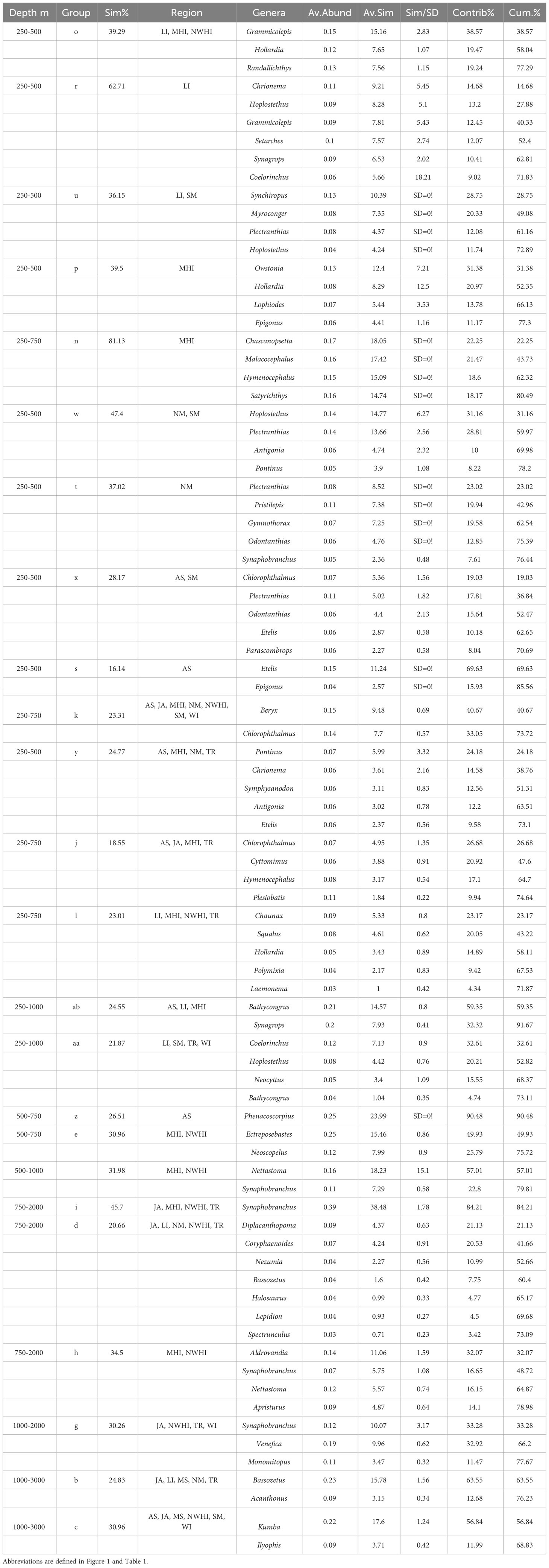
Table 4 List of genera that contribute most (70%; SIMPER) to similarity within the 24 fish assemblages identified by hierarchical analysis. .

3.4 The influence of environmental variables on assemblage structure

The environments of seamounts and oceanic islands are not homogenous as each have different physical, chemical, and geological characteristics with varying influence on fish assemblage structure. This pattern was observed as depth, dissolved oxygen, POC flux, and salinity together explained a total of 24% of the variation in assemblage structure (Figure 4, constrained proportion = 0.24). The first axis, CAP1, explained ~10% of the constrained variation (proportion explained = 0.09) and was strongly correlated with depth, moderately correlated with POC flux, and weakly correlated with concentrations of dissolved oxygen and salinity. POC flux varies in the opposite direction along this axis which was expected as POC flux generally declines with depth. The second axis, CAP2, explained ~4% of the constrained variation (proportion explained = 0.03) and has dissolved oxygen and POC flux occurring in opposite directions and little contribution from depth and salinity. The Line Islands and Tokelau Ridge had the highest POC flux values and lowest concentrations of dissolved oxygen and therefore may be driving this pattern on the CAP 2 axis. The influence of the environmental variables observed may also be driven by the structure of the different water masses found in the regions (Supplementary Table 1). Full ranges of environmental variables analyzed are provided in Supplementary Figure 1.

FIGURE 4

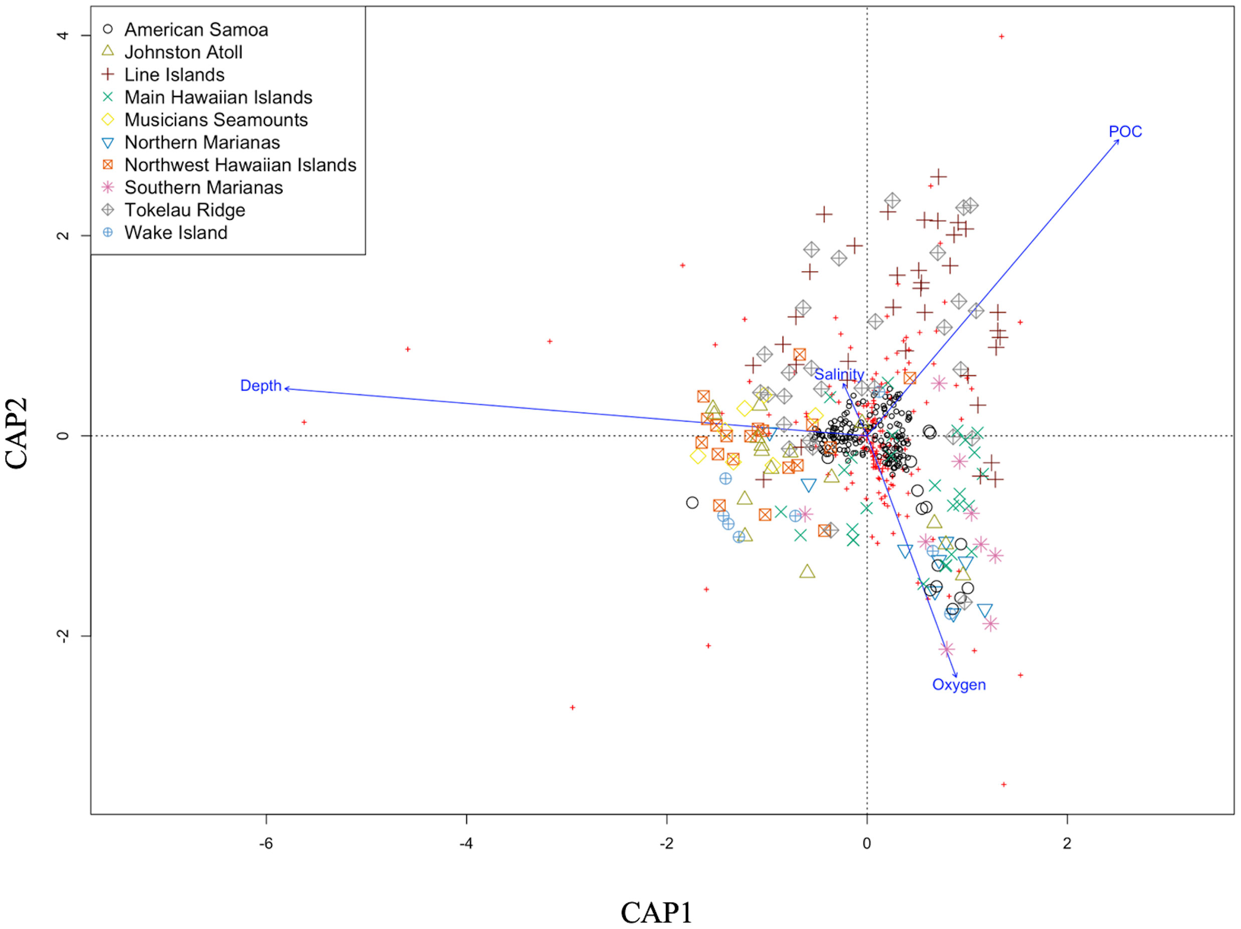
Figure 4 Canonical analysis of principle coordinates (CAP) based on Bray Curtis similarities calculated on Wisconsin transformed data (n = 212 samples). CAP1 explains 10% of the total variation while CAP2 explains 4%. The total constrained variation explained by all axes is 24%. CAP statistics generated by capscale in R. Colors=regions. Temperature was removed from the analysis as it was highly correlated to depth.

3.5 Total abundance

Total fish abundance generally decreased with depth across the regions. Samples with the lowest abundances (<0.01) occur mostly in the intermediate to deep depths, however the Main Hawaiian Islands and Tokelau Ridge had very high abundances between 750-1000 m (Figure 5), which were driven by the high abundance of Epigonidae and Setarchidae, respectively. Total abundance was greatest in the Line Islands between 250-500 m (6.05 fish/m) followed by the Northern Marianas between 250-500 m (4.42 fish/m). Changes in fish abundance with depth were significant in all regions (P = 0.001) except for the Musicians Seamounts (P = 0.9), with 75.1% of the deviance explained in the model.

FIGURE 5

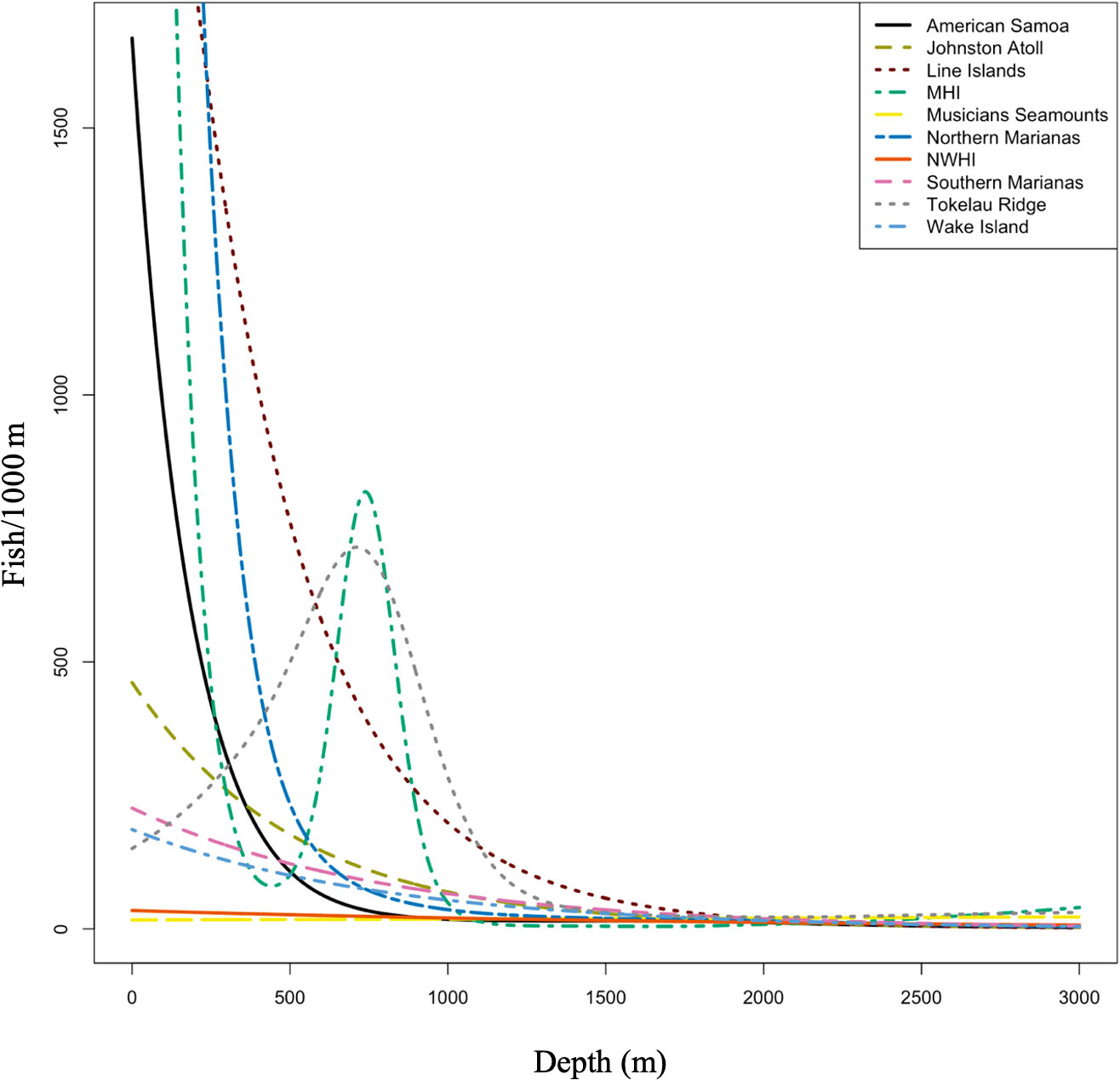
Figure 5 Smoothers (a parameter that controls the estimated predictive accuracy) in Generalized Additive Model (GAM) for total abundance (fish/km) by depth plotted by all regions. Changes in fish abundance with depth were significant in all regions (P= 0.001) except for the Musicians Seamounts (P = 0.9). MHI, Main Hawaiian Islands; NWHI, Northwest Hawaiian Islands.

3.6 Relationship between total abundance and environmental variables

Depth, concentrations of dissolved oxygen, POC flux, and salinity all had a significant relationship with fish abundance (fish/km) (P=0.001) and explained a little over 50% of the variation in total abundance (deviance explained =73.6%, generalized cross-validation score= 900). Total abundance was highest at depths of ~250 and ~725 m but then declined at ~1500 m (P=0.001). Dissolved oxygen was strongly related to abundance (P=0.001) where total abundance appeared highest between dissolved oxygen concentrations of 1.5 and 3.5 mg/L. Abundance increased with salinity, possibly due to water mass differences (Supplementary Figure 3); however, confidence intervals >34.5 are very large so this trend could be driven by a few observations with high salinity and high total abundance. For instance, the Line Islands 250-500 m sample bin had the highest salinity and abundance values. Fish abundance increased with increasing POC flux. In summary, fish abundances were predicted to be highest at the upper bathyal depths (250-500 m), with concentrations of dissolved oxygen between 1.5-3.5 mg/L, salinity values ~ 34.5, and POC flux values > 4 mg C/m²/day (Figure 6).

FIGURE 6

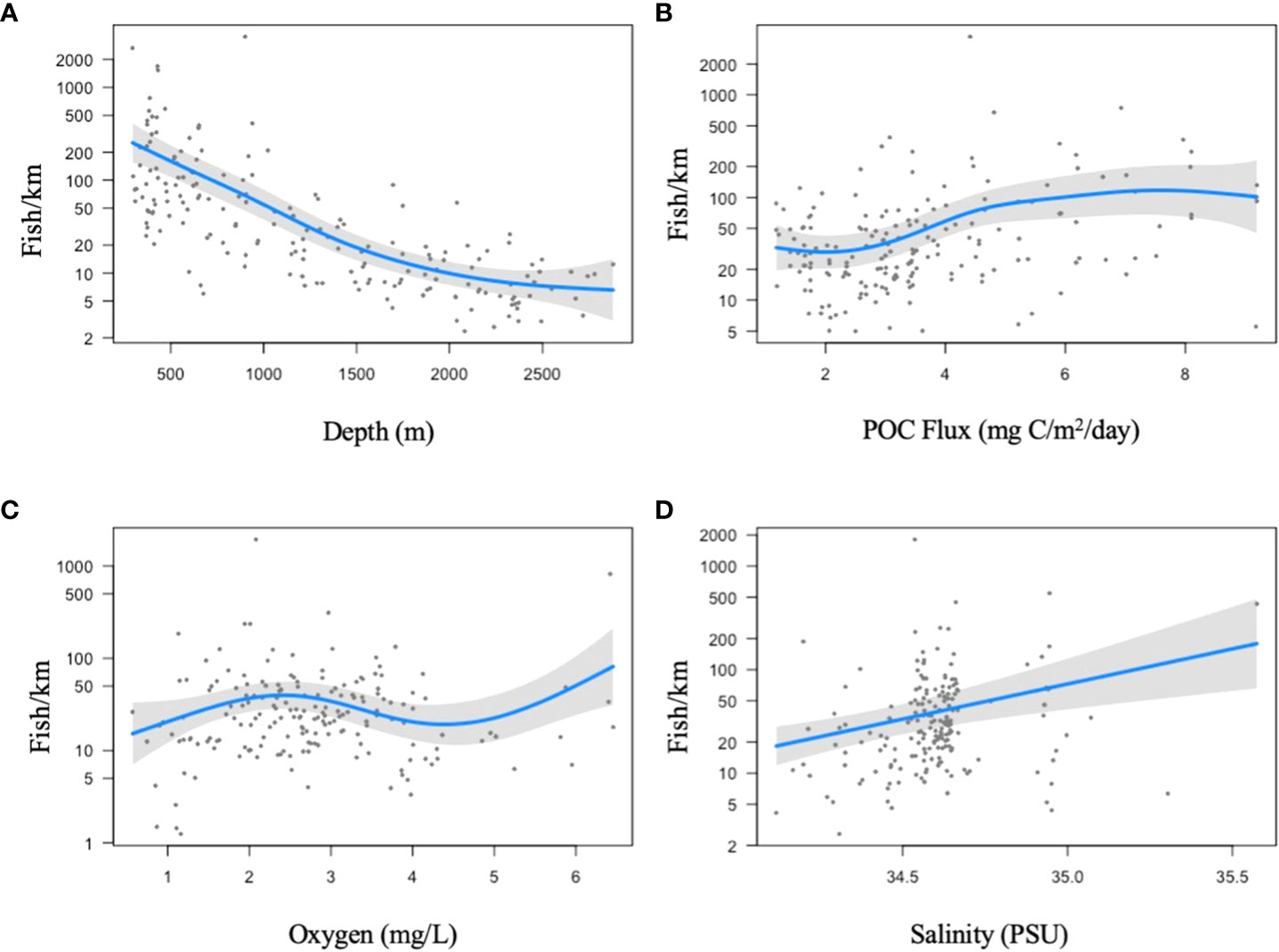
Figure 6 Generalized additive models (GAM) for total abundance (fish/km) in relation to (A) depth (m), (b) POC flux (mg C/m²/day), (C) dissolved oxygen (mg/l), and (D) Salinity (PSU) to the seafloor. Back transformed GAM functions with residuals. The spread of the data (y axis maxima) changed between plots because the plots show partial residuals and unexplained variation is added on top of the smoother. The shaded grey bands indicate confidence intervals on the standard deviation scale.

3.7 Diversity

There were not enough samples to generate curves based on region by depth bin, therefore, samples were parsed separately as region and depth. Rarefaction curves (Hill, q=0) were used to compare samples at the same sampling intensity (the same number of individuals) to determine whether generic richness differed between regions and depths. Extrapolation was included in the curves for reference but not used in comparisons. There were four regions with enough individuals (n = 2500) to compare at the same sampling intensity (the same number of individuals). These regions included the Northern Marianas, Line Islands, the Main Hawaiian Islands and Tokelau Ridge (Figure 7A). Out of these, Tokelau Ridge and the Main Hawaiian Islands had the highest estimated generic richness as these curves are well above the Line Islands and Northern Marianas curves. Results for samples parsed by depth bin indicated that deeper depths were far less sampled than upper bathyal locations (Figure 7B). The only depth bins with enough individuals (n = 2500) to compare at the same sampling intensity were 250-500 m and 500-750 m, which were closely aligned.

FIGURE 7

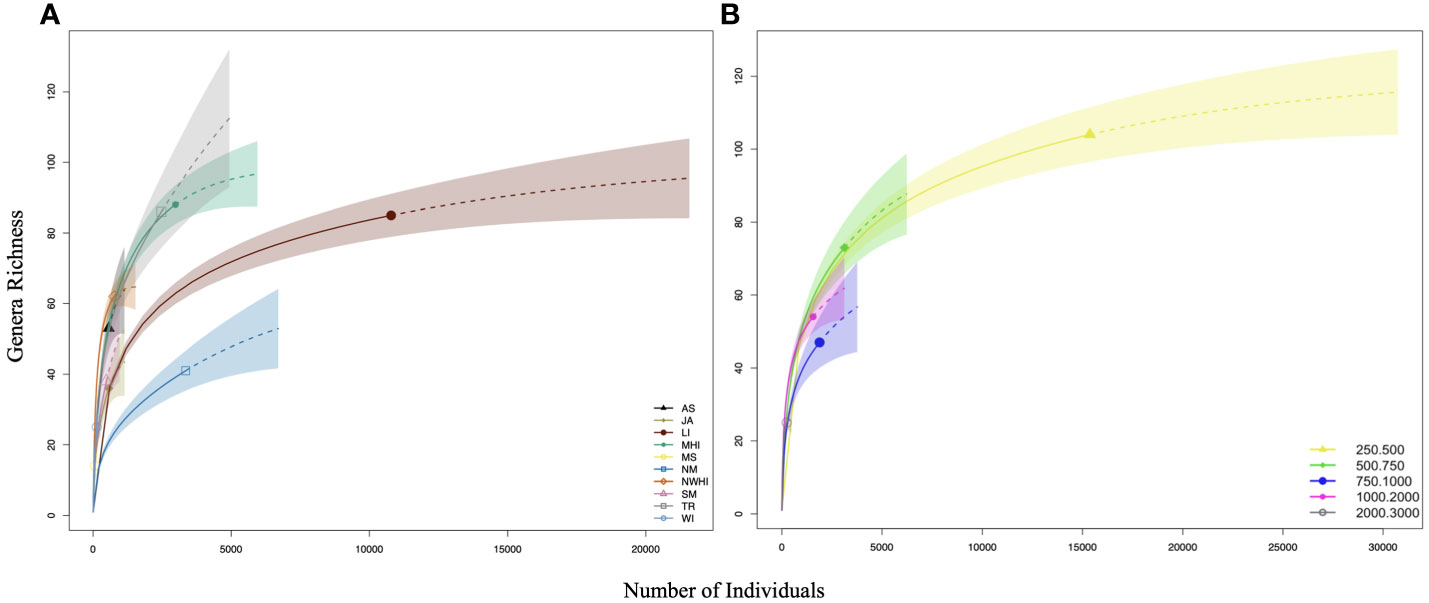
Figure 7 Rarefaction curves (by number of individuals) parsed by region and depth bin for estimating sampling effectiveness. (A, B) The top curves represent all regions and depths pooled, respectively. Extrapolations are indicated by dashed lines. Abbreviations are defined in Figure 1 and Table 1.

Chao 1 and Chao 2 were used to estimate generic richness based on samples rather than pooled individuals (limit of the rarefaction curves). Chao1 and 2 richness estimators predict higher richness for all regions and depths bins than the rarefaction extrapolation even for curves that are near asymptotes (LI and 250-500 m). In all Chao 1 and 2 cases, estimates exceed the number of genera collected indicating that there are still genera that remain uncollected. For example, Chao 1 and Chao 2 both estimate over 120 genera in the Northern Marianas, whereas only ~40 genera were collected (Supplementary Figures 2A, B). Similarly, Chao 1 and Chao 2 both estimate ~140 genera in 250-500 m, whereas only ~100 genera were collected, indicating that this depth bin is estimated to have the highest regional richness with many genera yet to be collected (Supplementary Figures 2C, D). There were six regions with enough samples (n = 10) to compare estimated generic richness at the same sampling intensity: Johnston Atoll, Northwest Hawaiian Islands, American Samoa, Main Hawaiian Islands, Line Islands, and Northern Marianas (Supplementary Figure 2A). Out of these, the Northern Marianas, followed by the Line Islands and Main Hawaiian Islands had the highest estimated generic richness (Supplementary Figure 2B). However, Chao 2 estimated the Main Hawaiian Islands to have the second highest generic richness. Results of Chao1 and 2 by depth bin indicated that there were enough samples to compare all depth bins at n = 10. Estimated generic richness generally was highest in the upper bathyal depth bins and decreased with depth. However, estimates of richness in the 500-750 m and 750-1000 m depth bins were more closely aligned in Chao 1 compared to Chao 2 (Supplementary Figures 2C, D).

The Line Islands, Main Hawaiian Islands, and Northern Marianas, and Tokelau Ridge had the lowest generic evenness (Pielou), with median index values under 0.75. The regions with the highest evenness were the Musicians Seamounts and the Northwest Hawaiian Islands (Figure 8A). When separating the data by depth bin, it becomes apparent that overall, evenness increased with depth. Although 750-1000 m has the lowest evenness value, 250-750 m are not far off, and the 2000-3000 m depth bin has the highest evenness value (Figure 8B).

FIGURE 8

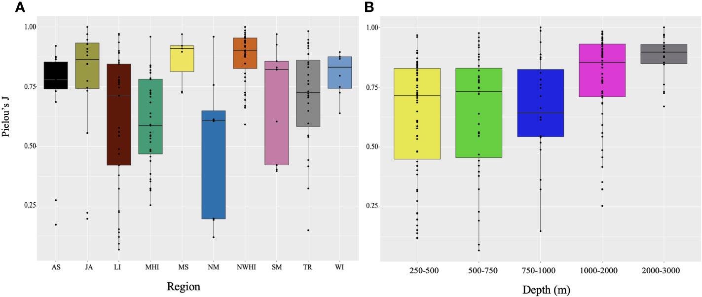
Figure 8 Boxplot of evenness values (Pielou’s J) for the genera observed parsed by (A) regions and (B) depth bins. Five summary statistics are displayed (median, two hinges, two whiskers, and all outlying points). Whiskers = minimum and maximum, box= lower and upper quartile, horizontal bold line = median. Abbreviations are defined in Figure 1 and Table 1.

4 Discussion

4.1 Patterns in assemblage structure

Comparisons of demersal fishes between regions in the central and western Pacific indicate that depth (and its correlates, temperature, and pressure) may play the most influential role in structuring assemblages. This was expected as depth zonation of demersal fishes is a common phenomenon in the deep-sea globally (Carney, 2005) and has been observed in other studies in the Pacific Ocean within the Hawaiian archipelago (Yeh and Drazen, 2009; De Leo et al., 2012). The reduction of light, temperature, dissolved oxygen, and food supply along with increasing pressure has been found to strongly influence the spatial distribution of species along with their functions and morphologies (Gallo and Levin, 2016). Despite some limited sampling at intermediate depths, assemblages became more similar with increasing depth. Deeper living fishes are also known to have wider distributions (resulting in increased similarities in assemblages) than upper bathyal fishes due to the increase in homogeneity and stabilization of environmental variables (Clark et al., 2010).

Regional separation was also apparent between assemblages suggesting that there are significant regional differences in the composition of demersal fauna across archipelagos in the central and western Pacific. The Main Hawaiian Islands and Northwest Hawaiian Islands had an upper bathyal assemblage (250-750 m) that was different from all other regions (Figure 5A). Shallow reef studies show that the Main Hawaiian Islands are characterized by a large number of endemic species (30% of inshore fishes) due to its geographic isolation (Hourigan and Reese, 1987). We suggest that Hawaii`s isolation may be causing its distinct upper bathyal fish assemblage. The genera that may be contributing to these differences in the upper bathyal zone include Owstonia, a bandfish genus that is found in the deep waters of the Indian and Pacific Ocean (Smith-Vaniz and Johnson, 2016) and Chascanopsetta, lefteye flounders with a tropical distribution from the Western Atlantic to the central Pacific (Hensley and Smale, 1997). Although we were unable to identify the majority of fishes beyond genera in the present analysis, our patterns could derive from patterns of endemic species similar to shallow reef environments. The Line Islands and Tokelau Ridge had an upper bathyal and intermediate assemblage (250-1000 m) that was different from all other regions (Figure 3) which align with studies that have found that neighboring regions harbor more similar fish assemblages (Clark et al., 2010). Also, these regions are within the equatorial upwelling zone with high productivity due to the dynamic seasonal changes in sea surface temperature (SST) and water column thermal and oxygen structure. Cold SST that is prevalent in equatorial waters during ENSO events like La Niña and shoaling of the thermocline and oxycline from enhanced upwelling may be creating a physiological barrier in these regions (Carlisle et al., 2017). The Line Islands and Tokelau Ridge had some of the lowest concentrations of dissolved oxygen and highest POC flux values, suggesting that these regions may be a biogeographic zone of faunal change. The center of the Pacific provinces as described in Watling et al. (2013) are within oligotrophic central gyres congruent with a zone of change near the equator. Further, a distinct change in mesopelagic fish fauna has been observed between two Equatorial components in the Pacific between a 14.5°N and 7°N (“north”) and 7°N and 3°S (“south”). Across these components, species adapted to low oxygen were observed in the north component and species adapted to high productivity were adapted to high productivity (Sutton et al., 2017). Faunal studies conducted across the postulated transition zone of the Equatorial and North Central Pacific provinces have observed significant changes in the diversity of mesopelagic fishes (Barnett, 1984; Clarke, 1987) as well as macrofaunal polychaetes and sediment-dwelling foraminiferans matching food availability at abyssal depths (Smith et al., 2008). Therefore, it’s possible that a similar transition zone may exist across the Equatorial and South Pacific, contributing to the changes observed in the demersal fish assemblage.

4.2 Relationship between assemblage structure and environmental gradients

Oxygen played a role in structuring central and western Pacific fish assemblages with the presence of low-oxygen zones from 250-1000 m in some regions. Persistent OMZs are likely to be important boundaries to species distributions and are hypothesized to be barriers to gene flow within populations in the deep sea (Rogers, 2000). Regional variation in the thickness and intensity of OMZs can be attributed to the differences in oceanographic currents, productivity, and aerobic respiration in the water column (Stramma et al., 2009). In the Hawaiian archipelago, there is a relatively weak OMZ between depths of 600 and 700 m with minimum oxygen concentrations of 0.84 mg/L at ~650 m (Yeh and Drazen, 2009; De Leo et al., 2012). Reduced fish abundances have been found there (De Leo et al., 2012). In the present study, very low concentrations of dissolved oxygen were found in several regions with the lowest concentrations of dissolved oxygen found in the Line Islands (minimum dissolved oxygen value of 0.56 mg/L), Johnston Atoll (minimum value of 0.75 mg/L), and Tokelau Ridge (minimum value of 1.3 mg/L, lowest values given rather than lowest sample averages). Although dissolved oxygen in the last two regions is higher than the threshold considered for oxygen minimum zones around the globe (0.7 mg/L, Gibson and Atkinson, 2003), and more characteristic of an oxygen minimum layer characterized as hypoxic (dissolved oxygen (DO < 2 mg/L) (Jaker et al., 2020), the low oxygen in all three regions could be acting as a physiological barrier to some genera.

Part of the variance in the assemblage structure of demersal fishes in the central and western Pacific can be attributed to POC flux, a proxy for food availability. Generally, POC flux decreases with depth and the distance from shore, the source of coastal nutrients, and vascular plant and macroalgae material. However, depth-related decrease in POC flux becomes more complicated with more complex bathymetry and where OMZs intersect continental margins and seamounts (Levin et al., 2001; De Leo et al., 2014). Both indirect and direct changes in food quantity and quality in deep-sea assemblages can alter food web structure, abundance, and diversity; therefore, it’s not surprising that POC flux values were correlated with the variation in assemblage structure across all regions. Deep-sea habitats generally have low biomass due to the low food availability, and reproduction and growth of fishes are all reduced with increasing depth which is likely related to both food supply and temperature (Levin et al., 2001). POC flux was highest in the Line Islands and Tokelau Ridge for all depths which also had some of the lowest oxygen levels. It’s likely that the low-oxygen environments in these OMZs are influencing material cycling in the region and the transfer of organic matter to deep waters (Ma et al., 2021). Further, surface waters in these regions may have higher biological productivity due to equatorial upwelling processes (Chavez and Messié, 2009).

Care is needed when interpreting the overall importance of environmental variables in governing assemblage structure. The first two axes in the CAP analysis combined accounted for ~14% of the variation, indicating that there are other predictors that explain the variation not included in the present study. Small-scale habitat variability has been found to contribute to the spatial variation of deep-sea fish assemblages (Auster et al., 2005) and notably among different slopes of the same seamount in the Northwest Hawaiian Islands (Mejía-Mercado et al., 2019). Other abiotic factors such as mesoscale oceanography, light intensity, and hydrostatic pressure along with biotic factors like competition, food web linkages, and parasitism may be contributing to the unexplained variation (Levin et al., 2001).

4.3 Relationship between total abundance and environmental gradients

Overall, total abundance was found to decrease with depth which is in alignment with the decrease in food input available for organisms inhabiting deeper depths and the physiological adaptations fishes have acquired for dealing with low food quantity and quality at depth (Cocker, 1978). An exponential decrease in fish abundance with depth has also been observed in oligotrophic areas of the Atlantic (Merrett et al., 1991). However, there were two exceptions to this general pattern in the Main Hawaiian Islands and Tokelau Ridge where there was a high abundance of fishes at ~750 m. This was driven primarily by two genera, Epigonus and Setarches. In a 2015 dive conducted during CAPSTONE (D2-EX1504L4-01), which took place just south of O`ahu (Main Hawaiian Islands), there was a high abundance of Epigonus. Similarly, in a 2017 dive conducted during CAPSTONE (D2-EX1703-08) which also took place on an island flank near Howland Island (Tokelau Ridge), there were a high abundance of Setarches. There is evidence of enhanced primary productivity within the Line Islands (Howland, Baker, and Jarvis Island) in relation to the central Pacific Ocean gyres to the north and south of the equator. Evidence suggests that enhancement and concentration of phytoplankton from equatorial upwelling occur in fronts at the leading and trailing edges of tropical waves in which chlorophyll concentrations have been found to be an order of magnitude greater than background levels (Maragos et al., 2008; Mundy et al., 2010). It’s possible that these high abundances are also driven by the enhancement of phytoplankton in near-island ecosystems known as the Island Mass Effect (IME). Although much yet remains unknown about the exact mechanisms causing this phenomenon, the increase in phytoplankton biomass in close proximities to island ecosystems has been documented for over half a century. Across the central and western Pacific, islands and atolls exposed to elevated levels of nearshore phytoplankton support higher fish biomass. However, IME strength can vary depending on the geomorphic type, bathymetric slope, and local human-derived nutrient input (Gove et al., 2016).

The relationship between total abundance and all environmental predictors (depth, concentrations of dissolved oxygen, POC flux, and salinity) was significant. Total abundance was predicted to be highest at upper bathyal depths between 250-500 m which is in accordance with the strong depth zonation patterns in fish assemblages that are linked with both biotic (competition, predation, and nutritional resource availability) and abiotic variables (substrate, temperature, light) that vary with depth (Scott et al., 2022). Total abundance increased with higher POC flux values which were generally highest in upper bathyal water as expected. However, it’s important to note that seafloor POC flux values were averaged across varying water column characteristics, therefore there may be regional differences that are unable to be captured by the POC flux model (Leitner et al., 2020). Further, organic matter may be underestimated, especially from human-derived runoff near islands (Gove et al., 2016). In addition to the positive relationship with POC flux, total abundance was found to be highest between dissolved oxygen values of 1.5 to 3.5 mg/L, however, sampling was limited where values were >4 mg/L. Many studies have found a general decrease in demersal fish density, biomass, or CPUE with decreasing oxygen levels, but the effect is nonlinear and there are greater reductions below certain oxygen thresholds which are region-specific and influenced by depth, temperature, and the demersal fauna inhabiting them (Gallo and Levin, 2016). In Hawai`i, where OMZ conditions are weak, there is a reduction in demersal fish abundances where oxygen conditions are lowest. In contrast, the regions with the lowest dissolved oxygen and highest values of benthic POC flux (Line Islands and Tokelau Ridge) had some of the highest average fish abundance values. Since there are limitations in the POC flux model’s ability to capture regional habitat variation, this relationship (and potential correlation with POC flux) is hard to disentangle. Total abundance was highest at salinity values ~34.6, however, the dynamic range of salinity is very small (34.1-36.2), therefore this pattern may not be ecologically relevant.

4.4 Diversity patterns

Although none of the regions were sampled adequately for a comprehensive comparison of diversity patterns, there were a few major trends that can be identified and linked to ecological theory. Overall, genera richness was found to decrease with depth and evenness to increase with depth. Trends in richness may be explained by the kinetic energy hypothesis which states that warmer temperatures in the upper bathyal zone may support higher diversity than cooler, deeper zones (Woolley et al., 2016). The decrease in richness with depth may also be explained by the more-individuals hypothesis which theorizes that higher energy availability promotes a higher number of individuals in an assemblage allowing more species to persist (Storch et al., 2018). Bottom-water oxygen availability could also be contributing to this phenomenon because the Line Islands, Tokelau Ridge, and Main Hawaiian Islands had some of the lowest oxygen concentrations and the highest richness. Habitat diversity may be added in these regions due to the weak, yet thick OMZ that is not present in the other regions. OMZs have been found to provide hypoxia-tolerant species refuge from non-tolerant species leading to changes in assemblage structure (Gallo and Levin, 2016). However, the high richness in these regions may also be due to the disproportionate sampling that was conducted in the upper bathyal depths, which is especially relevant for the Main Hawaiian Islands and Tokelau Ridge. The trend in evenness increasing with depth may be explained by fish species in deeper habitats being more uniformly abundant due to a reduced input of energy (Zintzen et al., 2017). Some studies on Atlantic seamounts (Perez et al., 2018; Victorero et al., 2018) find a similar pattern and have suggested that a few specialized species dominate shallow waters with high food availability, then evenness increases with depth as their dominance subsides. Also, it is easier to estimate evenness when there are more samples, so the greater sampling effort in the upper bathyal depths may be contributing to this trend. However, as Pielou’s evenness is not independent of richness, it’s important to consider that the upper bathyal samples were generally genera rich with more dominant species whereas deep samples had lower general richness but were more evenly distributed.

The present study includes the first published central and western Pacific records of a number of taxa. A prominent example is the first record of the family Oreosomatidae based on observations of a species of Neocyttus which resembles or may be the same as N. acanthorhynchus, otherwise known only from the western Indian ocean (Yearsley and Last, 1998). There were also the first observations of Halosaurus species in the central Pacific. The ROVs and submersibles did not have the capabilities to collect fish specimens during these surveys. Thus, physical specimens of Neocyttus were not collected to confirm the sightings despite compelling videographic evidence. However, Neocyttus and Halosaurus are known to be distributed in the New Zealand EEZ and Australia (McMillan et al., 2011). These new records and others emphasize the importance of exploration and the need for detailed follow-up studies in the central and western Pacific, especially at intermediate depths of 750–1000 m and past 3000 m.

4.5 Management implications and future considerations

This study has direct management implications as it demonstrates that there is clear regional variation in the demersal fish assemblages in the central and western Pacific. Our results clearly show that existing Marine National Monuments are complementary components of the regional diversity and harbor unique assemblages which highlights the need to maintain this broad network of protection. Nonetheless, there is still much to learn about the deep-sea and as our understanding of these habitats improves, many more threats to these environments are recognized. Therefore, the effectiveness of the Monuments will depend on the spatial distribution and depths of human-caused disturbances such as climate change, deep-sea mining, and fishing. For instance, there has already been an increase in the frequency of extreme El Niño and La Niña events which could lead to more physiological barriers and decreases in habitat availability (Carlisle et al., 2017). To get a better understanding of how these systems will be influenced by anthropogenic effects, we first need to get a complete characterization of the assemblages inhabiting the regions and gain greater clarity of the boundaries and gradients of faunal change.

Due to the sample resolution and study design, we did not investigate the relationships between assemblage structure and smaller scale habitat structure such as boulder fields, and larger seafloor features such as seamount summits, and submarine canyons. However, all of these have been found to influence deep-sea fish assemblage structure (Auster et al., 1995; Auster et al., 2005; Quattrini and Ross, 2006; Ross and Quattrini, 2007; Milligan et al., 2016; Leitner et al., 2020; Leitner et al., 2021). The present study provides a first look at these assemblages at a broader regional scale, but it is important to note that further studies should investigate assemblage structure at a finer scale to fully understand the ecological patterns.

5 Conclusions

This basin-wide analysis provides the first insight into the assemblage structure and distribution of deep-sea demersal fish fauna inhabiting the diverse island and seamount groups across the central and western Pacific. Depth was found to be important for structuring assemblages, which become more similar with depth. Fish assemblages of the Hawaiian archipelago and the Equatorial regions (Line Islands and Tokelau Ridge) were unique and are likely influenced by the presence of an OMZ, with high fish abundance likely caused by regionally high food availability (seafloor POC flux). The present analysis was made possible by significant exploratory survey results. Future studies could use the present work to inform sampling designs and increase sampling effort (especially at depths of 750–1000 m) to more systematically advance our knowledge of the variables (and spatial scales) driving the assemblage structure of fishes in the central and western Pacific. Additionally, studies need to collect specimens and identify taxa to the species level for greater insights into biogeographic patterns, especially in light of increasing anthropogenic activity in the deep sea (Glover and Smith, 2003).

Data availability statement

Publicly available datasets were analyzed in this study. This data can be found here: NOAA Deep Sea Coral Research and Technology Program (https://deepseacoraldata.noaa.gov/) and Hawaii Undersea Research Laboratory Archive (http://www.soest.hawaii.edu/HURL/HURLarchive/index.php).

Ethics statement

Ethical approval was not required for the study involving animals in accordance with the local legislation and institutional requirements because this study uses video recordings and no handling of animals was required.

Author contributions

GS analyzed all data and wrote manuscript. JD, BM, and PA contributed to methodological design, statistical advice, and writing. CK provided edits and critical information. All authors discussed the results and agree to be accountable for all aspects of the work. All authors contributed to the article and approved the submitted version.

Funding

This material is based upon work supported by the National Science Foundation Graduate Research. Fellowship Program under Grant No. (1842402 and 2236415).

Acknowledgments

The authors thank Kyle Edwards and Craig Smith for commenting on drafts and providing research advice. We also thank Meagan Putts, Sarah Bingo, Tiffany Bachtel, and Virginia Moriwake (University of Hawai`i at Manoa) for their video annotations, data compilation and assistance. John Caruso (emeritus, Tulane University, LA; TU); Dominique Didier (Millersville University, PA; no abbreviation); David Ebert (Moss Landing Marine Laboratories, CA; MLML); Mackenzie Gerringer (State University of New York Geneseo; no abbreviation); Brian Greene (Bernice P. Bishop Museum, HI; BPBM); Hsuan Ching (Hans) Ho (National Museum of Marine Biology & Aquarium, Taiwan; NMMBA); Tomio Iwamoto (emeritus, California Academy of Sciences, CA; CAS); John McCosker (California Academy of Sciences, CA, emeritus; CAS); Astrid Leitner (Monterey Bay Aquarium Research Institute, CA; MBARI); Douglas Markle (emeritus, Oregon State University, OR; OSU); Peter Rask Møller (Natural History Museum of Denmark, University of Copenhagen; NHMD); Jørgen Nielsen (emeritus, Natural History Museum of Denmark, University of Copenhagen; NHMD); Werner Schwarzhans (Natural History Museum of Denmark, University of Copenhagen; NHMD); Shinpei Ohashi (Hokkaido University, Japan; HUMZ); Andrea Quattrini (US National Museum of Natural History, DC; USNM); David G. Smith (emeritus, US National Museum of Natural History, DC; USNM); Kenneth Tighe (US National Museum of Natural History, DC; USNM); and Kenneth Sulak (emeritus, US Geological Survey, FL; USGS) assisted with identifications of fishes seen during the CAPSTONE expeditions. We thank David Riser (University of Connecticut) for his initial analysis of the CAPSTONE meta-data, Andrew Yool (National Oceanography Centre, UK), Les Watling, Mahany Lindquist (University of Hawai`i at Manoa), and Travis Washburn (Geological Survey of Japan, National Institute of Advanced Industrial Science and Technology, Japan) for their help with the POC flux modeling, and Marti Anderson (Massey University, New Zealand) for their statistical expertise. Finally, we thank the Ocean Exploration Trust (OET), NOAA Deep Sea Coral Research and Technology Program (DSCRTP), NMFS Pacific Islands Fisheries Science Center, and the Deep-sea Animal Research Center (DARC) for making this data available. This is Ocean Research Explorations contribution ORE-014, Hawaii Biological Survey contribution 2023-007, Pacific Biological Survey contribution 2023-003, and SOEST Contribution # 11733.

Conflict of interest

The authors declare that the research was conducted in the absence of any commercial or financial relationships that could be construed as a potential conflict of interest.

Publisher’s note

All claims expressed in this article are solely those of the authors and do not necessarily represent those of their affiliated organizations, or those of the publisher, the editors and the reviewers. Any product that may be evaluated in this article, or claim that may be made by its manufacturer, is not guaranteed or endorsed by the publisher.

Author disclaimer

Any opinions, findings, and conclusions or recommendations expressed in this material are those of the author(s) and do not necessarily reflect the views of the National Science Foundation.

Supplementary material

The Supplementary Material for this article can be found online at: https://www.frontiersin.org/articles/10.3389/fmars.2023.1219368/full#supplementary-material

References

Amorim P., Peran A. D., Pham C. K., Juliano M., Cardigos F., Tempera F., et al. (2017). Overview of the ocean climatology and its variability in the Azores region of the North Atlantic including environmental characteristics at the seabed. Front. Mar. Sci. 4. doi: 10.3389/fmars.2017.00056

CrossRef Full Text | Google Scholar

Auster P., Malatesta R., LaRosa S. (1995). Patterns of microhabitat utilization by mobile megafauna on the southern New England (USA) continental shelf and slope. Mar. Ecol. Prog. Series. 127, 77–85. doi: 10.3354/meps127077

CrossRef Full Text | Google Scholar

Auster P. J., Moore J., Heinonen K. B., Watling L. (2005). A habitat classification scheme for seamount landscapes: assessing the functional role of deep-water corals as fish habitat. Cold-water corals ecosys. 761, 769. doi: 10.1007/3-540-27673-4_40

CrossRef Full Text | Google Scholar

Barnett M. A. (1984). Mesopelagic fish zoogeography in the central tropical and subtropical Pacific Ocean: species composition and structure at representative locations in three ecosystems. Mar. Biol. 82, 199–208. doi: 10.1007/BF00394103

CrossRef Full Text | Google Scholar

Bergstad O. A., Menezes G., Høines Å.S. (2008). Demersal fish on a mid-ocean ridge: Distribution patterns and structuring factors. Deep Sea Res. Part II: Topical Stud. Oceanogr. 55:1-2, 185–202. doi: 10.1016/j.dsr2.2007.09.005

CrossRef Full Text | Google Scholar

Böhlke E. B. (1989). “Fishes of the western North Atlantic. Volume One: Orders Anguilliformes and Saccopharyngiformes,” in Memoirs of the Sears Foundation for Marine Research (Mem. I: Yale University Press), 104–206.

Google Scholar

Borcard D., Gillet F., Legendre P. (2011). Numerical ecology with R (New York: springer).

Google Scholar

Brito-Morales I., Schoeman D. S., Molinos J. G., Burrows M. T., Klein C. J., Arafeh-Dalmau N., et al. (2020). Climate velocity reveals increasing exposure of deep-ocean biodiversity to future warming. Nat. Climate Change. 10, 576–581. doi: 10.1038/s41558-020-0773-5

CrossRef Full Text | Google Scholar

Cantwell K. (2020). Cruise Report: EX-17-08, Deep-Sea Symphony: Exploring the Musicians Seamounts (ROV & Mapping) (United States: Office of Oceanic and Atmospheric Research; United States. National Oceanic and Atmospheric Administration. Office of Ocean Exploration and Research). doi: 10.25923/PVW9-B391

CrossRef Full Text | Google Scholar

Carlisle A. B., Kochevar R. E., Arostegui M. C., Ganong J. E., Castleton M., Schratwieser J., et al. (2017). Influence of temperature and oxygen on the distribution of blue marlin (Makaira nigricans) in the Central Pacific. Fish. Oceanogr. 26, 34–48. doi: 10.1111/fog.12183

CrossRef Full Text | Google Scholar

Carney R. S. (2005). “Zonation of deep biota on continental margins,” in Oceanography and Marine Biology – An annual review (CRC Press), 43, 211–278.

Google Scholar

Carpenter K. E., Niem V. H. (1999a). “The living marine resources of thewestern central Pacific,” in Batoid fishes, chimaeras and bony fishes part 1 (Elopidae toLinophrynidae) (Rome: FAO), 1398–2068.

Google Scholar

Carpenter K. E., Niem V. H. (1999b). “The living marine resources of thewestern central Pacific,” in Batoid fishes, chimaeras and bony fishes part 1 (Mugilidae toCarangidae) (Rome: FAO), 2069–2790.

Google Scholar

Carpenter K. E., Niem V. H. (2001a). “The living marine resources of thewestern central Pacific,” in Bony fishes part 3 (Menidae to Pomacentridae) (Rome: FAO), 2791–3380.

Google Scholar

Carpenter K. E., Niem V. H. (2001b). “The living marine resources of thewestern central Pacific,” in Bony fishes part 4 (Labridae to Latimeriidae), estuarinecrocodiles, sea turtles, sea snakes, and marine mammals (Rome: FAO), 3381–4218.

Google Scholar

Chao A., Gotelli N. J., Hsieh T. C., Sander E. L., Ma K. H., Colwell R. K., et al. (2014). Rarefaction and extrapolation with Hill numbers: A framework for sampling and estimation in species diversity studies. Ecol. Monogr. 84, 45–67. doi: 10.1890/13-0133.1

CrossRef Full Text | Google Scholar

Chave E. H., Mundy B. C. (1994). “Deep-sea benthic fish of the Hawaiian Archipelago, Cross Seamount, and Johnston Atoll,” in Pacific Science (University of Hawaii Press), 48, 367–409.

Google Scholar

Chavez F. P., Messié M. (2009). A comparison of eastern boundary upwelling ecosystems. Prog. Oceanogr. 83, 80–96. doi: 10.1016/j.pocean.2009.07.032

CrossRef Full Text | Google Scholar

Clark M. R., Althaus F., Williams A., Niklitschek E., Menezes G. M., Hareide N.-R., et al. (2010). Are deep-sea demersal fish assemblages globally homogenous? Insights from seamounts: Are deep-sea demersal fish assemblages globally homogenous? Mar. Ecol. 31, 39–51. doi: 10.1111/j.1439-0485.2010.00384.x

CrossRef Full Text | Google Scholar

Clarke T. A. (1987). The distribution of vertically migrating fishes across the central equatorial Pacific. Biol. Oceanogr. 4:1, 4781. doi: 10.1080/01965581.1987.10749484

CrossRef Full Text | Google Scholar

Clarke K. R., Gorley R. N. (2006). PRIMER v6: User Manual/Tutorial, Plymouth Routines in Multivariate Ecological Research. (Plymouth: PRIMER-E).

Google Scholar

Cocker J. E. (1978). doi: 10.1007/BF00000532

CrossRef Full Text | Google Scholar

Cohen D. M., Inada T., Iwamoto T., Scialabba N. (1990). “Gadiform fishes of the world,” in An annotated and illustrated catalogue of cods, hakes, grenad iers andother gadiform fishes known to date (Rome: FAO), 442.

Google Scholar

Colvocoresses J. A., Musick J. (1984). Species associations and community composition of middle Atlantic Bight continental-shelf demersal fishes. Fish. Bullet. 82, 295.

Google Scholar

Compagno L. J. V. (1984a). “Sharks of the world,” in An annotated and illustratedcatalogue of shark species known to date. Part 1. Hexanchiformes to Lamniformes (Rome: FAO), 1–249.

Google Scholar

Compagno L. J. V. (1984b). “Sharks of the world,” in An annotated and illustratedcatalogue of shark species known to date. Part 2. Carcharhiniformes (Rome: FAO), 251–655.

Google Scholar

De Leo F. C., Drazen J. C., Vetter E. W., Rowden A. A., Smith C. R. (2012). The effects of submarine canyons and the oxygen minimum zone on deep-sea fish assemblages off Hawai’i. Deep Sea Res. Part I: Oceanogr. Res. Pap. 64, 54–70. doi: 10.1016/j.dsr.2012.01.014

CrossRef Full Text | Google Scholar

De Leo F. C., Vetter E. W., Smith C. R., Rowden A. A., McGranaghan M. (2014). Spatial scale-dependent habitat heterogeneity influences submarine canyon macrofaunal abundance and diversity off the Main and Northwest Hawaiian Islands. Deep Sea Res. Part II: Topical Stud. Oceanogr. 104, 267–290. doi: 10.1016/j.dsr2.2013.06.015

CrossRef Full Text | Google Scholar

Drazen J. C., Leitner A. B., Jones D. O. B., Simon-Lledó E. (2021). Regional variation in communities of demersal fishes and scavengers across the CCZ and Pacific ocean. Front. Mar. Sci. 8. doi: 10.3389/fmars.2021.630616

CrossRef Full Text | Google Scholar

Emery W. J. (2001). “Water types and water masses,” in Encyclopedia of ocean sciences (Oxford: Academic Press), 3179–3187.

Google Scholar

Francis M. P., Hurst R. J., McArdle B. H., Bagley N. W., Anderson O. F. (2002). New Zealand demersal fish assemblages. Environ. Biol. Fish. 65, 215–234. doi: 10.1023/A:1020046713411

CrossRef Full Text | Google Scholar

Fujita T., Inada T., Ishito Y. (1995). Depth-gradient structure of the demersal fish community on the continental shelf and upper slope off Sendai Bay, Japan. Mar. Ecol. Prog. Series. 118, 13–23. doi: 10.3354/meps118013

CrossRef Full Text | Google Scholar

Galarza J. A., Carreras-Carbonell J., Macpherson E., Pascual M., Roques S., Turner G. F., et al. (2009). The influence of oceanographic fronts and early-life-history traits on connectivity among littoral fish species. Proc. Natl. Acad. Sci. 106, 1473–1478. doi: 10.1073/pnas.0806804106

CrossRef Full Text | Google Scholar

Gallo N. D., Levin L. A. (2016). “Fish Ecology and Evolution in the World’s Oxygen Minimum Zones and Implications of Ocean Deoxygenation,” in Advances in Marine Biology (Academic Press), 74, 117–198. doi: 10.1016/bs.amb.2016.04.001

CrossRef Full Text | Google Scholar

Gauch J. H., Whittaker R. H., Wentworth T. R. (1977). “A comparative study of reciprocal averaging and other ordination techniques,” the Journal of Ecology (British Ecological Society), 157–174. doi: 10.2307/2259071

CrossRef Full Text | Google Scholar

GEBCO Compilation Group. (2023). GEBCO 2023 Grid. Available at: https://www.gebco.net/data_and_products/gridded_bathymetry_data/ [Accessed September 15, 2022].

Google Scholar

Gibson R. N., Atkinson R. J. A. (2003). “Oxygen minimum zone benthos: adaptation and community response to hypoxia,” in Oceanography and Marine Biology: An Annual Review (CRC Press), 41, 1–45.

Google Scholar

Gilbert C. H. (1905). The deep-sea fishes of the Hawaiian Islands. Bull. US Fish Commun. 23, 577–713. doi: 10.5962/bhl.title.12624

CrossRef Full Text | Google Scholar

Glover A. G., Smith C. R. (2003). The deep-sea floor ecosystem: Current status and prospects of anthropogenic change by the year 2025. Environ. Conserv. 30, 219–241. doi: 10.1017/S0376892903000225

CrossRef Full Text | Google Scholar

Gove J. M., McManus M. A., Neuheimer A. B., Polovina J. J., Drazen J. C., Smith C. R., et al. (2016). Near-island biological hotspots in barren ocean basins. Nat. Commun. 7, 10581. doi: 10.1038/ncomms10581

PubMed Abstract | CrossRef Full Text | Google Scholar

Grothues T. M., Cowen R. K. (1999). Larval fish assemblages and water mass history in a major faunal transition zone. Continental Shelf Res. 19, 1171–1198. doi: 10.1016/S0278-4343(99)00010-2

CrossRef Full Text | Google Scholar

Haedrich R. L., Merrett N. R. (1990). Little evidence for faunal zonation or communities in deep sea demersal fish faunas. Prog. Oceanogr. 24, 239–250. doi: 10.1016/0079-6611(90)90033-X

CrossRef Full Text | Google Scholar

Hastie T., Tibshirani R. (2023). Generalized additive models: some applications. J. Am. Stat. Assoc. 82, 371–386. doi: 10.1080/01621459.1987.10478440

CrossRef Full Text | Google Scholar

Hensley D. A., Smale M. J. (1997). A new species of the flatfish genus Chascanopsetta (Pleuronectiformes: Bothidae), from the coasts of Kenya and Somaliawith comments on C. lugubris (South Africa: J.L.B. Smith Institute of Ichthyology Special Publication). 1–16.

Google Scholar

Hourigan T. F., Reese E. S. (1987). Mid-ocean isolation and the evolution of Hawaiian reef fishes. Trends Ecol. evol. 2, 187–191. doi: 10.1016/0169-5347(87)90018-8

PubMed Abstract | CrossRef Full Text | Google Scholar

Jaker H., Uddin S. A., Jing Z. (2020). Historical overview of hypoxia in the Bay of Bengal. J. East China Normal Univ. (Natural Sciences), 1, 109–113. doi: 10.3969/j.issn.1000-5641.202092218

CrossRef Full Text | Google Scholar

Kawabe M., Fujio S. (2010). Pacific Ocean circulation based on observation. J. Oceanogr. 66, 389–403. doi: 10.1007/s10872-010-0034-8

CrossRef Full Text | Google Scholar

Kelley C., Hourigan T., Raineault N. A., Balbas A., Wanless D., Marsh L., et al. (2019). Enigmatic seamounts exploring the geologic origins and biological assemblages in papahānaumokuākea marine national monument. Oceanography 32, 1.

Google Scholar

Kennedy B. R. C., Cantwell K., Malik M., Kelley C., Potter J., Elliott K., et al. (2019). The unknown and the unexplored: insights into the Pacific deep-sea following NOAA CAPSTONE expeditions. Front. Mar. Sci. 6. doi: 10.3389/fmars.2019.00480

CrossRef Full Text | Google Scholar

Khedkar G. D., Jadhao B. V., Khedkar C. D., Chavan N. V. (2003). “FISH| Demersal Species of Temperate Climates,” in Encyclopedia of Food Science and Nutrition (Netherlands: Academic Press), 2424–2428.

Google Scholar

Koslow J. A., Bulman C. M., Lyle J. M. (1994). The mid-slope demersal fish community off southeastern Australia. Deep Sea Res. Part I: Oceanogr. Res. Pap. 41, 113–141. doi: 10.1016/0967-0637(94)90029-9

CrossRef Full Text | Google Scholar

Labropoulou M., Papaconstantinou C. (2000). “Community structure of deep-sea demersal fish in the North Aegean Sea (northeastern Mediterranean),” in Island, Ocean and Deep-Sea Biology. Eds. Jones M. B., Azevedo J. M. N., Neto A. I., Costa A. C., Martins A. M. F. (Dordrecht: Springer), 281–296. Developments in Hydrobiology.

Google Scholar

Leitner A., Friedrich T., Kelley C., Travis S., Partridge D., Powell B., et al. (2021). Biogeophysical influence of large-scale bathymetric habitat types on mesophotic and upper bathyal demersal fish assemblages: A Hawaiian case study. Mar. Ecol. Prog. Ser. 659, 219–236. doi: 10.3354/meps13581

CrossRef Full Text | Google Scholar

Leitner A. B., Neuheimer A. B., Drazen J. C. (2020). Evidence for long-term seamount-induced chlorophyll enhancements. Sci. Rep. 10, 12729. doi: 10.1038/s41598-020-69564-0

PubMed Abstract | CrossRef Full Text | Google Scholar

Levin L. A., Etter R. J., Rex M. A., Gooday A. J., Smith C. R., Pineda J., et al. (2001). Environmental influences on regional deep-sea species diversity. Annu. Rev. Ecol. System. 32, 51–93. doi: 10.1146/annurev.ecolsys.32.081501.114002

CrossRef Full Text | Google Scholar

Lutz M. J., Caldeira K., Dunbar R. B., Behrenfeld M. J. (2007). Seasonal rhythms of net primary production and particulate organic carbon flux to depth describe the efficiency of biological pump in the global ocean. J. Geophys. Res.: Oceans 112 (C10). doi: 10.1029/2006JC003706

CrossRef Full Text | Google Scholar

Ma J., Song J., Li X., Wang Q., Zhong G., Yuan H., et al. (2021). The OMZ and its influence on POC in the tropical Western Pacific ocean: based on the survey in March 2018. Front. Earth Sci. 9. doi: 10.3389/feart.2021.632229

CrossRef Full Text | Google Scholar

Mahon R., Brown S. K., Zwanenburg K. C., Atkinson D. B., Buja K. R., Claflin L., et al. (1998). Assemblages and biogeography of demersal fishes of the east coast of North America. Can. J. Fish. Aquat. Sci. 55, 1704–1738. doi: 10.1139/f98-065

CrossRef Full Text | Google Scholar

Maragos J., Miller J., Gove J., De Martini E., Friedlander A. M., Godwin S., et al. (2008). “US Coral Reefs in the Line and Phoenix Islands, Central Pacific Ocean: History, Geology, Oceanography, and Biology,” in Coral Reefs of the USA. Coral Reefs of the World. Eds. Riegl B. M., Dodge R. E. (Springer, Dordrecht), 1, 595–641.

Google Scholar

McMillan P. J., Francis M. P., James G. D., Paul L. J., Marriott P. J., Mackay E. (2011). New Zealand fishes. Volume 1: A field guide to common species caught by bottom and midwater fishing. New Z. Aquat. Environ. Biodivers. Rep. No 68, 329.

Google Scholar

Mejía-Mercado B. E., Mundy B., Baco A. R. (2019). Variation in the structure of the deep-sea fish assemblages on Necker Island, Northwestern Hawaiian Islands. Deep Sea Res. Part I: Oceanogr. Res. Pap. 152, 103086. doi: 10.1016/j.dsr.2019.103086

CrossRef Full Text | Google Scholar

Menezes G. M., Rosa A., Melo O., Pinho M. R. (2009). Demersal fish assemblages off the Seine and Sedlo seamounts (northeast Atlantic). Deep Sea Res. Part II: Topical Stud. Oceanogr. 56, 2683–2704. doi: 10.1016/j.dsr2.2008.12.028

CrossRef Full Text | Google Scholar

Menezes G. M., Sigler M. F., Silva H. M., Pinho M. R. (2006). Structure and zonation of demersal fish assemblages off the Azores Archipelago (mid-Atlantic). Mar. Ecol. Prog. Ser. 324, 241–260. doi: 10.3354/meps324241

CrossRef Full Text | Google Scholar

Merrett N. R., Gordon J. D. M., Stehmann M., Haedrich R. L. (1991). Deep demersal fish assemblage structure in the Porcupine Seabight (eastern North Atlantic): slope sampling by three different trawls compared. J. Mar. Biol. Assoc. United Kingdom. 71, 329–358. doi: 10.1017/S0025315400051638

CrossRef Full Text | Google Scholar

Milligan R. J., Spence G., Roberts J. M., Bailey D. M. (2016). Fish communities associated with cold-water corals vary with depth and substratum type. Deep Sea Res. Part I: Oceanogr. Res. Pap. 114, 43–54. doi: 10.1016/j.dsr.2016.04.011

CrossRef Full Text | Google Scholar

Morato T., Bulman C., Pitcher T. J. (2009). Modelled effects of primary and secondary production enhancement by seamounts on local fish stocks. Deep Sea Res. Part II: Topical Stud. Oceanogr. 56, 2713–2719. doi: 10.1016/j.dsr2.2008.12.029

CrossRef Full Text | Google Scholar

Mundy B. C. (2005). “Checklist of the fishes of the Hawaiian archipelago,” Bishop Museum Bulletins in Zoology. (Hawaii: Bishop Museum Press).

Google Scholar

Mundy B. C., Wass E. D., Greene B., Zgliczynski B., Schroeder R. E., Musberger C. (2010). Inshore fishes of Howland island, Baker island, Jarvis island, Palmyra atoll, and Kingman reef. Atoll Res. Bull. 585, 1–133.

Google Scholar

Nakamura I., Parin N. V. (1993). “Snake mackerels and cutlassfishes of theworld (Families Gempylidae and Trichiuridae),” in An annotated and illustratedcatalogue of the snake mackerels, snoeks, excolars, gemfishes, sackfishes, domine,oilfish, cutlassfishes, scabbardfishes, hairtails, and frostfishes known to date (Rome: FAO), 1–136.

Google Scholar

Nielsen J. G., Cohen D. M., Markle D. F., Robins C. R. (1999). “Ophidiiformfishes of the world,” in An annotated and illustrated catalogue of pearlfishes, cusk-eels,brotulas and other ophidiiform fishes known to date (Rome: FAO), 178.

Google Scholar

Oksanen J., Blanchet F., Kind R., Legendre P., Minchin P., O’hara R., et al. (2016). Vegan: Community Ecology Package. R Package Version 2.3-4. Available at: https://github.com/vegandevs/vegan [Accessed September 20, 2022].

Google Scholar

Oyafuso Z. S., Drazen J. C., Moore C. H., Franklin E. C. (2017). Habitat-based species distribution modelling of the Hawaiian deepwater snapper-grouper complex. Fish. Res. 195, 19–27. doi: 10.1016/j.fishres.2017.06.011

CrossRef Full Text | Google Scholar

Palevsky H. I., Doney S. C. (2018). How choice of depth horizon influences the estimated spatial patterns and global magnitude of ocean carbon export flux. Geophys. Res. Letters. 45, 4171–4179. doi: 10.1029/2017GL076498

CrossRef Full Text | Google Scholar

Parin N. V. (1991). Fish fauna of the Nazca and Sala y Gomez submarine ridges, the easternmost outpost of the Indo-West Pacific zoogeographic region. Bull. Mar. Sci. 49, 671–683.

Google Scholar

Parin N. V., Mironov A. N., Nesis K. N. (1997). “Biology of the Nazca and Sala y Gòmez Submarine Ridges, an Outpost of the Indo-West Pacific Fauna in the Eastern Pacific Ocean: Composition and Distribution of the Fauna, its Communities and History,” in Advances in Marine Biology. (Academic Press), 32, 145–242.

Google Scholar

Parra H. E., Pham C. K., Menezes G. M., Rosa A., Tempera F., Morato T. (2017). Predictive modeling of deep-sea fish distribution in the Azores. Deep Sea Res. Part II: Topical Stud. Oceanogr. 145, 49–60. doi: 10.1016/j.dsr2.2016.01.004

CrossRef Full Text | Google Scholar

Perez J. A. A., Kitazato H., Sumida P. Y. G., Sant’Ana R., Mastella A. M. (2018). Benthopelagic megafauna assemblages of the Rio Grande rise (SW atlantic). Deep Sea Res. Part I: Oceanogr. Res. Pap. 134, 1–11. doi: 10.1016/j.dsr.2018.03.001

CrossRef Full Text | Google Scholar

Pielou E. C. (1966). The measurement of diversity in different types of biological collections. J. Theor. Biol. 13, 131–144. doi: 10.1016/0022-5193(66)90013-0

CrossRef Full Text | Google Scholar

Pitcher T. J., Morato T., Hart P. J. B., Clark M. R., Haggan N., Santos R. S. (2008). Seamounts: Ecology, Fisheries & Conservation (Australia: Blackwell Publishing Ltd). doi: 10.1002/9780470691953

CrossRef Full Text | Google Scholar

Putts M., Parrish F., Trusdell F., Kahng S. (2019). Structure and development of Hawaiian deep-water coral communities on Mauna Loa lava flows. Mar. Ecol. Prog. Series. 630, 69–82. doi: 10.3354/meps13106

CrossRef Full Text | Google Scholar

Quattrini A. M., Demopoulos A. W. J., Singer R., Roa-Varon A., Chaytor J. D. (2017). Demersal fish assemblages on seamounts and other rugged features in the northeastern Caribbean. Deep Sea Res. Part I: Oceanogr. Res. Pap. 123, 90–104. doi: 10.1016/j.dsr.2017.03.009

CrossRef Full Text | Google Scholar

Quattrini A. M., Ross S. W. (2006). Fishes associated with North Carolina shelf-edge hardbottoms and initial assessment of a proposed marine protected area. Bull. Mar. Sci. 79, 137–163.

Google Scholar

Richards W. J., McGowan M. F., Leming T., Lamkin J. T., Kelley S. (1993). Larval fish assemblages at the Loop Current boundary in the Gulf of Mexico. Bull. Mar. Sci. 53, 475–537.

Google Scholar

Rogers A. D. (2000). The role of the oceanic oxygen minima in generating biodiversity in the deep sea. Deep Sea Res. Part II: Topical Stud. Oceanogr. 47, 119–148. doi: 10.1016/S0967-0645(99)00107-1

CrossRef Full Text | Google Scholar

Ross S. W., Quattrini A. M. (2007). The fish fauna associated with deep coral banks off the southeastern United States. Deep Sea Res. Part I: Oceanogr. Res. Pap. 54, 975–1007. doi: 10.1016/j.dsr.2007.03.010

CrossRef Full Text | Google Scholar

Scott M. E., Tebbett S. B., Whitman K. L., Thompson C. A., Mancini F. B., Heupel M. R., et al. (2022). Variation in abundance, diversity and composition of coral reef fishes with increasing depth at a submerged shoal in the northern Great Barrier Reef. Rev. Fish Biol. Fish. 32, 941–962. doi: 10.1007/s11160-022-09716-9

CrossRef Full Text | Google Scholar

Smith C., Deleo F., Bernardino A., Sweetman A., Arbizu P. (2008). Abyssal food limitation, ecosystem structure and climate change. Trends Ecol. Evol. 23, 518–528. doi: 10.1016/j.tree.2008.05.002

PubMed Abstract | CrossRef Full Text | Google Scholar

Smith-Vaniz W. F., Johnson G. D. (2016). Hidden diversity in deep-water bandfishes: Review of Owstonia with descriptions of twenty-one new species (Teleostei: Cepolidae: Owstoniinae). Zootaxa 4187, 1. doi: 10.11646/zootaxa.4187.1.1

CrossRef Full Text | Google Scholar

Storch D., Bohdalková E., Okie J. (2018). The more-individuals hypothesis revisited: The role of community abundance in species richness regulation and the productivity-diversity relationship. Ecol. Letters. 21, 920–937. doi: 10.1111/ele.12941

CrossRef Full Text | Google Scholar

Stramma L., Visbeck M., Brandt P., Tanhua T., Wallace D. (2009). Deoxygenation in the oxygen minimum zone of the eastern tropical North Atlantic. Geophys. Res. Letters. 36, 20. doi: 10.1029/2009GL039593

CrossRef Full Text | Google Scholar

Struhsaker P. (1973). A contribution to the systematics and ecology of Hawaiian bathyal fishes. Ph.D dissertation. (University of Hawaii).

Google Scholar

Sutton T. T., Clark M. R., Dunn D. C., Halpin P. N., Rogers A. D., Guinotte J., et al. (2017). A global biogeographic classification of the mesopelagic zone. Deep Sea Res. Part I: Oceanogr. Res. Pap. 126, 85–102. doi: 10.1016/j.dsr.2017.05.006

CrossRef Full Text | Google Scholar

Tapia-Guerra J. M., Mecho A., Easton E. E., Gallardo M.D.L.Á., Gorny M., Sellanes J. (2021). First description of deep benthic habitats and communities of oceanic islands and seamounts of the Nazca Desventuradas Marine Park, Chile. Sci. Rep. 11, 6209. doi: 10.1038/s41598-021-85516-8

PubMed Abstract | CrossRef Full Text | Google Scholar

Tracey D. M., Bull B., Clark M. R., MaCkay K. A. (2004). Fish species composition on seamounts and adjacent slope in New Zealand waters. New Z. J. Mar. Freshw. Res. 38, 163–182. doi: 10.1080/00288330.2004.9517226

CrossRef Full Text | Google Scholar

Victorero L., Robert K., Robinson L. F., Taylor M. L., Huvenne V. A. (2018). Species replacement dominates megabenthos beta diversity in a remote seamount setting. Sci. Rep. 8, 4152. doi: 10.1038/s41598-018-22296-8

PubMed Abstract | CrossRef Full Text | Google Scholar

Watling L., Guinotte J., Clark M. R., Smith C. R. (2013). A proposed biogeography of the deep ocean floor. Prog. Oceanogr. 111, 91–112. doi: 10.1016/j.pocean.2012.11.003

CrossRef Full Text | Google Scholar

Woolley S. N., Tittensor D. P., Dunstan P. K., Guillera-Arroita G., Lahoz-Monfort J. J., Wintle B. A., et al. (2016). Deep-sea diversity patterns are shaped by energy availability. Nature 533, 393–396. doi: 10.1038/nature17937

PubMed Abstract | CrossRef Full Text | Google Scholar

Yearsley G. K., Last P. R. (1998). Neocyttus psilorhynchus, a new oreosomatid (Pisces, Zeiformes) from southern Australia and New Zealand, with redescriptions of its congeners. New Z. J. Mar. Freshw. Res. 32, 555–579. doi: 10.1080/00288330.1998.9516845

CrossRef Full Text | Google Scholar

Yeh J., Drazen J. C. (2009). Depth zonation and bathymetric trends of deep-sea megafaunal scavengers of the Hawaiian Islands. Deep Sea Res. Part I: Oceanogr. Res. Pap. 56, 251–266. doi: 10.1016/j.dsr.2008.08.005

CrossRef Full Text | Google Scholar

Zintzen V., Anderson M. J., Roberts C. D., Harvey E. S., Stewart A. L. (2017). Effects of latitude and depth on the beta diversity of New Zealand fish communities. Sci. Rep. 7, 8081. doi: 10.1038/s41598-017-08427-7

PubMed Abstract | CrossRef Full Text | Google Scholar