Dispersion of deep-sea hydrothermal plumes at the Endeavour Segment of the Juan de Fuca Ridge: a multiscale numerical study

A multiscale numerical framework has been developed to investigate the dispersion of deep-sea hydrothermal plumes that originate from the Endeavour Segment of the Juan de Fuca Ridge located in the Northeast Pacific. The analysis of simulation outputs presented in this study provides insights into the influences of tidal forcing and the buoyancy flux associated with hydrothermal venting on ocean circulation and plume dispersion in the presence of pronounced seafloor topography. The results indicate that tidal forcing drives anti-cyclonic circulation near the ridge-axis, while hydrothermal venting induces cyclonic circulation around vent fields within the axial rift valley. Tidal forcing has a notable impact on plume dispersion, particularly near the large topographic features to the north of the Endeavour Segment. Furthermore, plume dispersion exhibits notable inter-annual variability, with a northbound trajectory in 2016 and a southbound trajectory in 2021. The study also reveals that both buoyancy fluxes and tidal forcing enhance the mixing of hydrothermal plumes with ambient seawater.

1 Introduction

Hydrothermal discharge from volcanically hosted submarine vents plays a crucial role in the transfer of heat from the Earth’s interior and the release of essential chemicals that impact ocean and atmospheric biogeochemistry (German and Seyfried, 2014). These vents are also home to unique ecosystems that are fuelled mainly by geothermal and geochemical energy, decoupled from the photosynthesis that sustains the majority of life on the planet. Because of their remote locations, however, such vents remain chronically under-investigated and new and profound discoveries about their significance on a global scale continue apace. Only in the past decade, for example, has sustained exploration revealed the significance of hydrothermal vents as sources of iron (Fe) that can stimulate primary productivity and draw-down of CO₂ from the atmosphere (Resing et al., 2015; Jenkins et al., 2020). These recent discoveries – that hydrothermal plumes enriched in Fe and Mn can persist for thousands of kilometres away from ridge-axis sources (Gartman and Findlay, 2020) – challenge the long-standing view that these trace metals are mostly removed from hydrothermal solution through oxidation near their vent sources (German et al., 1991; Field and Sherrell, 2000). Despite ongoing deep-sea explorations, our understanding of the dispersion of hydrothermal materials from their sources into the ocean remains limited. This is largely due to the difficulty in directly observing the dispersion and evolution of hydrothermal plumes with sufficient spatial coverage and resolution.

The physical structure of a deep-sea hydrothermal plume can be divided into two parts: the buoyant stem and the non-buoyant cap (Lupton, 1995). The former refers to the portion of the plume that has positive buoyancy compared to ambient seawater. This buoyant stem of the plume originates from the source vent and expands outward, akin to an inverted cone, as it rises. On the other hand, the plume’s non-buoyant cap is in density equilibrium with the surrounding water column; therefore, instead of continuing to rise, the non-buoyant hydrothermal fluid spreads laterally along isopycnic surface and can travel far from the source vent while maintaining distinct geochemical signatures. The dynamics and transition between the buoyant stem and non-buoyant cap occur over a broad range of spatial and temporal scales. For example, turbulence within the buoyant stem can range from a few centimetres close to the vent orifice to tens of meters when the rising fluid reaches density equilibrium with the surrounding water column, hundreds of meters above the seafloor (e.g., Speer and Marshall, 1995). This process of fluid ascent in the buoyant stem typically takes no longer than 1 hour regardless of ocean stratification (Lupton, 1995). In contrast, the dispersion of the non-buoyant cap, which begins at its juncture with the buoyant stem and continues until its geochemical signature is indistinguishable from the ambient seawater, occurs on much larger spatial scales (e.g., thousands of kilometres) and over extended periods of time (e.g., years to decades). Additionally, the flow within the buoyant stem of a hydrothermal plume is primarily determined by the source heat flux and the ambient stratification. In comparison, the dynamics inside the non-buoyant cap are dominated by the ambient ocean circulation. A comprehensive investigation of these multi-scale, multi-disciplinary processes with direct field measurements is technically challenging and requires a combination of ship- and AUV-based surveys. Within the on-going US GEOTRACES program, ship-based surveys have been used to investigate the geochemical impacts of hydrothermal venting through the study of hydrothermal plumes’ dispersing non-buoyant caps at length scales of 100 km to 1000 km away from source vents (Resing et al., 2015; Jenkins et al., 2020). By contrast, AUV-based surveys offer the opportunity to study plume dispersion over 1 to 10 to 100km length scales (German et al., 2008; German et al., 2010). Even so, the implementation time for a coordinated AUV-based survey strategy may be long compared to the timescales of variability in plume dispersion close to a vent-source.

Consequently, achieving the spatial resolution required to reveal the complex (physical and biogeochemical) structures of such plumes remains challenging.

Numerical modelling has proven to be a valuable tool for investigating the physical evolution of hydrothermal discharge and the dispersal of vent larvae and chemicals near ocean ridges. Previous studies, such as those by Thomson et al. (2005); Thomson et al. (2009); Lavelle et al. (2010); Lavelle et al. (2013); Xu et al. (2018), and Vic et al. (2018), have demonstrated the effectiveness of numerical models in providing synoptic realizations of the dispersion of hydrothermally sourced materials in dynamic ocean-ridge environments. One notable example is the numerical study of the dispersal of hydrothermal Fe from the Mid-Atlantic Ridge (MAR) (Tagliabue et al., 2022). That study highlights the importance of incorporating sufficient spatial resolution to accurately represent dispersal processes over pronounced and variable ridge topography. Here, we investigate the dispersion of hydrothermal plumes from active vent sites on the Endeavour Segment of the Juan de Fuca Ridge (JDFR) through three-dimensional (3-D), multi-scale hydrodynamical simulations. In Section 2, we provide an overview of previous observations and modelling efforts related to ocean circulation and hydrothermal discharge at the Endeavour Segment. Section 3 details the configuration of our multi-scale modelling framework, and in Section 4 we present validation of our modelling approach in the form of a comparison with concurrent measurements of near-bottom flow velocity and observations from previous ship-based plume surveys. In Section 5, we describe the main simulation results and discuss the impact of various ocean processes on plume dispersion. Finally, we summarize our findings in Section 6.

2 Endeavour Segment, Juan de Fuca Ridge: hydrothermal vents, hydrography, and circulation

The Endeavour Segment of the Juan de Fuca Ridge (JDFR) is an intermediate rate spreading center located approximately 300 km offshore of British Columbia, Canada and Washington State, USA. The central portion of the 90 km long segment is a volcanic high dissected by a rift valley that is 100 – 200 m deep and 1 – 2 km wide. The axis of the valley is oriented along a heading of 020°T (relative to True North). Within the rift valley, there are at least five major hydrothermal vent fields, situated along the ridge axis, as well as multiple low-temperature discharge (i.e., diffuse flow) sites. The five major vent fields are: Mothra, Main Endeavour Field (MEF), High Rise (HR), Salty Dawg, and Sasquatch, listed from south to north (Figure 1). According to Kellogg and McDuff (2010), who conducted systematic hydrographic surveys using an AUV, the total hydrothermal heat flux from the axial valley is up to 900 MW, which makes Endeavour one of the most active second-order ridge segments known, worldwide (Kelley et al., 2012). The relative heat contributions from the five major hydrothermal fields are: Mothra (15%), MEF (34%), HR (43%), Salty Dawg (8%), and Sasquatch (<1%) (Kellogg, 2011). Seismic imaging has revealed magma bodies under all five major hydrothermal fields, suggesting that the vigorous venting at Endeavour is primarily driven by the heat output from the underlying magma chamber (Van Ark et al., 2007; Carbotte et al., 2012).

FIGURE 1

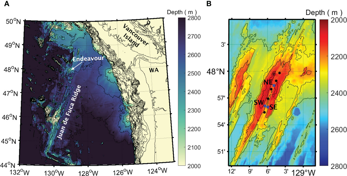
Figure 1 (A) Bathymetric maps of the JDFR in the Northeast Pacific, offshore Vancouver Island and Washington State (WA). The Endeavour Segment is located at the northern end of the ridge. (B) An expanded view of the Endeavour Segment, showing the rift valley that divides the central portion of the segment and the locations of the five major hydrothermal vent fields (black dots). From south to north, these vent fields are Mothra, MEF, HR, Salty Dawg, and Sasquatch. Three cabled current-meter moorings (RCM-NE, RCM-SW, RCM-SE) are denoted by blue squares and labeled NE, SW, and SE, respectively. Bathymetric data are from the Global Multi-Resolution Topography (GMRT) Synthesis of the Marine Geoscience Data System (Ryan et al., 2009).

Observations from ship-based water-column surveys have revealed the presence of a non-buoyant plume cap at ~2000-2100 m depth, i.e., approximately 100 – 200 m above the source vent fields on the Endeavour Segment. This non-buoyant plume cap disperses along the 27.7 $kg/m^3$ potential density anomaly (${\text{σ}}_{\text{θ}}$) surface, and its thermal and particulate signatures have been traced for more than 15 km away from the ridge-crest vents, downstream along the prevailing southwest current flow direction (Baker and Massoth, 1987; Thomson et al., 1992). Previous studies reported a southwestward mean flow along the ridge axis immediately above the axial valley (Baker and Massoth, 1987; Thomson et al., 2003). Current-meter moorings deployed along the Endeavour Segment, however, have recorded a more complex, time-varying pattern of circulation close to the ridge axis, characterized by distinct vertical and horizontal structures generated from interactions between large-scale abyssal flow, oscillatory currents, and the topography of the ridge axis (Thomson et al., 2003). Circulation within the axial valley is further influenced by dynamics driven by the buoyancy fluxes associated with hydrothermal venting. Close to the valley floor, the flow is directed into the valley from its northern and southern ends. The strength of this inflow is skewed towards the south, resulting in persistent northward flow from the southern end well past the middle of the valley (Thomson et al., 2003). Hydrothermal venting is thought to be the mechanism that draws flow into the valley through turbulent entrainment into rising buoyant plumes (Thomson et al., 2003). This hypothesis is supported by the findings of numerical simulations (Thomson et al., 2005; Thomson et al., 2009). Superimposed on this mean circulation pattern are oscillatory currents at a range of frequencies, including the semidiurnal (~12 hr), diurnal (~24 hr), near-inertial (~16 hr), and a low-frequency ‘weather’ band with a broad spectral peak around 4 to 6-day periods (e.g., Cannon and Thomson, 1996; Thomson et al., 2003). These currents are amplified near the ridge crest but damped within the axial valley; their orientations also vary markedly from above the ridge crest down to the valley floor (e.g., Allen and Thomson, 1993; Mihaly et al., 1998; Lavelle and Cannon, 2001; Thomson et al., 2003; Berdeal et al., 2006).

3 Materials and methods

3.1 Model domain and bathymetry

The multi-scale modelling framework developed for this study utilizes a nested construct of the Regional Ocean Modelling System (ROMS). ROMS is a free-surface, terrain-following primitive equation model widely used to study ocean dynamics in diverse environments, from the sea surface to deep ocean ridges (e.g., Shchepetkin and McWilliams, 2005; Warner et al., 2010; Vic et al., 2018). ROMS implements efficient nesting schemes to transfer data between different grids in a multi-resolution simulation. The nesting can either be one-way, where a coarse grid provides the lateral boundary conditions for the embedded finer grid(s), or two-way, where the fine grid(s) also provide(s) feedback to update the coarse-grid solutions. For this study, we adopt two-way nesting to ensure a smooth transition of model fields and energy cascades between nested grids.

The multi-resolution domain of our modelling framework (Figure 2) consists of two layers of nested grids having spatial resolutions that increase from 360 m (fine) in the outer layer (Figure 2B) to 72 m (ultra-fine) in the inner layer (Figure 2C). Both grids are rotated to align with the ridge axis (20° from true north). The computational cells in each grid are uniform in the horizontal direction and each grid consists of 32 vertically stretched layers designed to enhance the resolution near the ocean surface and the seafloor, yielding a vertical resolution of approximately 15 m at the crest of the Endeavour Segment. The dynamics within the model domain are driven at the lateral boundaries of the fine grid and at the surface of both grids. The model relies upon lateral boundary conditions that are derived from the daily averaged output from a stand-alone pilot simulation, which covers a larger domain (Figure 2A) and has a lower horizontal resolution of approximately 1800 m (coarse). The lateral boundary forcing for the pilot simulation is constructed from the daily averaged product of the Copernicus Marine Environment Monitoring Service (CMEMS) global ocean eddy-resolving (1/12°) reanalysis (Fernandez and Lellouche, 2021). The surface forcing used in the pilot simulation is derived from the 3-hourly winds, atmospheric pressure, and fluxes from the fifth generation European Centre for Medium-Range Weather Forecasts atmospheric reanalysis of the global climate (ERA5, Copernicus Climate Change Service (C3S), 2017).

FIGURE 2

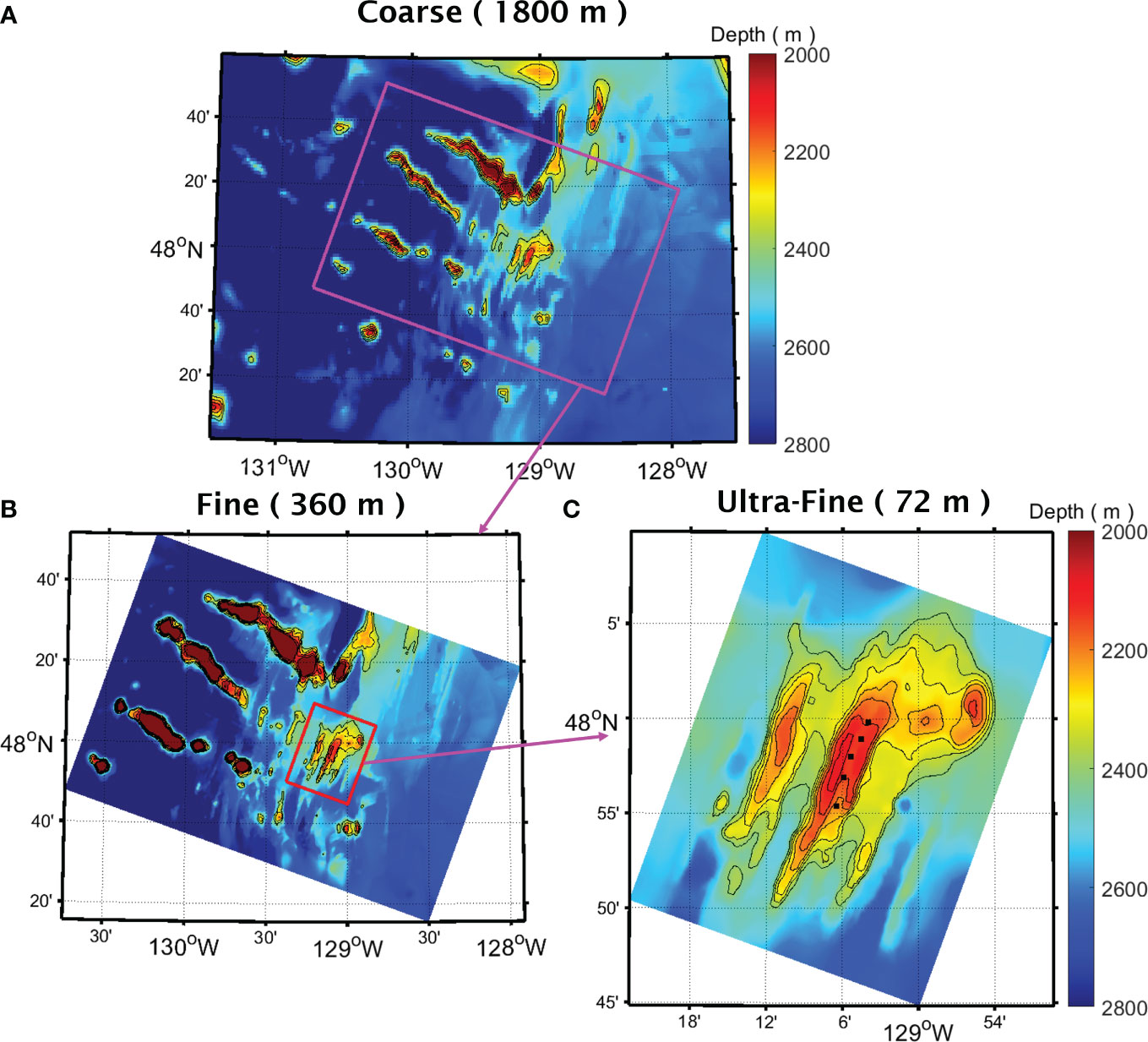
Figure 2 (A) Bathymetry within the coarse domain of the intermediate simulation. The box outlines the lateral boundaries of the fine domain of the nested multiscale simulations. (B) Bathymetry within the fine domain. The box outlines the nesting interface between the fine and ultra-fine grids. (C) Bathymetry within the ultra-fine domain. The black dots mark the locations of the five major hydrothermal vent fields within the axial valley of the Endeavour Segment.

The pilot simulation serves as a transition between the global reanalysis and our regional simulations, maintaining a grid refinement factor (i.e., the ratio of spatial resolutions between two consecutive grids) of approximately five. To account for tidal forcing, which is absent in the global reanalysis and the pilot simulation, we have added tidal elevation and barotropic currents acquired from the TPXO global tidal solution (Egbert and Erofeeva, 2002) to the lateral boundary forcing for the fine domain. We derive the surface forcings for both fine and ultra-fine domains from the same ERA5 3-hourly dataset used in the pilot simulation. The initial model fields used for the pilot simulation are constructed from the CMEMS global reanalysis data. The initial fields for the nested simulations are interpolated from the pilot simulation output onto the fine and ultra-fine grids. The computational time increments are 150 sec, 30 sec, and 6 sec on the coarse (pilot), fine, and ultra-fine grids, respectively.

The seafloor topography in our model is constructed from the Global Multi-Resolution Topography (GMRT) Synthesis of the Marine Geoscience Data System (Ryan et al., 2009). The original GMRT bathymetry has a spatial resolution of 250 m. Before interpolating on our model grids, we first apply a spatial median filter to smooth out features with length scales smaller than twice the size of a computational cell (i.e., the smallest resolvable wavelength). To further enhance numerical stability, we then apply the smoothing techniques described in Sikirić et al. (2009) to reduce the maximum stiffness ratio (Shchepetkin and McWilliams, 2005).

3.2 Hydrothermal venting and model parameters

The model incorporates the buoyancy generated by hydrothermal venting as bottom heat flux originating from the five major vent fields located within the axial valley. Specifically, each of the vent fields is represented as a 216 m by 216 m (3 by 3 cells) heat source in the ultra-fine domain. The corresponding heat flux is obtained from ship-based hydrographic surveys conducted in September 2004 (Kellogg and McDuff, 2010; Kellogg, 2011) and are prescribed as follows: 135 MW for Mothra, 306 MW for MEF, 387 MW for HR, 67.5 MW for Salty Dawg, and 4.5 MW for Sasquatch. In the model, the sources are treated as having no explicit volume flux. Consequently, the hydrothermal discharge is represented as thermally driven plumes. This simplified treatment of the plume sources is reasonable, considering that hydrothermal plumes are typically characterized as ‘lazy’ plumes (Hunt and Kaye, 2005). In such cases, the volume flux of the source has negligible influence on the plume’s behaviour and dynamics downstream. The vertical eddy viscosity and diffusivity in the model are determined using the Mellor-Yamada 2.5 level turbulent closure scheme (Mellor and Yamada, 1982), which has been shown in previous studies to enable simulation of vertical motions of plume fluid and the associated entrainment of ambient seawater into the plume, despite the use of the hydrostatic approximation (Thomson et al., 2005; Thomson et al., 2009).

3.3 Simulation timeframe and settings

In this study, we have conducted simulations covering two calendar-year periods: 2016 and 2021. We selected these years primarily due to the availability of concurrent observational data, which can be used for model validation. Those observations include the time series of flow velocity measured by current meters on cabled moorings deployed within the axial valley of Endeavour as part of the NEPTUNE seafloor observatory infrastructure by Ocean Networks Canada (Kelley et al., 2012) (Figure 1B). Additionally, comparing the model outputs between these two one-year periods enables us to investigate the interannual variability in ocean circulation and plume dispersion near the ridge segment.

To investigate how ocean tides and buoyancy from seafloor venting impact plume dispersion and ocean circulation near the ridge segment, we have conducted three runs for the 2016 simulation. The primary simulation output for model validation and interpretation was obtained from the first run, referred to as ‘baseline’ hereafter, which utilized the full set of forcings described in Sections 3.1 and 3.2. The remaining two runs employed a similar model configuration, but with a reduced set of forcings. Specifically, the second run, referred to as ‘no tide’ hereafter, included buoyancy from venting but not ocean tides, while the third run, referred to as ‘no vent’, included ocean tides but not buoyancy from venting. Additionally, we have conducted one run of the 2021 simulation using the full set of forcings (2021 baseline).

4 Model-observation comparison

4.1 Flow velocity time series

Our evaluation of the accuracy of simulated flow velocities utilizes concurrent, collocated comparisons with measurements obtained from the three current-meter moorings (RCM-NE, RCM-SE, RCM-SW) deployed within the axial valley of the Endeavour Segment (Figure 1B). Specifically, we utilized the current-meter time series from all three moorings to assess model skill during the 2016 simulation period. On the other hand, for the 2021 simulation period, we only used data from the two southern moorings (RCM-SW and RCM-SE) since no data was available from RCM-NE for most of the simulation period. We quantify the statistical agreement between the model and the observations using the Willmott Skill Score ($WSS$), which measures the normalized mean squared error in the forms of

$\begin{array}{ll}WS{S}_U=1-\frac{{\left|U_m-U_d\right|}^2}{{(\left|U_m-U_m\right|+\left|U_d-U_d\right|)}^2}& (1)\end{array}$

and

$\begin{array}{ll}WS{S}_V=1-\frac{{\left|V_m-V_d\right|}^2}{{(\left|V_m-V_m\right|+\left|V_d-V_d\right|)}^2}& (2)\end{array}$

for the zonal ($U$) and meridional ($V$) flow velocities, respectively. In equations (1) and (2), the subscript ‘m’ denotes model output, while ‘d’ indicates observed data. The angled brackets (e.g., ${\left|U_m-U_d\right|}^2$) represent time averaging of the quantity enclosed within the brackets. The score is a measure of the similarity between the model output and the observed data. The score ranges from 0 to 1, with higher values indicating better model performance (Willmott, 1981). The $WSS$ listed in Table 1 suggest that the model performs better at simulating the meridional velocity ($V$) than the zonal velocity ($U$).

TABLE 1

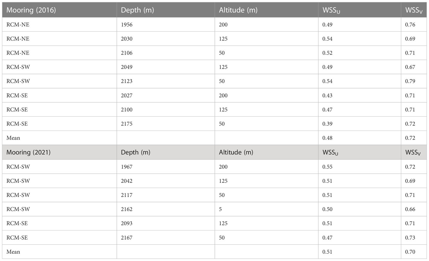
Table 1 Willmott Skill Scores ($WSS$) calculated from the measured and simulated flow velocity during July – Oct 2016 and Jul – Dec 2021.

A one-to-one comparison between the simulated flow velocities and measurements for all three moorings demonstrates an encouraging level of agreement. Considering flow at RCM-SW in 2021 for illustration (Figure 3), the observed currents predominantly flow in directions that are roughly aligned with the orientation of the ridge-axis at RCM-SW. This alignment is likely caused by the steering of flow within the topographic confinement of the axial rift valley. At a depth of 2162 m, just 1 m above the seafloor (Figure 3G), the direction of the observed currents oscillated between south-southwest (SSW) and north-northeast (NNE). This included an episode of intensified southwestward flow around Oct 27th, 2021. During that episode, the magnitude of the 2-day averaged flow velocity reached a maximum of 7.4 cm/s, compared with a median magnitude of 0.8 cm/s over the measurement period. At a shallower level, at 2117 m depth (Figure 3E), the direction of the observed currents was primarily SSW and only occasionally switched to north-northwest (NNW). Higher in the water column, at 2042 m and 1967 m depths which are shallower than the confining depths of the axial rift valley (Figure 3A, C), the westward component of the observed flow velocity was more prominent and the predominant flow direction was rotated toward the west-southwest (WSW), likely indicating a weakening of topographic steering effects at these higher altitudes. Encouragingly, the magnitude and direction of the simulated velocities (Figure 3B, D, F, H) are largely consistent with the observations at all depths at RCM-SW. There are two notable exceptions to this general case, 1) at 2042 m depth, the change of flow direction from SW to NW that occurred around Oct 16, 2021 is much less pronounced in the model velocity (Figure 3C vs 3D); 2) at 2162 m depth, the episode of intensified currents around Oct 27th, 2021 is absent in the simulated velocity (Figure 3G vs 3H).

FIGURE 3

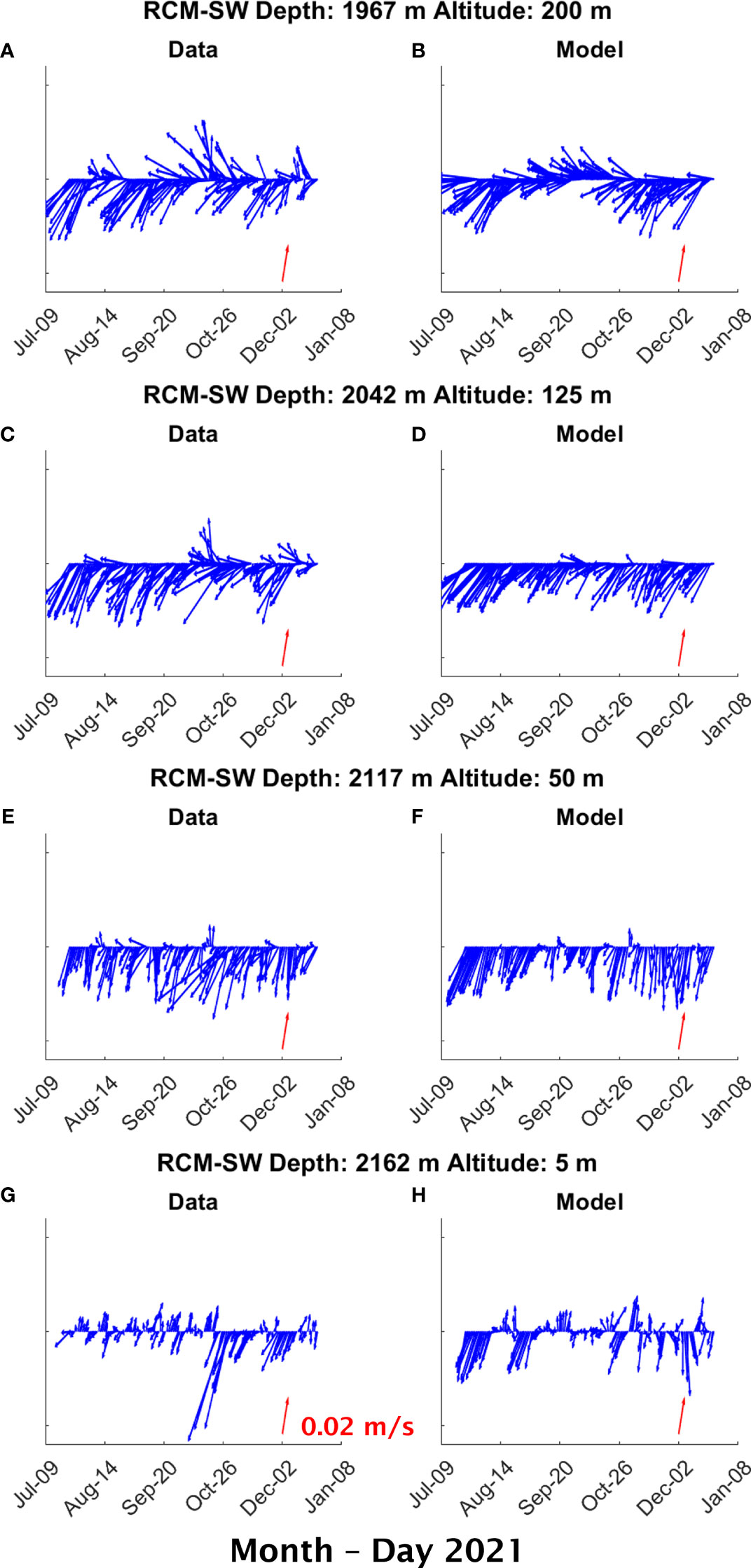
Figure 3 Comparison between measured (left) and simulated (right) 2-day averaged flow velocity at 1967 m (A, B), 2042 m (C, D), 2117 m (E, F), and 2162 m (G, H) depths at current-meter mooring RCM-SW during Jul – Dec 2021. The red arrow denotes velocity of 0.02 m/s with a heading of 20° relative to true north, which corresponds to the orientation of the ridge segment.

At mooring RCM-SE, (Supplementary Figure 1) the observed currents at 2093 m and 2167 m depths are not as well aligned with the ridge segment as they are at similar depths at RCM-SW, despite the proximity of the two moorings (Figure 1B, Supplementary Figure 1). In particular, the observed currents at 2167 m depth predominantly flow in the NNW direction (Supplementary Figure 1C), differing from the currents observed at approximately the same depth at RCM-SW that oscillated between SSW and NNE (Figure 3G). In comparison, at 2093 m depth, the observed flow direction at RCM-SE is primarily SSW, occasionally shifting to NNW (Supplementary Figure 1A). This vertically sheared flow structure between 2167 m and 2093 m depths at RCM-SE is not observed at RCM-SW. However, the simulated flow velocity for RCM-SE does faithfully reproduce a similar vertical sheared structure, with currents predominantly flowing in the NNW and SSW directions at 2167 m and 2093 m depths, respectively. One notable discrepancy between measured and simulated flows at the RCM-SE locale is that the simulated SSW flow at 2093 m depth is more uniformly consistent than the observations (Supplementary Figure 1a vs 1b). The differences in observed currents between RCM-SW and RCM-SE reveal evidence for a complex flow pattern that exhibits both horizontal and vertical shear along the ridge segment, especially within the axial valley. Overall, these features are reproduced, at least qualitatively, by the model.

For the 2016 simulation period, the flow velocities obtained from the simulation generally match the measurements taken at the RCM-NE (Supplementary Figure 2), RCM-SE (Supplementary Figure 3), and RCM-SW (Supplementary Figure 4) moorings. However, one notable distinction is evident for the current meter situated at a depth of 1956 m on RCM-NE, where the observed currents (Supplementary Figure 2A) predominantly flow southward throughout most of the simulation period. In comparison, the simulated flow velocity (Supplementary Figure 2B) primarily exhibits a westward direction, transitioning from NNW to SSW during the initial few months of the simulation period, and subsequently shifting towards a southward direction for the remainder of the simulation period. At the RCM-SE mooring for the same period, both the observed and simulated currents at 2027m predominantly flow southward, but the observed flow velocity exhibits a larger magnitude compared to the simulated flow velocity, which also has a stronger westward component (Supplementary Figure 3A,B).

4.2 Flow velocity spectrum

To assess the model’s proficiency in reproducing the oscillations in flow velocity at various frequencies, we have computed the power spectra for both observed and simulated velocity time series at RCM-SW (Figure 4) for the 2021 simulation period and at RMC-NE (Supplementary Figure 5) for the 2016 simulation period. The spectrum of the measured flow velocity exhibits prominent peaks at semi-diurnal (S, ~2 cycles/day) and diurnal (D, ~1 cycle/day) tidal frequencies, as well as near the local inertial frequency (f, ~1.48 cycles/day) at the mooring sites. Moreover, the flow velocity measured at all but the lowest current meter (5 m above bottom) on RCM-SW in 2021 (Figure 4) displays significant oscillations in the observational data within the ‘weather’ band previously noted, with a peak near a period of 4 days in the clockwise component of the spectrum (Cannon and Thomson, 1996; Thomson et al., 2003).

FIGURE 4

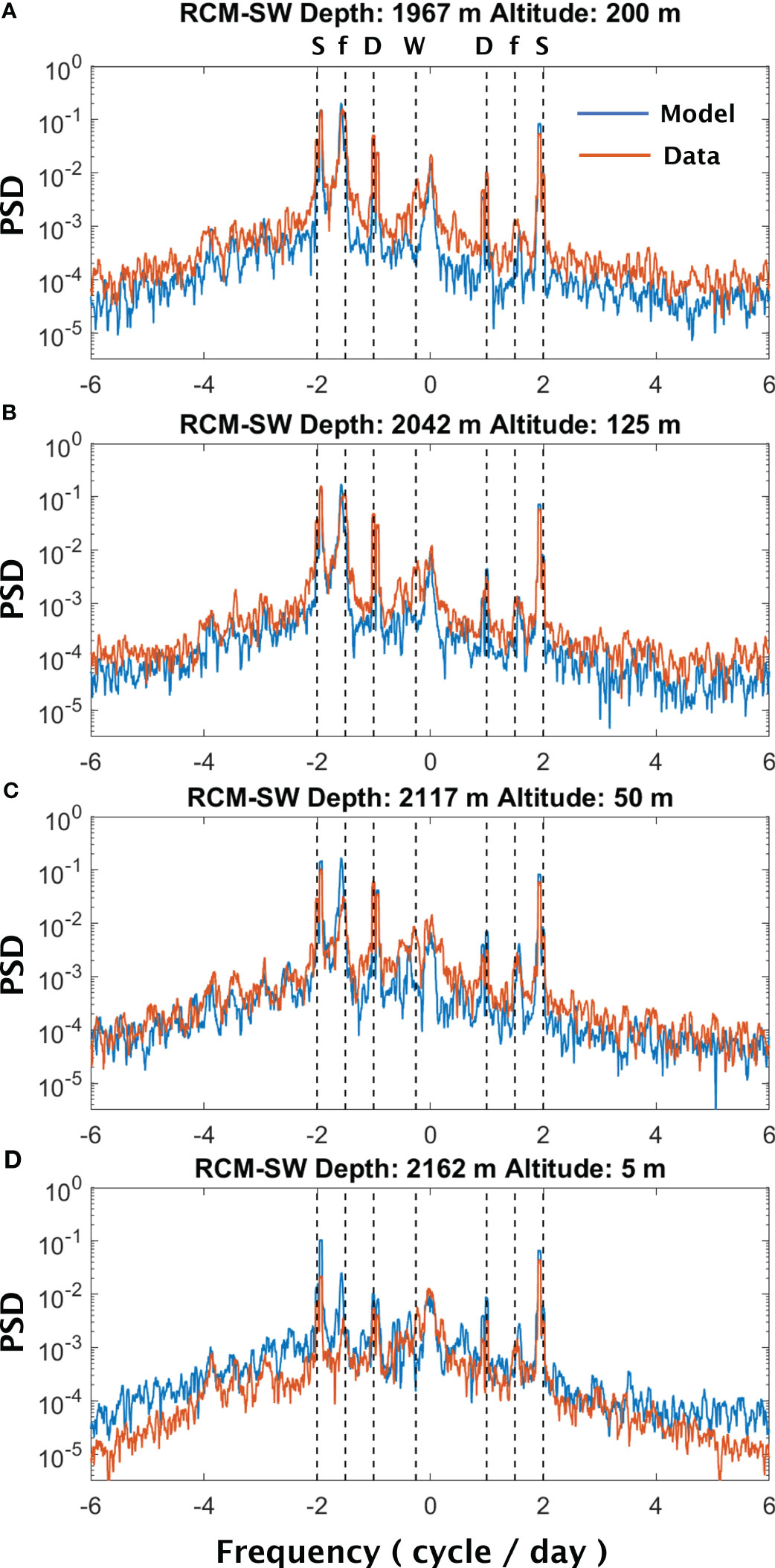
Figure 4 Power spectral density (PSD) computed from the measured (red) and simulated (blue) 4-hr averaged flow velocity at 1967 m (A), 2042 m (B), 2117 m (C), and 2162 m (D) depths at current-meter mooring RCM-SW during Jul – Dec 2021. The negative frequencies correspond to the clockwise (CW) rotatory component of the spectrum, while the positive frequencies correspond to the counterclockwise (CCW) rotary components of the spectrum. The vertical dashed lines denote spectral peaks corresponding to the semi-diurnal tidal (S) (~2 cycle/day), inertial (f) (~1.48 cycle/day), diurnal tidal (D) (~1 cycle/day), and the 4-day ‘weather’ band (W) (~0.25 cycle/day) oscillations.

In comparison, the spectra derived from simulated flow velocity time series demonstrate overall agreement with the observations, with a few noticeable discrepancies. Firstly, the simulated flow velocity lacks the 4-day ‘weather’ band oscillations present in the observations. Secondly, the model appears to overestimate the near-inertial oscillations (f) at the current meters located close to the seafloor, specifically at altitudes of 50 m and 5 m (Figures 4C, D and Supplementary Figure 5C). As indicated by Thomson et al. (2003), the near-inertial oscillations experience significant attenuation within the rift valley of the Endeavour Segment. This previous finding is consistent with our current observations, which demonstrate a decrease in the magnitude of the near-inertial spectral peak as depth increases (Figure 4 and Supplementary Figure 5). On the other hand, the simulated flow velocity shows less prominent attenuation of near-inertial oscillations within the axial valley. This discrepancy can likely be attributed to the smoothing of the bathymetry used in the simulations, which is done to enhance computational stability and reduce numerical errors. The bathymetric smoothing process within the model potentially suppresses the ruggedness of the axial valley, thus reducing its damping effect on near-inertial oscillations. The reason behind the absence of 4-day oscillations in simulated flow velocity remains unclear. Cannon and Thomson (1996) attributed the occurrence of these oscillations observed along the Juan de Fuca Ridge to local storms. Therefore, the lack of such oscillations in our simulations may indicate an inadequate representation of local storm events in the surface forcing used by the model (Section 3.1).

4.3 Plume distribution

To evaluate the model skill in simulating plume dispersion, we compare the characteristics of the non-buoyant cap of the plume generated by the model with observations from previous studies (Baker and Massoth, 1987; Thomson et al., 1992; Kellogg and McDuff, 2010). Specifically, we focus on three key properties of the plume’s non-buoyant cap: height, core potential temperature anomaly, and core density. Our analysis shows that in the two instances demonstrated in Figures 5, 6, the buoyant plumes rising from the five major vent fields coalesce and reach neutral buoyancy at a height of 100 – 200 m above the floor of the axial valley. In the interior of the ultra-fine domain, within tens of kilometers of the ridge segment (Figures 5B, 6B), the non-buoyant plume cap disperses as a cohesive band in the NW and SW direction on Oct 2, 2016 and Aug 16, 2021, respectively. In comparison, as the plume cap spreads farther away from the ridge segment, it becomes more diffuse and displays meandering patterns (Figures 5A, 6A). In both cases, the core of the plume’s non-buoyant cap is situated at depths between 2000 m and 2050 m, between the 27.7 and 27.71 $kg/m^3$ isopycnic surfaces (Figures 5C, 6C). We calculate the isohaline potential temperature anomaly ($\text{Δ}{\theta }_S$) using the method described in Kellogg and McDuff (2010) as the deviation of absolute potential temperature ($\theta$) from a reference for a given salinity ($S$). To obtain the reference temperature, we fit a second-order polynomial to the model $\theta$/$S$ data between 1700 m and 2300 m depths at three background stations (Figures 5B, 6B). These stations are located east of the MEF at (47.95°N, 128.94°W), (47.95°N, 128.85°W), and (47.95°N, 128.81°W), respectively. The resulting $\text{Δ}{\theta }_S$ at the core of the non-buoyant plume exhibited a maximum, at a depth of 2050 m, of approximately 0.08°C and 0.10°C on Oct 2, 2016 and Aug 16, 2021, respectively (Figures 5D, 6D). In comparison, a hydrographic survey conducted along the axial valley in June 2004 showed hydrothermally influenced water with $\text{Δ}{\theta }_S\approx$ 0.10°C at the same depth (Kellog and McDuff, 2010).

FIGURE 5

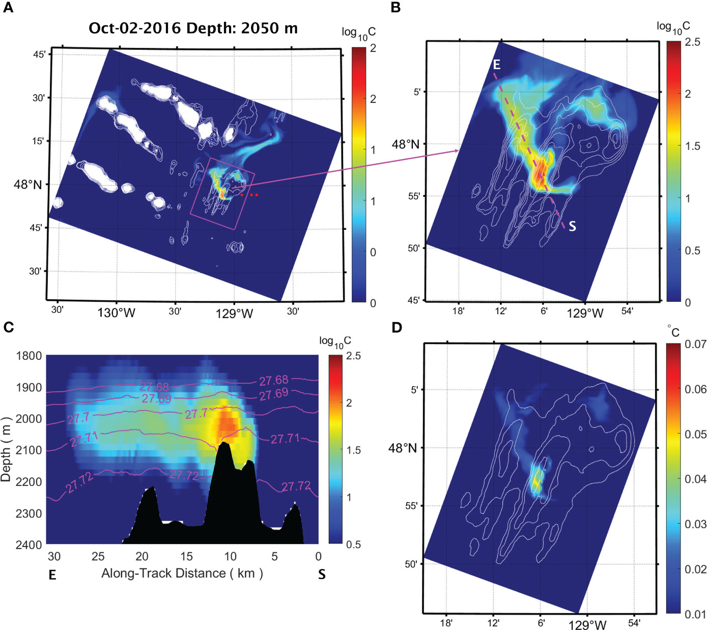
Figure 5 Concentration of a passive tracer released from the vent sources within the axial valley of the Endeavour Segment on Oct 2nd, 2016, shown in horizontal cross-sections across the interiors of the fine (A) and the ultra-fine (B) domains at 2050 m depth. The red dots in (A) mark the locations of the three background hydrographic stations. (C) a cross-section of the same tracer concentrations as in (B) along the transect indicated from start (S) to end (E). Contours denote isopycnic surfaces. (D) A horizontal cross-section of potential temperature anomaly at 2050 m depth within the same ultra-fine domain and as tracer concentration plot shown at (B).

FIGURE 6

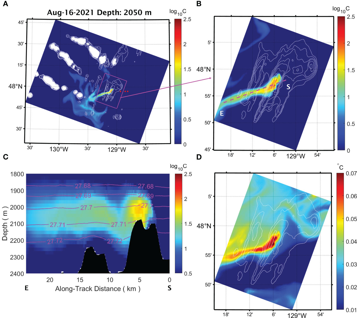
Figure 6 Concentration of a passive tracer released from the vent sources within the axial valley of the Endeavour Segment on Aug 16th, 2021, shown in horizontal cross-sections across the interiors of the fine (A) and the ultra-fine (B) domains at 2050 m depth. The red dots in (A) mark the locations of the three background hydrographic stations. (C) a vertical cross-section of the same tracer concentrations as in (B) along the transect indicated from start (S) to end (E). Contours denote isopycnic surfaces. (D) A horizontal cross-section of potential temperature anomaly at 2050 m depth within the same ultra-fine domain and as tracer concentration plot shown at (B).

5 Results and discussion

5.1 Near-ridge ocean circulation

The analysis of the 2016 baseline solution (Figure 7A) shows that the flow field, when averaged over a five-month period from July to November 2016, exhibits an anti-cyclonic circulation (clockwise in the northern hemisphere) that is centered around the high point on the western side of the ridge segment. Specifically, there is a poleward along-ridge flow over the western flank of the ridge, while an equatorward along-ridge flow is present over the eastern flank (Figure 8A). At the core of these ridge flank jets, the velocity reaches a maximum of approximately 0.04 m/s at a depth about 2050 m. A similar anti-cyclonic circulation has been observed around the North Cleft Segment of the southern JDFR and was attributed to two potential generation mechanisms: hydrothermal forcing and tidal rectification (Cannon and Pashinski, 1997). More specially, the entrainment of ambient seawater into buoyant hydrothermal discharge can drive an anti-cyclonic circulation at the spreading level of the non-buoyant plume cap (Speer, 1989). Additionally, tidal rectification has been shown to generate anti-cyclonic residual currents around pronounced topographic features such as Georges Bank (Chen and Beardsley, 1995) and Axial Seamount (Xu and Lavelle, 2017).

FIGURE 7

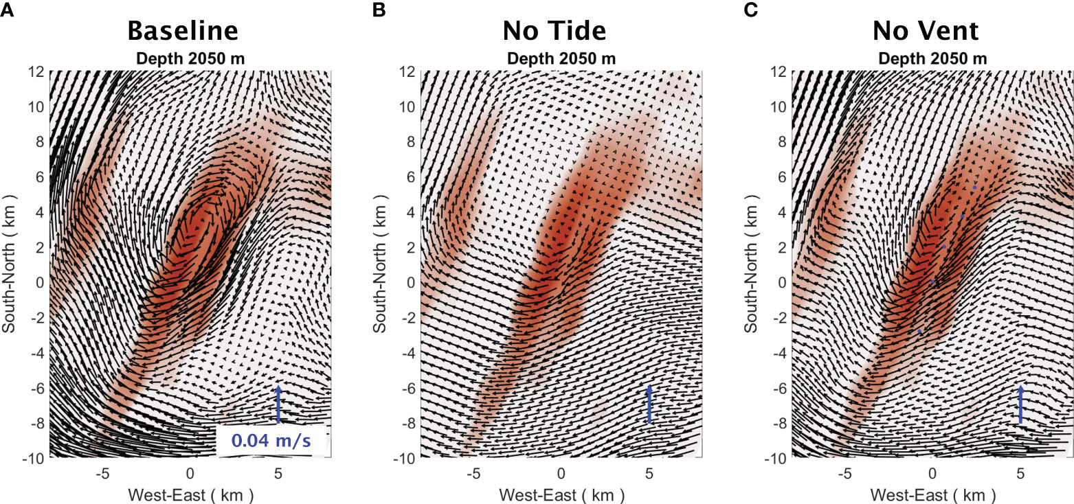
Figure 7 Flow velocity averaged over a five-month period from Jul 1st to Nov 30th, 2016, at 2050 m from (A) the baseline solution of the 2016 simulation, (B) the no-tide run, and (C) the no-vent run. The blue arrow denotes a northward flow of 0.04 m/s.

FIGURE 8

Figure 8 Velocity sections in the along-ridge (A–C) and cross-ridge directions (D–F) averaged over a 5-month period, from Jul 1st to Nov 30th, 2016, plotted in vertical cross-sections along a 10 km long transect that runs perpendicular to the ridge axis and passes through HR at the center of the transect. The panels in the left column (A, D) show the results of the baseline solution of the 2016 simulation, while the panels in the middle (B, E) and right (C, F) columns display the results of the no-tide and no-vent runs, respectively. A positive along-ridge velocity is oriented 20 from true north, and a positive cross-ridge velocity is oriented 110 from true north.

A comparison between the baseline solution and the results of the no-tide run indicates that the anti-cyclonically sheared mean flow across the ridge segment substantially weakens after the removal of the tidal forcing (Figure 7A vs 7B, Figure 8A vs 8B). Furthermore, a comparison between the baseline solution and the results of the no-vent run also shows a reduction in the strength of the anti-cyclonic flank jets along the ridge-axis, albeit to a lesser extent (Figure 7A vs 7C, Figure 8A vs 8C). Taken together, these comparisons suggest that tidal forcing is likely the primary driver of the anti-cyclonic circulation around the ridge segment, with hydrothermal venting playing a secondary role. This finding is consistent with Cannon and Pashinski (1997)’s conclusion that tidal forcing is the dominant generation mechanism for the anti-cyclonic circulation around the North Cleft Segment.

The buoyant hydrothermal plumes that rise from the axial valley draw in surrounding water and drive an inflow, which is most pronounced around the HR vent field with which exhibit the highest heat outputs (Figures 9A, C). This inflow alters the near-bottom mean flow within the axial valley, which is primarily directed along the ridge axis in the SSW direction in the absence of venting (Figure 9B). In comparison, the venting-induced local circulation causes the mean flow to become cyclonically sheared within the valley, with an equatorward current on the western side and poleward current on the eastern side (Figures 8A, 9A, B). This cyclonically sheared flow pattern is also evident in current-meter measurements from the RCM-SW and RCM-SE moorings in 2016. At approximately 50 m above the seafloor, the current at RCM-SW on the western side of the valley primarily flowed in an equatorward direction along the ridge axis, while the current measured at RCM-SE on the eastern side of the valley was primarily poleward along the ridge axis (Supplementary Figure 3E vs Supplementary Figure 4C). The model currents sampled at the same locations as these two moorings show reasonable agreement with the measurements (Supplementary Figures 3, 4). Previously, current velocity measurements within the axial valley had been interpreted in such a way as to suggest that venting drives a steady near-bottom flow into the valley from its northern and southern ends (Thomson et al., 2003). However, the long-term current-meter measurements and concurrent simulation results presented here reveal a more complex venting-induced flow structure that is cyclonically sheared across the valley. Our findings are consistent with those from a previous numerical study, which showed a similar cyclonically sheared near-bottom flow within the axial valley, using realistic ridge topography, a near-steady cross-ridge flow and hydrothermal venting as forcing (Thomson et al., 2009). Based on previous laboratory and numerical studies (e.g., Speer, 1989; Helfrich and Battisti, 1991; Speer and Marshall, 1995; Fabregat Tomàs et al., 2016), it has been observed that the influx of surrounding water into a turbulent buoyant plume drives a local circulation that is anti-cyclonic near the spreading level of the non-buoyant plume cap and cyclonic around the plume stem below. In our simulations that account for realistic ridge topography, the deeper forced circulation, driven by the convergent flow towards the plume within the confinement of the axial valley, leads to the formation of the cyclonically sheared mean flow within the valley (Figures 8A, 9A, C). Meanwhile, the divergent flow out of the non-buoyant plume cap contributes to the formation of the anti-cyclonically sheared mean flow at depths overlying the axial valley floor (Figure 7A).

FIGURE 9

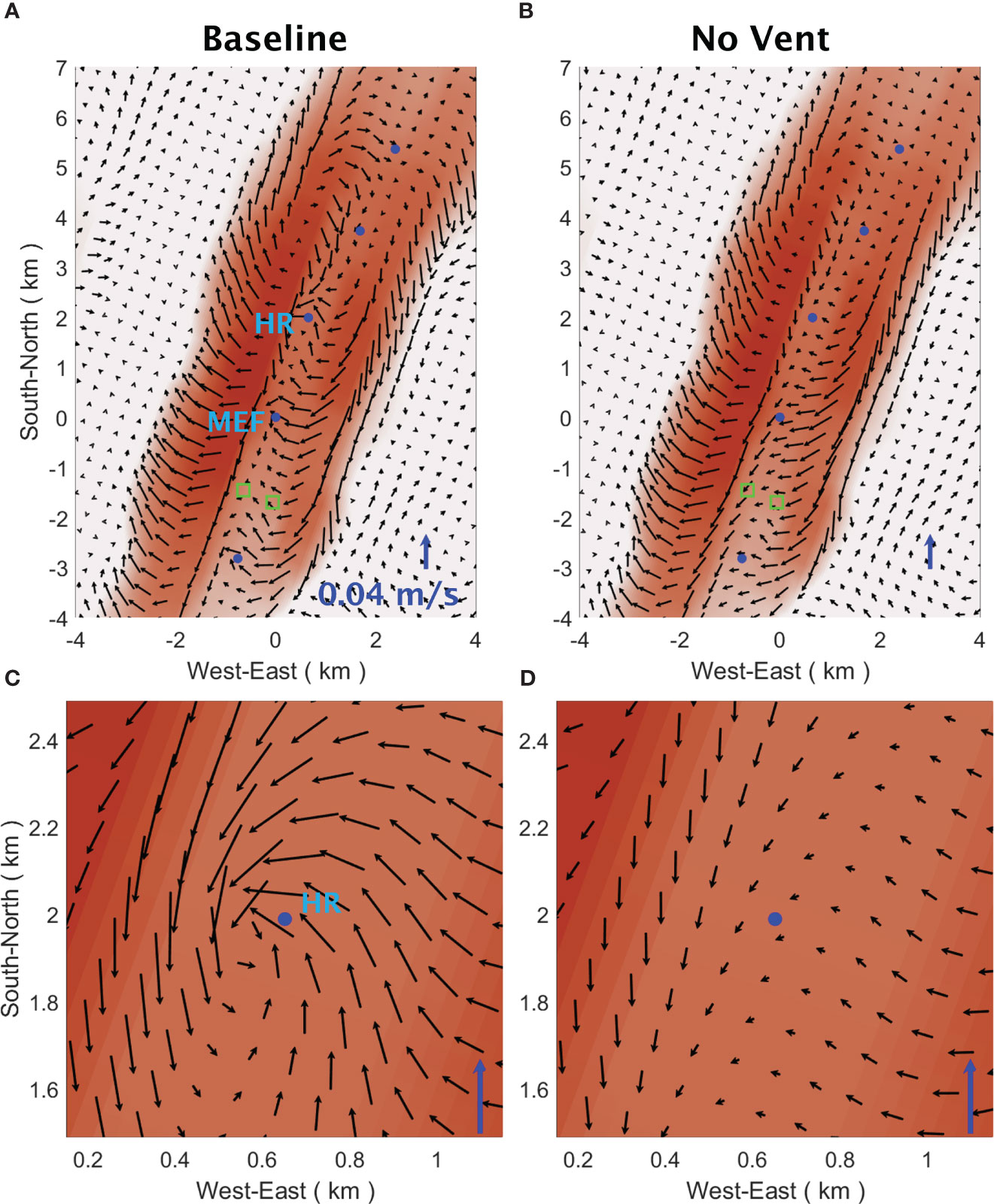
Figure 9 Near bottom flow velocity within the axial valley and surrounding areas, averaged over a five-month period (Jul 1st to Nov 30th, 2016). The velocity data is taken from the second terrain-following layer above the seafloor. (A) shows the results of the baseline solution of the 2016 simulation, while (B) depicts the results of the no-vent run. The blue dots mark the locations of the five major hydrothermal vent fields within the axial valley. The green squares denote the locations of the current-meter moorings RCM-SW (on the western side of the valley) and RCM-SE (on the eastern side of the valley). (C, D) show the flow velocity within the immediate vicinity of the High Rise (HR) vent field. The blue arrow in each panel denotes a northward flow of 0.04 m/s.

5.2 Dispersion of hydrothermal plumes

The 2016 baseline solution shows that, within the ultra-fine domain, the non-buoyant plume cap disperses primarily towards the north within a few tens of kilometres from the Endeavour Segment (Figures 10A, C, E). As the plume travels further away (Figures 11A, C, E), it splits into two branches near the Endeavour Seamount (ESM) and the southern end of the West Valley Segment (WVS) of the JDFR, which lies immediately to the north of the Endeavour Segment. One of those branches continues its northward movement, to the east of Endeavour Segment, while the other turns westward flowing south of the Heck Seamount chain (Figures 11A, C, E). In comparison, the no-tide run shows a similar northward dispersion within the vicinity of the Endeavour Segment (Figures 10B, D, F). Farther afield, however, instead of bifurcating into northward and westward moving branches as in the baseline solution, the plume veers to the northeast past Endeavour Seamount (Figures 11B, D, F). This disparity in plume dispersion patterns can be attributed to the existence of tidally rectified anti-cyclonic circulation in the baseline solution around Endeavour Seamount, the West Valley Segment, and the Heck Seamount (HSM) chain (Supplementary Figure 6A). In particular, the baseline solution shows a strong northwestward current flowing along the south-facing flanks of these topographic structures, which drives the westward moving branch of the plume fluid. This current is significantly weaker in the no-tide run, explaining the observed deviation in plume dispersion (Supplementary Figure 6B).

FIGURE 10

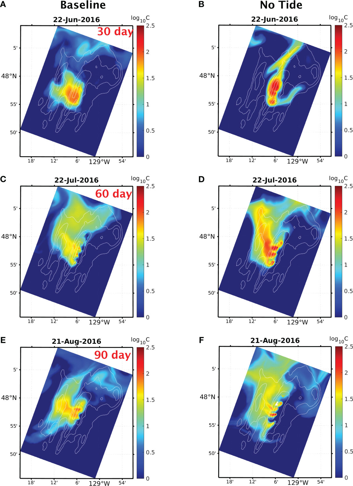
Figure 10 Comparison of the dispersion of a passive tracer released from the vent sources within the axial valley of the Endeavour Segment across the interior of the ultra-fine domain from the baseline solution (left column) and the no-tide run of the 2016 simulation. The tracer concentration is plotted across the interior of the fine domain on: (A, B) Jun 22nd (30 days after the onset of venting), (C, D) Jul 22nd (60 days after), and (E, F) Aug 21st (90 days after). The colorbar indicates the range of maximum tracer concentration between 26.69 $kg/m^3$ and 27.71 $kg/m^3$ isopycnal surfaces on a logarithmic scale.

FIGURE 11

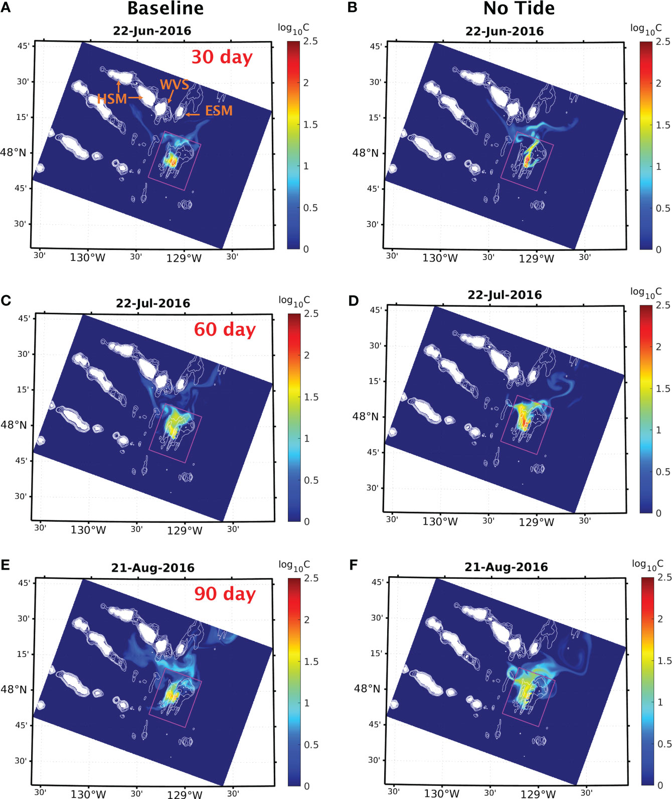
Figure 11 Comparison of the dispersion of a passive tracer released from the vent sources within the axial valley of the Endeavour Segment across the interior of the fine domain from the baseline solution (left column) and the no-tide run of the 2016 simulation. The tracer concentration is plotted across the interior of the fine domain on: (A, B) Jun 22nd (30 days after the onset of venting), (C, D) Jul 22nd (60 days after), and (E, F) Aug 21st (90 days after). The colorbar indicates the range of maximum tracer concentration between 26.69 kg/m3 and 27.71 kg/m3 isopycnal surfaces on a logarithmic scale. The box outlines the boundaries of the ultra-fine domain. The arrows in (A) mark the locations of Endeavour Seamount (ESM), the West Valley Segment (WVS), and the Heck Seamount chain (HSM).

To investigate the interannual variability of plume dispersion patterns, we have calculated the plume occupancy rates for both the 2016 baseline and 2021 baseline simulation results. These rates represent the proportion of time that a given location is occupied by a hydrothermal anomaly at the depth of the non-buoyant plume cap (Figure 12). The results reveal a shift in dispersion direction between 2016 and 2021. Specifically, the 2016 simulation results show that the non-buoyant plume cap primarily dispersed towards the north of the Endeavour Segment before splitting into two branches that continued northward and westward, respectively. In contrast, the 2021 simulation results demonstrate that the plume cap primarily dispersed towards the southwest of the Endeavour Segment then southward farther away from the ridge segment. This southwest dispersal direction is more consistent with previous field observations of the non-buoyant plume cap by Baker and Massoth (1987). Meanwhile, the north-to-south change of dispersion direction between 2016 and 2021 suggests that the trajectory of the plume can vary significantly on interannual time scales.

FIGURE 12

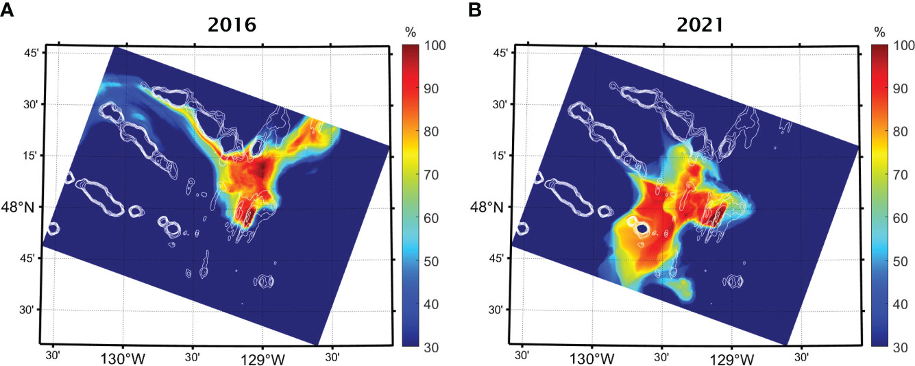
Figure 12 Plume occupancy rates calculated from (A) the 2016 baseline solution and (B) the results of the 2021 simulation.

What might be the cause of such pronounced inter-annual variability? Large-scale abyssal flow plays a critical role in driving the dispersion of hydrothermal plumes, particularly in off-axis regions. Consequently, a plausible explanation for the change in dispersion direction between 2016 and 2021 could be a shift in the direction of abyssal flow near the depth of the non-buoyant plume cap, around 2100 m (Figures 5C, 6C). To investigate this proposed explanation, we have examined the flow field at a depth of 2100 m from the CMEMS global reanalysis (Fernandez and Lellouche, 2021) for July to September of 2016 and 2021, respectively (Figure 13). The results exhibit a noticeable alteration in the flow direction within the regions surrounding the Endeavour Segment. Specifically, in 2016, currents flowed northward across the ultra-fine domain (Figure 13A), whereas in 2021, the predominant flow was southwestward over and to the east of the ridge axis, and westward over the western flank (Figure 13B). These flow directions are largely consistent with the plume dispersion directions observed in our simulations for both 2016 and 2021.

FIGURE 13

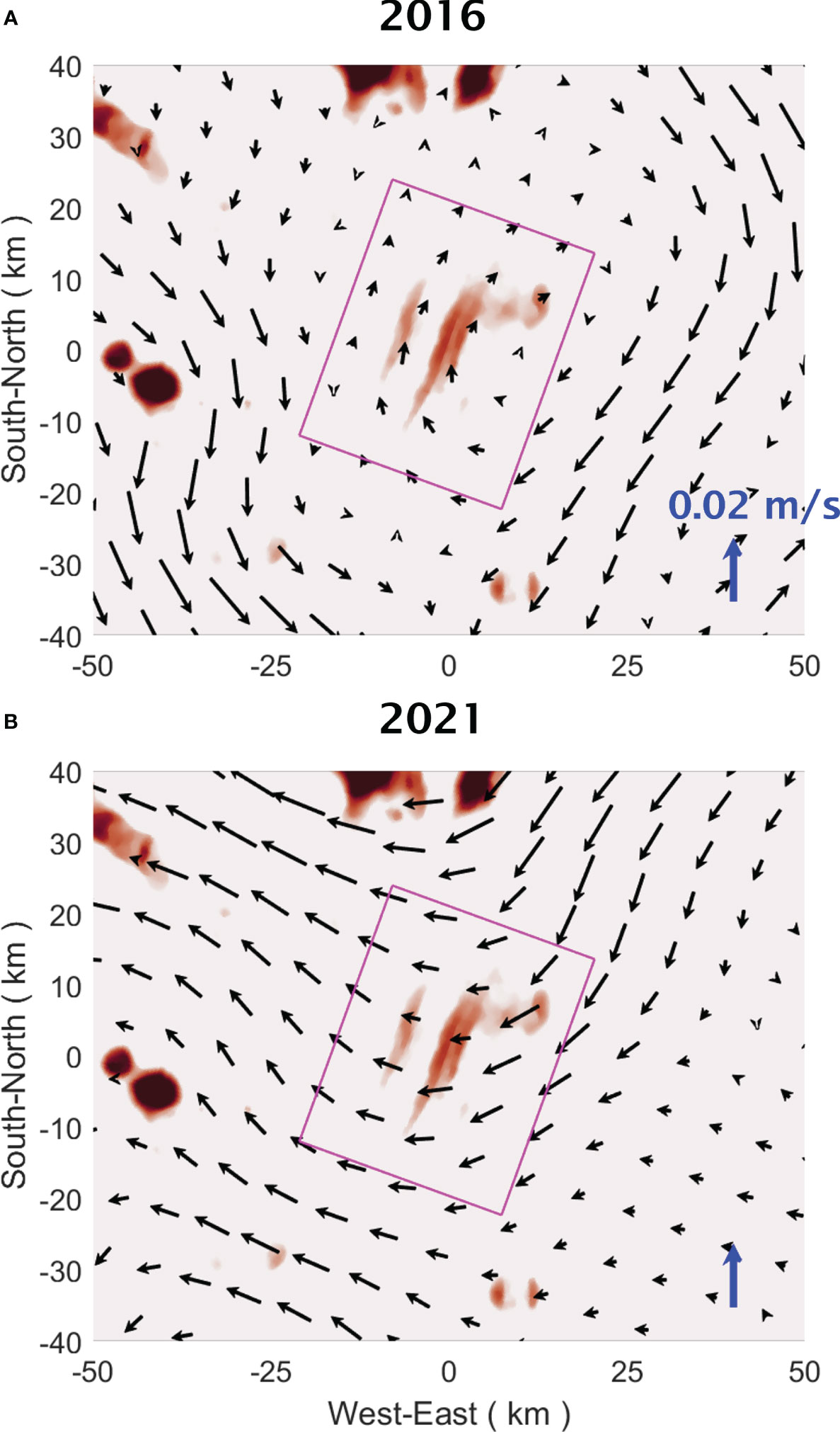
Figure 13 Flow velocity at 2100 m depth from the CMEMS global reanalysis averaged over a three-month period of July to September in 2016 (A) and 2021 (B).

5.3 Mixing of hydrothermal plumes

The hydrothermal anomaly, which is quantified by the concentration of the passive tracer released from the source vent sites, exhibits higher values in the non-buoyant plume cap in our no-tide simulation results when compared to the baseline solution results (Figures 10, 11). Generally, a larger hydrothermal anomaly indicates a lower degree of plume fluid dilution and thus less entrainment of ambient seawater. Previous laboratory and numerical studies have demonstrated that the presence of a cross-flow enhances the entrainment of ambient water into a buoyancy-driven plume, yielding increased dilution factors (e.g., Xu and Di Iorio, 2012). To quantify the mixing of plume fluid with ambient seawater, we calculate the volume integrated variance of the concentration of the passive tracer ($C)$ released from the source vents as

$\begin{array}{ll}Var(C)={\displaystyle \underset{V}{\int }{C}^{\prime 2}dV}& (3)\end{array}$

In equation (3), $C^{\prime }=C-C_m$, $C_m$ being the tracer concentration averaged over the integration volume ($V$), which encloses the interior of the final domain, bounded by the seafloor and the sea-surface. The loss of variance of a conservative tracer is a well-established approach for defining mixing in studies of ocean turbulence (e.g., Burchard and Rennau, 2008; Wang and Geyer, 2018). More recently, destruction of salinity variance has been used to quantify mixing in estuaries (e.g., MacCready et al., 2018; Broatch and MacCready, 2022).

In our simulations, during the time between when the tracer is released and when it reaches the lateral boundaries of the integration volume, tracer variance is produced at the source vents on the seafloor and destroyed within the volume of the plume due to mixing of plume fluid with ambient seawater. A comparison among the four simulation runs demonstrates that: $Var(C)$ computed from the 2016 no-vent simulation results has the highest overall value over a 70-day period starting from the onset of tracer release; $Var(C)$ computed from the 2016 no-tide run has the second highest overall value; $Var(C)$ computed from the 2016 baseline solution and the 2021 baseline solution have the lowest overall values (Figure 14). This suggests that the buoyancy flux from venting and tidal forcing both enhance mixing of hydrothermal plumes with ambient seawater, but that the buoyancy flux effect has the larger impact.

FIGURE 14

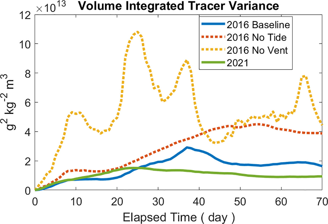
Figure 14 Volume integrated tracer variance over a 70-day period following when the tracer is released from the 2016 baseline solution (solid blue), no-tide run (dotted red), no-vent run (dotted yellow), and the 2021 simulation results (solid green).

5.4 Limitations and future research implications

The preceding simulation results demonstrate the model’s proficiency in capturing the dispersion of hydrothermal plumes within a complex flow field that arises from the dynamic interaction between abyssal flow, ocean tides, and the topography of the ridge segment. Nonetheless, the comparison of the simulated flow velocity with direct measurements has revealed certain discrepancies, which may affect the accuracy of simulated plume distributions and trajectories with implications for future research efforts. The most apparent discrepancy is the absence of the 4-day ‘weather’ band oscillations in the simulated flow velocity (Figure 4). Previous observations by Cannon and Thomson (1996) have indicated that these oscillations could have a significant impact on the dispersion of hydrothermal plumes near the ridge axis. Therefore, the absence or misrepresentation of these oscillations in our simulations has the potential to undermine their overall accuracy, particularly concerning the dispersion of hydrothermal plumes in close proximity to the ridge segment.

As mentioned in Section 4.2, the lack of 4-day oscillations in the simulated flow velocity could potentially be attributed to inaccuracies in the surface atmospheric forcing, such as wind stress, employed in the model. While a definitive understanding of the generation mechanism for the 4-day oscillations remains elusive, previous studies have indicated that these oscillations are associated with local storms (Cannon et al., 1991; Cannon and Thomson, 1996) and could be characterized as ridge-trapped subinertial waves (Allen and Thomson, 1993). In order to gain further insights into the generation of the 4-day oscillations along the Endeavour Segment and other regions of the JDFR, a potentially effective approach would involve diagnosing the factors contributing to the absence of these oscillations in our simulations. By making adjustments to the surface forcing and other model parameters, we can strive for an improved representation of these oscillations in future numerical studies. This approach holds promise for enhancing our understanding of the mechanisms underlying the 4-day oscillations and their behavior along the JDFR, making an important avenue for future research.

Additionally, we can achieve a more robust and comprehensive validation of our modeling framework by leveraging the continuously advancing capabilities of deep-diving autonomous underwater vehicles (AUVs). A carefully designed field program, employing an AUV equipped with dedicated in-situ instruments, would be able to provide direct observations of plume-specific tracers across a wide spatial area. Such future AUV-based plume surveys would be able to complement the use of the data collected by stationary instruments, such as the current-meter mooring data employed here, enhancing our assessment of model performance by enabling us to compare simulated plume distributions and trajectories with field observations.

6 Summary

The multiscale simulations conducted in this study have yielded valuable insights into flow dynamics and hydrothermal plume dispersion near the Endeavour Segment of the JDFR:

● The time-averaged flow field exhibits an anti-cyclonic circulation around the ridge segment, with a northward flow over the western side of the ridge and a southward flow over the eastern side. Tidal forcing is identified as the primary driver of this anti-cyclonic circulation, while hydrothermal venting is a secondary contributing mechanism. Within the axial rift valley, hydrothermal venting induces cyclonic circulation around vent sites through entrainment by buoyant plumes. This cyclonic circulation is most evident around High Rise, which has the highest heat flux among the five major vent fields in the axial valley.

● Tidal forcing has a significant impact on plume dispersion, particularly near the large topographic features to the north of the Endeavour Segment.

● A comparison between the 2016 and 2021 baseline solutions has revealed significant inter-annual variability in hydrothermal plume dispersion, with the plume dispersing primarily north of the Endeavour Segment in 2016 and to the south of the segment in 2021.

● Both hydrothermal buoyancy flux and tidal forcing enhance the mixing of hydrothermal plumes with ambient seawater, with the buoyancy flux effect having a larger impact.

● In addition to elucidating the physical dispersion of heat and tracers away from the Juan de Fuca Ridge ridge-axis, we anticipate that this study may also prove valuable for informing future studies of biogeochemical processes that may be active within Endeavour segment hydrothermal plumes.

We have also identified two important avenues for future research:

● Investigating methods to enhance the performance of the model, with a specific focus on the accurate representation of the 4-day ‘weather’ band oscillations in flow velocity near the ridge segment.

● Exploring innovative approaches, such as the utilization of AUVs equipped with appropriate in situ sensors to augment field observations for comprehensive model validation.

Data availability statement

Publicly available datasets were analyzed in this study. This data can be found here: Ocean Networks Canada https://data.oceannetworks.ca/DataSearch.

Author contributions

This manuscript is the outcome of a collaborative effort between GX and CG, where GX took the lead in numerical modeling and data analysis, while CG contributed to data interpretation and presentation.

Funding

This study is funded by the National Science Foundation (award numbers: OCE-1851199 and OCE-1851007).

Acknowledgments

The authors would like to thank the NCAR Computational and Information System Lab (CISL) for providing the high-performance computing (HPC) platform and resources used for this work.

Conflict of interest

The authors declare that the research was conducted in the absence of any commercial or financial relationships that could be construed as a potential conflict of interest.

Publisher’s note

All claims expressed in this article are solely those of the authors and do not necessarily represent those of their affiliated organizations, or those of the publisher, the editors and the reviewers. Any product that may be evaluated in this article, or claim that may be made by its manufacturer, is not guaranteed or endorsed by the publisher.

Supplementary material

The Supplementary Material for this article can be found online at: https://www.frontiersin.org/articles/10.3389/fmars.2023.1213470/full#supplementary-material

References

Allen S. E., Thomson R. E. (1993). Bottom-trapped subinertial motions over midocean ridges in a stratified rotating fluid. J. Phys. oceanogr. 23 (3), 566–581. doi: 10.1175/1520-0485(1993)023<0566:BTSMOM>2.0.CO;2

CrossRef Full Text | Google Scholar

Baker E. T., Massoth G. J. (1987). Characteristics of hydrothermal plumes from two vent fields on the Juan de Fuca Ridge, northeast Pacific Ocean. Earth Planetary Sci. Lett. 85 (1-3), 59–73. doi: 10.1016/0012-821X(87)90021-5

CrossRef Full Text | Google Scholar

Berdeal I. G., Hautala S. L., Thomas L. N., Johnson H. P. (2006). Vertical structure of time-dependent currents in a mid-ocean ridge axial valley. Deep Sea Res. Part I: Oceanographic Res. Pap. 53 (2), 367–386. doi: 10.1016/j.dsr.2005.10.004

CrossRef Full Text | Google Scholar

Broatch E. M., MacCready P. (2022). Mixing in a salinity variance budget of the Salish Sea is controlled by river flow. J. Phys. Oceanogr. 52 (10), 2305–2323. doi: 10.1175/JPO-D-21-0227.1

CrossRef Full Text | Google Scholar

Burchard H., Rennau H. (2008). Comparative quantification of physically and numerically induced mixing in ocean models. Ocean Model. 20 (3), 293–311. doi: 10.1016/j.ocemod.2007.10.003

CrossRef Full Text | Google Scholar

Cannon G. A., Pashinski D. J. (1997). Variations in mean currents affecting hydrothermal plumes on the Juan de Fuca Ridge. J. Geophys. Res.: Oceans 102 (C11), 24965–24976. doi: 10.1029/97JC01910

CrossRef Full Text | Google Scholar

Cannon G. A., Pashinski D. J., Lemon M. R. (1991). Middepth flow near hydrothermal venting sites on the southern Juan de Fuca Ridge. J. Geophys. Res.: Oceans 96 (C7), 12815–12831. doi: 10.1029/91JC01023

CrossRef Full Text | Google Scholar

Cannon G. A., Thomson R. E. (1996). Characteristics of 4-day oscillations trapped by the Juan de Fuca Ridge. Geophys. Res. Lett. 23 (13), 1613–1616. doi: 10.1029/96GL01370

CrossRef Full Text | Google Scholar

Carbotte S. M., Canales J. P., Nedimović M. R., Carton H., Mutter J. C. (2012). Recent seismic studies at the East Pacific Rise 8 20'–10 10'N and Endeavour Segment: Insights into mid-ocean ridge hydrothermal and magmatic processes. Oceanography 25 (1), 100–112. doi: 10.5670/oceanog.2012.08

CrossRef Full Text | Google Scholar

Chen C., Beardsley R. C. (1995). A numerical study of stratified tidal rectification over finite-amplitude banks. Part I: Symmetric banks. J. Phys. Oceanogr. 25 (9), 2090–2110. doi: 10.1175/1520-0485(1995)025<2090:ANSOST>2.0.CO;2

CrossRef Full Text | Google Scholar

Egbert G. D., Erofeeva S. Y. (2002). Efficient inverse modelling of barotropic ocean tides. J. Atmospheric Oceanic Technol. 19 (2), 183–204. doi: 10.1175/1520-0426(2002)019<0183:EIMOBO>2.0.CO;2

CrossRef Full Text | Google Scholar

Fabregat Tomàs A., Poje A. C., Özgökmen T. M., Dewar W. K. (2016). Effects of rotation on turbulent buoyant plumes in stratified environments. J. Geophys. Res.: Oceans 121 (8), 5397–5417. doi: 10.1002/2016JC011737

CrossRef Full Text | Google Scholar

Fernandez E., Lellouche J. M. (2021) Product User Manual: For the Global Ocean Physical Reanalysis product. Available at: https://cmems-resources.cls.fr/documents/PUM/CMEMS-GLO-PUM-001-030.pdf.

Google Scholar

Field M. P., Sherrell R. M. (2000). Dissolved and particulate Fe in a hydrothermal plume at 9 45′ N, East Pacific Rise:: Slow Fe (II) oxidation kinetics in Pacific plumes. Geochimica Cosmochimica Acta 64 (4), 619–628. doi: 10.1016/S0016-7037(99)00333-6

CrossRef Full Text | Google Scholar

Gartman A., Findlay A. J. (2020). Impacts of hydrothermal plume processes on oceanic metal cycles and transport. Nat. Geosci. 13 (6), 396–402. doi: 10.1038/s41561-020-0579-0

CrossRef Full Text | Google Scholar

German C. R., Bennett S. A., Connelly D. P., Evans A. J., Murton B. J., Parson L. M., et al. (2008). Hydrothermal activity on the southern Mid-Atlantic Ridge: tectonically-and volcanically-controlled venting at 4–5 S. Earth Planetary Sci. Lett. 273 (3-4), 332–344. doi: 10.1016/j.epsl.2008.06.048

CrossRef Full Text | Google Scholar

German C. R., Bowen A., Coleman M. L., Honig D. L., Huber J. A., Jakuba M. V., et al. (2010). Diverse styles of submarine venting on the ultraslow spreading Mid-Cayman Rise. Proc. Natl. Acad. Sci. 107 (32), 14020–14025. doi: 10.1073/pnas.1009205107

CrossRef Full Text | Google Scholar

German C. R., Campbell A. C., Edmond J. M. (1991). Hydrothermal scavenging at the Mid-Atlantic Ridge: Modification of trace element dissolved fluxes. Earth Planetary Sci. Lett. 107 (1), 101–114. doi: 10.1016/0012-821X(91)90047-L

CrossRef Full Text | Google Scholar

German C. R., Seyfried W. E. Jr. (2014). “Hydrothermal processes,” in Treatise on geochemistry, 2nd Edition. Amsterdam, Netherlands: Elsevier Ltd. vol. 8, 191–233.

Google Scholar

Helfrich K. R., Battisti T. M. (1991). Experiments on baroclinic vortex shedding from hydrothermal plumes. J. Geophys. Res.: Oceans 96 (C7), 12511–12518. doi: 10.1029/90JC02643

CrossRef Full Text | Google Scholar

Hunt G. R., Kaye N. B. (2005). Lazy plumes. J. Fluid Mechanics 533, 329–338. doi: 10.1017/S002211200500457X

CrossRef Full Text | Google Scholar

Jenkins W. J., Hatta M., Fitzsimmons J. N., Schlitzer R., Lanning N. T., Shiller A., et al. (2020). An intermediate-depth source of hydrothermal 3He and dissolved iron in the North Pacific. Earth Planetary Sci. Lett. 539, 116223. doi: 10.1016/j.epsl.2020.116223

CrossRef Full Text | Google Scholar

Kelley D. S., Carbotte S. M., Caress D. W., Clague D. A., Delaney J. R., Gill J. B., et al. (2012). Endeavour Segment of the Juan de Fuca Ridge: One of the most remarkable places on Earth. Oceanography 25 (1), 44–61. doi: 10.5670/oceanog.2012.03

CrossRef Full Text | Google Scholar

Kellogg J. P. (2011). Temporal and spatial variability of hydrothermal fluxes within a mid-ocean ridge segment. Ph.D. thesis. University of Washington.

Google Scholar

Kellogg J. P., McDuff R. E. (2010). A hydrographic transient above the Salty Dawg hydrothermal field, Endeavour segment, Juan de Fuca Ridge. Geochem. Geophys. Geosys. 11 (12). doi: 10.1029/2010GC003299

CrossRef Full Text | Google Scholar

Lavelle J. W., Cannon G. A. (2001). On subinertial oscillations trapped by the Juan de Fuca Ridge, northeast Pacific. J. Geophys. Res.: Oceans 106 (C12), 31099–31116. doi: 10.1029/2001JC000865

CrossRef Full Text | Google Scholar

Lavelle J. W., Di Iorio D., Rona P. (2013). A turbulent convection model with an observational context for a deep-sea hydrothermal plume in a time-variable cross flow. J. Geophys. Res.: Oceans 118 (11), 6145–6160. doi: 10.1002/2013JC009165

CrossRef Full Text | Google Scholar

Lavelle J. W., Thurnherr A. M., Ledwell J. R., McGillicuddy D. J. Jr., Mullineaux L. S. (2010). Deep ocean circulation and transport where the East Pacific Rise at 9–10 N meets the Lamont seamount chain. J. Geophys. Res.: Oceans 115 (C12). doi: 10.1029/2010JC006426

CrossRef Full Text | Google Scholar

Lupton J. E. (1995). Hydrothermal plumes: near and far field. Washington DC Am. Geophys. Union Geophys. Monograph Ser. 91, 317–346.

Google Scholar

MacCready P., Geyer W. R., Burchard H. (2018). Estuarine exchange flow is related to mixing through the salinity variance budget. J. Phys. Oceanogr. 48 (6), 1375–1384. doi: 10.1175/JPO-D-17-0266.1

CrossRef Full Text | Google Scholar

Mellor G. L., Yamada T. (1982). Development of a turbulence closure model for geophysical fluid problems. Rev. Geophys. 20 (4), 851–875. doi: 10.1029/RG020i004p00851

CrossRef Full Text | Google Scholar

Mihaly S. F., Thomson R. E., Rabinovich A. B. (1998). Evidence for nonlinear interaction between internal waves of inertial and semidiurnal frequency. Geophys. Res. Lett. 25 (8), 1205–1208. doi: 10.1029/98GL00722

CrossRef Full Text | Google Scholar

Resing J. A., Sedwick P. N., German C. R., Jenkins W. J., Moffett J. W., Sohst B. M., et al. (2015). Basin-scale transport of hydrothermal dissolved metals across the South Pacific Ocean. Nature 523 (7559), 200–203. doi: 10.1038/nature14577

PubMed Abstract | CrossRef Full Text | Google Scholar

Ryan W. B., Carbotte S. M., Coplan J. O., O'Hara S., Melkonian A., Arko R., et al. (2009). Global multi-resolution topography synthesis. Geochem. Geophys. Geosys. 10 (3). doi: 10.1029/2008GC002332

CrossRef Full Text | Google Scholar

Shchepetkin A. F., McWilliams J. C. (2005). The regional oceanic modelling system (ROMS): a split-explicit, free-surface, topography-following-coordinate oceanic model. Ocean Model. 9 (4), 347–404. doi: 10.1016/j.ocemod.2004.08.002

CrossRef Full Text | Google Scholar

Sikirić M. D., Janeković I., Kuzmić M. (2009). A new approach to bathymetry smoothing in sigma-coordinate ocean models. Ocean Model. 29 (2), 128–136. doi: 10.1016/j.ocemod.2009.03.009

CrossRef Full Text | Google Scholar

Speer K. G. (1989). A forced baroclinic vortex around a hydrothermal plume. Geophys. Res. Lett. 16 (5), 461–464. doi: 10.1029/GL016i005p00461

CrossRef Full Text | Google Scholar

Speer K. G., Marshall J. (1995). The growth of convective plumes at seafloor hot springs. J. Mar. Res. 53 (6), 1025–1057. doi: 10.1357/0022240953212972

CrossRef Full Text | Google Scholar

Tagliabue A., Lough A. J., Vic C., Roussenov V., Gula J., Lohan M. C., et al. (2022). Mechanisms driving the dispersal of hydrothermal iron from the northern Mid Atlantic Ridge. Geophys. Res. Lett. 49 (22), e2022GL100615. doi: 10.1029/2022GL100615

CrossRef Full Text | Google Scholar

Thomson R. E., Delaney J. R., McDuff R. E., Janecky D. R., McClain J. S. (1992). Physical characteristics of the Endeavour Ridge hydrothermal plume during July 1988. Earth Planetary Sci. Lett. 111 (1), 141–154. doi: 10.1016/0012-821X(92)90175-U

CrossRef Full Text | Google Scholar

Thomson R. E., Mihály S. F., Rabinovich A. B., McDuff R. E., Veirs S. R., Stahr F. R. (2003). Constrained circulation at Endeavour ridge facilitates colonization by vent larvae. Nature 424 (6948), 545–549. doi: 10.1038/nature01824

PubMed Abstract | CrossRef Full Text | Google Scholar

Thomson R. E., Subbotina M. M., Anisimov M. V. (2005). Numerical simulation of hydrothermal vent-induced circulation at Endeavour Ridge. J. Geophys. Res.: Oceans 110 (C1). doi: 10.1029/2004JC002337"10.1029/2004JC002337

CrossRef Full Text | Google Scholar

Thomson R. E., Subbotina M. M., Anisimov M. V. (2009). Numerical simulation of mean currents and water property anomalies at Endeavour Ridge: Hydrothermal versus topographic forcing. J. Geophys. Res.: Oceans 114 (C9). doi: 10.1029/2008JC005249"10.1029/2008JC005249

CrossRef Full Text | Google Scholar

Van Ark E. M., Detrick R. S., Canales J. P., Carbotte S. M., Harding A. J., Kent G. M., et al. (2007). Seismic structure of the Endeavour Segment, Juan de Fuca Ridge: Correlations with seismicity and hydrothermal activity. J. Geophys. Res.: Solid Earth 112 (B2). doi: 10.1029/2005JB004210

CrossRef Full Text | Google Scholar

Vic C., Gula J., Roullet G., Pradillon F. (2018). Dispersion of deep-sea hydrothermal vent effluents and larvae by submesoscale and tidal currents. Deep Sea Res. Part I: Oceanographic Res. Pap. 133, 1–18.

Google Scholar

Wang T., Geyer W. R. (2018). The balance of salinity variance in a partially stratified estuary: Implications for exchange flow, mixing, and stratification. J. Phys. Oceanogr. 48 (12), 2887–2899. doi: 10.1175/JPO-D-18-0032.1

CrossRef Full Text | Google Scholar

Warner J. C., Geyer W. R., Arango H. G. (2010). Using a composite grid approach in a complex coastal domain to estimate estuarine residence time. Comput. geosci. 36 (7), 921–935. doi: 10.1016/j.cageo.2009.11.008

CrossRef Full Text | Google Scholar

Willmott C. J. (1981). On the validation of models. Phys. Geogr. 2 (2), 184–194. doi: 10.1080/02723646.1981.10642213

CrossRef Full Text | Google Scholar

Xu G., Di Iorio D. (2012). Deep sea hydrothermal plumes and their interaction with oscillatory flows. Geochem. Geophys. Geosys. 13 (9). doi: 10.1029/2012GC004188

CrossRef Full Text | Google Scholar

Xu G., Lavelle J. W. (2017). Circulation, hydrography, and transport over the summit of Axial Seamount, a deep volcano in the Northeast Pacific. J. Geophys. Res.: Oceans 122 (7), 5404–5422. doi: 10.1002/2016JC012464

CrossRef Full Text | Google Scholar

Xu G., McGillicuddy D. J. Jr., Mills S. W., Mullineaux L. S. (2018). Dispersal of hydrothermal vent larvae at East Pacific Rise 9–10 N segment. J. Geophys. Res.: Oceans 123 (11), 7877–7895. doi: 10.1029/2018JC014290

CrossRef Full Text | Google Scholar