An empirical formula of bottom friction coefficient with a dependence on the current speed for the tidal models

Tides are of great importance for ocean mixing and nearshore ocean engineering. Bottom friction is a major factor in tidal dissipation and is usually parameterized by the bottom friction coefficient (BFC). BFC is a critical parameter in numerical tidal models and is known to vary with time and space, as calculated with measured data. However, it is difficult to accurately adjust the spatially-temporally varying BFC in numerical tidal models. Based on the relationship between the spatially-temporally varying BFC estimated by adjoint data assimilation and the simultaneously simulated current speed, an empirical formula of BFC with a dependence on the current speed is proposed. This new empirical formula of BFC is compared with several traditional empirical formulas, including the constant BFC, the Chezy-Manning BFC, and two depth-dependent BFCs. When the four principal tidal constituents (M₂, S₂, K₁, and O₁) in the Bohai, Yellow and East China Seas (BYECS) are simulated, the mean vector error between the simulated results obtained using the current speed-dependent BFC and the TOPEX/Poseidon satellite altimetry data (the tidal gauge data) is 8.81 cm (10.62 cm), which is decreased by up to 8.1% (18.2%) compared with those using the several commonly used empirical formulas of BFC. Furthermore, in the sensitivity experiments where only the M₂ tide in the BYECS, the M₂, S₂, K₁, and O₁ tides in the Bohai and Yellow Sea (BYS), and the M₂, S₂, K₁, and O₁ tides in the South China Sea (SCS) are simulated, the errors between the simulated results obtained by using current speed-dependent BFC and the tidal gauge data are less than those using the other empirical formulas of BFC, further demonstrating the superiority of the current speed-dependent BFC proposed in this study. From numerical model experiments, the current speed-dependent BFC can adequately reflect the spatial and temporal variations of BFC and improve the simulation accuracy of tides, thus having a broad application scope.

1 Introduction

Bottom friction plays a critical role in the energy balance and dissipation of the ocean dynamical system (Munk, 1997; Kagan et al., 2012) as well as in the transport of sediments. In the Bohai, Yellow, and East China Seas (BYECS), tidal dissipation has a strong influence on M₂ and S₂ tides, and 80% of the tidal energy in this region is dissipated by bottom friction (Teng et al., 2016). The bottom friction coefficient (BFC), as an important parameter to characterize the bottom friction, is one of the key parameters affecting the accuracy of the simulation of tide, storm surge and suspended sediment transport (Fan et al., 2019; Qian et al., 2021). However, BFC cannot be obtained by direct observations and is difficult to accurately set in numerical models. The setting of BFC will affect the parameterization of bottom friction, and have a further influence on the effectiveness and accuracy of numerical simulations (Nicolle and Karpytchev, 2007; Zhang et al., 2011; Song et al., 2013). Therefore, it is important to choose a reasonable formula of BFC for the numerical simulation of tides and storm tides.

For numerically simulating tides and storm tides, the traditional settings of BFC are as follows. (1) Uniform constant throughout the simulated spatial and temporal regions (Fang and Yang, 1985; Lee and Jung, 1999; Egbert et al., 2004). Previous studies have shown that the optimization of the constant BFC from 1×10^-3 to 1×10^-2 has little effect on tidal simulations on a global scale, but it can improve simulation results regionally, especially for the continental shelf (Lyard et al., 2006; Pringle et al., 2018). In Teng et al. (2016), the BFC in BYECS is constant and the optimal value is 0.00125, which is different from the traditional BFC value of 0.0015 in BYECS. In addition, previous studies have determined the optimal value of the BFC for simulating tides in the Bohai Sea and Yellow Sea to be 2.6×10^-3 and 1.3×10^-3, respectively (An, 1977; Zhou and Fang, 1987), and for the Taiwan Strait, the optimal BFC value of 2×10^-3 has been identified (Fang and Yang, 1985). (2) BFC is different among subregions, i.e., the simulated area is divided into several subregions and the BFC is set to be different constant values in different subregions. Zhao (1994) divided the study area into several subregions and set different BFC values (0.0035 for the Korea/Tsushima Strait and 0.0016 for other regions) when they simulated tides in the East China Sea. He et al. (2004) studied the shallow water tides in the Bohai and Yellow Seas by dividing the simulated area into five subregions with different BFCs and then using the adjoint data assimilation to optimize the constant BFCs in the five sub-areas simultaneously. The mean value of the optimized BFC was 1.346×10^-3 in the Bohai Sea and 1.339×10^-3 in the Yellow Sea. Wang et al. (2022) defined multiple subregions for the European shelf and Hudson Bay-Labrador region and a single subregion for other coastal regions for accurate estimation of the BFC. (3) Manning’s formula, in which the BFC is calculated as a function of water depth. Manning’s formula is one of the widely used formulations in oceanographic models such as FVCOM. Numerical experiments showed the smallest error was obtained in most basins and marginal seas when the Manning’s n coefficient was taken as 0.028 (Blakely et al., 2022). Gad et al. (2013) simulated sediment transport near the channel at the entrance of the harbor with different BFCs considered by defining two different Manning’s n coefficients for shallow and deep water. Relying on the sedimentological observations, the spatially varying BFC was represented as a segmented constant field based on the distribution of sediment types observed in different locations (Warder and Piggott, 2022). Similarly, Mackie et al. (2021) applied Manning’s n coefficients obtained from sedimentological observations to the model of Irish Sea. In addition, the BFC was enhanced around the target area to optimize model performance. (4) Spatially or temporally varying BFCs estimated using data assimilation methods. The data assimilation method can estimate the variable parameters of a model over time or space while minimizing differences between simulated results and observed data (Fringer et al., 2019). The adjoint data assimilation is gradually becoming widely used, and some work has estimated spatially or temporally varying BFCs in combination with a large number of observations from different parts of the world’s oceans. Utilizing ADCP data collected from mobile vessels, Ullman and Wilson (1998) applied the method of adjoint data assimilation to derive an estimation of the BFC for the Hudson Estuary. Assimilating multisource observational data using adjoint data assimilation, Heemink et al. (2002) estimated Chezy coefficients that vary spatially within the BFC formulation. The assimilation of satellite observations in the Bohai and Yellow Sea (BYS) (Lu and Zhang, 2006), the BYECS (Zhang and Lu, 2010; Zhang et al., 2011; Qian et al., 2021), and the South China Sea (Gao et al., 2015) has also enabled the estimation of spatially varying BFCs using the adjoint data assimilation method. Apart from utilizing adjoint data assimilation, a variety of different data assimilation methods have been employed to estimate the BFC in numerical models. Mayo et al. (2014) used a Manning’s form of the BFC and estimated the Manning’s n coefficient for the spatially varying bottom roughness in a circulation model in Galveston Bay with singular evolutionary interpolation Kalman filters. Slivinski et al. (2017) and Siripatana et al. (2018) similarly used a Manning’s form of the BFC and used the ensemble Kalman filter to improve the efficiency of estimating the spatially varying Manning’s n coefficient. Demissie and Bacopoulos (2017) applied Nudging analysis to optimize the anisotropic Manning’s n coefficient.

A number of observational studies have shown that the BFC varies spatially and temporally. Lozovatsky et al. (2008) found that the BFC in the northwestern East China Sea exhibited temporal variability. Fan et al. (2019) estimated the variability of the BFC caused by the currents through the analysis of observations in the shelf seas of the East China Sea, and the spatially and temporally varying BFC lied within the range of 10^-3-10^-2 at all stations. Further, there are many studies exploring the relationship between BFC and current speed through observations. Based on the observations in San Francisco Bay, Cheng et al. (1999) determined that the BFC varied from spring tides to neap tides, and established a critical value of 0.25-0.30 m/s for the change of relations between BFC and current speed. Wang et al. (2004) found that as the current speed surpassed 0.3 m/s, there was a reduction in the estimated BFC within northern Jiangsu intertidal area, China. Based on the observation data, the estimation of BFC in the Yellow Sea was found to vary over time and decrease with an increase in the average current speed, according to the findings of Liu and Wei (2007). Through the analysis of observations, Xu et al. (2017) estimated the BFC in Xiangshan Bay and found a correlation between the temporal variation in BFC and changes in current speed. As seen above, the temporally and spatially varying BFC is consistent with reality, but the inability to reasonably set the BFC to be temporally and spatially varying in oceanographic models has been a constraint on the development of the ocean models.

Wang et al. (2021) achieved significant results for the first time in the BYECS by implementing the adjoint data assimilation method to assimilate the tidal harmonic constants of the four principal tidal constituents M₂, S₂, K₁, and O₁ and estimate the spatially-temporally varying BFC. The relationships of the estimated BFC with water depth and that with current speed agree well with those observed by previous studies (Fan et al., 2019), showing the reasonability of the estimated spatially-temporally varying BFC. In this paper, based on the estimated spatial and temporal distribution of BFC and its relationship with current speed in Wang et al. (2021), an attempt is made to propose a new empirical formula of BFC with spatial and temporal variations. In addition, the new empirical formula of BFC is compared with several traditional empirical formulas to analyze its effectiveness and superiority. The structure of this paper is as follows: Section 2 outlines the proposed new empirical formula of the BFC; Section 3 presents the two-dimensional multi-constituent tidal model and the model setup; Section 4 shows the numerical experiments to compare the empirical formulas of BFC in the BYECS; the discussions is presented in Section 5; and Section 6 summarizes this work.

2 Empirical formula obtained from the relationship between BFC and current speed

The observations in different oceanographic regions of the world show that BFC is actually spatially and temporally variable, specifically, BFC is inextricably related to current speed, and the study of BFC variation with current speed dates back to the 1970s. Ludwick (1975) analyzed the current speed at the entrance of Chesapeake Bay with an average water depth of 12 m and found that BFC varied with current speed, even across multiple orders of magnitude. Cheng et al. (1999) and Wang et al. (2004) both pointed out that the nodal value of BFC variation with current speed was about 0.3 m/s and inversely proportional to the current speed. Safak (2016) investigated the variation of bed drag at a station with water depth of 5 m on a muddy shelf using field observations and found that BFC tended to decrease with increasing current speed, which may be due to that the greater current speed would take away the suspended mass. In the East China Shelf Seas, Fan et al. (2019) conducted an analysis of the measurements of waves, currents, and turbulence at eight mooring stations with varying water depths ranging from 6.3 m to 73.7 m. The study revealed that the variations in current-induced BFC exhibited no discernible correlation with water depth and demonstrated a decrease as the current intensified.

Wang et al. (2021) applied adjoint data assimilation to assimilate TOPEX/Poseidon (T/P) satellite altimetry data in the BYECS and to estimate the spatial and temporal distribution of BFC. The relationship between the estimated BFC and current speed was obtained by dividing the simulated current speed into groups with an interval of 0.01 m/s and averaging the estimated spatially-temporally varying BFC corresponding to the values of current speed within each group (Figure 1). The BFC exhibits an increasing trend when the current speed is below 0.31 m/s, whereas it shows a decreasing trend as the current speed increases when the current speed exceeds the critical speed above. The above relationship between the estimated BFC and current speed is very similar to those obtained by analyzing observed data in Cheng et al. (1999) and Wang et al. (2004).

FIGURE 1

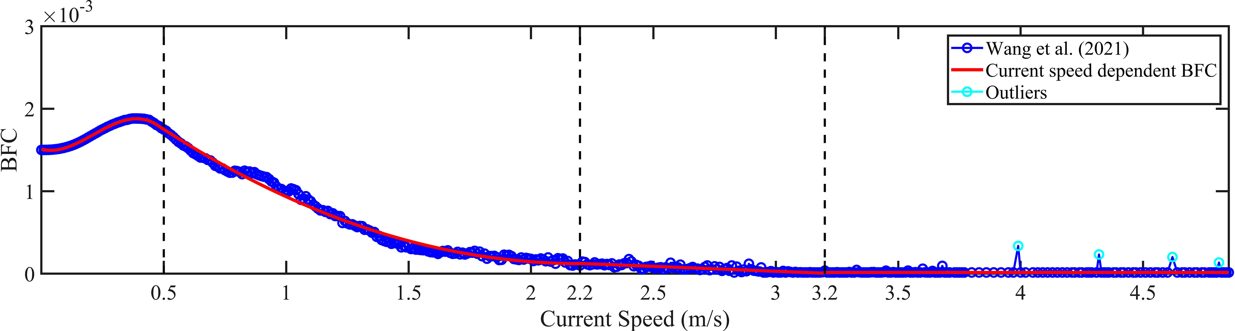
Figure 1 Relationship between BFC and current speed in Wang et al. (blue circle line) and the fitted empirical formula of BFC with a dependence on the current speed (red line). The light blue circles indicate the outliers and the black dashed lines indicate the breakpoints.

Based on the relationship between current speed and BFC obtained by Wang et al. (2021), we explored various approaches, including power, logarithmic, polynomial functions, and spatial fitting. Ultimately, we selected the polynomial fitting algorithm to propose a function describing the association of both variables in this study due to its superior fitting effect. Before fitting the data, outliers were removed, and the fitting interval was determined based on the trend of the curve. For the current speed range of 0-0.5 m/s, we opted for a cubic polynomial, as it demonstrated better fitting performance compared to a quadratic polynomial. In the range of 0.5-2.2 m/s, which exhibited a parabolic shape, a quadratic polynomial was employed for fitting, resulting in an R² value exceeding 0.9. Furthermore, for the range of 2.2-3.2 m/s, linear fitting outperformed other methods with an R² value above 0.7. Notably, when the current speed exceeded 3.2 m/s, one or several values significantly deviated from the rest, which were identified as outliers. In this case, the BFC was considered a constant of 0.000015. The resulting empirical formula of BFC with a dependence on the current speed was termed the “current speed-dependent BFC” and is presented below:

$\begin{array}{ll}k=\{\begin{array}{cc}(15.1-176.6s^3+113.1s^2-7.77983s)\times {10}^{-4},& s<0.5\\ (28.5+5.6376s^2-24.8s)\times {10}^{-4},& 0.5\le s<2.2\\ (3.86559-1.18963s)\times {10}^{-4},& 2.2\le s<3.2\\ 0.000015,& s\ge 3.2\end{array}& (1)\end{array}$

where s is the current speed (unit: m/s) and k is the BFC. As the current speed is spatially and temporally varying, the current speed-dependent BFC is also spatially and temporally variable.

3 Models

3.1 Two-dimensional multi-constituent tidal model

The governing equation of the two-dimensional (2D) depth-averaged multi-constituent tidal model is as follows (Wang et al., 2021):

$\begin{array}{ll}\frac{\partial \zeta }{\partial t}+\frac{1}{a}\frac{\partial [(h+\zeta )u]}{\partial \lambda }+\frac{1}{a}\frac{\partial [(h+\zeta )v\cos \varphi ]}{\partial \varphi }=0& (2)\end{array}$

$\begin{array}{ll}\frac{\partial u}{\partial t}+\frac{u}{a}\frac{\partial u}{\partial \lambda }+\frac{v}{R}\frac{\partial u}{\partial \varphi }-\frac{uv\tan \varphi }{R}-fv+\frac{ku\sqrt{u^2+v^2}}{h+\zeta }-A\Delta u+\frac{g}{a}\frac{\partial (\zeta -\overline{\zeta })}{\partial \lambda }=0& (3)\end{array}$

$\begin{array}{ll}\frac{\partial v}{\partial t}+\frac{u}{a}\frac{\partial v}{\partial \lambda }+\frac{v}{R}\frac{\partial v}{\partial \varphi }+\frac{u^2\tan \varphi }{R}+fu+\frac{kv\sqrt{u^2+v^2}}{h+\zeta }-A\Delta v+\frac{g}{R}\frac{\partial (\zeta -\overline{\zeta })}{\partial \varphi }=0& (4)\end{array}$

Where $\text{ζ }$ is the sea surface elevation above the undisturbed sea level; t is time; ϕ and λ are north latitude and east longitude, respectively; R is the radius of the Earth; a = Rcosϕ; h is the depth of water; u and v are the east-west and north-south velocity components, respectively; g is the gravitational acceleration; f is the parameter of Coriolis; k represents the BFC, which describes the bottom friction; A is the eddy viscosity coefficient in the horizontal direction, $\overline{\zeta }$ is the adjusted height of the equilibrium tide, which was calculated according to Fang et al. (1999) and Gao et al. (2015); and Δ is the Laplace operator, which is expressed as:

$\begin{array}{ll}\Delta (u,v)=a^{-1}\left[a^{-1}{\partial }_{\lambda }\left({\partial }_{\lambda }(u,v)\right)+R^{-1}{\partial }_{\varphi }\left(\cos \varphi {\partial }_{\varphi }(u,v)\right)\right]& (5)\end{array}$

At the solid boundary, the velocity components at normal direction are 0. At the open boundary, the variation of water elevation resulting from the tide is calculated as follows:

$\begin{array}{ll}\zeta (t)={\displaystyle \sum _{m=1}^M{F}_m{A}_m\cos \left({\omega }_{m}t+V_m+U_m-G_m\right)}& (6)\end{array}$

which involves various tidal parameters, including the amplitude (A), the phase lag (G) in UTC, the nodal factor (F), the initial phase angle (V) of the equilibrium tide, the nodal angle (U), the angular speed (ω) of the tidal constituent, the mth tidal constituent (m), and the number of tidal constituents (M). In addition, the discretization and scheme of the model are consistent with those shown in Lu and Zhang (2006).

3.2 Model settings

The study area was set to the BYECS with a horizon resolution of 1/6° × 1/6° (Figure 2). A time-step of 80s was chosen for the simulation. According to Fang (2004), the simulation included four fundamental constituents M₂, S₂, K₁, and O₁. And the open boundaries were selected along the Korean Strait, Tsushima Strait, Osumi Strait, Ryukyu Islands, Okinawa Trough, and Taiwan Strait (Figure 2). The tidal inversion software developed by Oregon State University was used to obtain the time series of tidal levels at the open boundary (Egbert and Erofeeva, 2002). The simulation was carried out for a period of 30 days, commencing from the static water state (ζ, u, v = 0) on 1 January 2010. The simulation in the first 15 days was sufficient to allow the simulated four tidal constituents to be stable (Cao et al., 2015). Consequently, the simulated results from the latter half of the simulation period (the last 15 days) were utilized for analysis, focusing on obtaining the simulated harmonic constants.

FIGURE 2

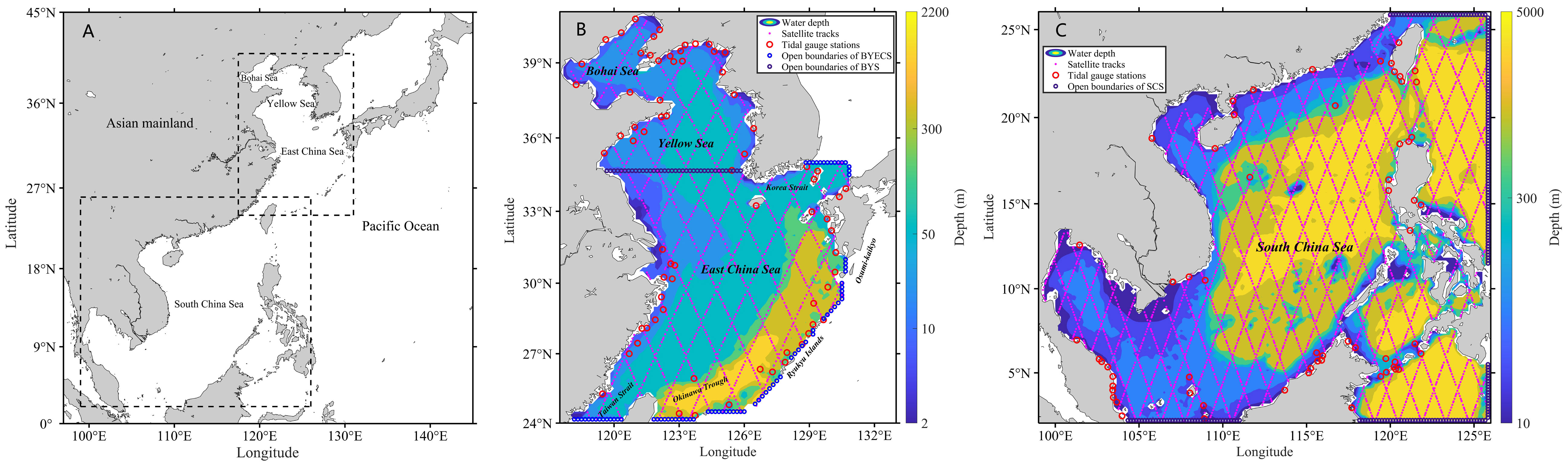
Figure 2 (A) Location of the BYECS and SCS (rectangle with dashed lines); (B) Water depths and positions of tidal gauge stations (red circles), T/P satellite tracks (pink dots), open boundaries of the BYECS (blue circles) and BYS (purple circles). (C) Same as (B) but for the SCS.

In this work, the accuracy of the numerical tidal simulation was evaluated using T/P satellite altimetry and tidal gauge data. T/P satellite altimetry data included tidal harmonic constant data (amplitude and phase lag) of the four fundamental tidal constituents (M₂, S₂, K₁, and O₁) from CTOH/LEGOS, France (http://ctoh.legos.obs-mip.fr), and the spatial distribution is shown in Figure 2. For coastal regions, tidal gauge stations, a traditional tool for obtaining tidal observations, provided accurate tidal information. The harmonic constants of four fundamental tidal constituents (M2, S2, K1, and O1) at coastal tidal gauge stations were obtained from Lu and Zhang (2006), and the distribution is shown in Figure 2. For coastal regions, tidal gauge stations, a traditional tool for obtaining tidal observations, provided accurate tidal information. The distribution of coastal tidal gauge stations is also shown in Figure 2. The accuracy of the numerical tidal simulation was analyzed by two metrics: the mean absolute error (MAE) and the vector error (VE) between the simulated harmonic constants and the observed results from T/P satellite altimeters and tide gauge stations. And the VE is calculated as follows (Fang, 2004):

$\begin{array}{ll}VE=\frac{1}{M}{\displaystyle \sum _{m=1}^M\sqrt{{\left({\overline{A}}_m\cos {\overline{G}}_m-A_m\cos G_m\right)}^2+{\left({\overline{A}}_m\sin {\overline{G}}_m-A_m\sin G_m\right)}^2}}& (7)\end{array}$

where VE is the vector error for one tidal constituent; $\overline{A}$ (A) and $\overline{G}$ (G) are the observed (simulated) amplitude and phase lag of this tidal constituent; and M is the number of observations.

4 Benchmark experiments

4.1 Experimental design

In order to evaluate the newly proposed empirical formula of BFC, the group of numerical experiment E1 was designed to compare it with the other widely used parameterization schemes of BFC in the BYECS. In numerical experiment E1-1, BFC was set as a constant value of 0.0015 in the BYECS (Lee and Jung, 1999), which was referred to as “constant BFC”. In numerical experiment E1-2, BFC was set with a form related to water depth, as used in Kang et al. (1998). In detail, BFC was defined as k=g/C²=gn²/h^1/3, where g is the acceleration due to gravity, as above; C is the Chezy coefficient, and n is Manning’s n coefficient and set as 0.023 (Herrling and Winter, 2015; Mardani et al., 2020), its unit is s/m^1/3. This empirical formula of BFC has been widely applied in ocean models, such as FVCOM, and was referred to as “Chezy-Manning BFC”. In numerical experiment E1-3, BFC was related to water depth according to the relationship between the estimated BFC and water depth in the BYECS obtained from Wang et al. (2021), as shown in Figure 3. The fitted relationship between BFC and water depth is shown in Equation (8) and Figure 3, with R² of 0.89 for the 110 m-600 m segment and R² above 0.9 for the other segments. The empirical formula of BFC used in E1-3 was called “depth-dependent BFC”. In numerical experiment E1-4, the new empirical formula of BFC named “current speed-dependent BFC” was used. In all the above numerical experiments numbered with the prefix of “E1”, four basic tidal constituents M₂, S₂, K₁, and O₁ were simulated in the BYECS. The specific model setup configurations for those experiments are provided in Table 1.

FIGURE 3

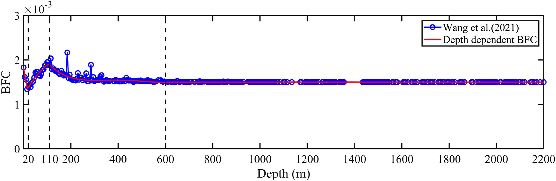
Figure 3 Relationship between BFC and water depth in Wang et al. (blue circle line) and the fitted curve (red line). The black dashed lines indicate the interval end points.

TABLE 1

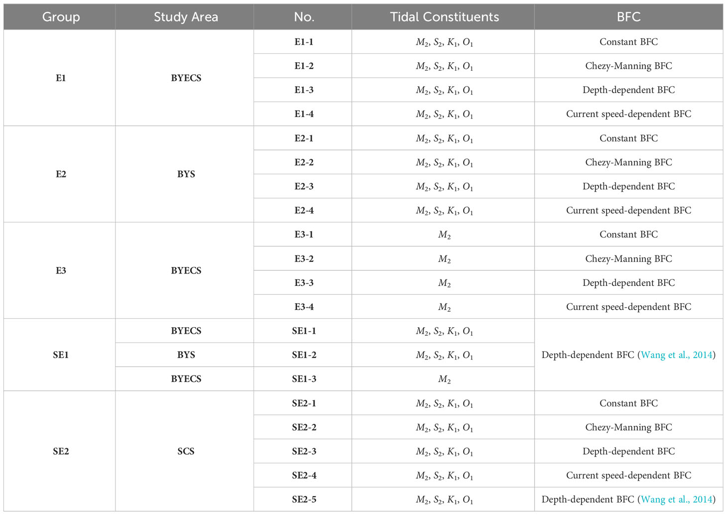
Table 1 Design of numerical experiments.

$\begin{array}{ll}k=\{\begin{array}{cc}(182-3.06225h)\times {10}^{-5},& h<20\\ (120+0.956677h-0.00272459h^2)\times {10}^{-5},& 20\le h<110\\ 0.00293+(0.0530021h^4-89.7801h^3+54894.9h^2-14447500h)\times {10}^{-12},& 110\le h<600\\ 0.0015,& h>600\end{array}& (8)\end{array}$

where h is the depth of water and k is the parameter BFC.

4.2 Experimental results

The simulated results in the experiment group E1 were compared with the satellite altimetry and tidal gauge data, and the results are presented in Table 2. As shown in Table 2, most results of numerical experiment E1-2 have the largest deviation from the satellite altimetry data. The VEs for the M₂, S₂, K₁, and O₁ tides are 21.54 cm, 8.21 cm, 3.81 cm, and 4.78 cm, which are larger than the other three experiments except for O1 in E1-3. The mean of VEs (MVE) of the simulated tidal constituents in E1-2 is 9.59 cm, which is the largest among all experiments, indicating that the simulated results obtained using Chezy-Manning BFC have the largest error. The VEs of the four tidal constituents in E1-4 are 19.83 cm, 7.52 cm, 3.41cm, and 4.47 cm, respectively. The MVE in E1-4 is 8.81 cm, which is decreased by 3.6%, 8.1%, and 1.0% compared to E1-1, E1-2, and E1-3, respectively. The above results show that the current speed-dependent BFC will improve the simulation accuracy of tides in the BYECS. As listed in Table 2, when compared to the tidal gauge data, the VEs for M₂, S₂, K₁, and O₁ in E1-2 are 28.18 cm, 11.16 cm, 5.53 cm, and 7.07 cm, respectively, which are much larger than those in other experiments. The VEs for M₂, S₂, K₁, and O₁ in E1-4 are 22.55 cm, 9.03 cm, 4.81 cm, and 6.10 cm, respectively, and all of them are less than those in other experiments. The MVE in E1-4 is 10.62 cm, which is less than 12.21 cm in E1-1, 12.98 cm in E1-2, and 12.09 cm in E1-3, showing again that the current speed-dependent BFC will improve the simulation accuracy of tides in the BYECS. Although the MVE is decreased by only 1 cm compared with the tidal gauge data, the simulation accuracy in E1-4 is improved by 18.2% compared to that in E1-2. The aforementioned results indicate that the current speed-dependent BFC proposed in this study is much more reasonable than the other schemes of BFC in the BYECS. The MVE for tidal gauge data after data assimilation in Wang et al. (2021) is just 6.90 cm and much less than 10.62 cm in E1-4, as the current speed-dependent BFC in E1-4 is in fact the smoothing and simplified result of the freely estimated BFC in Wang et al. (2021). As the estimated spatially and temporally varying BFC in Wang et al. (2021) cannot be used for other tidal models and other areas, the current speed-dependent BFC in E1-4 has the advantage to be widely used and decrease the simulation errors for other models and other areas.

TABLE 2

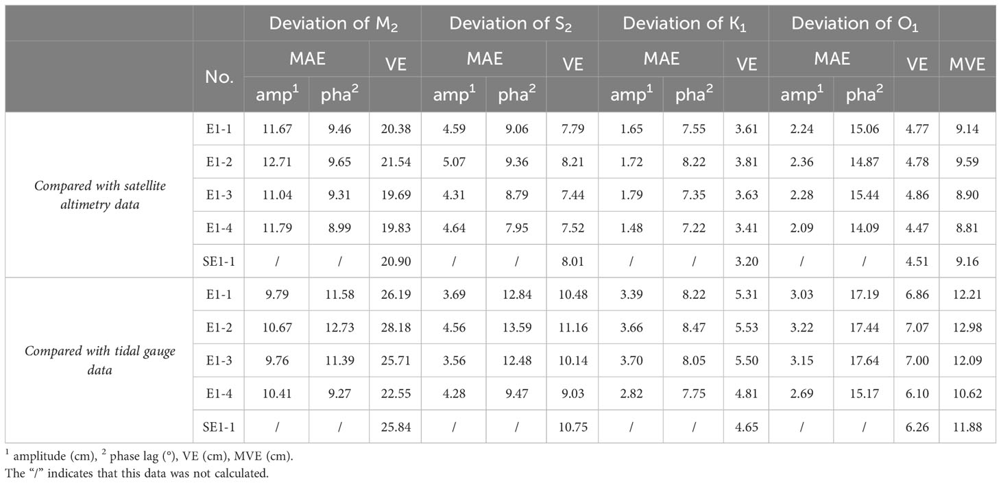
Table 2 Deviation of simulation results for M₂, S₂, K₁, and O_1..

Figure 4 shows the MVE between the simulated results in four experiments in E1 and tidal gauge data. The proportion of MVE ≤ 10cm in E1-4 is about 31%, which is significantly larger than those in E1-1, E1-2, and E1-3. The cumulative percentage of MVE ≤ 30cm and MVE ≤ 40cm in E1-4 are 70% and 87%, respectively, which are also significantly larger than those in the other three experiments. The above results show that the current speed-dependent BFC can increase the quantity of small MVEs while decreasing the number of large MVEs to improve the overall simulation accuracy. Figure 5 shows the MVE between the simulated results of the four experiments of Group E1 and the observation at each tidal gauge station in the BYECS. At most of the tidal gauge stations, the MVEs in E1-4 are not larger than those in E1-1, E1-2, and E1-3. In particular, at the tidal gauge stations numbered 4, 12, 18, 20, 21, 24, 25, 30-33, 36-38, and 41-45, the MVEs in E1-4 are significantly less than those in the other three experiments. The stations of the tide gauge where the simulation results obtained using the current speed-dependent BFC outperform the other three schemes are referred to as the improved stations. As shown in Figure 6, the improved stations in the Group E1 experiments are primarily located in the eastern part of the Bohai Sea, the Yellow Sea, off Hangzhou Bay, and near the Korean Strait.

FIGURE 4

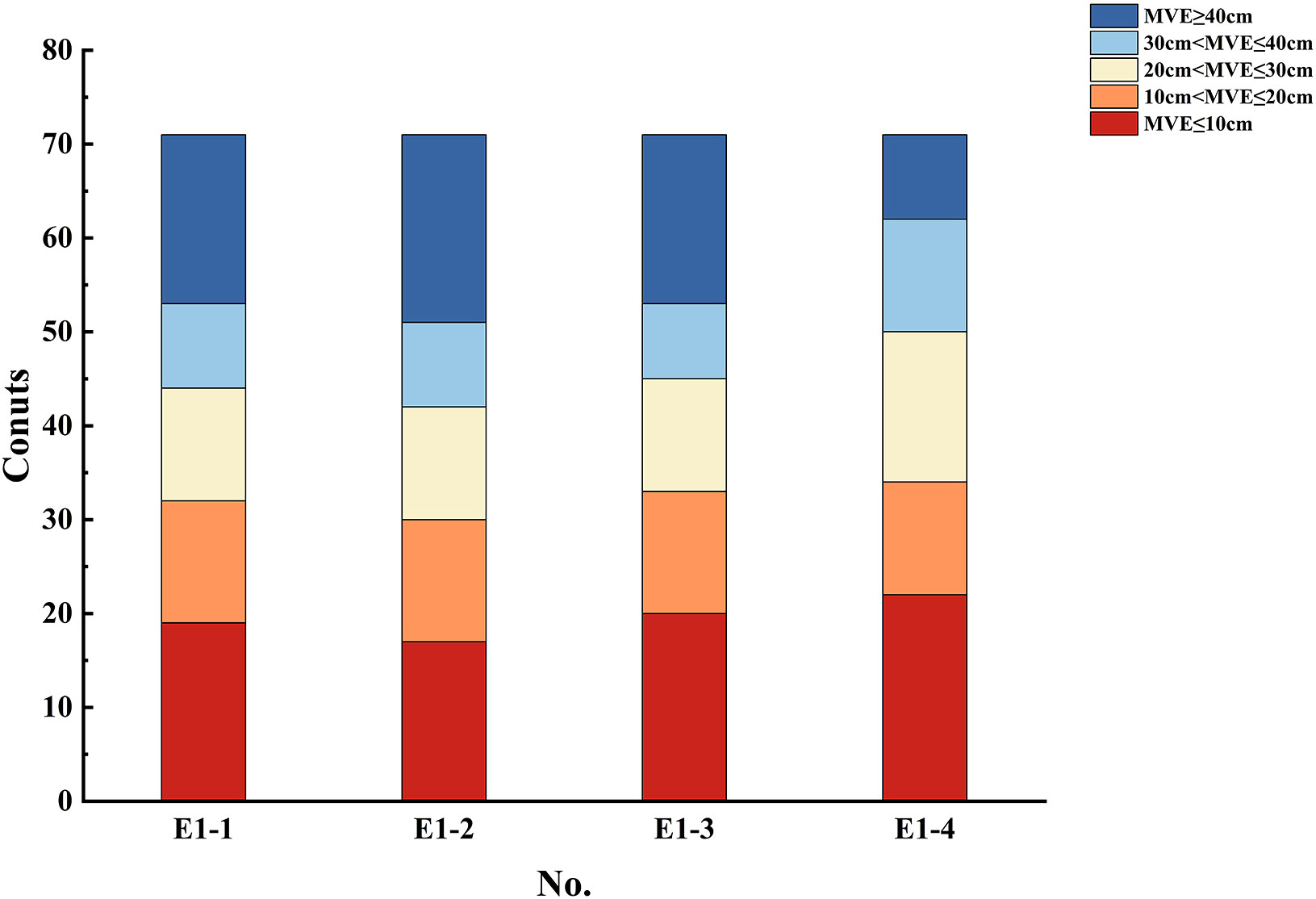
Figure 4 Distribution of the MVE between the simulated results and tidal gauge data in E1-1, E1-2, E1-3, and E1-4.

FIGURE 5

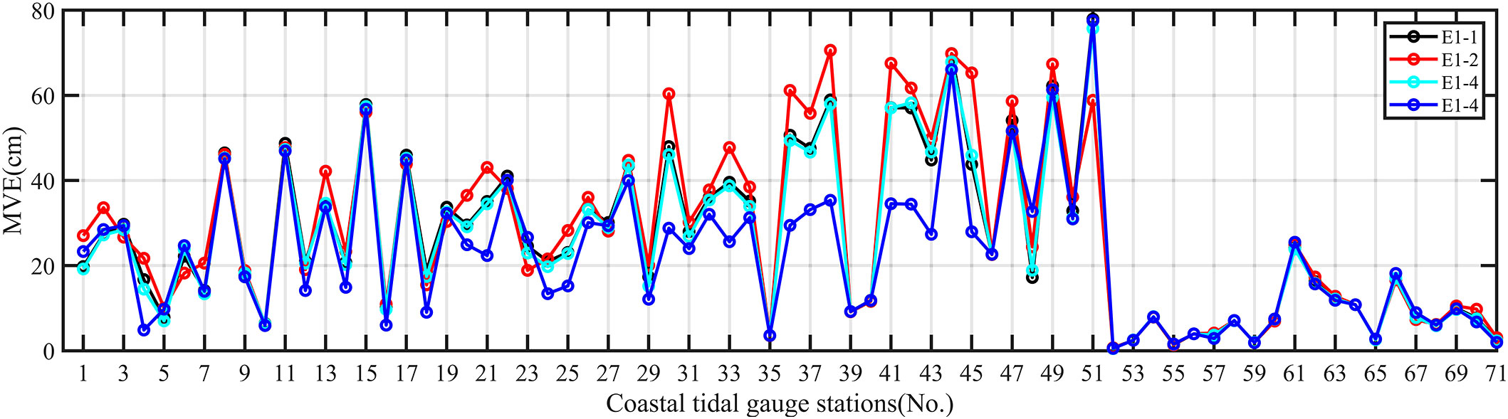
Figure 5 MVE between the simulated results and each tidal gauge station data in E1-1, E1-2, E1-3, and E1-4.

FIGURE 6

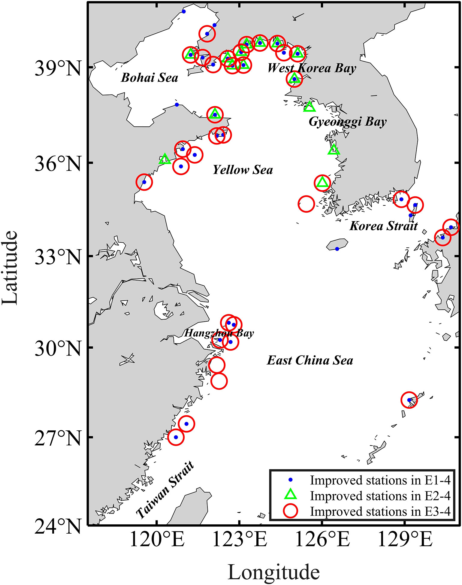
Figure 6 Distribution of the improved stations in E1-4, E2-4, and E3-4.

In summary, the simulation results for the four basic tidal constituents in E1-4 come closest to the satellite altimetry and tidal gauge data, indicating that the current speed-dependent BFC is more reasonable than the constant BFC, Chezy-Manning BFC, and depth-dependent BFC. Specifically, the scatterplot in Figure 7 illustrates that over 95% of the amplitude and phase lag calculated from the E1-4 simulation results fall within the range of 0.5 to 2 times those obtained from the tidal gauge observations. The correlation coefficients between the observed harmonic constants and the corresponding simulations for the four tidal constituents are at least 0.90. Similarly, the comparison between the E1-4 simulation and the satellite altimetry data (Figure 7) leads to a similar conclusion and the correlation coefficients between them are not less than 0.88. The cotidal charts of the four tidal constituents in E1-4 (Figure 8) show the same pattern as those in Fang (2004) and Wang et al. (2021) in terms of the distribution of amphidromous points, amplitudes, and co-phase lines. Furthermore, the tidal ellipses of the four tidal constituents obtained in E1-4 (Figure 9) are generally in agreement with the results in Fang (1994); Guo and Yanagi (1998), and Wang et al. (2021). These findings further demonstrate that the current speed-dependent BFC leads to improved simulation results for the four tidal constituents in the BYECS. Collectively, the aforementioned results provide strong evidence that the current speed-dependent BFC proposed in this study is considerably more reasonable compared to the other three empirical formulas of BFC, resulting in significantly improved simulated results for multi-constituent tides in the BYECS.

FIGURE 7

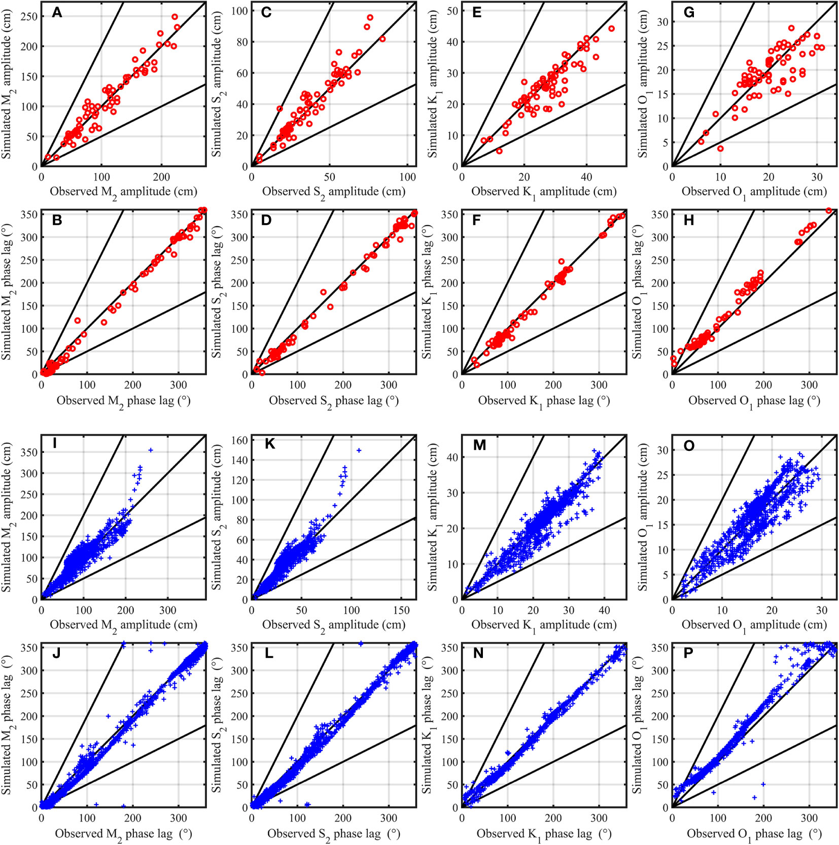
Figure 7 Comparison of simulated results and tidal gauge data in E1-4 (red circle): (A) M₂ amplitude, (B) M₂ phase lag, (C) S₂ amplitude, (D) S₂ phase lag, (E) K₁ amplitude, (F) K₁ phase lag, (G) O₁ amplitude, and (H) O₁ phase lag. And comparison of simulated results and satellite altimetry data in E1-4 (blue plus): (I) M₂ amplitude, (J) M₂ phase lag, (K) S₂ amplitude, (L) S₂ phase lag, (M) K₁ amplitude, (N) K₁ phase lag, (O) O₁ amplitude, and (P) O₁ phase lag. For reference, the 1:1, 1:2, and 2:1 lines are shown in all figures (solid black line).

FIGURE 8

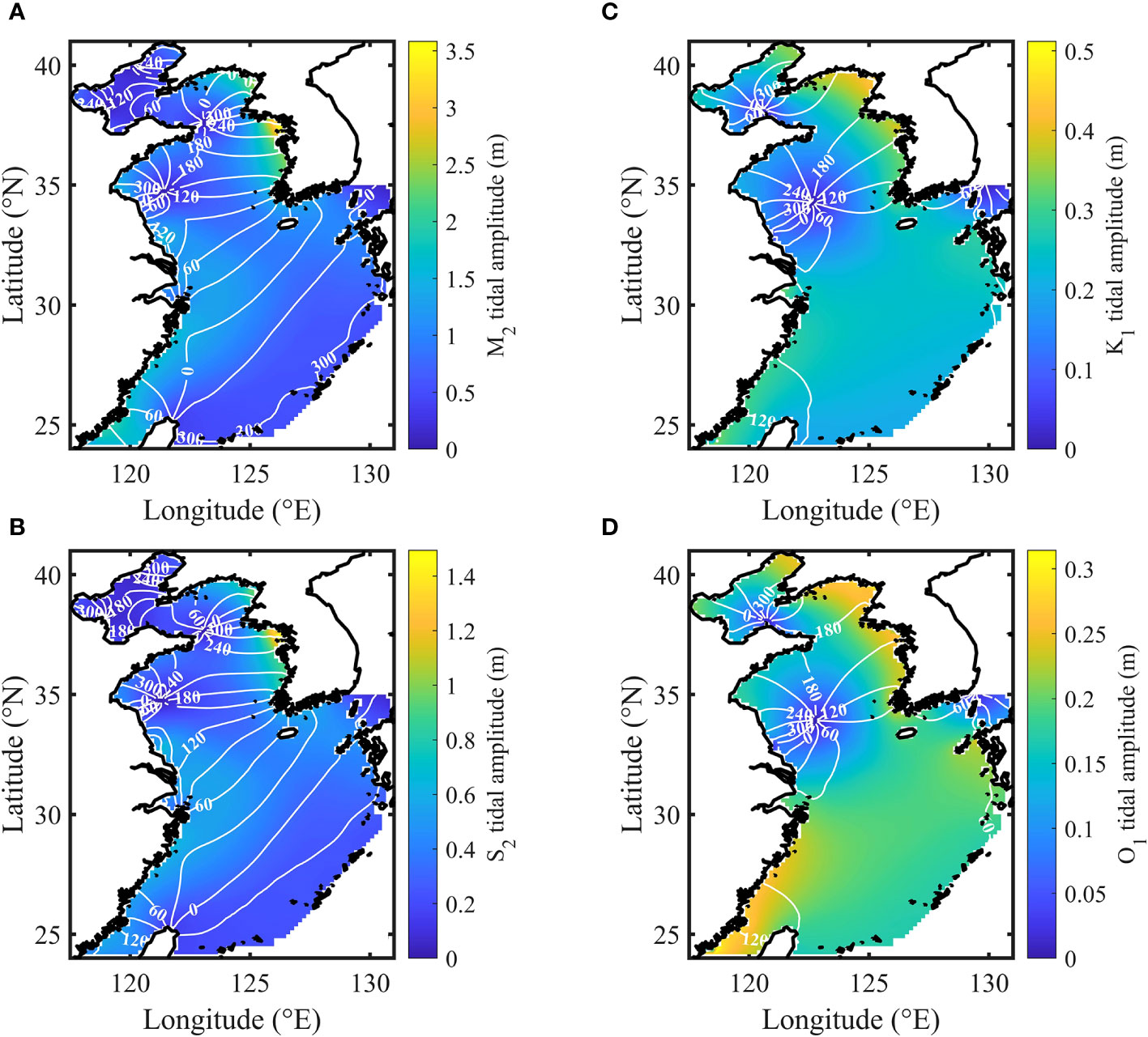
Figure 8 Cotidal charts for (A) M₂, (B) S₂, (C) K₁ and (D) O₁ in the BYECS obtained in E1-4, where the colored shading and white lines indicate amplitude and phase lag, respectively.

FIGURE 9

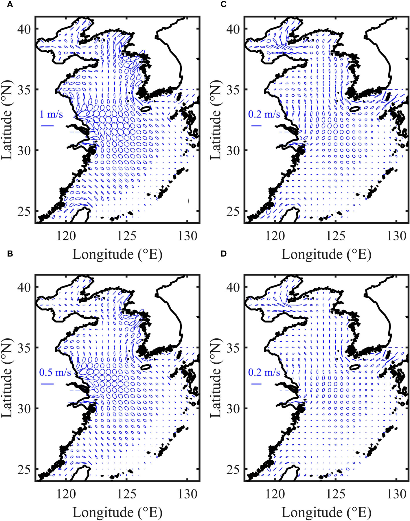
Figure 9 Tidal current ellipses for (A) M₂, (B) S₂, (C) K₁ and (D) O₁ in the BYECS obtained in E1-4.

5 Discussions

It is necessary to be noted that the newly proposed empirical formula of current speed-dependent BFC is based on the fitted results of the spatially-temporally varying BFC versus the current speed obtained by Wang et al. (2021) in the BYECS. Thus, it is unsurprising that the current speed-dependent BFC performs well in simulations of M₂, S₂, K₁, and O₁ in the same region. In the discussions, the current speed-dependent BFC was applied to simulate four tidal constituents in the BYS, only M₂ in the BYECS, and four tidal constituents in the South China Sea (SCS) to further investigate the applicability and advantages of this new empirical formula. Furthermore, the spatial and temporal distribution of BFC obtained using this new empirical formula were also discussed.

5.1 Application in the simulation of four tidal constituents in the BYS

In the group of sensitivity experiment E2, simulations of the four main tidal constituents were carried out in the BYS to evaluate the applicability of different BFC schemes. The constant BFC, Chezy-Manning BFC, depth-dependent BFC, and current speed-dependent BFC were used in experiments E2-1 to E2-4, respectively. Some specific model settings for those experiments are shown in Table 1, and the rest of the settings were consistent with those of experiment E1.

The simulated results of sensitivity experiment E2 were compared with the satellite altimetry and tidal gauge data, as shown in Table 3. The MVE between simulation results and tidal gauge data in E2-4 is 10.61cm, which is less than 11.13 cm in E2-1, 11.87 cm in E2-2, and 11.17 cm in E2-3, amounting to an improvement of at least 4.7%. Specifically, VEs for all the four tidal constituents in E2-4 are less than those in E2-1, E2-2, and E2-3, of which the E2-2 results obtained with Chezy-Manning BFC show the largest error. As shown in Figure 6, improved stations in E2-4 account for about half of all gauge stations used for verification in the BYS, mostly located in coastal areas such as the Gulf of Korea and Gyeonggi Bay.

TABLE 3

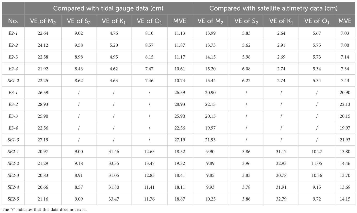
Table 3 Comparison of the simulated and observed results of the four principal tidal constituents.

In addition, the MVE between the simulation results and the T/P satellite altimetry data in E2-4 is larger than those in E2-1, E2-2, and E2-3 by 4.4%, 4.9%, and 2.8% (Table 3), respectively. It should be pointed out that the BYS is shallow waters with a maximum depth of about 100 m. Shum et al. (1997) indicated that tidal root mean square accuracies derived from satellite altimetry data were within 2-3 cm in deeper waters, but their uncertainty increased significantly in coastal areas or near shallow seas. The reason is that satellite altimeter data exhibits geographical variability in shallow water compared to open oceans (Fok et al., 2010), and they may also be affected by factors such as coastline and topography (Cherniawsky et al., 2001) as well as tropospheric and ionospheric correction models (Lyard et al., 2006; Desportes et al., 2007). Xu and Chen (2021) characterized the global ocean tides using altimeter data and found that the amplitude deviation of the M₂ tide could reach 7.49 cm where water depths were less than 200 m, but the deviation was only 2.15 cm in deeper waters. Taking into consideration the uncertainty of satellite altimetry data in shallow water, the negligible difference in the MVEs between the simulation results and the satellite altimetry data in these experiments could be ignored.

Overall, when simulating the four principal tidal constituents in the BYS, the current speed-dependent BFC proposed in this paper leads to smaller simulation errors than the constant BFC, Chezy-Manning BFC, and depth-dependent BFC in the MVEs between the simulated results and tidal gauge data, indicating that this new empirical formula of BFC is applicable in other sea areas.

5.2 Application in the simulation of only M₂ tide in the BYECS

In the group of sensitivity experiment E3, only the tidal constituent M₂ was simulated in the BYECS to compare the applicability of different schemes of BFC for simulating different tidal constituents. In sensitivity experiments E3-1 to E3-4, the constant BFC, the Chezy-Manning BFC, the depth-dependent BFC, and the current speed-dependent BFC were used, respectively. Some model preferences of those experiments are presented in Table 1. The remaining model setups were consistent with those in experiment E1.

As listed in Table 3, the simulated results were compared with the T/P satellite altimetry and tidal gauge data. The MVE between simulated results and tidal gauge data in E3-4 is 22.56 cm, which is significantly less than those of 26.59 cm in E3-1, 28.93 cm in E3-2, and 25.90 cm in E3-3, amounting to an improvement of at least 12.90%. Comparison between simulation and T/P satellite altimetry data shows similar results: the MVE in E3-4 is 19.97cm, which is less than 20.90 cm, 22.13 cm, and 20.15 cm for other three schemes. The above results indicate that, on the whole, the simulated results of M₂ tide in the BYECS using the current speed-dependent BFC are much closer to both the tidal gauge data and the satellite altimetry data than others. The details of MVE for each experiment in E3 is shown in Figure 10. The tidal gauge stations with MVE less than or equal to 40 cm account for 87.3% of the total number of tidal gauge stations in E3-4, while those are 76.1% in E3-1, 69.0% in E3-2, and 76.1% in E3-3, indicating that the number of tidal gauge stations with large MVE significantly decreases. Meanwhile, the cumulative proportions of MVE less than or equal to 10 cm, less than or equal to 20 cm and less than or equal to 30 cm at the tide gauge stations in E3-4 are larger than the other three experiments. As shown in Figure 6, at most of the tide gauge stations, the simulation of the M₂ tide using the current speed-dependent BFC in the BYECS in E3-4 are improved compared with the other schemes of BFC, especially in the Yellow Sea and the south of Hangzhou Bay. Moreover, the locations of improved stations in E3-4 are similar to those in the BYECS in E1-4 and in the BYS in E2-4, showing that the improvement of the newly proposed empirical formula of BFC is not limited to certain simulated areas or tidal constituent. The newly proposed empirical formula of BFC is also applicable to simulation of only M₂ tide in the BYECS.

FIGURE 10

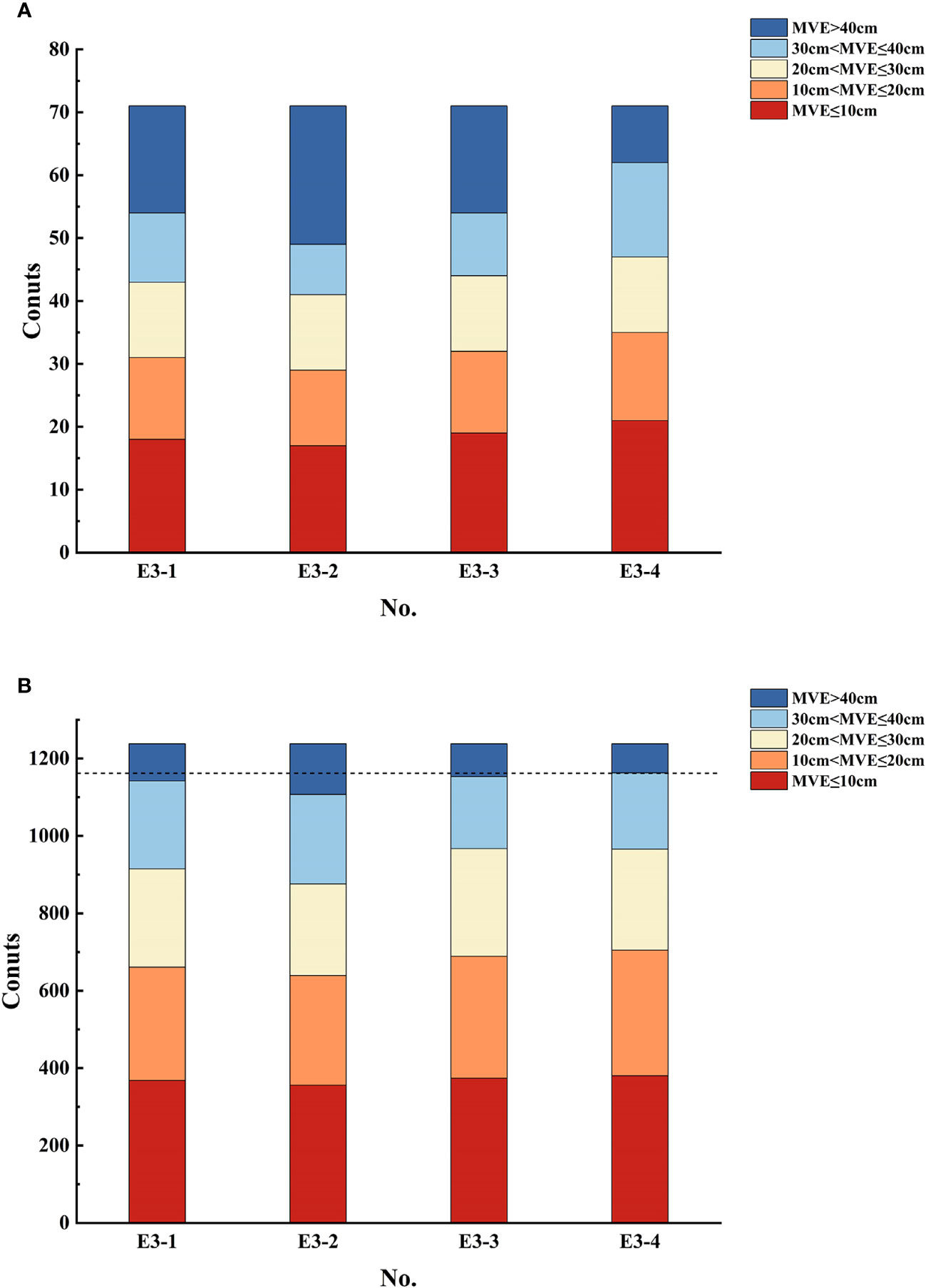
Figure 10 Distribution of MVE between (A) the simulated results and tidal gauge data, (B) the simulated results and satellite altimetry data in sensitivity experiments E3-1 to E3-4.

5.3 Comparison with the spatial variation of BFC explained by water depth

The study of spatially varying BFC obtained through data assimilation was previously conducted by Wang et al. (2014), and an empirical formula derived from optimal fitting was found to yield superior results for M₂ tidal simulation. Therefore, we included this scheme for analysis and comparison, as shown in Table 1. Wang et al. (2014) focused on the quantitative relationship between BFC and water depth when the water depth is below 100 m. The fitting function in Wang et al. (2014) is as follows:

$\begin{array}{ll}k=\{\begin{array}{ll}1.5363\times {10}^{-3},\hfill & h\ge 100\hfill \\ (56.8850+0.9674h)\times {10}^{-5},\hfill & 30\le h<100\hfill \\ (100.0-0.5413h)\times {10}^{-5},\hfill & h<30.\hfill \end{array}& (9)\end{array}$

Where k is the BFC and h is the water depth. In a similar manner, we incorporated this scheme as the fifth BFC scheme and conducted simulations in the base experiment (SE1-1) as well as two sets of sensitivity experiments (SE1-2 and SE1-3), while maintaining the remaining model conditions unchanged. The simulation results are presented in Tables 2, 3.

As shown in Table 1, the MVE between the simulated results and the tidal gauge (satellite altimetry data) is 11.88 cm (9.16 cm) in SE1-1 using the depth-dependent BFC in Wang et al. (2014), which is much larger than those in E1-4 using the proposed current speed-dependent BFC. When four tidal constituents were simulated in the BYS, the simulated results in SE1-2 using the depth-dependent BFC in Wang et al. (2014) are much far from both the tidal gauge data and satellite altimetry data than the simulated results using the current speed-dependent BFC in E2-4, as listed in Tables 2, 3. The similar result is also obtained when only M₂ tide was simulated in the BYECS. From the experimental results, the depth-dependent BFC in Wang et al. (2014) has an advantage over the Chezy-Manning scheme in terms of its ability to simulate the M₂, but its simulation error is still higher than that of the newly proposed current speed-dependent BFC scheme.

5.4 Application in the simulation of four tidal constituents in the SCS

The above experiments were implemented only in the BYECS, so the SCS was selected as a separate study area to verify the different schemes of BFC. Another group of sensitivity experiments (SE2) was set up in the SCS. The model boundaries and distribution of validation data are shown in Figure 2C, and the model setup remained unchanged except for the experimental region. The four principal tidal constituents (M₂, S₂, K₁, and O₁) were simulated in the SCS with five different schemes of BFC, as listed in Table 1.

From Table 3, the MVE between the tidal gauge data and the simulated results in SE2-1, SE2-2, SE2-3, SE2-4, and SE2-5 are 18.52 cm, 19.32 cm, 18.41 cm, 18.11 cm, and 18.87 cm, respectively, indicating that the smallest simulated error was achieved when the current speed-dependent BFC was used in SE2-4. Similarly, the MVE between the satellite altimetry data and the simulated results in SE2-4 is less than those in other experiments. The aforementioned results show that the proposed current speed-dependent BFC is also preferable than the other schemes of BFC in the SCS, further demonstrating the superiority of the current speed-dependent BFC proposed in this study.

In terms of MVE performance, despite the new formula’s improvement capability within 1cm, it still provides an enhancement of about 10% in the tidal gauge data, both in BYECS and in the sensitive experiments of SCS. In addition, as can be seen from the histograms in Figures 4, 10, the discrepancy of the simulation results of the new formula can be effectively reduced.

In physical terms, the new formula produces result that closely align with the observed behavior of the BFC in relation to current speed (Cheng et al., 1999; Wang et al., 2004; Safak (2016); Fan et al., 2019). Furthermore, in practical scenarios where the current speed undergoes temporal variations, such as in pipes or oceans, the Reynolds number of the current changes, and consequently, the current regime may also change. It is reasonable to believe that this introduces a potential time variation in the friction factor.

5.5 Spatial and temporal distributions of the current speed-dependent BFC

The BFC is of great importance for numerical simulations in shallow waters and must be accurately set. The new empirical formula of BFC with a dependence on the current speed in this paper yields better results than the constant BFC, the Chezy-Manning BFC, and the depth-dependent BFC in the simulation of four principal tidal constituents in both the BYECS and the BYS, and the single tidal constituent M₂ in the BYECS. Therefore, the spatial and temporal distributions of BFC in the BYECS obtained using the new empirical formula were analyzed.

The spatially and temporally varying BFC calculated using the empirical formula of BFC with a dependence on the current speed and the simulated sea surface elevation in E1-4 is spatially averaged in the BYECS to obtain the temporal distribution, which is displayed in Figure 11A. The period of temporal variation of spatially averaged sea surface elevation is roughly half-day, which is about twice as long as the BFC variation, consistent with the findings in Wang et al. (2021). Furthermore, it is worth noting that the spatial average of BFC exhibits considerable variability in response to tidal range. As can be seen in Figure 11B, the temporal variability of spatially averaged BFC in E1-4 is akin to that of spatially averaged current speed in terms of both frequency and trend, exhibiting a correlation coefficient of 0.46. The positive correlation is mainly attributed to the fact that the current speed ranges from 0 to 0.2 m/s where BFC increases with the increased current speed as shown in Equation (1) and Figure 1.

FIGURE 11

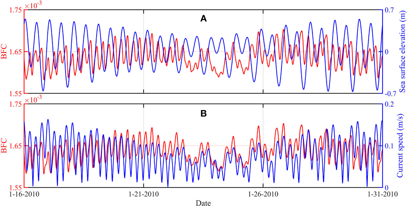
Figure 11 (A) Time series of spatially averaged BFC (red line) and sea surface elevation (blue line), and (B) time series of spatially averaged BFC (red line) and current speed (blue line) in E1-4.

Figure 12 displays the spatial distribution of the BFC that has been averaged over time and the current speed in E1-4. The mean current speed is relatively larger along the coast of Hangzhou Bay, West Korea Bay, and Gyeonggi Bay, where the BFC is lower than 0.0016. The temporally averaged BFC is small in the coastal regions near Hangzhou Bay, the Yangtze Estuary, and Gyeonggi Bay, which agrees with the pattern shown in Wang et al. (2014) and Lu and Zhang (2006). Furthermore, the analysis reveals the presence of local minimums in BFC, approximately around 0.0015, near the amphidromous points in the Bohai Sea and Yellow Sea. And relatively small values of BFC are observed in West Korea Bay and Gyeonggi Bay. In contrast, BFC remains relatively constant in the Okinawa Trough and open waters, potentially attributed to the stability of current speeds on a temporal scale.

FIGURE 12

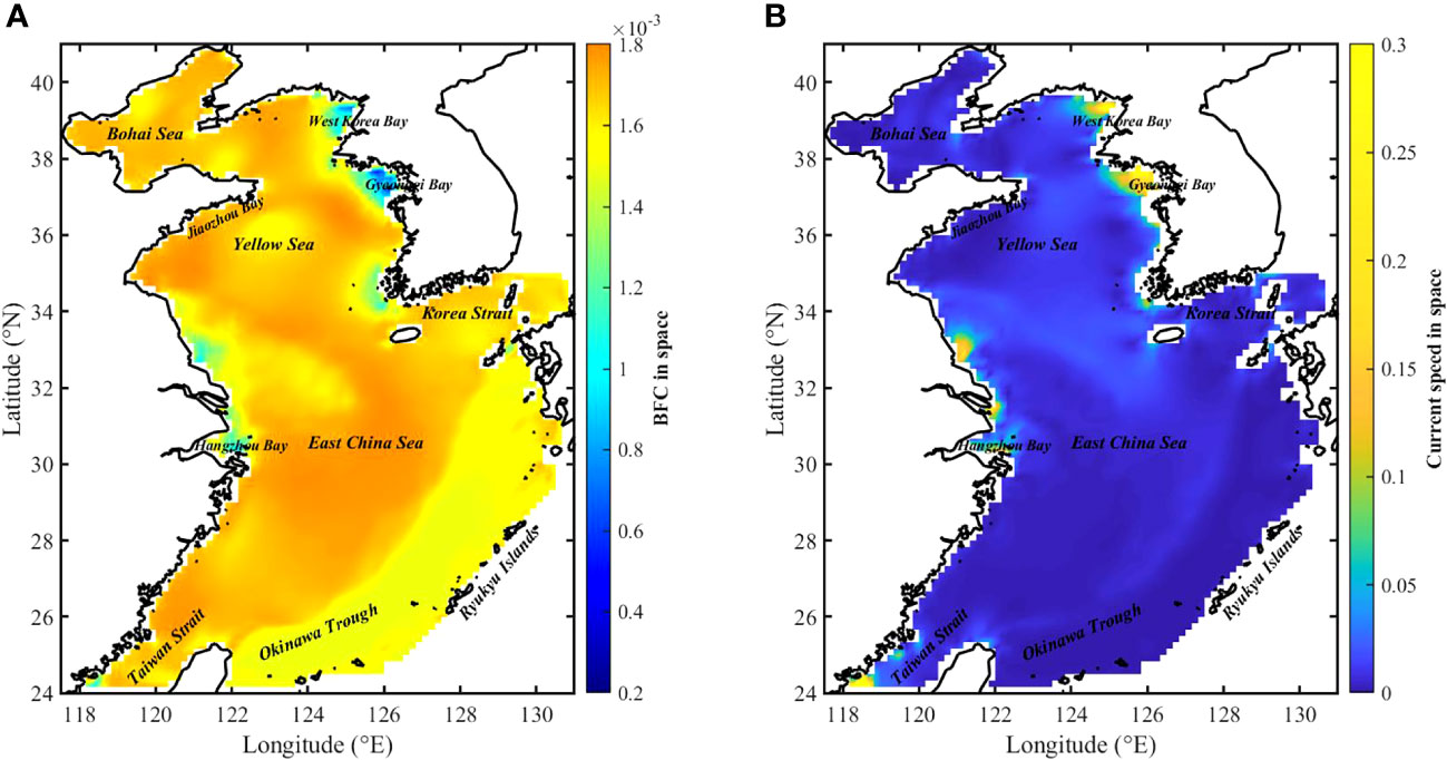
Figure 12 (A) Spatial distribution of temporally averaged BFC, and (B) spatial distribution of temporally averaged current speed in E1-4.

6 Conclusions

The accurate determination of BFC is essential for the simulation, forecasting, and analysis of tides and sediment transport. Extensive observational studies have consistently demonstrated that BFC exhibits spatial and temporal variability and is influenced by the current speed. However, incorporating the spatial and temporal variations of BFC into oceanographic models poses significant challenges. Based on the relationship between the spatially and temporally varying BFC and current speed obtained by Wang et al. (2021), a new empirical function of current speed-dependent BFC is proposed and compared with several traditional methods, including constant BFC, Chezy-Manning BFC and depth-dependent BFCs.

When simulating the four main tidal constituents in the BYECS, the MVE between the simulated results and the T/P satellite altimetry data in E1-4, in which the current speed-dependent BFC is used, is 8.81 cm and much less than those in other experiments. In addition, the number of the large MVE between the simulated results and the tidal gauge data in E1-4 is significantly decreased, resulting in the MVE in E1-4 being 10.62 cm and the model performance is improved by at least 10.6% compared to the other experiments. Furthermore, the simulated results in E1-4 captured the features of the tides and tidal currents in the BYECS. Similarly, whether simulating the four principal tidal constituents in the BYS, only the M₂ tide in the BYECS and four principal tidal constituents in the SCS, the simulated results obtained using the current speed-dependent BFC are much closer to the tidal gauge data than those using the other empirical formulas of BFC. The results of this paper indicate that the current speed-dependent BFC is much more applicable and reasonable than the constant BFC, the Chezy-Manning BFC, and depth-dependent BFCs.

The current speed-dependent BFC, which is newly proposed in this study, can reflect the influence of current speed on BFC and show the spatial and temporal characteristics of BFC. So, it has much more meaningful in physical terms than the traditional schemes and it is much easier access than the parameter estimation by using data assimilation. It is much superior to the traditional empirical formula of BFC and provides a new option for the setting of BFC in the tidal model. In the future, the effect of current speed-dependent BFC on the research of temporally varying mixing and energy will be further studied.

Data availability statement

Publicly available datasets were analyzed in this study. This data can be found here: http://ctoh.legos.obs-mip.fr.

Author contributions

JJ designed the original ideas. YD performed the numerical experiments and analyses. JJ, YD and DW contributed to the concept of the manuscript. YD wrote the original manuscript, JJ, XL, DW and JZ revised and improved the manuscript. All authors contributed to the article and approved the submitted version.

Funding

This research was funded by Open Funds for Key Laboratory of Marine Environmental Survey Technology and Application, Ministry of Natural Resources (grant number MESTA-2021-A004), Fund of Guangxi Key Laboratory of Beibu Gulf Marine Resources, Environment and Sustainable Development (grant number MRESD-2023-B02), Guangdong Basic and Applied Basic Research Foundation (grant number 2023A1515011262), National Natural Science Foundation of China (grant number 42106033, 42176172, 41876086), Hubei Provincial Natural Science Foundation of China (grant number 2023AFB002), Open Funds for Hubei Key Laboratory of Marine Geological Resources, China University of Geosciences (grant number MGR202102), and Open Funds for Teaching Laboratory, China University of Geosciences (grant number SKJ2022116).

Conflict of interest

The authors declare that the research was conducted in the absence of any commercial or financial relationships that could be construed as a potential conflict of interest.

Publisher’s note

All claims expressed in this article are solely those of the authors and do not necessarily represent those of their affiliated organizations, or those of the publisher, the editors and the reviewers. Any product that may be evaluated in this article, or claim that may be made by its manufacturer, is not guaranteed or endorsed by the publisher.

References

An H. S. (1977). A numerical experiment of the M2 tide in the Yellow sea. J. Oceanogr. Soc. Japan 33, 103–110. doi: 10.1007/BF02110016

CrossRef Full Text | Google Scholar

Blakely C. P., Ling G., Pringle W. J., Contreras M. T., Wirasaet D., Westerink J. J., et al. (2022). Dissipation and bathymetric sensitivities in an unstructured mesh global tidal model. J. Geophys. Res.: Oceans 127, e2021JC018178. doi: 10.1029/2021jc018178

CrossRef Full Text | Google Scholar

Cao A. Z., Wang D. S., Lv X. Q. (2015). Harmonic analysis in the simulation of multiple constituents: determination of the optimum length of time series. J. OF ATMOSP. AND OCEAN. Technol. 32, 1112–1118. doi: 10.1175/JTECH-D-14-00148.1

CrossRef Full Text | Google Scholar

Cheng R. T., Ling C. H., Gartner J. W., Wang P. F. (1999). Estimates of bottom roughness length and bottom shear stress in South San Francisco Bay, California. J. OF GEOPHYS. RESEARCH-OCEANS 104, 7715–7728. doi: 10.1029/1998JC900126

CrossRef Full Text | Google Scholar

Cherniawsky J. Y., Foreman M. G. G., Crawford W. R., Henry R. F. (2001). Ocean tides from TOPEX/poseidon sea level data. J. Atmosp. Ocean. Technol. 18, 649–664. doi: 10.1175/1520-0426(2001)018<0649:OTFTPS>2.0.CO;2

CrossRef Full Text | Google Scholar

Demissie H. K., Bacopoulos P. (2017). Parameter estimation of anisotropic Manning's n coefficient for advanced circulation (ADCIRC) modeling of estuarine river currents (lower St. Johns River). J. OF Mar. Syst. 169, 1–10. doi: 10.1016/j.jmarsys.2017.01.008

CrossRef Full Text | Google Scholar

Desportes C., Obligis E., Eymard L. (2007). On the wet tropospheric correction for altimetry in coastal regions. IEEE Trans. Geosci. Remote Sens. 45, 2139–2149. doi: 10.1109/TGRS.2006.888967

CrossRef Full Text | Google Scholar

Egbert G. D., Erofeeva S. Y. (2002). Efficient inverse modeling of barotropic ocean tides. J. Atmosp. Ocean. Technol. 19, 183–204. doi: 10.1175/1520-0426(2002)019<0183:EIMOBO>2.0.CO;2

CrossRef Full Text | Google Scholar

Egbert G. D., Ray R. D., Bills B. G. (2004). Numerical modeling of the global semidiurnal tide in the present day and in the last glacial maximum. J. Geophys. Res.: Oceans 109 (3), 1–15. doi: 10.1029/2003JC001973

CrossRef Full Text | Google Scholar

Fan R., Zhao L., Lu Y., Nie H., Wei H. (2019). Impacts of currents and waves on bottom drag coefficient in the east China shelf seas. J. Geophys. Res.: Oceans 124, 7344–7354. doi: 10.1029/2019JC015097

CrossRef Full Text | Google Scholar

Fang G. (1994). “"Tides and Tidal Currents in East China Sea, Huanghai Sea and Bohai Sea,",” in Oceanology of China Seas. Eds. Di Z., Yuan-Bo L., Cheng-Kui Z. (Dordrecht: Springer Netherlands), 101–112.

Google Scholar

Fang G. (2004). Empirical cotidal charts of the Bohai, Yellow, and East China Seas from 10 years of TOPEX/Poseidon altimetry. J. Geophys. Res. 109 (C11), 1–13. doi: 10.1029/2004jc002484

CrossRef Full Text | Google Scholar

Fang G., Kwok Y. K., Yu K., Zhu Y. (1999). Numerical simulation of principal tidal constituents in the South China Sea, Gulf of Tonkin and Gulf of Thailand. CONTINENT. SHELF Res. 19, 845–869. doi: 10.1016/S0278-4343(99)00002-3

CrossRef Full Text | Google Scholar

Fang G., Yang J. (1985). A two-dimensional tidal model for the Bohai Sea. Oceanol. Limnol. Sin. 16 (2), 135–152.

Google Scholar

Fok H. S., Iz H. B., Shum C. K., Yi Y., Andersen O., Braun A., et al. (2010). Evaluation of ocean tide models used for jason-2 altimetry corrections. Mar. Geodesy 33, 285–303. doi: 10.1080/01490419.2010.491027

CrossRef Full Text | Google Scholar

Fringer O. B., Dawson C. N., He R. Y., Ralston D. K., Zhang Y. J. (2019). The future of coastal and estuarine modeling: Findings from a workshop. OCEAN Model. 143, 101458. doi: 10.1016/j.ocemod.2019.101458

CrossRef Full Text | Google Scholar

Gad M. A., Saad A., El-Fiky A., Khaled M. (2013). Hydrodynamic modeling of sedimentation in the navigation channel of Damietta Harbor in Egypt. Coast. Eng. J. 55, 1350007–1350001-1350007-1350031. doi: 10.1142/S0578563413500071

CrossRef Full Text | Google Scholar

Gao X. M., Wei Z. X., Lv X. Q., Wang Y. G., Fang G. H. (2015). Numerical study of tidal dynamics in the South China Sea with adjoint method. OCEAN Model. 92, 101–114. doi: 10.1016/j.ocemod.2015.05.010

CrossRef Full Text | Google Scholar

Guo X., Yanagi T. (1998). Three-dimensional structure of tidal current in the East China Sea and the Yellow Sea. J. Oceanogr. 54, 651–668. doi: 10.1007/BF02823285

CrossRef Full Text | Google Scholar

He Y., Lu X., Qiu Z., Zhao J. (2004). Shallow water tidal constituents in the Bohai Sea and the Yellow Sea from a numerical adjoint model with TOPEX/POSEIDON altimeter data. Continent. Shelf Res. 24, 1521–1529. doi: 10.1016/j.csr.2004.05.008

CrossRef Full Text | Google Scholar

Heemink A. W., Mouthaan E. E. A., Roest M. R. T., Vollebregt E., Robaczewska K. B., Verlaan M. (2002). Inverse 3D shallow water flow modelling of the continental shelf. CONTINENT. SHELF Res. 22, 465–484. doi: 10.1016/S0278-4343(01)00071-1

CrossRef Full Text | Google Scholar

Herrling G., Winter C. (2015). Tidally- and wind-driven residual circulation at the multiple-inlet system East Frisian Wadden Sea. Continent. Shelf Res. 106, 45–59. doi: 10.1016/j.csr.2015.06.001

CrossRef Full Text | Google Scholar

Kagan B. A., Sofina E. V., Rashidi E. (2012). The impact of the spatial variability in bottom roughness on tidal dynamics and energetics, a case study: the M-2 surface tide in the North European Basin. OCEAN DYNAM. 62, 1425–1442. doi: 10.1007/s10236-012-0571-3

CrossRef Full Text | Google Scholar

Kang S. K., Lee S.-R., Lie H.-J. (1998). Fine grid tidal modeling of the Yellow and East China Seas. Continent. Shelf Res. 18, 739–772. doi: 10.1016/S0278-4343(98)00014-4

CrossRef Full Text | Google Scholar

Lee J. C., Jung K. T. (1999). Application of eddy viscosity closure models for the M2 tide and tidal currents in the Yellow Sea and the East China Sea. Continent. Shelf Res. 19, 445–475. doi: 10.1016/S0278-4343(98)00087-9

CrossRef Full Text | Google Scholar

Liu Z., Wei H. (2007). Estimation to the turbulent kinetic energy dissipation rate and bottom shear stress in the tidal bottom boundary layer of the Yellow Sea. Prog. Natural Sci. 17, 289–297. doi: 10.1080/10020070612331343260

CrossRef Full Text | Google Scholar

Lozovatsky L., Liu Z., Wei H., Fernando H. J. S. (2008). Tides and mixing in the northwestern East China Sea, Part II: Near-bottom turbulence. CONTINENT. SHELF Res. 28, 338–350. doi: 10.1016/j.csr.2007.08.007

CrossRef Full Text | Google Scholar

Lu X., Zhang J. (2006). Numerical study on spatially varying bottom friction coefficient of a 2D tidal model with adjoint method. Continent. Shelf Res. 26, 1905–1923. doi: 10.1016/j.csr.2006.06.007

CrossRef Full Text | Google Scholar

Ludwick J. C. (1975). Variations in the boundary-drag coefficient in the tidal entrance to Chesapeake Bay, Virginia. Mar. Geol. 19, 19–28. doi: 10.1016/0025-3227(75)90003-1

CrossRef Full Text | Google Scholar

Lyard F., Lefevre F., Letellier T., Francis O. (2006). Modelling the global ocean tides: modern insights from FES2004. Ocean Dynam. 56, 394–415. doi: 10.1007/s10236-006-0086-x

CrossRef Full Text | Google Scholar

Mackie L., Evans P. S., Harrold M. J., O`Doherty T., Piggott M. D., Angeloudis A. (2021). Modelling an energetic tidal strait: investigating implications of common numerical configuration choices. Appl. Ocean Res. 108, 102494. doi: 10.1016/j.apor.2020.102494

CrossRef Full Text | Google Scholar

Mardani N., Suara K., Fairweather H., Brown R., Mccallum A., Sidle R. C. (2020). Improving the accuracy of hydrodynamic model predictions using lagrangian calibration. Water 12, 575. doi: 10.3390/w12020575

CrossRef Full Text | Google Scholar

Mayo T., Butler T., Dawson C., Hoteit I. (2014). Data assimilation within the Advanced Circulation (ADCIRC) modeling framework for the estimation of Manning's friction coefficient. OCEAN Model. 76, 43–58. doi: 10.1016/j.ocemod.2014.01.001

CrossRef Full Text | Google Scholar

Munk W. (1997). Once again: Once again - tidal friction. Prog. IN OCEANOGR. 40, 7–35. doi: 10.1016/S0079-6611(97)00021-9

CrossRef Full Text | Google Scholar

Nicolle A., Karpytchev M. (2007). Evidence for spatially variable friction from tidal amplification and asymmetry in the Pertuis Breton (France). Continent. Shelf Res. 27, 2346–2356. doi: 10.1016/j.csr.2007.06.005

CrossRef Full Text | Google Scholar

Pringle W. J., Wirasaet D., Suhardjo A., Meixner J., Westerink J. J., Kennedy A. B., et al. (2018). Finite-Element barotropic model for the Indian and Western Pacific Oceans: Tidal model-data comparisons and sensitivities. Ocean Model. 129, 13–38. doi: 10.1016/j.ocemod.2018.07.003

CrossRef Full Text | Google Scholar

Qian S., Wang D., Zhang J., Li C. (2021). Adjoint estimation and interpretation of spatially varying bottom friction coefficients of the M2 tide for a tidal model in the Bohai, Yellow and East China Seas with multi-mission satellite observations. Ocean Model. 161, 101783. doi: 10.1016/j.ocemod.2021.101783

CrossRef Full Text | Google Scholar

Safak I. (2016). Variability of bed drag on cohesive beds under wave action. Water 8, 131. doi: 10.3390/w8040131

CrossRef Full Text | Google Scholar

Shum C. K., Woodworth P. L., Andersen O. B., Egbert G. D., Francis O., King C., et al. (1997). Accuracy assessment of recent ocean tide models. J. Geophys. Res.: Oceans 102, 25173–25194. doi: 10.1029/97JC00445

CrossRef Full Text | Google Scholar

Siripatana A., Mayo T., Knio O., Dawson C., Le Maitre O., Hoteit I. (2018). Ensemble Kalman filter inference of spatially-varying Manning's n coefficients in the coastal ocean. J. OF HYDROL. 562, 664–684. doi: 10.1016/j.jhydrol.2018.05.021

CrossRef Full Text | Google Scholar

Slivinski L. C., Pratt L. J., Rypina Ii, Orescanin M. M., Raubenheimer B., Macmahan J., et al. (2017). Assimilating Lagrangian data for parameter estimation in a multiple-inlet system. OCEAN Model. 113, 131–144. doi: 10.1016/j.ocemod.2017.04.001

CrossRef Full Text | Google Scholar

Song D., Wang X. H., Zhu X., Bao X. (2013). Modeling studies of the far-field effects of tidal flat reclamation on tidal dynamics in the East China Seas. Estuarine Coast. Shelf Sci. 133, 147–160. doi: 10.1016/j.ecss.2013.08.023

CrossRef Full Text | Google Scholar

Teng F., Fang G., Xu X. (2016). Effects of internal tidal dissipation and self-attraction and loading on semidiurnal tides in the Bohai Sea, Yellow Sea and East China Sea: a numerical study. Chin. J. Oceanol. Limnol. 35, 987–1001. doi: 10.1007/s00343-017-6087-4

CrossRef Full Text | Google Scholar

Ullman D. S., Wilson R. E. (1998). Model parameter estimation from data assimilation modeling: Temporal and spatial variability of the bottom drag coefficient. J. OF GEOPHYS. RESEARCH-OCEANS 103, 5531–5549. doi: 10.1029/97JC03178

CrossRef Full Text | Google Scholar

Wang D., Liu Q., Lv X. (2014). A study on bottom friction coefficient in the bohai, yellow, and East China sea. Math. Problems Eng. 2014, 1–7. doi: 10.1155/2014/432529

CrossRef Full Text | Google Scholar

Wang Y. P., Gao S., Ke X. K. (2004). Observations of boundary layer parameters and suspended sediment transport over the intertidal flats of northern Jiangsu, China. Acta OCEANOL. Sin. 23, 437–448. doi: 10.16441/j.cnki.hdxb.20190417

CrossRef Full Text | Google Scholar

Wang X., Verlaan M., Veenstra J., Lin H. X. (2022). Data-assimilation-based parameter estimation of bathymetry and bottom friction coefficient to improve coastal accuracy in a global tide model. Ocean Sci. 18, 881–904. doi: 10.5194/os-18-881-2022

CrossRef Full Text | Google Scholar

Wang D., Zhang J., Wang Y. P. (2021). Estimation of bottom friction coefficient in multi-constituent tidal models using the adjoint method: temporal variations and spatial distributions. J. Geophys. Res.: Oceans 126, 1–20. doi: 10.1029/2020jc016949

CrossRef Full Text | Google Scholar

Warder S. C., Piggott M. D. (2022). Optimal experiment design for a bottom friction parameter estimation problem. GEM - Int. J. Geomathematics 13 (1), 7. doi: 10.1007/s13137-022-00196-4

CrossRef Full Text | Google Scholar

Xu A., Chen X. (2021). Analysis of global tidal characteristics using satellite altimetry data. Period. Ocean Univ. China 51 (1), 1–8.

Google Scholar

Xu P., Mao X., Jiang W. (2017). Estimation of the bottom stress and bottom drag coefficient in a highly asymmetric tidal bay using three independent methods. Continent. Shelf Res. 140, 37–46. doi: 10.1016/j.csr.2017.04.004

CrossRef Full Text | Google Scholar

Zhang J. C., Lu X. Q. (2010). Inversion of three-dimensional tidal currents in marginal seas by assimilating satellite altimetry. Comput. Methods IN Appl. MECHANICS AND Eng. 199, 3125–3136. doi: 10.1016/j.cma.2010.06.014

CrossRef Full Text | Google Scholar

Zhang J., Lu X., Wang P., Wang Y. P. (2011). Study on linear and nonlinear bottom friction parameterizations for regional tidal models using data assimilation. Continent. Shelf Res. 31, 555–573. doi: 10.1016/j.csr.2010.12.011

CrossRef Full Text | Google Scholar

Zhao B. (1994). Numerical simulations of the tide and tidal current in the Bohai Sea, the Yellow Sea and the East China Sea. Acta Oceanol. Sin. 16, 1–10.

Google Scholar

Zhou M., Fang G. H. (1987). An expansion of |U|U in Fourier series and the drag coefficient CD in the Bohai Sea. Oceanol. Limnol. Sin. 18, 1–10.

Google Scholar