A numerical study of the mixing and stratification alterations in estuaries due to climate change using the potential energy anomaly

The competition between mixing and stratification in estuaries determines the quality of their waters, living conditions, and uses. These processes occur due to the interaction between tidal and fluvial contributions, which significantly vary depending on the estuarine characteristics. For the study of mixing and stratification alterations in estuaries due to climate change, a new methodology is proposed based on high-resolution 3D hydrodynamic modeling to compute the Potential Energy Anomaly (PEA). Regarding the model scenarios, first, a base case is analyzed with the realistic forcings of the year 2020. Subsequently, the forecasts of anomalies due to climate change for sea conditions (level, temperature, and salinity), atmosphere conditions (precipitation, air temperature, relative humidity, and solar irradiance), and river conditions (flow and temperature) are projected for the year 2020. The selected scenarios to analyze hydrodynamic changes are RCP 4.5 and 8.5 for the years 2050 and 2100. The proposed methodology has been applied to the Suances estuary. Independently of the climate change scenario, the stratification intensity increases and decreases upstream and downstream of the estuary, respectively. These results indicate that unlike the 2020 base scenario, in which the stratification zone has been mainly centered between km 4 and 8, for the new climate change scenarios, the stratification zone will be displaced between km 2 and 8, attenuating its intensity from km 4 onwards. The Suances estuary presents and will present under the considered scenarios a high spatiotemporal variability of the mixing and stratification processes. On the one hand, sea level rise will pull the stratification zones back inland from the estuary. On the other hand, climate change will generate lower precipitations and higher temperatures, decreasing runoff events. This phenomenon will decrease the freshwater input to the estuary and increase the tidal excursion along the estuary, producing a displacement of the river/estuarine front upstream of the areas.

1 Introduction

The competition between mixing and stratification in estuaries determines the quality of their waters (Valle-Levinson, 2010) and, therefore, their living conditions and uses. For this reason, understanding the impacts of climate change on estuaries is of vital importance, since 21 of the 30 largest cities in the world are located next to this type of aquatic system (Khojasteh et al., 2020). Due to the consequences of climate change, the number of people affected worldwide by weather changes and sea level rise has exponentially increased, affecting more than one billion people (Pörtner et al., 2022). Climate change, originated by human activities, has caused global warming of approximately 1.0°C relative to preindustrial levels, with a likely range of 0.8 to 1.2°C. Global warming is likely to reach 1.5°C between 2030 and 2052 if the current rate is maintained (IPCC, 2018). Accordingly, forcing changes will be reflected in the living conditions of estuaries. For instance, sea level rise coupled with a change in meteorological events will modify the actual functioning of these systems.

The study of mixing and stratification processes in estuaries has been the subject of numerous works for decades (Hansen and Rattray, 1966; Simpson, 1981; Geyer et al., 2008; Bárcena et al., 2016; MacCready et al., 2021). Buoyancy input in the form of freshwater and saltwater provides a stratifying influence on estuaries and adjacent coastal waters, driving low-density surface water toward the ocean and high-density bottom water toward the river, respectively (Simpson et al., 1990). Due to the modification in estuarine forcings by climate change, the mixing and stratification conditions may be modified by increasing the intrusion of marine waters into the estuary, and, subsequently, generating a change in their biodiversity (Duvall et al., 2022; Garnier et al., 2022; Pereira et al., 2022).

For the study of the mixing and stratification processes, the Potential Energy Anomaly (PEA), described by Simpson (1981), can be computed by using a high-resolution 3D hydrodynamic model. PEA has been used in several studies on stratification processes in estuaries (de Boer et al., 2008; Horner-Devine et al., 2015; Holt et al., 2022; Zhang et al., 2023), resulting in an easy-to-apply parameter that helps to explain clearly and concisely the stratification changes and their spatiotemporal evolution.

Therefore, the aims of this study are: (1) to perform a high-resolution 3D analysis of the Suances estuary hydrodynamics with special attention to the mixing and stratification processes during the year 2020; (2) to carry out future projections in this estuary considering climate changes in atmospheric conditions (precipitation, temperature, solar irradiance, and relative humidity), river conditions (flow and temperature), and sea conditions (level, temperature, and salinity); and (3) to unravel the potential alterations on the mixing and stratification processes due to climate change.

2 Materials and methods

2.1 Study area and field data

The Suances estuary is a mesotidal and shallow estuary located on the Cantabrian coast, with an approximate length of 12 km and an average width of 150 m in their main channel. It has a surface area of 339.7 ha, 76% of which is occupied by intertidal areas. As for anthropogenic actions, dikes border 50% of the main channel and modify its hydrodynamic conditions. Moreover, the estuary flows until the dam located at km 0 of A-A' section (see Figure 1), which delimits the end of the tidal influence into the river basin and generates a lack of sediment supply into the estuary. The bathymetry of the main channel varies between 1 and 8 m, with the highest intertidal areas being about 3.2 m above mean sea level. The largest depth is 43 m, located in the adjacent coastal zone. For more information about Suances estuary, readers are referred to Bárcena et al. (2012a); Bárcena et al. (2012b); Bárcena et al. (2015); Bárcena et al. (2016); Bárcena et al. (2017a) and Bárcena et al. (2017b).

The available data came from two field campaigns: field campaign 1 was conducted between April and May 2015 (C1 to C5 orange dots in Figure 1), and field campaign 2 between December 2020 and April 2021 (V1 red dot in Figure 1). Data from field campaigns 1 and 2 were used for model calibration and validation, respectively.

FIGURE 1

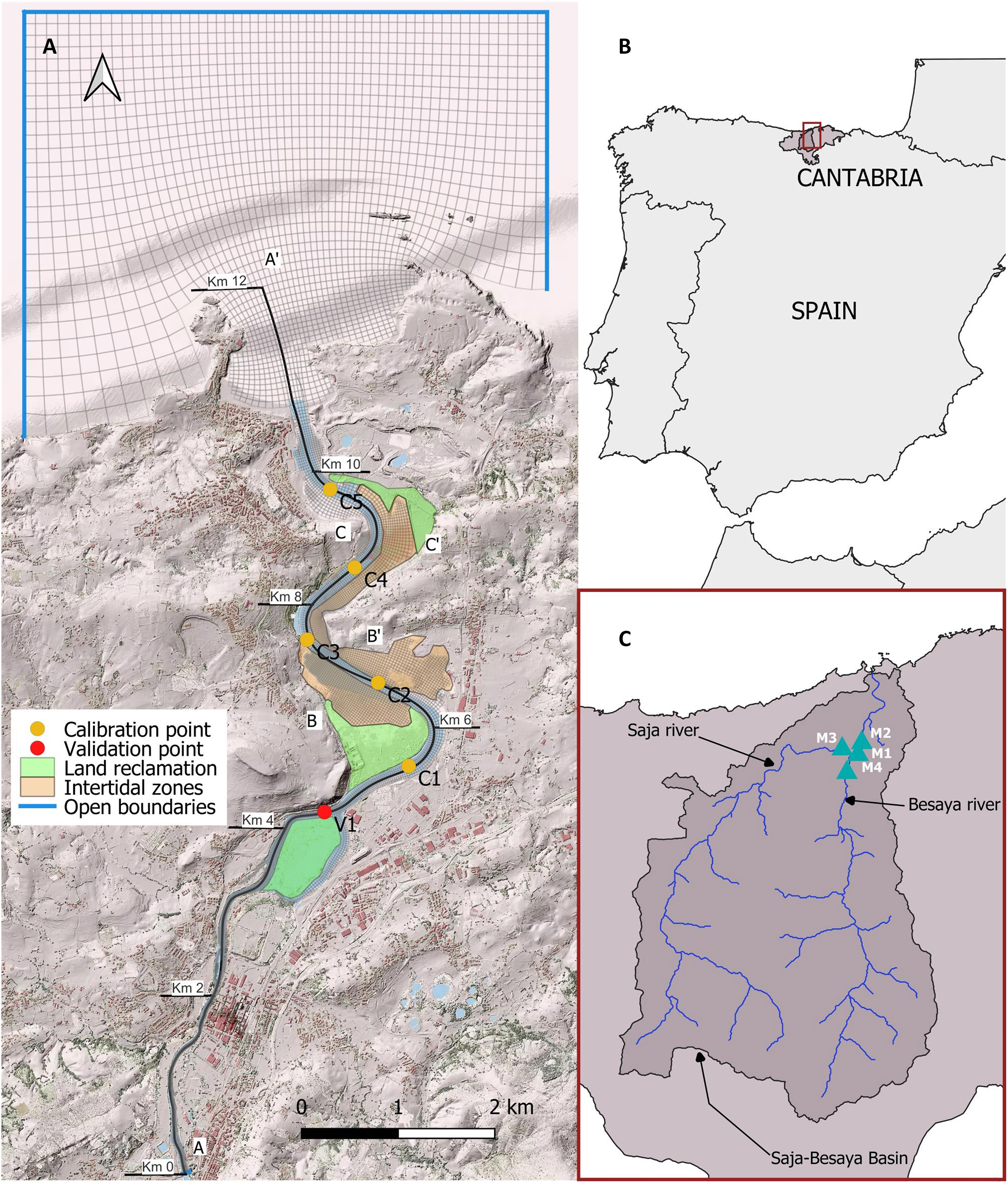
Figure 1 (A) Location of the Suances estuary showing the intertidal zones, the land reclamation zones, the model mesh grid, the model open boundaries, the model calibration points, and the model validation point. The following sections are marked: A-A’ longitudinal section, B-B’ cross-section at intertidal zone 1, and C-C’ cross-section at intertidal zone 2. (B) Location of Cantabria in Spain. (C) Location of the Saja-Besaya river basin in Cantabria showing the meteorological stations used in this study.

In field campaign 1, the used sensors were: (1) 2 acoustic Doppler velocity profiling current meters (ADCPs), Nortek AWAC 1MHz in C3 and C5, (2) 3 Sensus Ultra pressure and temperature sensors. With these devices, 5 points of water levels and temperature (C1 to C5) and 2 points of velocity profiles (C3 and C5) were continuously measured every 10 minutes. Additionally, bottom and surface salinity samples were taken at points C1 and C5 by using a conductivity meter (Hach Intellical CDC401). For this purpose, a scuba diver collected a total of 16 samples (8 at the surface and 8 at the bottom) at the beginning of the campaign during a tidal cycle and another 16 at the end of the campaign.

In field campaign 2, a low-cost support was designed and moored in the estuarine bottom to measure hydrodynamic variables in the water column at different depths. Their location in the Suances estuary was selected based on the findings from Bárcena et al. (2016), being the best place at the survey point V1 (red dot in Figure 1). The sensors were continuously measuring every 15 minutes: (1) 1 ADCP Nortek AWAC 1MHz and (2) 4 Sensus Ultra pressure sensors. The ADCP was moored on the base of the support while the remaining sensors were mounted on the support by means of 3D-printed pieces specifically designed for every sensor.

2.2 Setup of the 3D hydrodynamic model

Delft3D-FLOW software (Lesser et al., 2004) has been used to carry out this study. It consists of a finite-difference-based numerical model that solves shallow water equations in two or three dimensions (Stelling and Leendertse, 1991). These equations are derived from the three-dimensional Navier-Stokes equations for free incompressible surface flow, using the international standard formula of UNESCO (UNESCO, 1981) for density. The Reynolds stress components are computed using the eddy viscosity concept (Rodi, 1987).

Regarding the model setup, a curvilinear grid covering the estuary and its adjacent coastal zone has been implemented (Figure 1) with a vertical distribution of 20 equidistant σ-layers. The open boundaries correspond to the coastal zone and the limit of tidal influence, where tidal (level, temperature, and salinity) and river (flow, temperature, and salinity) forcings have been imposed, respectively. Finally, a heat flow model has been included to calculate the interactions of the atmosphere with the water-free surface fed by the data recorded by the meteorological stations (solar irradiance, air temperature, and relative humidity). For more information about the model setup, readers are referred to Supplementary Material 1. Within this text, further information about how the model has been set up is given. For example how the boundary conditions were defined; the input of initial and boundary conditions; the model parameter settings (viscosity, diffusivity, and bottom roughness); the temporal step used; the grid cell dimension (both horizontal and vertical); how the intertidal regions are solved in the model; or how turbulence is calculated in the horizontal and vertical direction.

Calibration has been focused on adjusting the physical and numerical parameters during the period encompassed by field campaign 1. Physical parameters are the eddy viscosity and diffusivity (horizontal and vertical) and the boundary stresses (bottom, lateral, and surface). Numerical parameters encompass the numerical scheme, the time step, the numerical filters, and the wetting and drying processes. The calibration process has been conducted by comparing the water levels at C1 to C5, the current velocities at C3 and C5, the water bottom temperatures at C1 to C5, and salinity samples at C1 and C5 (see Figure 1). Next, the model has been validated with the information obtained in field campaign 2. In this validation, the physical and numerical parameters have been rechecked by using the data registered at V1 (water levels, current velocities, and temperatures).

Two metric errors have been computed to calibrate and validate the model. First, BIAS is the difference between model results and observed values at the same date, as displayed in Equation 1. Second, the error between both series is calculated using the SKILL parameter developed by Willmott (1981) and defined by Warner et al. (2005) as Equation 2. In this study, the final model configuration was simultaneously displaying the minimum BIAS and the maximum SKILL.

$\begin{array}{ll}BIAS=\sum _i^n\frac{X_{model}-X_{obs}}{N}& (1)\end{array}$

$\begin{array}{ll}SKILL=1-\frac{{\sum }^{}{\left|X_{model}-X_{obs}\right|}^2}{{\sum }^{}{(\left|X_{model}-\overline{X_{obs}}\right|+\left|X_{obs}-\overline{X_{obs}}\right|)}^2}& (2)\end{array}$

where X is the variable being compared, Xobs is the i-datum measured from sampling, Xmodel is the i-datum modeled from simulation, and i is the i-value from 1 to N measurements.

2.3 Methodology to analyze the mixing and stratification alterations in estuaries due to climate change

Figure 2 shows the four steps carried out to develop a methodology for the comparison of the effects of climate change on the mixing and transport in estuaries. The first step has been the model implementation, as seen in section 2.2. Next, subsections 2.3.1 to 2.3.3 will explain the three remaining methodological steps: (1) Selection of climate change scenarios, (2) Climate change predictors, and (3) Analysis of the mixing and stratification alterations in estuaries, respectively.

FIGURE 2

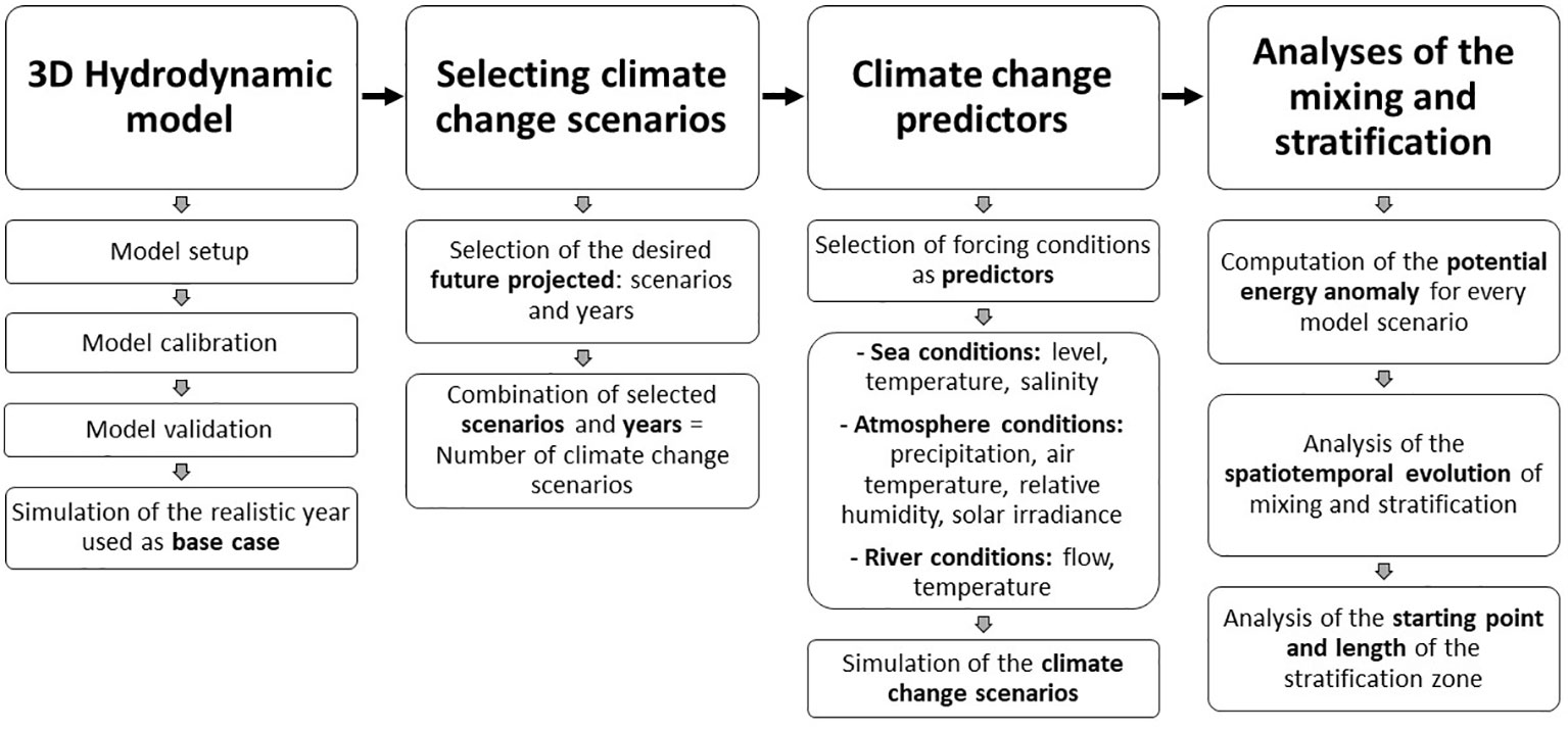
Figure 2 Methodology to analyze the mixing and stratification alterations in estuaries due to climate change.

2.3.1 Selection of climate change scenarios

A fundamental step is the selection of the climate change scenarios in order to forecast and compare the model results. In this case, the most probable ranges of the climate change scenarios RCP 4.5 and RCP 8.5 has been chosen in two projections: 2050 and 2100. Therefore, four cases have been compared with the 2020 base year. Accordingly, the 2020 forcings have been adjusted by using coefficients to adapt them to the projected values in the four study cases.

2.3.2 Climate change predictors

This section identifies the forcings that have been considered in the climate change study as predictors: sea (level, temperature, and salinity), atmosphere (precipitation, air temperature, relative humidity, and solar irradiance), and river (flow and temperature).

In the case of sea predictors, the IPCC and NASA sea level rise forecast viewer, developed by Fox-Kemper et al., 2021, Garner et al., and Garner et al., 2021 has been used to estimate the adjustment coefficients for various scenarios and years of sea level rise. The closest observation point to the study area is called Santander 1. Moreover, the sea temperature has been estimated from the global surface temperature variation collected in the IPCC (2019). Unlike the sea temperature and level, the sea salinity is not a parameter usually analyzed. In the study region, North Atlantic or Cantabrian Sea, changes in salinity are expected to be around 0, either slightly increasing or decreasing (Chust et al., 2010; Durack and Wijffels, 2010; Gomis et al., 2016; Sanz & Galán, 2020; Skliris et al., 2020). Since the projected values are in similar ranges, the values projected by Skliris et al., 2020 have been applied. This study analyzed the changes in the water cycle, giving projections of salinity change in the subpolar region of the North Atlantic (from 40°N to 65°N) up to 2100 for the RCP 4.5 and RCP 8.5 scenarios.

To obtain the atmosphere predictors, the AdapteCCa platform has been used (https://adaptecca.es/). AdapteCCa is a platform for consulting and exchanging information on impacts, vulnerability, and adaptation to climate change (Gutiérrez Llorente et al., 2018). The platform viewer provides forecasts for many variables made by a model ensemble up to the year 2100, including precipitation and temperature. In the study region, Torrelavega ‘SNIACE’ -1131l (see M1 in Figure 1) has been selected as the reference station for the forecast. First, daily data with precipitation and temperature forecasts for RCP 4.5 and RCP 8.5 have been downloaded. Next, the average value of all models has been chosen for precipitation while, for temperatures, the available data are the maximum and minimum temperatures, so the average between them has been made. To analyze the changes in the different scenarios, the monthly percentage changes of each parameter have been established, so that monthly variation coefficients could be obtained for the projections in 2050 and 2100 of the RCP 4.5 and RCP 8.5 scenarios. For this purpose, the results of the two scenarios in 2020 have also been downloaded from the application to obtain the variations from the same data source. With these adjustment coefficients, the precipitation and temperature of M1 have been projected. Accordingly, a realistic rainfall of the year 2020 can be projected. The advantage of this methodology is that since it does not modify rainfall patterns, just their projected intensity, we can compare the different projections and evaluate the effects of climate change on a common baseline situation. Lastly, the relative humidity and solar irradiance have been kept because there are no data for their evaluation forecasts, so it will be considered that their conditions will not change in the projection of climate scenarios.

For the river predictors, precipitation and air temperature estimations have been used as input for the hydrological model in order to obtain new river flows. Additionally, the river temperature has been established by applying the same relationship between river temperature and air temperature used for the model calibration and validation to the projected air temperature data.

2.3.3 Analysis of the mixing and stratification alterations in estuaries

PEA have been used to identify the mixing and stratification alterations in the estuary, PEA is defined in Equation 3 as the amount of mechanical energy (per m³) necessary to instantaneously homogenize the water column with a given density, i.e., the average density of the water column.

$\begin{array}{ll}PEA=\frac{1}{H}\underset{-h}{\overset{\eta }{\int }}gz(\overline{\rho }-\rho )dz=-\frac{1}{H}\underset{-h}{\overset{\eta }{\int }}gz\widetilde{\rho }dz & (3)\end{array}$

$\begin{array}{ll}\widetilde{\rho }=\rho -\overline{\rho }& (3)\end{array}$

where $\rho$ is the vertical profile of densities over the water column H; H is the total height of the water from the bottom (-h) to $\eta$; $\eta$ is the vertical coordinate of the water surface at a given instant; $z$ is the vertical coordinate; $g$ is the acceleration of gravity; $\overline{\rho }$ is the mean density of the water column and $\widetilde{\rho }$ is the density fluctuation in the water column. It should be noted that the higher the PEA, the higher the stratification.

Next, the starting point and length of the stratification zone have been hourly calculated for the thalweg of the estuary (A-A’ section in Figure 1; Figure S9) for every scenario. The starting and the end points of the stratification zone are the first and last grid cells of A-A’ section where PEA is higher than 2 J/m³, respectively. Finally, the length of the stratification zone has been computed as the difference between the end and starting point distances from the beginning of the A-A’ section.

3 Results

3.1 Model calibration and validation in the Suances estuary

Tables 1, 2 show the magnitude of the metric errors (BIAS and SKILL) calculated at all the locations for model calibration and validation, respectively. Note that these magnitudes have been obtained by comparing every fifteen-minute the data recorded in the field campaigns and computed by the model.

TABLE 1

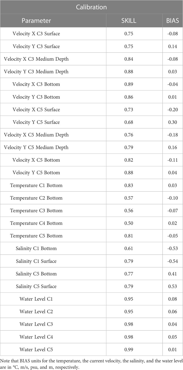
Table 1 SKILL and BIAS results for the model calibration.

TABLE 2

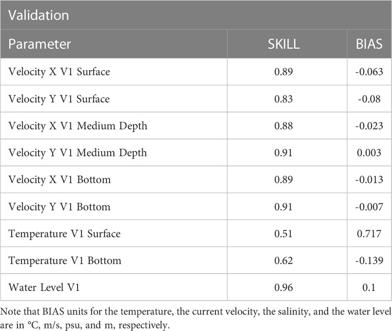
Table 2 SKILL and BIAS results for the model validation.

As displayed in Tables 1, 2, the water levels are excellently reproduced, with SKILL values higher than 0.95 in any case and BIAS values around 0. This is because very tight data has been obtained for the incoming forcings, since a detailed study was carried out to determine which incoming forcings gave the best accuracy to the model. The velocity is well reproduced, with SKILL values from 0.67 to 0.89 on the surface to values from 0.78 to 0.91 at the middle and the bottom depths. BIAS values are displaying an average of 0.11 m/s. This difference between bottom and surface values can be explained by the wind effect, which is not being taken into account in the calculations. Although wind is not a significant forcing in the Suances estuary due to its surface area is low, wind can cause small variations in the surface measurements. On the other hand, velocities at middle and bottom depths are reproduced with very good resolution because a new bathymetry was performed in this area. In addition, it should be noted that the velocities have lower SKILL and BIAS values than other parameters due to turbulence (instantaneous velocities).

The salinity adjustments are around a SKILL of 0.6 to 0.8, so it is considered a good fit while BIAS is between -0.5 and 0.5 psu (very good fit). Finally, the temperature varies in a SKILL of 0.5 to 0.8. This variability is mainly because the sensor has not properly registered the tidal changes. Furthermore, the river temperature has been imposed by using Equation S1 and Equation S2, as shown in Supplementary Material 1. These relationships take the air temperature as the predictor, so small temperature variations at each time step have been induced in the river temperature that could be slower in reality. Nevertheless, BIAS settings are very good, with an average value around 0 and 0.4 C° for the calibration and validation, respectively. Readers interested in a detailed explanation of the model calibration and validation are referred to in Supplementary Material 1.

3.2 Climate change predictors

To carry out the climate change projections, the 3D hydrodynamic model with the forcings for the year 2020 has been used as a baseline scenario. The forcings that have been considered in the climate change study as predictors in the 3D hydrodynamic model are related to sea (level, temperature, and salinity), atmosphere (precipitation, air temperature, relative humidity, and solar irradiance), and river (flow and temperature).

Table 3 collects the applied changes to the climate change predictors of sea conditions: level, temperature, and salinity for the projected climate change scenarios: 2050 RCP 4.5, 2100 RCP 4.5, 2050 RCP 8.5, and 2100 RCP 8.5. In addition, Table 4 presents the expected monthly changes in the climate change predictors of atmospheric conditions: precipitation and air temperature for the projected climate change scenarios: 2050 RCP 4.5, 2100 RCP 4.5, 2050 RCP 8.5, and 2100 RCP 8.5. Finally, it is noteworthy to mention that (1) the river temperature has been indirectly established by applying the relationship between river temperature and air temperature; and (2) the relative humidity and solar irradiance have been kept the same as the year 2020.

TABLE 3

Table 3 Applied changes to sea level, sea surface temperature, and sea salinity for the projected climate change scenarios relative to the 2020 year: 2050 RCP 4.5, 2100 RCP 4.5, 2050 RCP 8.5, and 2100 RCP 8.5.

TABLE 4

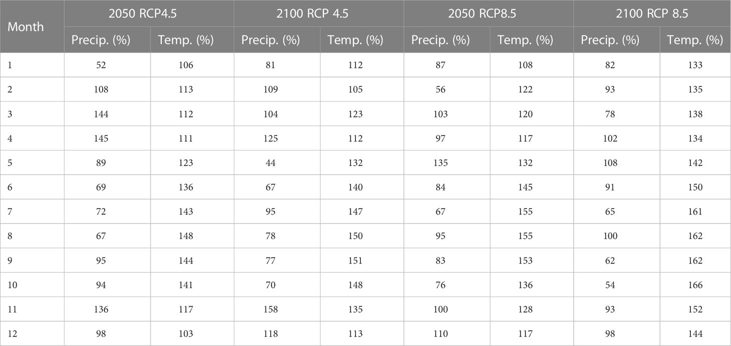
Table 4 Expected monthly changes in precipitation and air temperature for the projected climate change scenarios relative to the 2020 year: 2050 RCP 4.5, 2100 RCP 4.5, 2050 RCP 8.5, and 2100 RCP 8.5.

Figure 3 displays the sea level (A), the sea salinity (B), the sea temperature (C), the precipitation (D), the air temperature (E) the river flow (F), and the surface river temperature (G) included in the 3D hydrodynamic model for every selected scenario (2020 - black solid lines, 2050 RCP 4.5 – red solid lines, 2050 RCP 8.5 – blue solid lines, 2100 RCP 4.5 – red dashed lines, and 2100 RCP 8.5 – blue dashed lines).

FIGURE 3

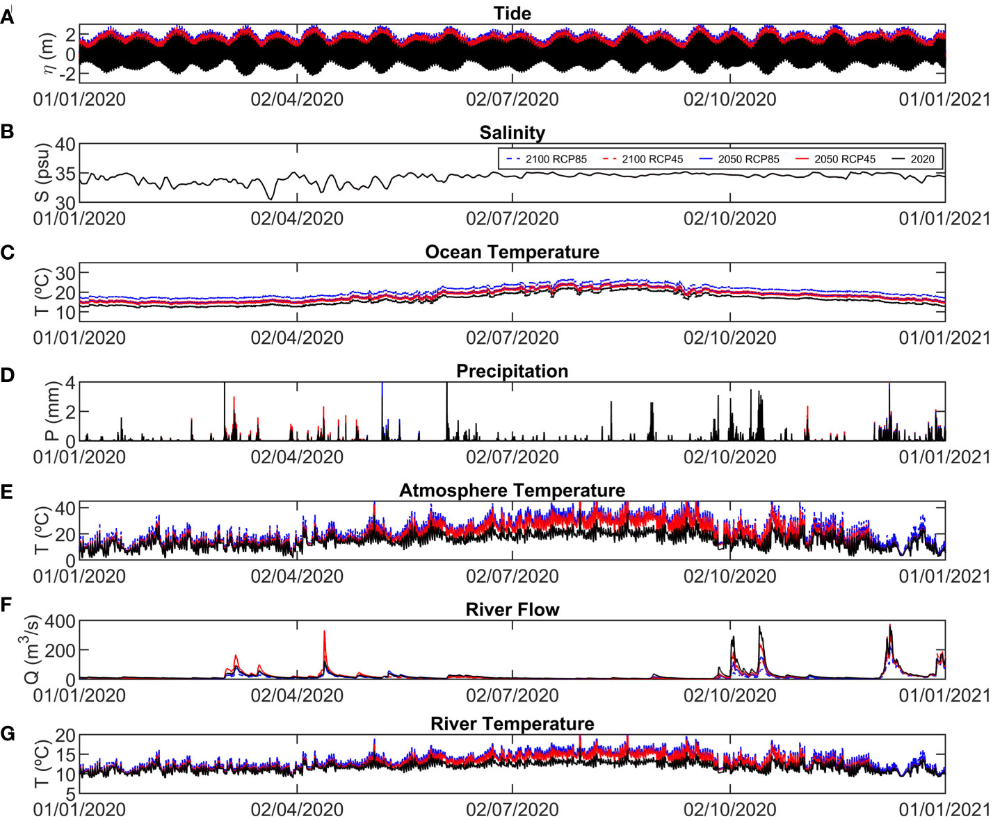
Figure 3 Forcings applied to the different climate change scenarios. (A) Sea level, (B) sea salinity, (C) sea temperature, (D) precipitation, (E) air temperature, (F) river flow, and (G) surface river temperature.

Analyzing the sea level (see Table 3; Figure 3A), a progressive rise according to the analyzed year and scenario is displayed, which is in line with all IPCC reports and scientific studies, ranging from 0.25 to 0.82 m. Regarding the sea temperature (see Table 3 and Figure 3E), an exponential increase is foreseen for the year 2100, ranging from 1.7 to 4.3 °C. Although these values are high, especially for RCP 8.5 and the 2100 scenario, it is important to mention that these values have been found in other studies for the short term (2031-2050) and the end of the century (2080-2100) (IPCC, 2019). Concerning the sea salinity (see Table 3; Figure 3D), a slight decrease of -0.004 psu is experimented by 2050 in any RCP, while for the year 2100 a slight increase is expected, ranging from 0.003 to 0.011 psu.

As can be seen in Table 4; Figure 3F, there is a clear increase in air temperature, around 50% on average in the coming years according to the scenario analyzed. These results, obtained from https://adaptecca.es/, show a globalized increase in atmospheric temperature as reported by IPCC, 2021. In addition, the greatest temperature changes will occur between the months of July and October. The average of the annual changes shows an increase of 126% for the year 2050 and RCP 4.5, 132% for the year 2100 and RCP 4.5, 135% for the year 2050 and RCP 8.5 and the highest, 150% for the year 2100 and RCP 8.5. Regarding the precipitation (see Table 4; Figure 3A), there is a significant variation, with a tendency to decrease, especially in the year 2100. In the short term (the year 2050), there is a distribution of precipitation that causes a decrease in precipitation in the central months of the year and an increase in precipitation in the winter months associated with extreme precipitation events compared to the year 2020. This interannual variability is reduced in the year 2100, predicting a more generalized reduction in precipitation compared to the year 2020. In the long term, there is a tendency to decrease in precipitation oriented towards the forecasts of desertification of the Iberian Peninsula (IPCC, 2021). As for the average annual variations, these do not significantly vary from the 2020 base series, obtaining a variation of 102% for the year 2050 and RCP 4.5 scenario, 95% for the year 2100 and RCP 4.5 scenario, 91% for the year 2050 and RCP 8.5 scenario and, finally, 86% for the year 2100 and RCP 8.5 scenario.

In the case of river flow (see Figure 3B), significant variations can be observed due to the changes in precipitation and air temperature. Except in specific cases, the flow trend tends to decrease compared to the base year 2020, mainly due to the increase in air temperatures that causes less snowfall, together with a general decrease in precipitation as shown in Table 4.

3.3 Spatiotemporal evolution of mixing and stratification in the Suances estuary due to climate change

In this section, an analysis of the annual variability in the Suances estuary has been carried out in order to relate the main estuarine forcings (tide and river flow - Figures 4A, B) to the spatiotemporal evolution of PEA. Figure 4C shows the Hovmöller diagram (Hovmöller, 1949) for the PEA values during the 2020 year along the estuarine longitudinal section (see A-A’ section in Figure 1). Analogously Figures 4D, E show the Hovmöller diagram for the PEA values during the 2020 year along two estuarine transversal sections, located at the intertidal zone 1 (see B-B’ section in Figure 1) and the intertidal zone 2 (see C-C’ section in Figure 1). Readers interested in the geometry and bathymetry of these sections are referred to Supplementary Material 1 (Figure S9).

FIGURE 4

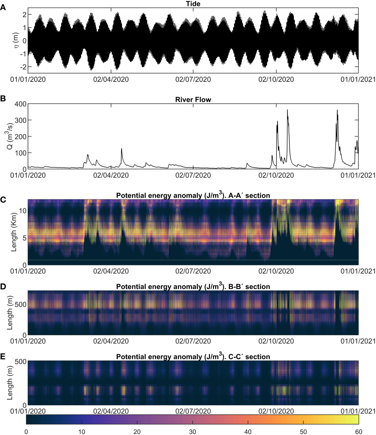
Figure 4 (A) Sea level and (B) River flow for the year 2020. Hovmöller diagram of the year 2020 with hourly PEA values along the estuarine sections: (C) A-A’ section, (D) B-B’ section, and (E) C-C’ section.

As shown in Figure 4, there is a significant influence of the river discharge on the location of the stratification zone along the A-A’ section, as indicated by the black spikes in the PEA that correlate with the discharge spikes in the plot above. During low flows (0 to 10 m³/s), the zone of highest stratification, denoted by the yellow color, which shows the highest PEA values, is located between km 4 and 8 with the maximum value oscillating by the alternate of spring and neap tides. The maximum values of PEA in this zone vary from 10 to 50 J/m³ depending on the ebb-flood cycle. At the estuarine mouth, PEA values are very low during spring tides, nearly 0; increasing their magnitude as the tide evolves to neap tides, rising up to 20 J/m³. On the other hand, during high-flow events (>100 m³/s), the stratification zone moves towards the mouth as much as the river flow magnitude, displaying values of up to 200 J/m³ during spring tides. In these cases, areas with very low PEA values are observed in the estuarine head, because the fluvial discharge flushes all saline water from this zone.

Regarding the transversal sections, the main stratification is centered at the main channel, where the PEA values are the highest (yellow shadows). Along B-B’ section, the river flow has a significant influence at intermediate flows (10 to 100 m³/s), generating the highest stratification, up to 50 J/m³. On the contrary, at high flows, B-B’ section becomes fully mixed. Along C-C’ section, these phenomena are not so noticeable. Although PEA values are also higher in the main channel than in the intertidal zone, the occurrence of a stratification zone is less frequent over time (up to 57% lower). It is also noteworthy that in C-C’ section, there is no full mixing during high and intermediate flows (values from 2 to 21 J/m³). This is due to its proximity to the estuarine mouth, which means that, during these events, the stratification zone is centered in this area. However, at low flows, all the C-C’ section is mixed due to the tidal effect (PEA values below 2 J/m³).

Figures 5, 6 show the differences observed in PEA values by subtracting the 2020 baseline scenario from the projected climate change scenarios (Panels a - 2050 RCP4.5, Panels b - 2050 RCP8.5, Panels c - 2100 RCP4.5, and Panels d - 2100 RCP8.5) at A-A’ section (see Figure 5), B-B’ section (see Figure 6), and C-C’ section (see Figure 6). In both figures, note that the positive and negative variations of PEA, as well as the intensity of the changes, can be located.

FIGURE 5

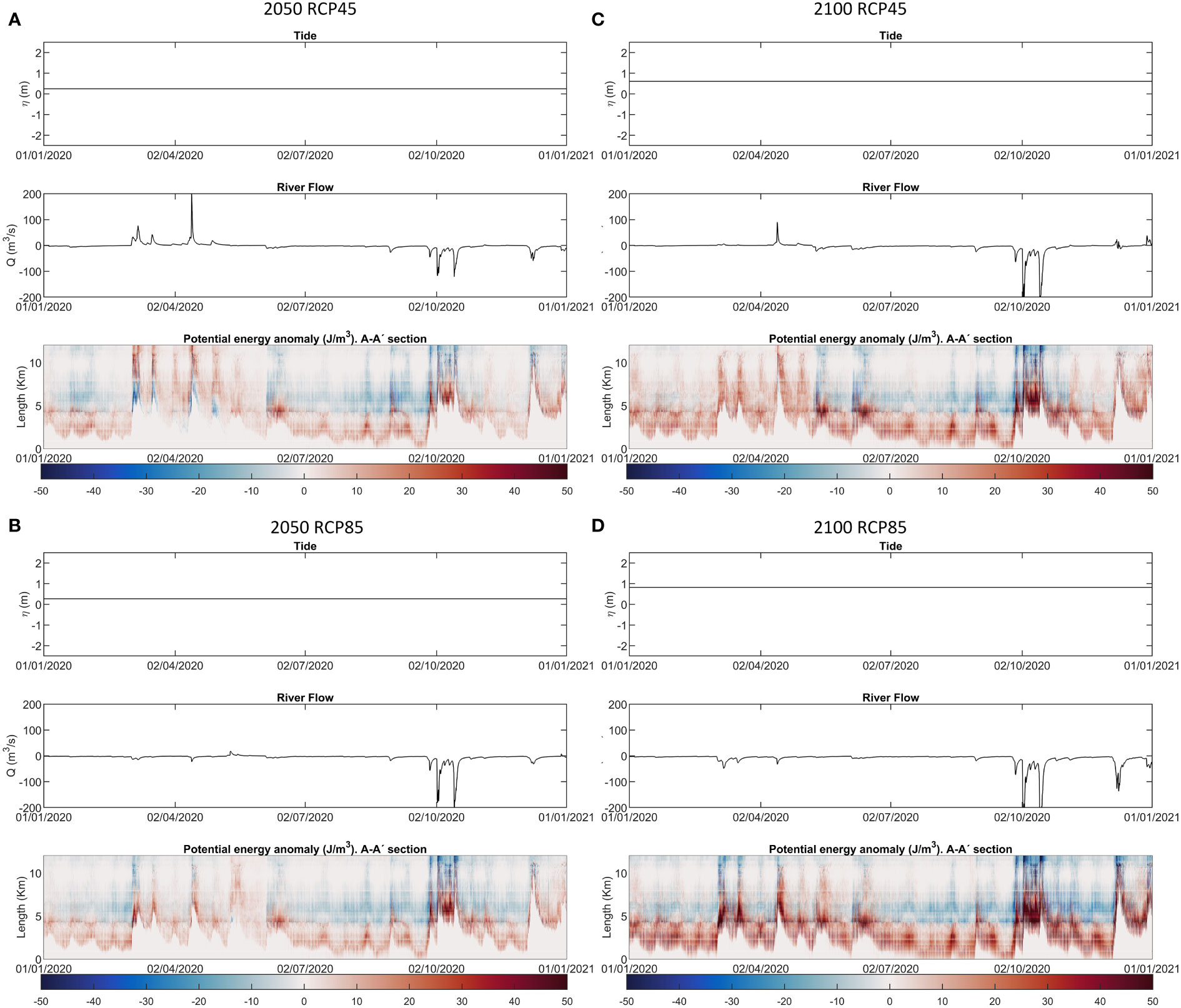
Figure 5 Expected changes in forcings: sea level (upper panels) and river flow (middle panels). Hovmöller diagram of the differences observed in PEA values by subtracting the 2020 baseline scenario from the projected climate change scenarios (A) - 2050 RCP4.5, (B) - 2050 RCP8.5, (C) - 2100 RCP4.5, and (D) - 2100 RCP8.5) at A-A’ section (lower panels).

FIGURE 6

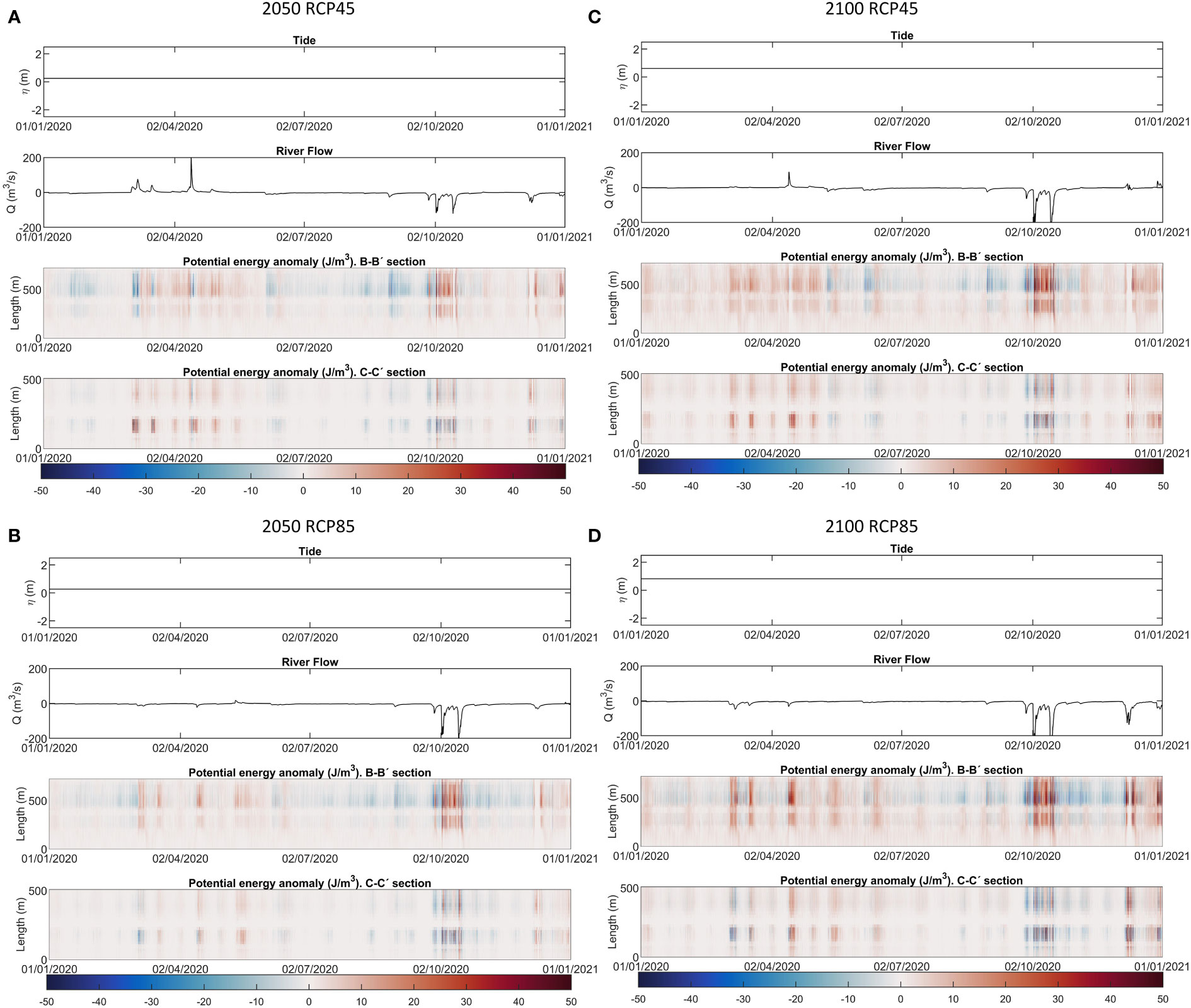
Figure 6 Expected changes in forcings: sea level (upper panels) and river flow (middle panels). Hovmöller diagram of the differences observed in PEA values by subtracting the 2020 baseline scenario from the projected climate change scenarios (A) - 2050 RCP4.5, (B) - 2050 RCP8.5, (C) - 2100 RCP4.5, and (D) - 2100 RCP8.5) at B-B’ section (low panels) and C-C’ section (lower panels).

Depending on geometric and bathymetric features, there are spatially differentiated zones within an estuary (Bárcena et al., 2012b), which, in turn, could modify the mixing and stratification at different zones of the estuary for the same system’s forcers. Accordingly, the Suances estuary has been divided into 16 independent boxes and one additional box 17 (box 17), which is the sum of all the previous boxes (Figure 7). The division of the boxes has been made based on geometric features: (1) the curve and straight zones of the main channel, and (2) the dykes that separate the intertidal zones from the main channel. The main channel has been divided into the upper zone (boxes 1, 2, and 3), the middle zone (boxes 4, 5, 6, and 7), and the lower zone (boxes 8, 9, and 10). Boxes from 11 to 16 comprise the estuarine intertidal zones. Finally, Figure 7A collects the hourly PEA mean value (J/m³) of each box and the expected changes (%) relative to the 2020 year for the climate change scenarios and the location of the divided boxes in the Suances estuary (Figure 7B). To obtain the PEA values in Figure 7A, firstly, PEA has been calculated for every time step (1 hour) and grid cell of each box (Figure 7B). Secondly, PEA of each box has been spatiotemporally averaged by the elapsed time of each Scenario and the grid cell size.

FIGURE 7

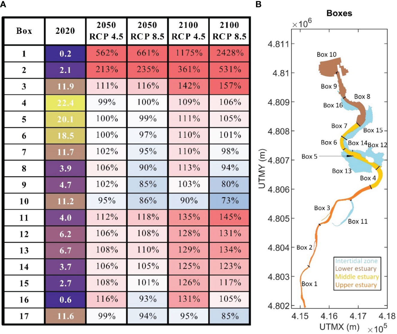
Figure 7 A) Hourly PEA mean value (J/m3) of each box and the expected changes (%) relative to 2020 for the projected climate change scenarios, and B) the location of the divided boxes, being box 17 the Suances estuary.

Figure 5 shows the differences in the flow rates for every scenario. The river flow tends to decrease except at the beginning of the year in the 2050 RCP 4.5 scenario. These changes in flow are quantitatively small in most cases, since at low flows (0 to 10 m³/s) the magnitude to reduce flows is small. However, a potential decrease in flow rates of around 2-5 m³/s can be observed for all scenarios. On the other hand, when analyzing high flow events (more than 100 m³/s), the differences between the flow rates are higher, with potential reductions of up to 300 m³/s of instantaneous flow in the RCP 8.5 scenario for the year 2100, and reductions varying from 150 to 250 m³/s in the rest of the scenarios. In terms of average annual values, the estimated average flow in 2020 was 29 m³/s. Comparing the average values of the projected scenarios, a decrease in flow of 86% and 85% for the RCP 4.5 scenarios and 77% and 61% for the RCP 8.5 scenarios are observed for the years 2050 and 2100, respectively.

As displayed in Figure 5, independently of the climate change scenario, the stratification intensity increases and decreases upstream and downstream of the estuary, respectively. These results indicate that the stratification zone will move upstream of the estuary. Unlike the 2020 base scenario, in which the stratification zone has been mainly centered between km 4 and 8, for the new climate change scenarios, the stratification zone will be displaced between km 2 and 8, attenuating its intensity from km 4 onwards. During extreme events, the areas of maximum stratification will occur in the middle zone of the estuary, unlike the current dynamics that placed it in the outer zone. Moreover, the stratification intensity proportionally increases and decreases in the inner and outer zones, respectively. In the 2020 scenario, average PEA values range from 0.2 J/m³ in the upper part of the estuary to 22.4 J/m³ into box 4 (Figure 7). In the 2020 scenario, the zone of maximum stratification is centered in boxes 4, 5, and 6, which corresponds to the middle part of the estuary, with lower mean values in the upper and lower sections. When comparing the variations, it is observed that the mean values of PEA clearly increase in the upper estuary boxes and decrease in the lower estuary. As shown in Figure 5, the stratification moves upstream, with very significant increases of more than 200% in boxes 1 and 2. On the other hand, in the intermediate zone, boxes 4, 5, and 6, there are hardly any differences in the mean PEA values, being in the same range as in the 2020 comparison year. Finally, it is noteworthy how a decrease in PEA is observed in the upper boxes (8, 9, and 10), which corresponds, as seen in Figure 5, with a zone of full mixing due to the tidal. At boxes 8, 9, and 10, decreases of up to 25% are observed in the most unfavorable case (2100 RCP 8.5).

As can be seen in Figure 6, the obtained results in the cross sections are similar to the longitudinal section. The B-B’ section, which corresponds with boxes 5, 12, and 13 from Figure 7B, tends to have higher positive values during high flows as opposed to C-C’ section, which corresponds with boxes 8 and 15 from Figure 7B, which tends to be negative due to the displacement of the stratification zone. On the other hand, during intermediate and low flows, the stratification intensity increases and decreases in equal parts. As for the differences between the main channel and the intertidal zone, the main channel maintains higher PEA values than the intertidal areas, as shown in Figure 7, pointing out that the main channel is more vulnerable to changes than the intertidal zones. However, the increase of intensity in the intertidal zones compared to the 2020 base scenario indicates that the intertidal zones will be more stratified in the projected climate change scenarios. In Figure 7, all the intertidal zones increase the PEA values, evidencing the generalized increase in stratification, more marked in boxes 12 and 13 than in 15, as shown in Figure 6. These variations change in each scenario, reaching increases of more than 130%. This trend is originated by the sea level rise because the intertidal zones tend to similarly behave to the main channel because of the increase in the water column depth. However, it is important to consider that this assumption is made without considering the potential bathymetric changes produced by sediment input/withdrawal that may occur over the years.

As shown in Figure 7, there is an increase in the mean values of PEA in the upper part of the estuary, mainly induced by the increase in sea level and the decrease in flow. Analyzing the annual mean values for the Suances estuary, it can be seen how for the base year 2020 the weighted mean value reached 11.6 J/m3. In the subsequent scenarios, a generalized decrease in this average value can be seen, which can decrease up to 15% in the 2100 RCP 8.5 scenario. Analyzing the different parts of the estuary, a generalized increase of PEA is observed in the upper boxes. In this zone, values of up to 2000% relative to the base year 2020 are reached, which intensifies as years and scenarios progress. In the middle part of the estuary, however, PEA values are maintained or increased by a maximum of 13% depending on the scenario analyzed, showing that this zone remains practically unchanged. Finally, in the lower part of the estuary, PEA values tend to decrease in a generalized pattern, up to 15% because of the mixing produced in these areas by seawater intrusion from sea level rise. Finally, in the intertidal zones, there are generalized increases in the stratification zones, reaching values from 101% to 145% compared to the base year 2020.

4 Discussion

The Suances estuary presents and will present under the considered scenarios a high spatiotemporal variability of the mixing and stratification processes. Due to climate change, the stratification zone will be modified as observed in other estuaries worldwide (Leal Filho et al., 2022; Costa et al., 2023). On the one hand, sea level rise will pull the stratification zones back inland from the estuary as seen in the various studies analyzed in the region surrounding the study area, such as the NW Atlantic coast of Portugal (Pereira et al., 2022) or the UK coast (Robins et al., 2016). On the other hand, climate change will generate lower precipitations and higher temperatures, decreasing runoff events similar to studies analyzed in the Mediterranean (Hallett et al., 2018) or the Atlantic (Robins et al., 2016) climate zones. This phenomenon will decrease the freshwater input to the estuary and increase the tidal excursion along the estuary, producing a displacement of the river/estuarine front upstream in line with the results observed by Ma et al., 2023.

Figure 8 shows the empirical cumulative distribution function (ECDF) curves of the starting point A and the length of the stratification zone B for every climate change scenario: 2020 (black solid line); 2050 RCP 4.5 (red solid line); 2050 RCP 8.5 (blue solid line); 2100 RCP 4.5 (red dashed line); and 2100 RCP 8.5 (blue dashed line).

FIGURE 8

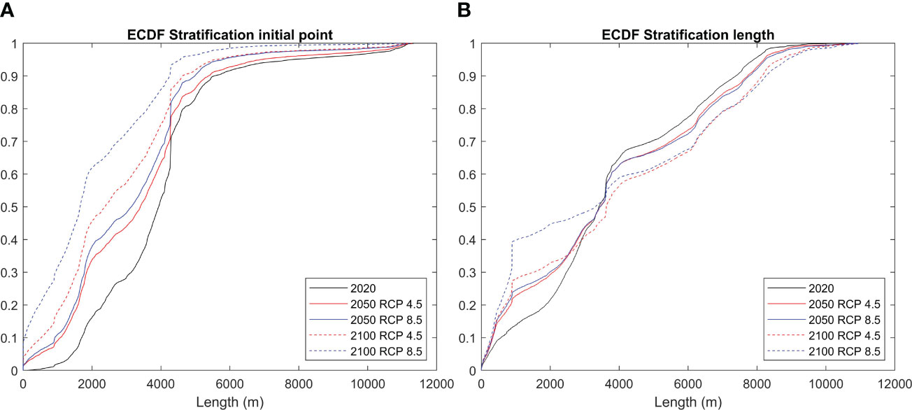
Figure 8 Empirical cumulative distribution function for the starting point (A) and length (B) of the stratification zone for every climate change scenario: 2020 (black solid line); 2050 RCP 4.5 (red solid line); 2050 RCP 8.5 (blue solid line); 2100 RCP 4.5 (red dashed line); and 2100 RCP 8.5 (blue dashed line).

As shown in Figure 8, the starting point of the stratification zone moves upstream of the estuary in the projected scenarios as seen in the Minho estuary in Pereira et al., 2022 and the Wu river in Liu and Liu, 2014, where salinity intrusion extends more than 2.000 m and 900 m in the projected scenarios, respectively. In the Minho and Wu estuaries, sea level rise is the main cause of increased salinity intrusion. However, in other cases, river flow may govern the starting point, as shown by Yang et al., 2015 in the Snohomish River estuary. On the other hand, in the year 2020, the most probable stratification zone starts at km 4, where the cumulative probability rises almost vertically. However, this trend is altered in the projected climate change scenarios, since the verticality previously shown is reduced and displaced. In projected climate change scenarios, the most probable starting point is concentrated on two zones. For the 2050s scenarios, the most probable starting point is located above km 2 or km 4. As for the year 2100, a uniform probability can be observed from km 1 to km 2, after which it loses that verticality. Regarding the length of the stratification zone, its variability is smaller than the starting point. In the Suances estuary, the length of the stratification zone will be reduced up to a length of 4 kms and extended beyond that length. The river flow will have a significant influence, because the higher the flow, the shorter the length of the stratification zone. Additionally, the longest lengths occur at flood tides and low flows because these forcing conditions favor the stratification over the mixing processes by reducing the estuarine kinetic energy and, subsequently, the available turbulence for mixing.

Table 5 collects the response surfaces regressed from the dataset of 8785 model outputs (hourly data for the year 2020 for the location of the starting point of the stratification zone and its length, based on the river flow (Q) and the water level (N) at the head and mouth of the Suances estuary, respectively. The approximating function used to generate the response surface takes a quadratic form (Equation 5). The data used to perform these regressions are shown in Supplementary Material 1 (Figures S10, S11).

TABLE 5

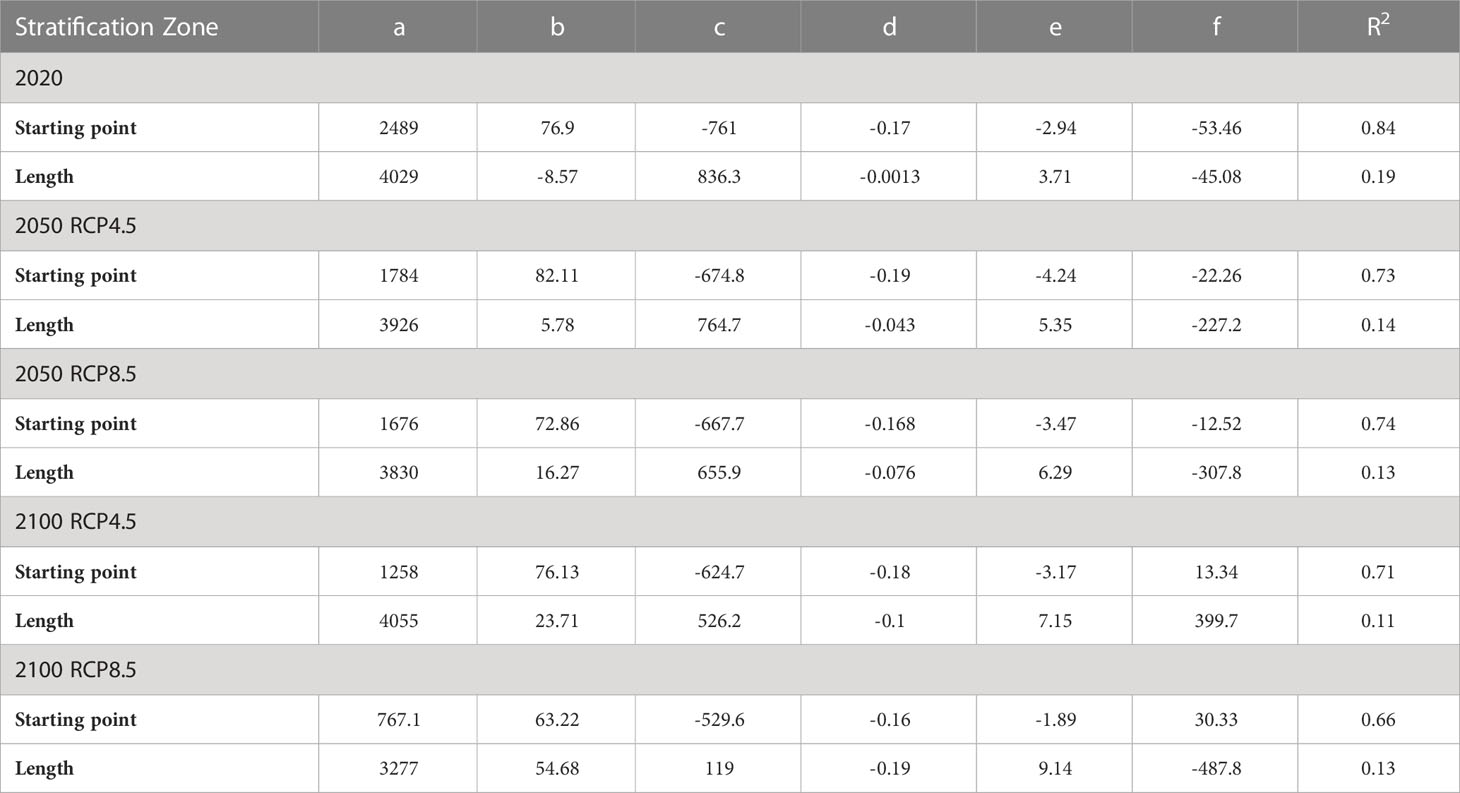
Table 5 Coefficients of the surface fitting functions (A–F) and the regression coefficients (R²) in the Suances estuary for the location of the starting point of the stratification zone from the river boundary and the length of this zone.

$\begin{array}{ll}z=a+bQ+cN+d{Q}^2+eQN+f{N}^2& (5)\end{array}$

As displayed in Table 5, the starting point of the stratification zone is determined with reasonable accuracy, based on two inputs, the river flow and the water level at the estuarine mouth. Unlike the correlations performed by Yang et al., 2015, in this case, the introduction of the water level term is of vital importance, as it modulates the starting and length of the mixing zone. On the other hand, the length of the stratification zone is difficult to estimate accurately, since it is highly dependent on the tidal cycles. Therefore, the distribution of the stratification zone in the Suances estuary fundamentally varies as a function of river flow and sea level similar to that found in Costa et al. (2023) or Robins et al. (2016).

In the Suances estuary, the mixing is actively dynamic and occurs along its entire length, with more mixing at certain locations. Figure 9 shows the residual velocity (black arrows) and density profiles at the longitudinal section (see A-A’ section in Figure 1) for the year 2020 (Figure 9A), and the differences in the residual velocity and density between the 2020 base year and the projected scenarios: 2050 RCP 4.5 (Figure 9B), 2050 RCP 8.5 (Figure 9C), 2100 RCP 4.5 (Figure 9D), and 2100 RCP 8.5 (Figure 9E).

FIGURE 9

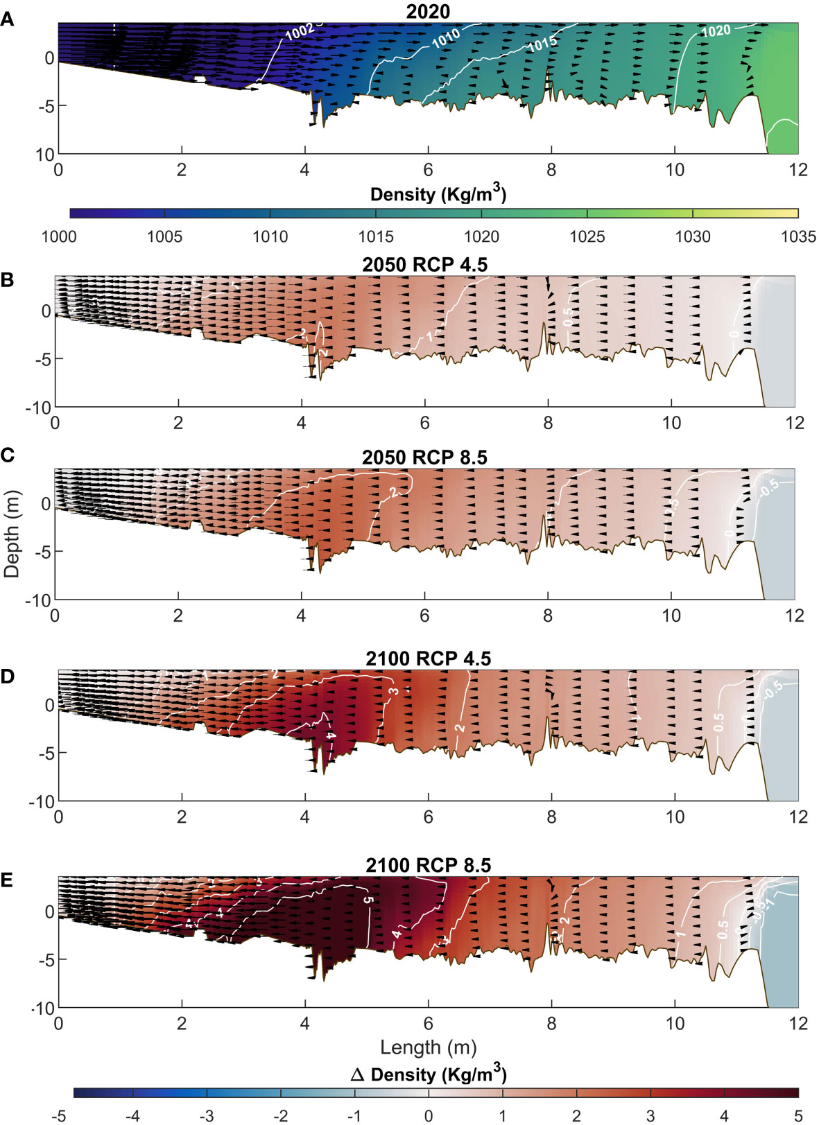
Figure 9 (A) Residual velocity (black arrows) and density profiles (white lines are the isodensity contours of 1002, 1005, 1010, 1015, 1020, and 1025 kg/m³) at the longitudinal section (A-A’ section) for the year 2020. Differences in the residual velocity and density profiles (white lines are the isodensity contours from -5 to 5 kg/m³) between the 2020 base year and the projected scenarios: (B) 2050 RCP 4.5, (C) 2050 RCP 8.5, (D) 2100 RCP 4.5, and E) 2100 RCP 8.5.

Mixing and stratification in the Suances estuary are strongly modulated by tidal cycles, especially at low flows. However, at high flows, the tide takes second place since the inflow of a large amount of freshwater flushes the stratification zone to the estuarine mouth. However, analyzing the annual averages of densities and velocities of the year 2020, the residual current tends to flow out towards the estuary, mainly due to the asymmetry of the tide and the river flow. On the other hand, it can be observed how the density generates gradients that originate small stratifications in the estuary, located between km 4 and 8. Nevertheless, in the projected climate change scenarios, a density increase is observed at the middle and lower parts of the estuary, from 1 to 5 kg/m³. Furthermore, the residual velocities may tend towards a higher intrusion.

These results are in line with the results found by Liu and Liu, 2014; Duvall et al., 2022; Pereira et al., 2022 and Costa et al., 2023, where the increase of salinity intrusion in the estuaries is reported due to sea level rise. It is important to point out that the salinity and density in the Suances estuary are strongly related and the changes in temperature will be minimal as shown in Table 3. These changes in the mixing and stratification of the water column condition the salinity intrusion, affecting the wildlife residing in the estuary (Hallett et al., 2018) and the activities taking place around these ecosystems (Weatherdon et al., 2016).

Finally, it is necessary to address that the studies presented in this work have certain assumptions and limitations, so it is necessary to take the results obtained with caution. On the one hand, variability in physical forcing mechanisms is a large source of uncertainty regarding future changes in density stratification (Duvall et al., 2022). On the other hand, the morphological evolution of the estuary has not been considered, which due to sediment input/withdrawal over the years could modify the estuarine bathymetry, and consequently, could alter the mixing and stratification patterns observed in this study. Finally, it should be noted that the model has been used to examine four specific climate change scenarios. These are not real and should not be treated as such. They represent narratives of what might happen and any modeling that uses them is similarly just examining the possible outcomes of a particular narrative (scenario).

5 Conclusions

A high-resolution 3D hydrodynamic model has been implemented, calibrated, and validated in the Suances estuary, offering a high level of detail and reliability about the estuarine circulation. First, the year 2020 has been modeled using the following forcings: sea (level, temperature, and salinity), atmosphere (precipitation, air temperature, relative humidity, and solar irradiance), and river (flow and temperature). Based on the 2020 forcings conditions, their time series have been adapted to the climate change forecasts for the years 2050 and 2100, taking into account the RCP 4.5 and RCP 8.5 scenarios. Next, the four climate change scenarios have been modeled to analyze the alterations in the competition between mixing and stratification in the water column by means of the calculation of the Potential Energy Anomaly (PEA).

The Suances estuary presents a high spatiotemporal variability in its vertical structure, with the tide playing a leading role in modulating the overall fluctuations. Most of the time, the stratification zone is located between km 4 and 8, varying according to the flood and ebb tides. However, during high-flow river events, the tide plays a secondary role since the fluvial input moves the estuarine water toward the estuarine mouth. Accordingly, the influence of the river is extremely important in the estuary since the higher the flow, the shorter the length of the stratification zone, and the larger the displacement of the stratification zone towards the outside of the estuary.

Regarding the changes in climate change predictors, an increase in air temperatures and a decrease in precipitation is expected in the study area. For the scenarios modeled, extreme fluvial events are more significant in the 2050 scenarios, whereas in the 2100 scenarios a reduction in fluvial flows will reduce the estuarine buoyancy input. For sea conditions, the sea level rise and, to a lower degree, the density changes in the water flows (due to the increase in water temperature and the salinity changes) can be directly related to the displacement of the stratification zone upstream of the estuary. This phenomenon, aided by the decrease in river flows, facilitates the entry of seawater into the estuary, i.e., the saline intrusion is larger with the associated stress this could cause to local ecosystems. Moreover, this effect will tend to increase the intensity of stratification upstream of the estuary and decrease downstream as time and climate scenarios progress.

Data availability statement

The raw data supporting the conclusions of this article will be made available by the authors, without undue reservation.

Author contributions

JL participated in the design of the study, collected the data, performed the data analysis and the hydrodynamic modeling, and drafted the manuscript. JB conceived and coordinated the study, participated in the design of the study, collected the data, helped to perform the hydrodynamic modeling and the post-processing analyses, and reviewed and edited the manuscript. JG-A participated in the design of the study and helped to perform the hydrodynamic modeling, conduct the post-processing analyses and draft the manuscript. AG participated in the design of the study and helped to draft the manuscript. All authors contributed to the article and approved the submitted version.

Funding

The work described in this paper is part of the reference project RTI2018-095304-B-I00 financed by MCIN/AEI/10.13039/501100011033 and by FEDER as a way of making Europe. Moreover, this study was also financed by the 2i program of the Provincial Council of Bizkaia (Spain) with expedient number 6/12/2i/2019/153.

Conflict of interest

Author JL was employed by company Team Ingeniería y Consultoría S.L.,.

The remaining authors declare that the research was conducted in the absence of any commercial or financial relationships that could be construed as a potential conflict of interest.

Publisher’s note

All claims expressed in this article are solely those of the authors and do not necessarily represent those of their affiliated organizations, or those of the publisher, the editors and the reviewers. Any product that may be evaluated in this article, or claim that may be made by its manufacturer, is not guaranteed or endorsed by the publisher.

Supplementary material

The Supplementary Material for this article can be found online at: https://www.frontiersin.org/articles/10.3389/fmars.2023.1206006/full#supplementary-material

References

Bárcena J. F., Camus P., García A., Álvarez C. (2015). Selecting model scenarios of real hydrodynamic forcings on mesotidal and macrotidal estuaries influenced by river discharges using K-means clustering. Environ. Model. Soft. 68, 70–82. doi: 10.1016/j.envsoft.2015.02.007

CrossRef Full Text | Google Scholar

Bárcena J. F., Claramunt I., García-Alba J., Pérez M. L., García A. (2017b). A method to assess the evolution and recovery of heavy metal pollution in estuarine sediments: past history, present situation and future perspectives. Mar. Pollut. Bull. 124 (1), 421–434. doi: 10.1016/j.marpolbul.2017.07.070

PubMed Abstract | CrossRef Full Text | Google Scholar

Bárcena J. F., García A., García J., Álvarez C., Revilla J. (2012a). Surface analysis of free surface and velocity to changes in river flow and tidal amplitude on a shallow mesotidal estuary: an application in suances estuary (Nothern Spain). J. Hidrol. 420-421, 301–318. doi: 10.1016/j.jhydrol.2011.12.021

CrossRef Full Text | Google Scholar

Bárcena J. F., García A., Gómez A. G., Álvarez C., Juanes J. A., Revilla J. A. (2012b). Spatial and temporal flushing time approach in estuaries influenced by river and tide. an application in suances estuary (Northern Spain). Estuar. Coast. Shelf Sci. 112, 40–51. doi: 10.1016/j.ecss.2011.08.013

CrossRef Full Text | Google Scholar

Bárcena J. F., García-Alba J., García A., Álvarez C. (2016). Analysis of stratification patterns in river-influenced mesotidal and macrotidal estuaries using 3D hydrodynamic modelling and K-means clustering. Estuar. Coast. Shelf Sci. 181, 1–13. doi: 10.1016/j.ecss.2016.08.005

CrossRef Full Text | Google Scholar

Bárcena J. F., Gómez A. G., García A., Álvarez C., Juanes J. A. (2017a). Quantifying and mapping the vulnerability of estuaries to point-source pollution using a multi-metric assessment: the estuarine vulnerability index (EVI). Ecol. Indic. 76, 159–169. doi: 10.1016/j.ecolind.2017.01.015

CrossRef Full Text | Google Scholar

Chust G., Caballero A., Marcos M., Liria P., Hernández C., Borja Ángel (2010). Regional scenarios of sea level rise and impacts on Basque (Bay of Biscay) coastal habitats, throughout the 21st century. Estuar. Coast. Shelf Sci. 87, Issue 1, 113–124. doi: 10.1016/j.ecss.2009.12.021

CrossRef Full Text | Google Scholar

Costa Y., Martins I., de Carvalho G. C., Barros F. (2023). Trends of sea-level rise effects on estuaries and estimates of future saline intrusion. Ocean Coast. Manage. 236, 106490. doi: 10.1016/j.ocecoaman.2023.106490

CrossRef Full Text | Google Scholar

de Boer G. J., Pietrzak J. D., Winterwerp J. C. (2008). Using the potential energy anomaly equation to investigate tidal straining and advection of stratification in a region of freshwater influence. Ocean Model. 22 (1–2), 1–11. doi: 10.1016/j.ocemod.2007.12.003

CrossRef Full Text | Google Scholar

Durack P. J., Wijffels S. E. (2010). Fifty-year trends in global ocean salinities and their relationship to broad-scale warming. J. Climate 23 (16), 4342–4362. doi: 10.1175/2010JCLI3377.1

CrossRef Full Text | Google Scholar

Duvall M. S., Jarvis B. M., Wan Y. (2022). Impacts of climate change on estuarine stratification and implications for hypoxia within a shallow subtropical system. Estuarine. Coast. Shelf Sci. 279, 108146. doi: 10.1016/j.ecss.2022.108146

CrossRef Full Text | Google Scholar

Fox-Kemper B., Hewitt H. T., Xiao C., Aðalgeirsdoíttir G., Drijfhout S. S., Edwards T. L., et al. (2021). “Ocean, cryosphere and Sea level change,” in Climate change 2021: the physical science basis. contribution of working group I to the sixth assessment report of the intergovernmental panel on climate change. Eds. Masson-Delmotte V., Zhai P., Pirani A., Connors S. L., Peían C., Berger S., et al. (Cambridge, United Kingdom and New York, NY, USA: Cambridge University Press), pp. 1211–1362. doi: 10.1017/9781009157896.011

CrossRef Full Text | Google Scholar

Garner G. G., Hermans T., Kopp R. E., Slangen A. B. A., Edwards T. L., Levermann A., et al. (2021). IPCC AR6 Sea-level rise projections. version 20210809 (CA, USA: PO.DAAC).

Google Scholar

Garnier R., Townend I., Monge-Ganuzas M., de Santiago Iñaki, Liria P., Abalia A., et al. (2022). Modelling the morphological response of the oka estuary (SE bay of Biscay) to climate change. Estuar. Coast. Shelf Sci. 279, 108133. doi: 10.1016/j.ecss.2022.108133

CrossRef Full Text | Google Scholar

Geyer W., Scully M., Ralston D. (2008). Quantifying vertical mixing in estuaries. Environ. Fluid Mechanics 8, 495–509. doi: 10.1007/s10652-008-9107-2

CrossRef Full Text | Google Scholar

Gomis D., Álvarez-Fanjul E., Jordà G., Marcos M., Aznar R., Rodríguez-Camino E., et al. (2016). Regional marine climate scenarios in the NE Atlantic sector close to the Spanish shores. Sci. Mar. 80S1, 215–234. doi: 10.3989/scimar.04328.07A

CrossRef Full Text | Google Scholar

Gutiérrez Llorente J. M., Rodríguez Camino E., Pastor Saavedra M. A., Heras Hernández F., Velasco Munguira A., Sánchez, Gutiérrez V., et al. (2018) Visor de escenarios de cambio climático de adapteCCa: consulta interactiva y acceso a escenarios-PNACC 2017. Available at: http://hdl.handle.net/20.500.11765/9945.

Google Scholar

Hallett C. S., Hobday A. J., Tweedley J. R., Thompson P. A., McMahon K., Valesini F. J. (2018). Observed and predicted impacts of climate change on the estuaries of south-western Australia, a Mediterranean climate region. Reg. Environ. Change 18, 1357–1373. doi: 10.1007/s10113-017-1264-8

CrossRef Full Text | Google Scholar

Hansen D., Rattray M. (1966). New dimensions in estuary classification. Limnology Oceanography 11 (3), 319–326. doi: 10.4319/lo.1966.11.3.0319

CrossRef Full Text | Google Scholar

Holt J., Harle J., Wakelin S., Jardine J., Hopkins J. (2022). Why is seasonal density stratification in shelf seas expected to increase under future climate change? Geophys. Res. Lett. 49, e2022GL100448. doi: 10.1029/2022GL100448

CrossRef Full Text | Google Scholar

Horner-Devine A. R., Hetland R. D., MacDonald D. G. (2015). Mixing and transport in 941 coastal river plumes. Annu. Rev. Fluid Mechanics 47 (1), 569–594. doi: 10.1146/annurev-fluid-010313-141408

CrossRef Full Text | Google Scholar

Hovmöller E. (1949). The trough-and-Ridge diagram. Tellus 1 (2) 62–66. doi: 10.1111/j.2153-3490.1949.tb01260.x

CrossRef Full Text | Google Scholar

IPCC. (2018). “Summary for Policymakers”. In: Global Warming of 1.5°C. An IPCC Special Report on the impacts of global warming of 1.5°C above pre-industrial levels and related global greenhouse gas emission pathways, in the context of strengthening the global response to the threat of climate change, sustainable development, and efforts to eradicate poverty. Masson-Delmotte V., Zhai P., Pörtner H.-O., Roberts D., Skea J., Shukla P. R., et al. (eds.). (Cambridge, UK, New York, NY, USA: Cambridge University Press). pp. 3–24. doi: 10.1017/9781009157940.001

CrossRef Full Text | Google Scholar

IPCC. (2019). “Summary for Policymakers”. In: IPCC Special Report on the Ocean and Cryosphere in a Changing Climate. Pörtner H.-O., Roberts D. C., Masson-Delmotte V., Zhai P., Tignor M., Poloczanska E., et al. (eds.)]. (Cambridge, UK and New York, NY, USA: Cambridge University Press) pp. 3–35. doi: 10.1017/9781009157964.001

CrossRef Full Text | Google Scholar

IPCC. (2021). “Summary for Policymakers.” In: Climate Change 2021: The Physical Science Basis. Contribution of Working Group I to the Sixth Assessment Report of the Intergovernmental Panel on Climate Change. Masson-Delmotte V., Zhai P., Pirani A., Connors S. L., Péan C., Berger S., et al. (eds.). (Cambridge, United Kingdom and New York, NY, USA: Cambridge University Press). pp. 3–32. doi: 10.1017/9781009157896.001

CrossRef Full Text | Google Scholar

Khojasteh D., Hottinger S., Felder S., De Cesare G., Heimhuber V., Hanslow D. J., et al. (2020). Estuarine tidal response to sea level rise: the significance of entrance restriction. Estuar. Coast. Shelf Sci. 244, 106941. doi: 10.1016/j.ecss.2020.106941

CrossRef Full Text | Google Scholar

Leal Filho W., Nagy G. J., Martinho F., Saroar M., Erache M. G., Primo A. L., et al. (2022). Influences of climate change and variability on estuarine ecosystems: an impact study in selected European, south American and Asian countries. Int. J. Environ. Res. Public Health 19, 585. doi: 10.3390/ijerph19010585

PubMed Abstract | CrossRef Full Text | Google Scholar

Lesser G. R., Roelvink J. A., van Kester J. A., Stelling G. S. (2004). Development and validation of a three-dimensional morphological model. Coast. Eng. 51 (8–9), 883–915. doi: 10.1016/j.coastaleng.2004.07.014

CrossRef Full Text | Google Scholar

Liu W., Liu H. (2014). Assessing the impacts of Sea level rise on salinity intrusion and transport time scales in a tidal estuary, Taiwan. Water 6 (2), 324–344. doi: 10.3390/w6020324

CrossRef Full Text | Google Scholar

Ma M., Zhang W., Chen W., Deng J., Schrum C. (2023). Impacts of morphological change and sea-level rise on stratification in the pearl river estuary. Front. Mar. Sci. 10. doi: 10.3389/fmars.2023.1072080

CrossRef Full Text | Google Scholar

MacCready P., McCabe R. M., Siedlecki S. A., Lorenz M., Giddings S. N., Bos J., et al. (2021). Estuarine circulation, mixing, and residence times in the salish sea. J. Geophysical Research: Oceans 126 (2), e2020JC016738. doi: 10.1029/2020JC016738

CrossRef Full Text | Google Scholar

NASA IPCC 6th assessment report Sea level projections. Available at: https://sealevel.nasa.gov/ipcc-ar6-sea-level-projection-tool.

Google Scholar

OECC, & Fundación Biodiversidad Visor de escenarios de cambio climático de AdapteCCa. Available at: http://escenarios.adaptecca.es.

Google Scholar

Pereira H., Sousa M. C., Vieira LuísR., Morgado F., Dias JoãoM. (2022). Modelling salt intrusion and estuarine plumes under climate change scenarios in two transitional ecosystems from the NW Atlantic coast. J. Mar. Sci. Eng. 10, no. 2, 262. doi: 10.3390/jmse10020262

CrossRef Full Text | Google Scholar

Pörtner H.-O., Roberts D. C., Adams H., Adelekan I., Adler C., Adrian R., et al. (2022). “Technical summary,” in Climate change 2022: impacts, adaptation and vulnerability. contribution of working group II to the sixth assessment report of the intergovernmental panel on climate change. Eds. Pörtner H.-O., Roberts D. C., Tignor M., Poloczanska E. S., Mintenbeck K., Alegría A., Craig M., Langsdorf S., Löschke S., Möller V., Okem A., Rama B. (Cambridge, UK and New York, NY, USA: Cambridge University Press), 37–118. doi: 10.1017/9781009325844.002

CrossRef Full Text | Google Scholar

Rodi W. (1987). Examples of calculation methods for flow and mixing in stratified fluids. J. Geophysical Research: Oceans 92 (C5), 5305 –5328. doi: 10.1029/JC092iC05p05305

CrossRef Full Text | Google Scholar

Robins P. E., Skov M. W., Lewis M. J., Giménez L., Davies A. G., Malham S. K., et al (2016). Impact of climate change on UK estuaries: A review of past trends and potential projections. Estuarine, Coastal and Shelf Science 169 , 119–135. doi: 10.1016/j.ecss.2015.12.016

CrossRef Full Text | Google Scholar

Sanz M., Galán E. (2020). Impactos y riesgos derivados del cambio climático en españa (Madrid: Oficina Española de Cambio Climático. Ministerio para la Transición Ecológica y el Reto Demográfico).

Google Scholar

Simpson J. H. (1981). The shelf-sea fronts: implications of their existence and behavior. Philos. Trans. R. Soc. London. Ser. A Math. Phys. Sci. 302, 531–546. doi: 10.1098/rsta.1981.0181

CrossRef Full Text | Google Scholar

Simpson J. H., Brown J., Matthews J., Allen G. (1990). Tidal straining, density currents, and stirring in the control of estuarine stratification. Estuaries 13 (2), 125–132. doi: 10.2307/1351581

CrossRef Full Text | Google Scholar

Skliris N., Marsh R., Mecking J. V., Zika J. D. (2020). Changing water cycle and freshwater transports in the Atlantic ocean in observations and CMIP5 models. Clim Dyn 54, 4971–4989. doi: 10.1007/s00382-020-05261-y

CrossRef Full Text | Google Scholar

Stelling G., Leendertse I. (1991). “Approximation of convective processes by cyclic ADI methods,” in Proceedings of the 11th International Conference on Estuarine and Coastal Modeling, American Society of Civil Engineers, Reston, VA, 771–782.

Google Scholar

Valle-Levinson A. (2010). Contemporary issues in estuarine physics (Cambridge: Cambridge University Press). doi: 10.1017/CBO9780511676567

CrossRef Full Text | Google Scholar

UNESCO (1981). “Background papers and supporting data on the international equation of state of seawater 1980,” in UNESCO technical papers in marine science, vol. 38. , 192.

Google Scholar

Warner J. C., Geyer W. R., Lerczak J. A. (2005). Numerical modeling of an estuary: a comprehensive skill assessment. J. Geophys. Res.: Oceans 110, C5. doi: 10.1029/2004JC002691

CrossRef Full Text | Google Scholar

Weatherdon L. V., Magnan A. K., Rogers A. D., Sumaila U. R., Cheung W. W. L. (2016). Observed and projected impacts of climate change on marine fisheries, aquaculture, coastal tourism, and human health: an update. Front. Mar. Sci. 3. doi: 10.3389/fmars.2016.00048

CrossRef Full Text | Google Scholar

Willmott C. J. (1981). On the validation of models. Phys. Geogr. 2, 184–194. doi: 10.1080/02723646.1981.10642213

CrossRef Full Text | Google Scholar

Yang Z., Wang T., Voisin N., Copping A. (2015). Estuarine response to river flow and sea-level rise under future climate change and human development. Estuar. Coast. Shelf Sci. 156, 19–30. doi: 10.1016/j.ecss.2014.08.015

CrossRef Full Text | Google Scholar

Zhang J., Cheng Li, Wang Y., Jiang C. (2023). The impact of tidal straining and advection on the stratification in a partially mixed estuary. Water 15, no. 2, 339. doi: 10.3390/w15020339

CrossRef Full Text | Google Scholar