 Junlin Ran
 Nengfang Chao
 Lianzhe Yue1
 Zhengtao Wang
- 1College of Marine Science and Technology, Hubei Key Laboratory of Marine Geological Resources, Key Laboratory of Geological Survey and Evaluation of Ministry of Education, China University of Geosciences, Wuhan, China
- 2Centre for Polar Observation and Modelling, School of Earth and Environment, University of Leeds, Leeds, United Kingdom
- 3School of Geodesy and Geomatics, Key Laboratory of Geospace Environment and Geodesy, Wuhan University, Wuhan, China
- 4School of Geomatics, East China University of Technology, Nanchang, China
- 5Department of Aerial Surveying and Remote Sensing Data, Changsha Planning & Design Survey Research Institute, Changsha, China
In recent decades, Pacific Ocean’s steric sea level anomaly (SSLA) has shown prominent patterns among global sea level variations. With ongoing global warming, the frequency and intensity of climate and sea level changes have increased, particularly in the tropical Pacific region. Therefore, it is crucial to comprehend the overall trends and mechanisms governing volumetric sea level changes in the Pacific. To accurately quantify the spatiotemporal evolution characteristics of density-driven sea level change in the Pacific Ocean (PO) from 2005 to 2019, we decomposed temperature and salinity into linear trends, interannual variations, seasonal variations, and residual terms using the STL (seasonal-trend decomposition based on loess) method. To evaluate the influence of ocean temperature, salinity, and climate change on density-driven sea level change and its underlying mechanisms, we decompose temperature as well as salinity changes through into the Heaving (vertical displacements of isopycnal surfaces) and Spicing (density-compensated temperature and salinity change) modes. The findings reveal an average steric sea level rise rate of 0.34 ± 0.16 mm/yr in the PO from 2005 to 2019. Thermosteric sea-level accounts for 82% of this rise, primarily due to seawater temperature rise at depths of 0-700 m caused by Heaving mode changes. Accelerated SSLA increase via the thermosteric effect has been connected to interactions between greater Ekman downwelling from surface winds, radiation forcing linked to global greenhouse gases, and changes in the Pacific warm currents triggered by El Niño-Southern Oscillation (ENSO) episodes. Although salinity is affected by the Subantarctic Mode Water (SAMW) and the Antarctic Intermediate Water (AAIW) in the southern Indian Ocean, however the significance of salinity in sea level change is little compared to the role played by thermocline shift. This study offers a substantial contribution to the field, providing robust data and technical support, and facilitating a deeper understanding of the mechanisms underlying the effects of temperature and salinity on sea level changes during periods of rapid climate change, thus enhancing the accuracy of future predictions regarding sea level rise.
1 Introduction
Global sea level rise has emerged as a critical issue of utmost concern due to the persistent effects of global climate change. The impact of rising sea levels goes beyond environmental challenges and poses significant material threats to populations inhabiting coastal regions and islands worldwide. Furthermore, escalating sea level rise has broader implications for global climate change, underscoring the need for immediate attention and action. The global mean sea level rose by an average of 3.3 mm/year (Frederikse et al., 2020) between 1993 and 2018. Global-mean Sea level has increased by approximately 1.5 mm/yr (Hay et al., 2015; Dangendorf et al., 2019; Meredith et al., 2019) over the twentieth century, modulated by large multidecadal fluctuations. The ocean has also been experiencing accelerated warming since the late 1980s, leading to a sustained increase in the global mean sea level rise. Sea-level rise is caused by ocean warming (i.e. expansion of sea water, the so-called thermosteric sea level) and the imports of fresh water from continents (i.e. ice sheets mass loss, mountain glaciers melting, and land water change). However, the rise is unevenly distributed as a result of geographical disparities (Church et al., 2013; Stammer et al., 2013; Llovel et al., 2019). For instance, since 2010, the rate of glacial melting in Greenland has undergone a striking acceleration of 100%, leading to a considerable influx of glacial water into the surrounding seas, including the West Tropical Pacific, Greenland, the North Atlantic, and the Southern Ocean. Consequently, the rate of sea-level rise in these regions has exceeded the global average by a significant margin. In contrast, certain areas, particularly the Eastern Tropical Pacific, have demonstrated a comparatively lesser impact from glacier melting. Moreover, the extensive expansion of artificial reservoir storage on neighboring landmasses has resulted in a marked reduction in the inflow of terrestrial water into the seas, leading to a relatively lower rate of sea-level rise, which falls considerably below the global average. These findings highlight the presence of regional disparities in sea-level changes, which manifest either a negative or positive effect on the rate of sea-level variation (Cazenave and Llovel, 2010; Han et al., 2010; Han et al., 2014). Complexity arises due to the intricate interplay of geographic conditions, resulting in a diverse spatial distribution of sea level change patterns in various regions worldwide (Levitus et al., 2005; Wunsch et al., 2007; Köhl and Stammer, 2008; Levitus et al., 2012). Research has suggested that the variability in regional sea level change patterns differs from that of global sea level change. Regional sea levels are subject to unique geographic and climatic influences that lead to distinctive patterns of change. Consequently, studying regional sea level changes alongside global sea level changes is critical. Changes in temperature and salinity are vital factors affecting regional sea level change. Therefore, investigating and comprehending the spatiotemporal patterns of regional sea level change is critical for addressing the challenges posed by rising sea levels.
The alteration in sea level due to changes in seawater volume caused by thermal expansion and changes in seawater density due to variations in salinity is referred to as the steric sea level anomaly (SSLA) (Lombard et al., 2005; Merrifield et al., 2012). The SSLA can be dissected linearly into two effects: the thermosteric sea level anomaly and the halosteric sea level anomaly (TSLA and HSLA, respectively). Studies (Fukumori and Wang, 2013; Hamlington et al., 2020) have revealed that a range of factors influence regional sea level alterations, such as geographically non-uniform sea level changes resulting from seawater evaporation and infiltration, which also cause shifts in the World’s average sea level. Moreover, the gravitational and deformational consequences of glacial isostatic adjustment (GIA) can also cause changes in the rates at which sea levels rise on a regional and global scale. (c.f. Milne et al., 2009; Stammer et al., 2013). However, in recent decades, the impacts of these effects on sea level variations have been relatively insignificant compared to temperature and salinity changes.
Since 1993, the Pacific Ocean has exhibited a striking trend in sea level variations, characterized by a strong dipole pattern. Specifically, the eastern tropical Pacific has shown a positive trend, featuring two relative maxima at approximately 10°N and 10°S. Conversely, the western and central tropical Pacific have displayed a negative trend, with a relative minimum occurring in the vicinity of the equator, at around 30°N and 20°S.
Previous research (Bindoff et al., 2007; Stammer et al., 2013) has demonstrated that the tropical Pacific Ocean exhibits a strong dipolar mode of sea level variability, characterized by a positive (or negative) trend of sea level change in the eastern (or western) region. The interannual variations in tropical Pacific SSLA, TSLA, and HSLA have been demonstrated to be primarily driven by El Niño-Southern Oscillation (ENSO) and PDO (Pacific Decadal Oscillation) (Carton, 2005; Meyssignac et al., 2017; Palmer et al., 2019; Sprintall et al., 2020) through changes in wind stress forcing and surface buoyancy fluxes. At mid-to-high latitudes in the southern and northern Pacific, However, the PDO occurs in the North Pacific with less impact on the South Pacific, and the direct influence of ENSO on sea level variations through remote sensing mixing is relatively limited (Lehodey et al., 2020), partly due to the additional major modes of regional climate change - Antarctic Oscillation (AAO) and Arctic Oscillation (AO) (Lehodey et al., 2020). Recently, one of the strongest El Niño events on record occurred during 2015-2016 (McPhaden, 2015), followed by a comparably weak La Niña event during 2017-2018 (Qi et al., 2019). These tandem events have led to extensive heat redistribution and associated sea level changes in the tropical Pacific and mid-to-high latitude areas of the southern and northern Pacific.
Significant sea level changes associated with heat content in the Pacific have been observed across a range of temporal scales from seasonal to decadal, but the impact of ocean salinity on sea levels has received comparatively little attention. Ocean freshening has been investigated for the past decades at the surface of the oceans at global and regional scales. The motivation is to understand the long-term salinity changes and the link between global and regional water cycles. Because the lack of in situ data impedes quantification and in-depth investigations of the influence of salinity on sea level change, long-term salinity changes in the subsurface remains largely unknown. With the implementation of the Argo program, a wealth of ocean temperature and salinity profiles have been collected over a vast spatiotemporal range, offering insights into temperature and salinity variations at diverse spatial and temporal scales (Levitus et al., 2009; Becker et al., 2012). Current studies indicate that, based on the unprecedented volume of salinity data from Argo floats, along with historical in situ measurements from oceanographic campaigns, it is possible to estimate ocean mass change by calculating solely the salinity contribution (i.e., halogen contribution) in terms of sea level change. This study demonstrates the value of investigating the global salinity budget to assess trends in net ocean mass (Llovel et al., 2019). Previous studies have attempted to develop this approach, but over the last few decades, they had to rely on sparse salinity measurements (based on the World Ocean Database), resulting in ocean mass estimates with significant errors.
Palanisamy’s (2015) study showed that there are significant variations in SSLA at seasonal to decadal time scales in the Pacific, but the influence of ocean salinity on long-term sea level changes since the beginning of the 21st century has not been assessed. Studies suggest complex relationships between TSLA and HSLA in mid-to-low latitude regions (Levitus et al., 2005). Temperature and salinity variations are primarily influenced by the advection of water masses that balance density changes. Therefore, TSLA and HSLA typically exhibit a negative correlation due to density compensation (Munk, 2003; Köhl, 2014). However, in high-latitude areas, the trends in TSLA and HSLA changes are positively correlated, and they jointly drive sea level changes (Nidheesh et al., 2013). Additionally, current studies have only analyzed the contribution to the steric sea level anomaly of temperature variations in the Pacific’s 0-700m depth range.
Pacific sea level changes play a crucial role in global climate change, and although the physical processes in the North and South Pacific differ, existing regional analyses conducted in the Pacific confirm that ENSO and PDO are the primary contributors to the spatial variability of sea level changes. Moreover, a mechanism for the steric sea level changes in the Pacific has not yet been established. Therefore, we chose the Pacific region (60°S-60°N, 105°E-75°W) as our study area and investigated the sea level changes over the past decade by analyzing four different ocean temperature and salinity datasets, as well as a reanalysis dataset based on an ocean model. We assessed the impact of temperature, salinity, and climate change on sea level variations. The main contributions of this study are as follows:
1) The seasonal-trend decomposition based on loess (STL) method is used to explore the influence of ENSO on the interannual variability of Pacific SSLA, TSLA, and HSLA from 2005 to 2019. The contributions of salinity and temperature to sea level changes are quantitively analyzed.
2) The processes that underlie the temperature and salinity shifts seen in the Heaving and Spicing modes are investigated from ocean temperature and salinity, as well as quantification of the contribution of changes in ocean vertical structure to the trend of sea level change.
3) The impact of natural climate change on Pacific temperatures and salinity is estimated based on climate reanalysis products.
2 Data
2.1 Ocean temperature and salinity data
Temperature and salinity are two fundamental variables that are frequently measured in the ocean and are widely utilized in climate change research. In the 1950s, mechanical bathythermographs (MBT) were primarily used to measure ocean temperature and salinity. However, since the mid-1970s, expendable bathythermographs (XBT), conductivity-temperature-depth (CTD) profilers, and Argo (Array for Real-time Geostrophic Oceanography) data have been employed. Since its inception in 2001, the Argo program has emerged as a crucial element in the global ocean observing system (GOOS). Its primary objective is to provide information on the global ocean’s average states and variations in temperature, salinity, depth, and other variables in the upper 2000 meters of the ocean at subseasonal to decadal scales. Over the past two decades, the Argo program has successfully collected, processed, and disseminated more than 2 million temperature and salinity profiles of the upper 2000 meters of the ocean, providing valuable data support for oceanographic studies.
This study utilized Argo datasets from four institutions: BOA (the Second Institute of Oceanography of the Ministry of Natural Resources, Li et al.2017), EN4_g10 (the UK Met Office, Good et al., 2013), IPRC (the International Pacific Research Center), and Ishii (the Japan Agency for Marine-Earth Science and Technology, Ishii et al., 2017). These datasets were used to investigate decadal variations of SSLA, TSLA, and HSLA in the Pacific Ocean. All four datasets provide monthly averaged temperature and salinity fields from 0 to 2000 meters at a resolution of 1°×1°. The selected data period for this study was from 2005 to 2019, as shown in Table 1.
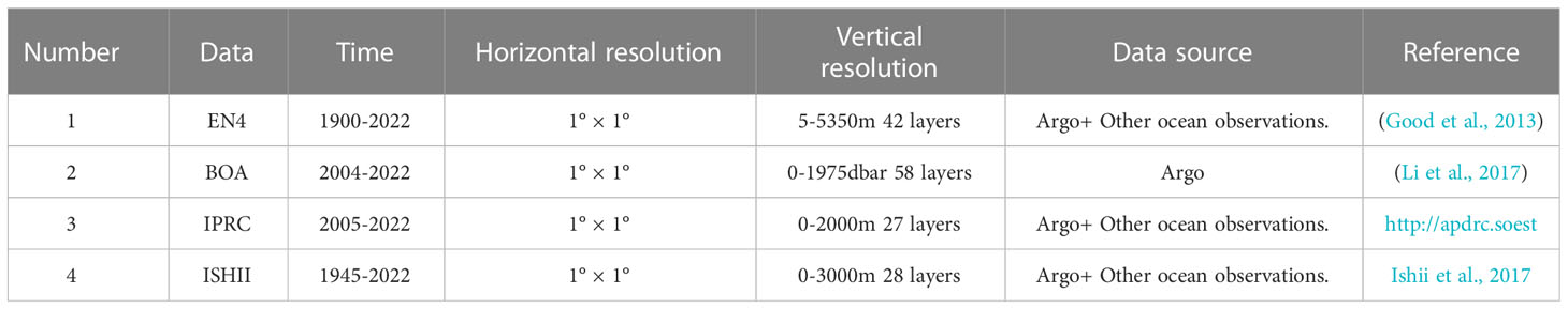
Table 1 Argo global temperature and salinity data.
2.2 Wind data
The wind stress field was computed with the help of the wind components (U and V components) and the 10 m wind speed information from ERA-Interim, which was developed by the European Center for Medium-Range Weather Forecasting (ECMWF). Since 1979, users have had access to this data on a monthly schedule, with a resolution of 1°×1° throughout the whole planet. Please refer to Dee et al. for more details about the ERA-Interim forecasting model, data assimilation methodologies, and input dataset (2011).
2.3 Climate data
This study used NCEP-NCAR monthly mean reanalysis of precipitation, evaporation, and heat flow data. This reanalysis dataset includes turbulent fluxes like sensible and latent heat fluxes and net radiation fluxes like net longwave and net shortwave radiation. Its resolution is 1.904°×1.825°. GECCO2 monthly mean reanalysis product temperature and salinity datasets were used to calculate advection. GECCO2, the German contribution to Estimating the Circulation and Climate of the Ocean, version-2, has a 1°×1° resolution (Köhl, 2014).
The ENSO event is characterized by the Niño3.4 index, which is defined as the spatial average of the sea surface temperature level field in the Niño3.4 region (150°E-170°W, 5°S-5°N). Positive (exceeding +0.5°C) and negative (lower than −0.5°C) values of the Niño 3.4 SST index, respectively, indicate El Niño and La Niña conditions. In this paper, the month-by-month average data is selected as the time series of Niño3.4 index. The data were mainly obtained from the website of Physical Sciences Laboratory (https://www.esrl.noaa.gov/psd/gcos_wgsp/Timeseries/Niño34).
This paper uses the National Oceanic and Atmospheric Administration (NOAA) NCEI PDO index data reconstructed on the basis of the fifth-generation version of the ERSST extension (https://www.ncdc.noaa.gov/teleconnections/pdo/). Generally, the PDO shifts phases on at least interdecadal time scale, usually about 20 to 30 years.
3 Methods
3.1 STL decomposition
The Seasonal-Trend decomposition based on Loess (STL) method, originally proposed by Cleveland et al. (1990), is a robust filtering algorithm designed to decompose time series data into distinct components, namely trend, seasonal, and residual subseries. By utilizing a series of loss (locally weighted scatterplot smoothing) operations, STL effectively disentangles long time series data, enabling the separation of linear trend patterns, interannual variability, periodic patterns, and residual fluctuations, as denoted by Equation (1). Yt is the observed value at time t, and Lt, It, Rt, and St represent the linear trend, interannual variation, periodic variation, and residual term at time t, respectively.
The computation process of the STL algorithm incorporates two iterative mechanisms: the inner loop and the outer loop. The inner loop is primarily dedicated to conducting component calculations for trend and seasonal components in time series data, resulting in improved trend fitting effects. Meanwhile, the outer loop is utilized to effectively mitigate the impact of outliers during each iteration of the component calculations. This enables the algorithm to derive robust computation weights that are less susceptible to the influence of extreme data points.
3.2 Steric sea level calculation
Calculation of SSLA, TSLA, and HSLA using ocean temperature and salinity was carried out as follows (Jayne et al., 2003; Llovel et al., 2013)
denotes the average density of seawater (1028 kg/m3), T、S; and p, respectively, stand for temperature, salinity, and pressure, while and are the mean temperature, mean salinity, and mean density, respectively. α and β are the thermal expansion and saline contraction coefficient, respectively, calculated from monthly temperature and salinity using the Thermodynamic Equation Of Seawater 2010 (TEOS-10). By taking the total differential, SSLA can be decomposed into TSLA and HSLA, which are mathematically expressed by Equations (3) and (4), respectively. SSLA, TSLA, and HSLA anomalies are estimated not only over 0–2000m but also for a specific layer between depths ‘z1’ and ‘z2’.
3.3 WSC calculation
Calculation of meridional and zonal surface wind stress and using the standard volumetric formula:
ρa=1.2 kg/m3 represents the reference air density, and represent the meridional and zonal components of the 10-meter wind vector, and represents the segmented drag coefficient used in the calculation (Large and Pond 1981).
The wind stress curl (WSC) is calculated as
A positive value for the WSC in the southern hemisphere is associated with a negative Ekman pumping velocity, which is the primary force behind upper-ocean convergence and the depression of isopycnal surfaces.
3.4 Temperature and salinity decomposition
Spicing and Heaving forms of subsurface temperature and salinity fluctuations in the ocean at various depths (Bindoff and McDougall, 1994; Häkkinen et al., 2016; Huang, 2020) give more insight into the causes of temperature and salinity changes. The Heaving mode is defined by temperature or salinity changes caused by thermocline undulations caused by adiabatic processes such as significant wind forcing or global warming. The Spicing mode depicts compensatory temperature and salinity fluctuations over the isopycnal surface, which are predominantly caused by changes in air-sea fluxes in water mass production zones or mixing processes along water mass routes. The separation of the Heaving and Spicing modes is possible because of the use of both depth and density dimensions. Potential temperature and salinity variations, observed at a depth expressed as (, can be decomposed using the following equation:
The variables θ and S represent potential temperature and salinity, respectively. The subscripts ρ and p denote measurements along the neutral density surfaces and at constant pressure, respectively. Assuming a constant vertical temperature gradient () over time, the first term on the right-hand side of equation (9) and equation (10) describes the temperature and salinity changes caused by Spicing, which is a consequence of mode changes. The second term on the right-hand side of equation (9) and equation (10) represents the temperature and salinity changes due to the Heaving of the thermocline. The annual variations of potential temperature (pressure) at constant density are denoted by (()while the long-term (2005-2019) mean values of temperature and potential density are denoted by . The salinity is calculated using a similar approach (Nagura and Kouketsu, 2018).
3.5 Ocean heat budget
To gain a deeper understanding of temperature change processes, a heat budget analysis was conducted for the 0-700 m layer of the Pacific Ocean:
represents the analytical heat transfer calculation for the advection term across four horizontal boundaries, T represents temperature, uH represents horizontal (meridional and zonal) circulation, and represents the horizontal gradient operator. The surface heat flux forcing term is denoted by Qv, where Qnet represents the total heat flux between the ocean and the atmosphere including sensible heat flux (Qshf), latent heat flux (), shortwave radiation (Qsw), and longwave radiation (Qlw). The reference density and heat capacity of seawater are represented by and , respectively. The residual term, Res, allows for the consideration of unresolved processes such as vertical and horizontal diffusion as well as errors in calculation. A detailed research flowchart of this study is presented in Figure 1.
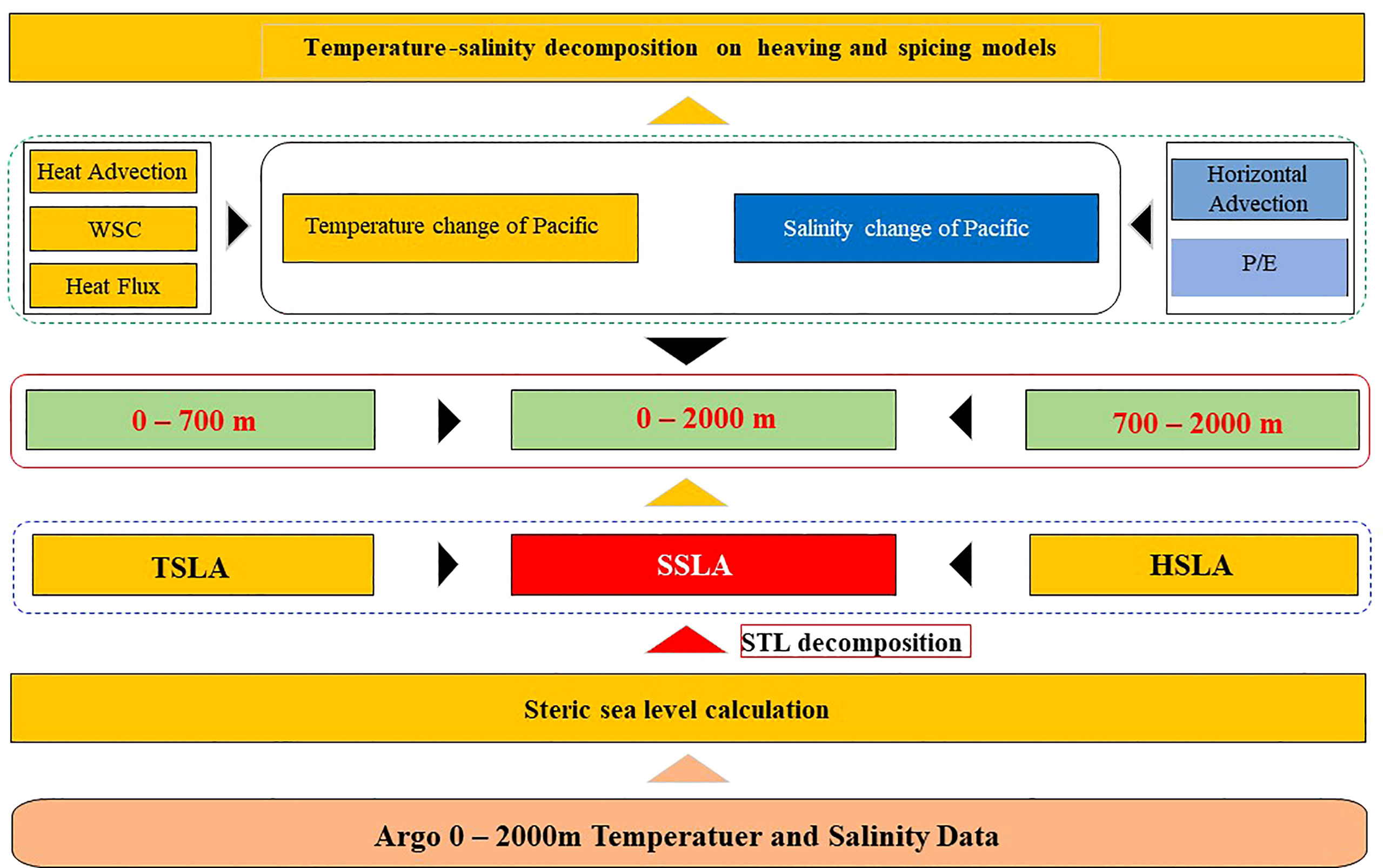
Figure 1 Flowchart for quantifying the contribution of temperature, salinity, and climate change to sea level rise in the Pacific Ocean.
4 Results and discussion
4.1 Global and Pacific interannual-to-decadal sea level change
This study utilizes data from IPRC, ISHII, EN4, and BOA to derive spatial distribution maps illustrating the spatiotemporal trends of global SSLA, TSLA, and HSLA during the period 2005-2019 (Figure 2). Remarkably, our findings are consistent with the SSLA results computed by the Copernicus Data Centre, further validating their accuracy and reliability. Figure 2 shows that despite an overall increase in sea levels across most regions globally, there are substantial geographical variations between the various oceanic areas. Sea levels in the North Indian Ocean, the Eastern Pacific Ocean, and the Atlantic Warm Pool display pronounced surges, significantly exceeding the global average sea level rise rate.
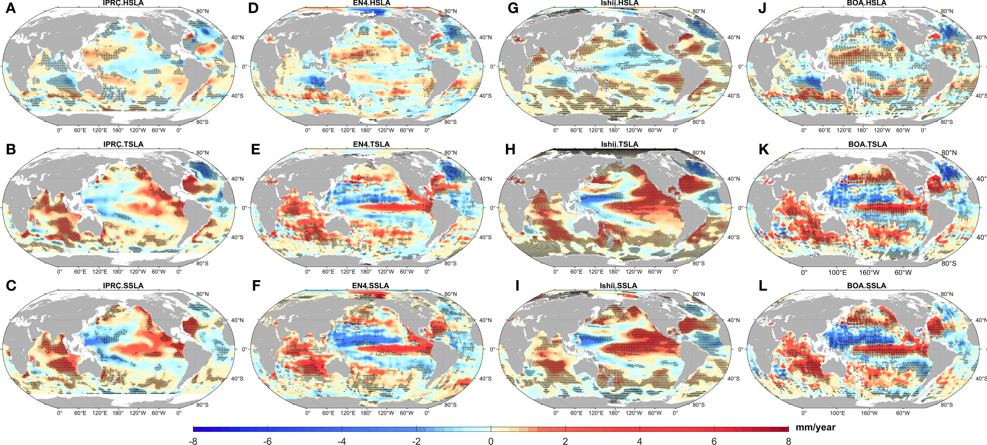
Figure 2 Linear trend maps of (A) halosteric sea-level anomaly (HSLA), (B) thermosteric sea-level anomaly (TSLA), and (C) steric sea-level anomaly (SSLA) for the 2005-2019 period derived from IPRC (D–L) are the same as (A–C) but derived from Ishii, BOA and EN4, respectively. Stippling indicates significance at 90% confidence level based on a Mann-Kendall test.
The Pacific steric sea level anomaly shows an overall positive trend, characterized by an amplified trend of SSLA in the South Pacific and Eastern Pacific and a markedly diminishing trend of SSLA in the Western and Subtropical Pacific. These patterns can be ascribed to El Niño events and oceanic heat transport, which have induced pronounced warming of the South Pacific and Eastern Pacific and propelled the upward trend of TSLA. Simultaneously reduced warming in the western Pacific has caused a decline in SSLA in this region.
A comparison of the first and second rows of Figure 2 demonstrates that the variability trend of TSLA generally outpaces that of HSLA and has a substantial role in influencing the changing trend of SSLA. This is revealed by the fact that TSLA’s trend of variability surpasses that of HSLA. HSLA variability also has a certain influence on the variability trend of SSLA, with all four datasets displaying significant positive HSLA trends in the Subtropical North Atlantic and subtropical Pacific, which contributes to the rise in SSLA. This influences the variability trend of SSLA in a certain way. The HSLA, on the other hand, is exhibiting major downward trends in the South Indian Ocean, the tropical and Subpolar North Atlantic and Tropical Pacific, which is reducing the growth in SSLA. It is essential to keep in mind that shifts in the salinity of the ocean are a primary factor in the variability of the sea level in these locations.
In the latitudinal range of 30°S to 50°S and 40°N to 60°N, there has been a clear increase in the upward trend of SSLA (Figure 2). Previous research (Germineaud et al., 2023; Qu and Melnichenko, 2023) suggests that the convergence of heat in the upper ocean and the downward Ekman suction induced by local wind forcing in high-latitude regions of the Pacific are related factors. This surface ocean warming leads to an increase in sea level due to thermal expansion. In the 10° ~ 40°N belt area of the western Pacific region there is a strong upward trend in HSLA but also a significant downward trend in SSLA due to a dominant downward trend in TSLA in this area. The calculated results from the four datasets all indicate a general upward trend in the Pacific Ocean’s Sea level. Based on this comparison, the focus of this study will be on the strong upward trend of SSLA and its relationship with ocean salinity and temperature from 2005 to 2019. We speculate that the rising sea levels in the high-latitude regions of the South Pacific may be attributed to the interaction between ENSO and the AAO wind forcings. Further investigation into the relationship between ENSO and the South Pacific AAO is warranted. However, such necessary efforts are beyond the scope of this study, and it is left for future research.
The time series of steric sea level anomalies were processed using the STL method to remove seasonal variability and extract interannual variations. A 3-month sliding filter was then applied to obtain the interannual time series of SSLA, TSLA, and HSLA (Figure 3). The SSLA displayed significant interdecadal variations in its rising trend over the past half-century, with a more pronounced increase becoming apparent after 1990 (although the signal before 1990 was weak). Furthermore, based on IPRC estimation, the SSLA trend between 2005 and 2019 was 0.34 ± 0.16 mm/yr (with a ±90% confidence interval based on the F-test). The results from Ishii, EN4, and BOA were consistent with IPRC, indicating an accelerating rising trend of SSLA in the Pacific Ocean since 2005. A comparison of TSLA and SSLA found that the decadal variability in SSLA is primarily derived from TSLA. Previous research showed that interannual sea level variations in the tropical Pacific are largely influenced by ENSO dynamics and associated heat redistribution (Palmer et al., 2019). Our findings further confirm that SSLA interannual variations in the Pacific region during 2005-2019 are predominantly driven by El Niño events in the Pacific area and PDO in the North Pacific.
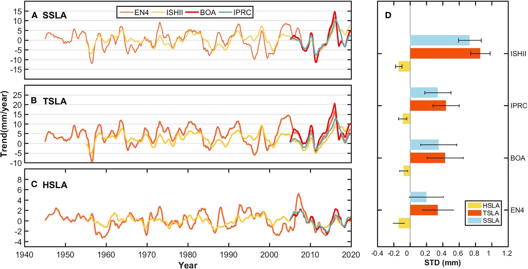
Figure 3 Annual (A) SSLA, (B) TSLA, (C) HSLA in the Pacific Ocean based on the EN4, Ishii, BOA, and IPRC datasets, and (D) Linear trends and standard deviations of SSLA (blue bars), TSLA (red bars), and HSLA (yellow bars) in the Pacific Ocean during 2005-2019 based on BOA, EN4, IPRC, and Ishii datasets. Error bars represent 90% confidence intervals based on the F-test.
As shown in Figure 4A, Pacific TSLA and SSLA interannual variations are well-correlated with the 1.5-year low-pass-filtered Niño 3.4 index (correlation estimation of 0.8, significant at the 95% level, with zero time lag) and the PDO index (correlation estimation of 0.75, significant at the 95% level, with a one-month time lag). Figure 4B demonstrates that the interannual variations in the 0-700m layer of the Pacific from 2005-2019 are more pronounced in the region north of the equator, dominating SSLA changes across the entire Pacific. To further analyze the cause of Pacific interannual variations, we quantified the SSLA trends in the North and South Pacific regions separately (Figure 5). The calculations based on the Ishii temperature and salinity data reveal that the SSLA trend in the North Pacific (0°-60°N) is 0.56 mm/yr, whereas the SSLA trend in the South Pacific (0°-60°S) is 0.20 mm/yr. The rate of SSLA rise in the North Pacific was nearly twice the rate of rise in the South Pacific, and the results of this paper were in general agreement with those calculated by Zuo et al. (2009). Comparing Figures 5A and B , we observe that the SSLA amplitude in the North Pacific is markedly larger than that in the South Pacific. Additionally, the sum of the trends in both regions (Figure 5C) almost aligns with the overall trend of SSLA in the Pacific, indirectly validating the feasibility of our regional averaging methodology.
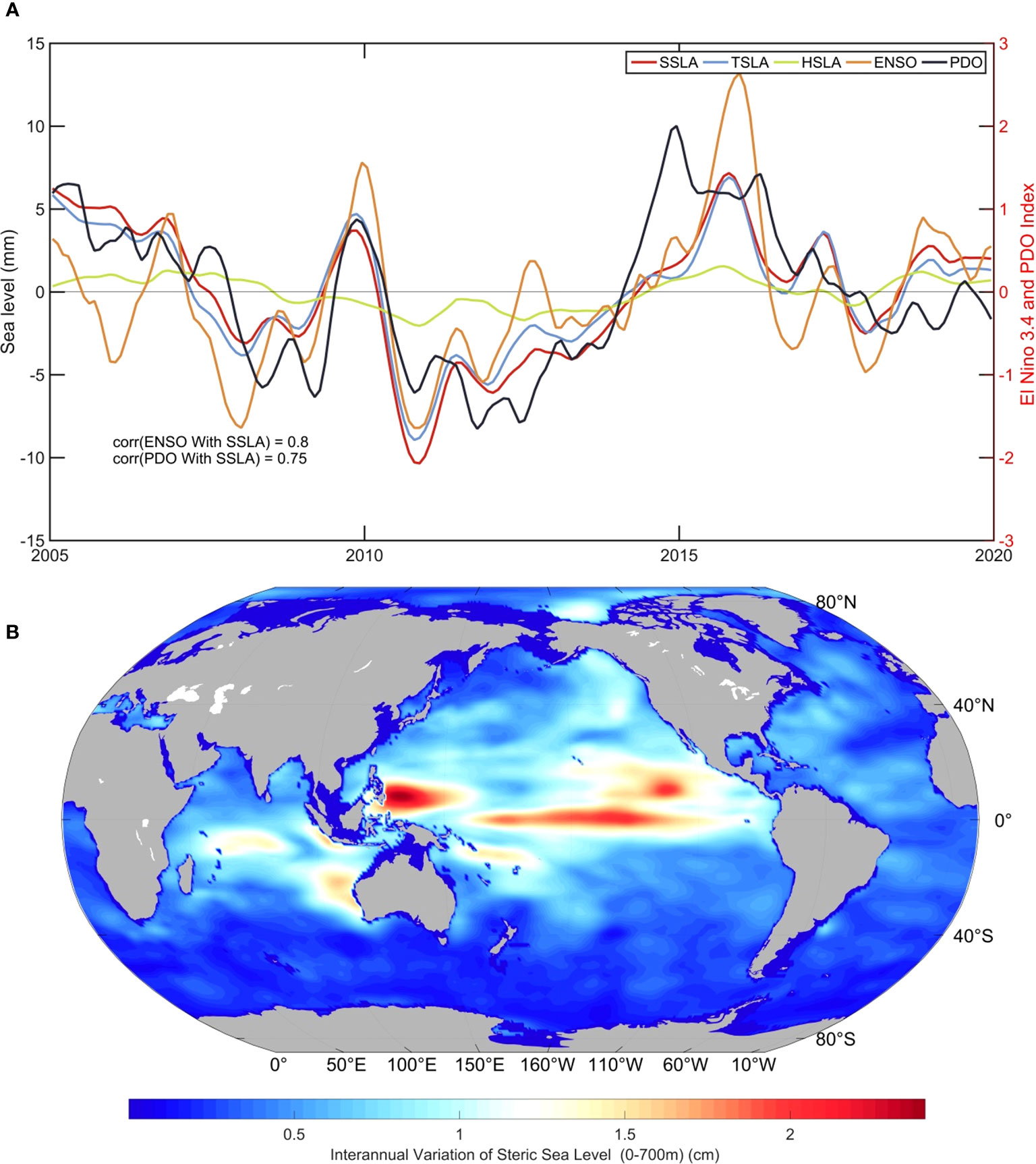
Figure 4 (A) Interannual variation of SSLA (red), TSLA (blue), HSLA (green) based on Ishii data, and 1.5x low-pass filtered PDO (pink) index, El Nino 3.4(orange) index of the Pacific Ocean calculated for correlation comparison; (B) Spatial distribution of interannual variation of SSLA in 0-700m layer calculated by Ishii data from 2005-2019.
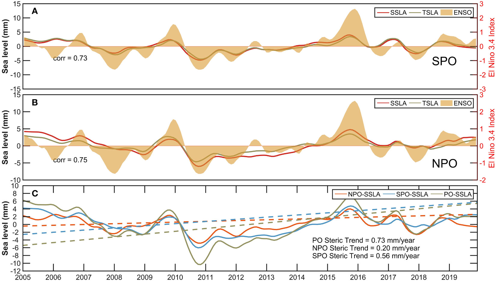
Figure 5 Interannual variation of (A) SSLA, TSLA, El Nino 3.4 index for the South Pacific Ocean (SPO), (B) as for (A), but for the North Pacific Ocean (NPO), (C) SSLA, interannual variation of SPO (blue), NPO (orange) and PO (green), and trends based on Ishii, 2005-2019.
Existing studies (Palanisamy et al., 2015) have shown that the North Pacific is mainly modulated by the PDO. The findings above indicated that, during this period, the specific volume sea level changes in the Pacific are notably regulated by ENSO and PDO. Yet, it is noteworthy that SSLA exhibits a slightly diminished long-term ascending trend when compared to TSLA. This disparity can be attributed to the presence of a negative trend displayed by HSLA during extended temporal variations, which exerts a negative influence on the overall trend of SSLA. The trend in TSLA from IPRC is 0.44 ± 0.16 mm/year, accounting for approximately 84% of the SSLA trend (as shown in Figure 3D). The HSLA shows a persistent decline from 2005 to 2015, with insignificant interannual and decadal fluctuations,with a trend of -0.09 ± 0.05 mm/year accounting for approximately 16% of the SSLA trend and exhibiting a downward trend in all four datasets.
4.2 Contribution of temperature and salinity at different depths to sea level rise
This paper investigates how variations in salinity and temperature across different ocean depths (0-700m, 700-1000m, 700-2000m, and 0-2000m) revealed by the BOA, EN4, IPRC, and ISHII datasets impact the trends of TSLA and HSLA. Figure 6 illustrates spatiotemporal changes in temperature and salinity from 2005 to 2019. All four datasets indicate a marked warming trend in the Pacific Ocean at depths greater than 1000m since 2015 (Figure 6). This warming trend is most evident in the 0-700m layer, which had previously shown a cooling trend from 2005 to 2014. The 700-1000m layer displays interannual variability in temperature, with warming anomalies observed during 2008-2010 and 2012-2014, and cooling anomalies during 2016-2018 despite overall warming across all layers during that period. Although the 0-700m ocean layer exhibited a cooling trend from 2006 to 2015, a rapid warming phenomenon emerged in the upper ocean layer since 2015, lasting until 2016, followed by a weakening trend. Existing research suggests that this phenomenon was triggered by the strong El Niño event in 2015-2016, which marked the first extreme climate variation of the 21st century (McPhaden, 2015). During this event, the easterly trade winds in the tropical Pacific weakened, and westerly winds intensified, leading to changes in the direction and velocity of equatorial currents. Consequently, the warm pool shifted eastward, causing sea surface temperature anomalies in the tropical Pacific region (McPhaden, 2015; Wu et al., 2018; Wu and He, 2019; Zhi et al., 2019; Yu et al., 2021; Zou and Xi, 2021; Tang et al., 2022; Germineaud et al., 2023; Hu et al., 2023). At the peak of the 2015 El Niño event, tropical eastern Pacific temperatures increased by 3°C (Kusuma and Nur, 2020), resulting in extensive heat redistribution and associated sea level changes in the tropical Pacific and mid-latitude South Pacific regions (Germineaud et al., 2023), which led to an increasing trend in TSLA. The shift from cooling to rapid warming was a key driver of the rise in TSLA after 2015. Salinity variations are more pronounced than temperature variations in the 0-700m and 700-1000m layers. The 0-700m layer exhibits a negative correlation between salinity and temperature and displays significant interannual variability. In contrast, the 700-1000m layer shows a sustained long-term trend of haline contraction, and an increasing trend in salinity after 2015. This trend may represent the primary driver of the unchanged trend in HSLA at depths of 0-2000 m.
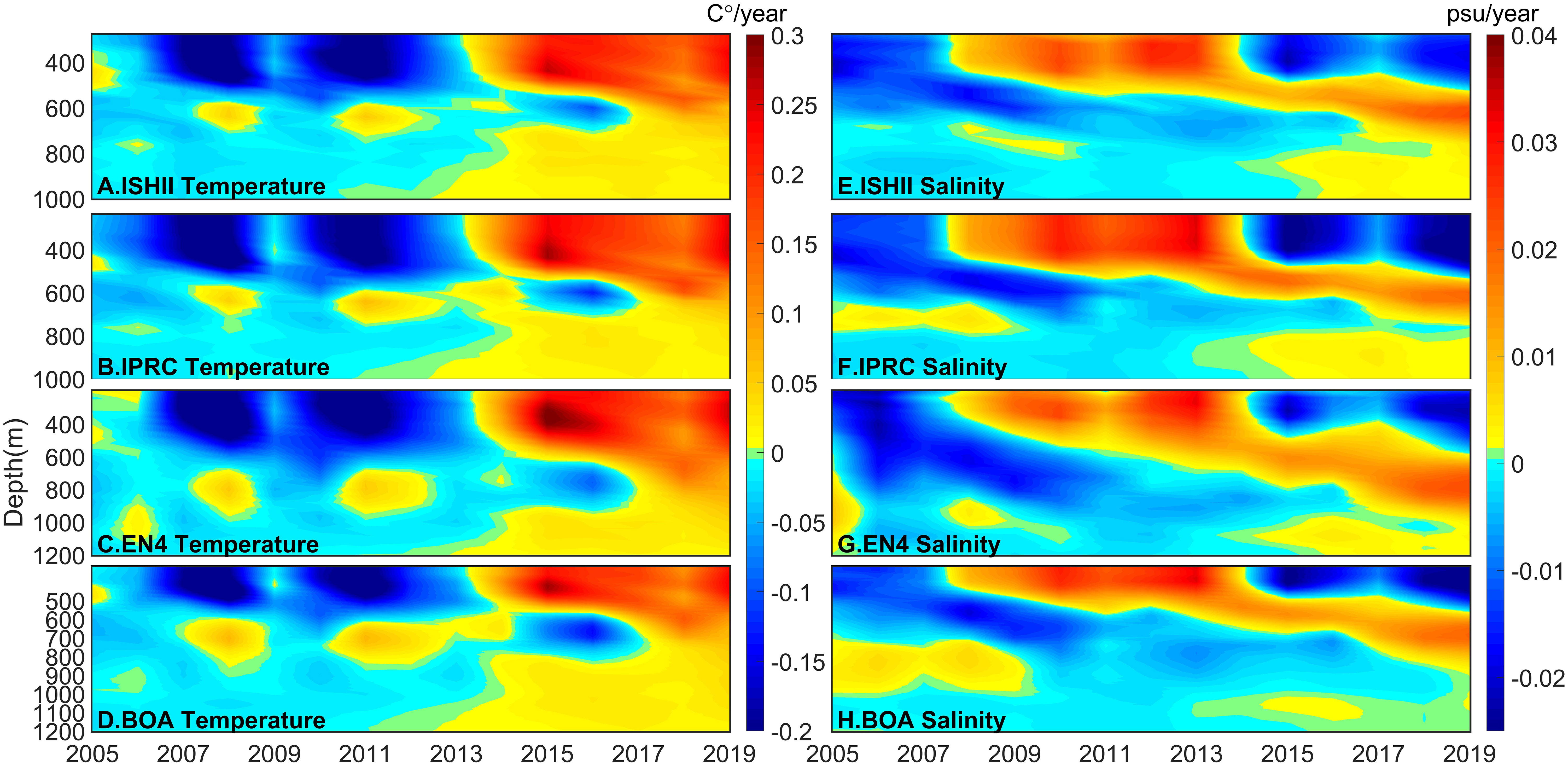
Figure 6 (A) Ishii, (B) IPRC, (C) EN4, and (D) BOA based temperature anomaly changes in the upper 1000 meters of the Pacific Ocean. (E–H) Salinity anomaly changes in the same region as temperature, based on the same datasets.
On the basis of these comparisons, in order to gain a deeper comprehension of the roles that temperature and salinity play at varying depths in determining SSLA variations, separate calculations were conducted for TSLA and HSLA at depths of 0-700m and 700-2000m, using observational data from BOA, EN4, IPRC, and ISHII, and then compared with overall results for the 0-2000m layer. IPRC calculations indicated that, from 2005 to 2019, the SSLA trends for the 0-700m and 700-2000m layers were 0.33 ± 0.11 mm/yr and 0.01 ± 0.007 mm/yr (Figure 7), respectively accounting for 97% and 3% of the SSLA trend in the 0-2000m layer. Similar results were obtained from other datasets, all of which indicated that the 0-700m layer had a greater impact on sea level change than the 700-2000m layer. The trend of IPRC TSLA in the 0-700m layer was 0.44 ± 0.16 mm/yr (Figure 7), which determined the overall trend of TSLA, while the trend in the 700-2000m layer was weak and had a smaller impact on the overall trend of TSLA.
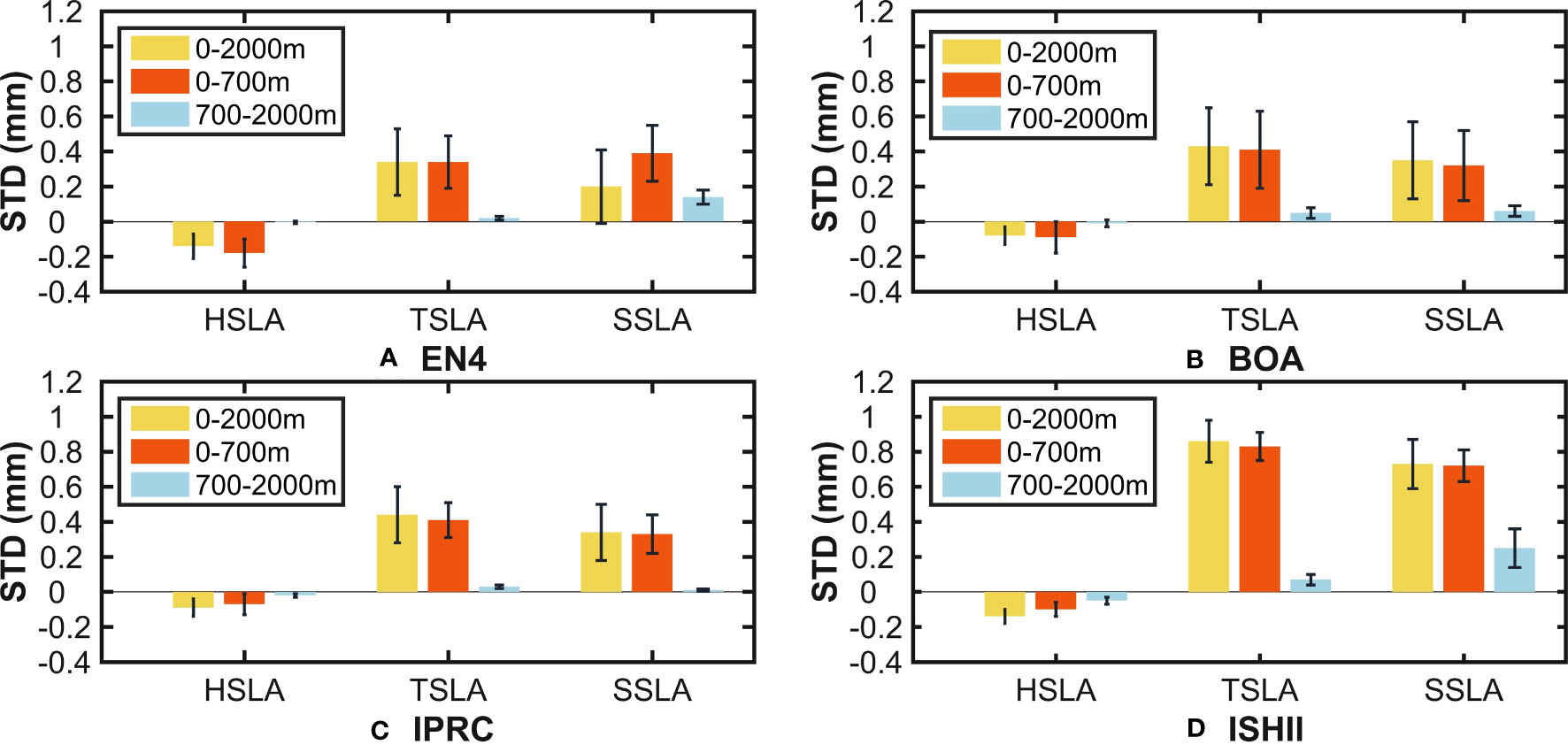
Figure 7 Linear trends of SSLA, TSLA, and HSLA were calculated for the 0-2000m (yellow bars), 0-700m (red bars), and 700-2000m (blue bars) layers during 2005-2019. The data are from (A) EN4, (B) BOA, (C) IPRC, and (D) Ishii. Error bars represent the 90% confidence intervals based on the F-test.
The trend of IPRC HSLA in the 0-700m layer was -0.07 ± 0.06 mm/yr, which accounted for approximately 78% of the HSLA trend in the 0-2000m layer and was primarily influenced by interannual variability in upper Pacific salinity. The trend of HSLA in the 700-2000m layer was 0.02 ± 0.01 mm/yr, representing approximately 22% of the HSLA trend in the 0-2000m layer, and exhibiting no significant long-term trend. The contribution of the 0-700m layer was significantly greater than that of the 700-2000m layer. Results from all four datasets indicated a negative and indeterminate trend in HSLA contributions to the Pacific.
Based on IPRC data, the trend in SSLA in the 0-700 meter layer of the Pacific Ocean during the period 2005-2019 is estimated to be 0.33 ± 0.11 mm/yr, and dominated the trend in SSLA for the 0-2000 meter layer. This contribution is primarily attributed to the warming of the upper ocean (TSLA), with a secondary role played by changes in salinity (which account for 17% of the contribution according to IPRC data). Specifically, the trend in SSLA for the 0-700 meter layer is estimated to be 0.33 ± 0.11 mm/yr, accounting for approximately 93% of the SSLA rise in the 0-2000 meter layer, while the SSLA trend for the 700-2000 meter layer is weaker, at 0.03 ± 0.01 mm/yr (Figure 7). The results obtained from BOA, Ishii, and EN4 are generally consistent with those from IPRC. A comprehensive analysis of these combined results suggests that sea level change in the Pacific Ocean is mainly influenced by the temperature and salinity of the upper 0-700 meter layer of seawater, and the observed causes affecting sea level change in the Pacific Ocean are characterized by significant complexity.
4.3 The reasons for temperature and salinity variations
4.3.1 Heaving and spicing anomalies
Utilizing the IPRC dataset, temperature and salinity changes within the Pacific Ocean’s 0-700 meter layer were decomposed and calculated using formulas 9 and 10, producing the Heaving and Spicing modes of the layer (Figure 8). The Heaving mode exhibits a warming trend in the upper ocean and considerable interannual variability in the 0-700 meter layer. The temperature changes observed within the Heaving mode predominantly reflect fluctuations of the thermocline layer, a phenomenon known to be influenced by Pacific trade winds (Figures 8A–C). El Niño events can induce atmospheric convergence near the equatorial International Date Line, causing anomalous east winds in the eastern Pacific and west winds in the western Pacific. This, in turn, deepens the thermocline layer, heightens stratification, weakens vertical convection, causes marked warming in the sub-surface layer, augments the ocean’s heat absorption capacity, and eventually culminates in sea level rise within the central equatorial Pacific. Conversely, the Spicing mode has minimal effects on temperature changes, indicating that the chief mechanism causing isopycnic temperature variations in the ocean’s interior is a fluctuation of the thermocline layer. The downward (or upward) movement of the thermocline layer prompts fixed-level warming (or cooling), concomitant with alterations in seawater density. Downward movement of the thermocline layer induces an elevation in sea surface temperature, which consequently drives the upward trajectory of TSLA.
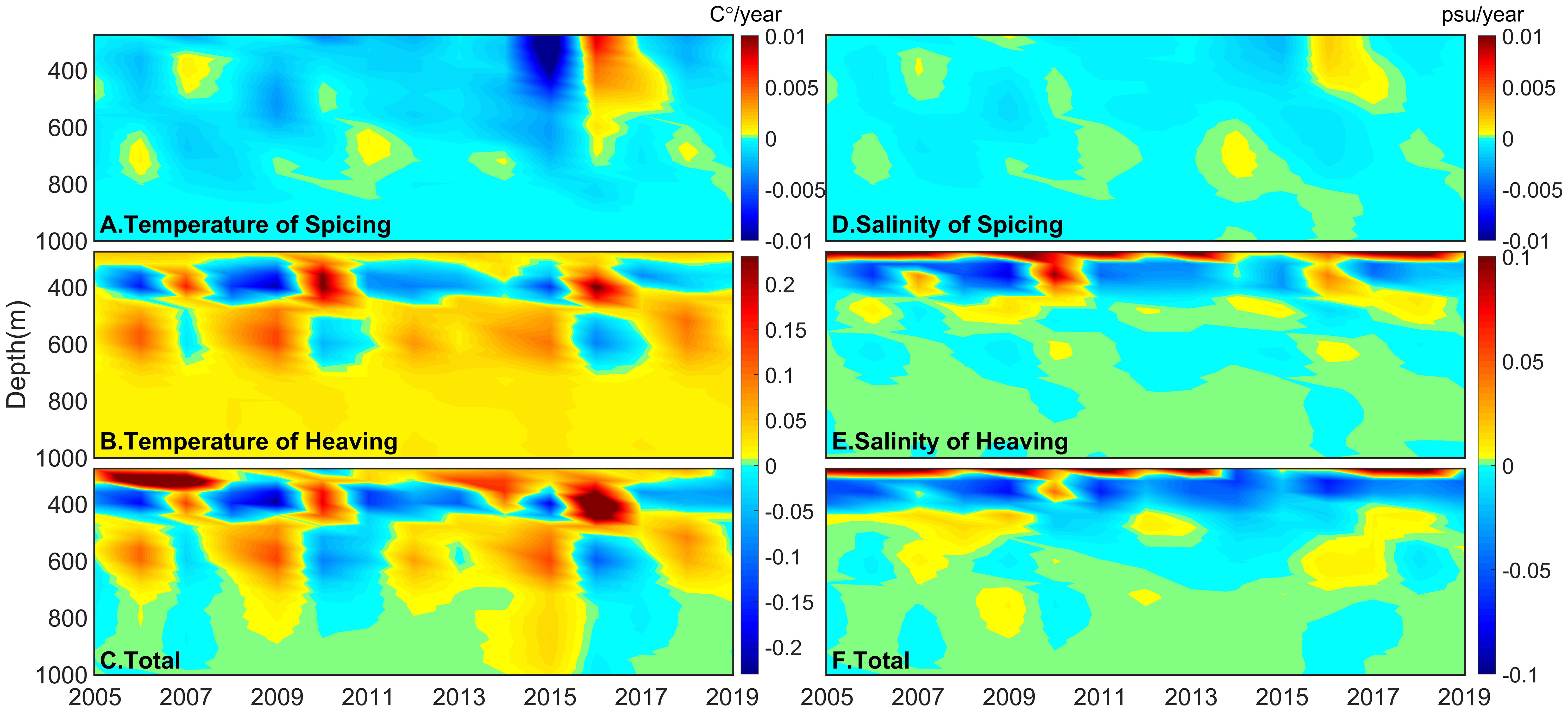
Figure 8 Temperature anomalies of (A) the Spicing mode, (B) the Heaving mode, and (C) their sum in the upper 1000 m averaged over the Pacific, derived from IPRC, (D–F) Same as (A–C) but for salinity anomalies.
Figures 8D–F illustrates the crucial role of the heaving mode in driving salinity changes, as this mode displays remarkable interannual variability. Notably, periods of thermocline descent occurring during 2010-2011 and 2015-2016 coincide with anomalous salinity increases. Conversely, throughout most other time intervals, a freshening trend is observed in the 0-700m layer within the heaving mode. Additionally, the Spicing mode is characterized by a freshening trend in the 700-1000m seawater layer, corresponding to a density range of 26.3-27.6 kg/m3. This layer constitutes the active region for the Sub-Antarctic Mode Water (SAMW) and the Antarctic Intermediate Water (AAIW). Overall, this study underscores the importance of the heaving and Spicing modes in governing salinity changes in the Southern Ocean, thereby elucidating the complex dynamics governing regional ocean circulation and climate patterns. (e.g., McCartney and Talley, 1982; Hanawa and D.Talley, 2001; Sallée et al., 2006; Koch-Larrouy et al., 2010; Schmidtko and Johnson, 2012; Hong et al., 2020; Zhang et al., 2021).
Figure 9 reveals that, within the density range of 26.3-27.6 kg/m3, both temperature and salinity exhibit simultaneous rising trends during 2010-2011 and 2015-2016. Conversely, declining trends are observed for the periods 2005-2010 and 2016-2019. These findings indicate that the Pacific experiences continuous influxes of the Sub-Antarctic Mode Water (SAMW) and Antarctic Intermediate Water (AAIW) water masses along the southern boundary. Previous studies (e.g., Wong et al., 1999; Bindoff and McDougall, 2000; Durack and Wijffels, 2010; Durack, 2015; Swart et al., 2018) have reported large-scale freshening trends in the Pacific’s SAMW and AAIW. This freshening, attributed to circulation gyres and eddy transport, results in localized seawater freshening in specific regions of the Pacific. However, the satisfying influence of El Niño events and the Pacific warm pool offsets this freshening trend, leading to increased seawater salinity and a decline in HSLA. These results highlight the pivotal role that ventilated water masses play in transmitting climate change signals to regional oceans, with significant consequences for regional sea level changes.
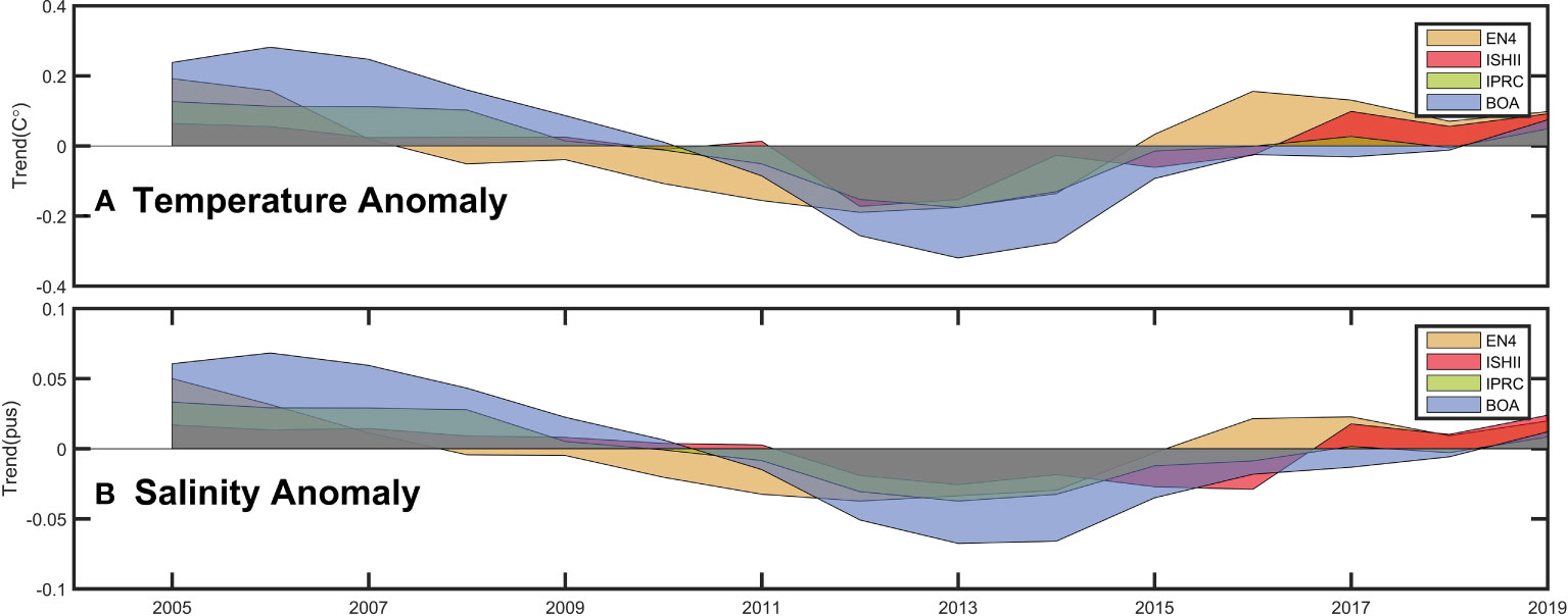
Figure 9 (A) Annual potential temperature anomalies averaged between 26.5-27.4 kg/m3 isopycnal surfaces in the PO derived from EN4 (yellow), Ishii (red), IPRC (green), and BOA (blue). (B) Same as (A) but for salinity anomalies.
4.3.2 Salinity analysis within the 0-700m layer
The global distribution of ocean salinity reflects the long-term balance between surface freshwater flux (E-P) and oceanic advection-mixing processes on a large scale. Therefore, any changes in the hydrological cycle are reflected in the ocean salinity field. To better understand the causes of ocean salinity changes, the freshwater budget of the Pacific Ocean from 0-700 m was examined using GECCO2 and ERA-interim reanalysis data (Figure 10). The findings reveal that the surface freshwater forcing (E-P) has a secondary influence on the observed salinity trend, with the advection term (Advs) being the primary contributing factor, as evidenced by a correlation coefficient 0.8. It is clear that Advs and E-P is mutually dependent on some salinity trends since both are closely linked to the tropical Pacific climate. Advection was also analyzed at a variety of boundaries, and the results suggested that salinity advection at the eastern, western, and northern limits is also an important component of the total Advs, which reveals complex circulation changes in the region. Interannual changes in E-P are mostly controlled by precipitation, but evaporation shows a slight trend towards rising over time. There has been a noticeable decrease in precipitation in the Pacific since 2014, and the enhanced evaporation that has been recorded in the region may be linked to the expansion of the global water cycle. This is despite the fact that precipitation in the Pacific continues to be considerable. The freshening tendency that is driven by ocean advection can be mitigated by increasing surface freshwater flow into the atmosphere, which also helps to offset the ascending trend of high salinity, and low oxygen water.
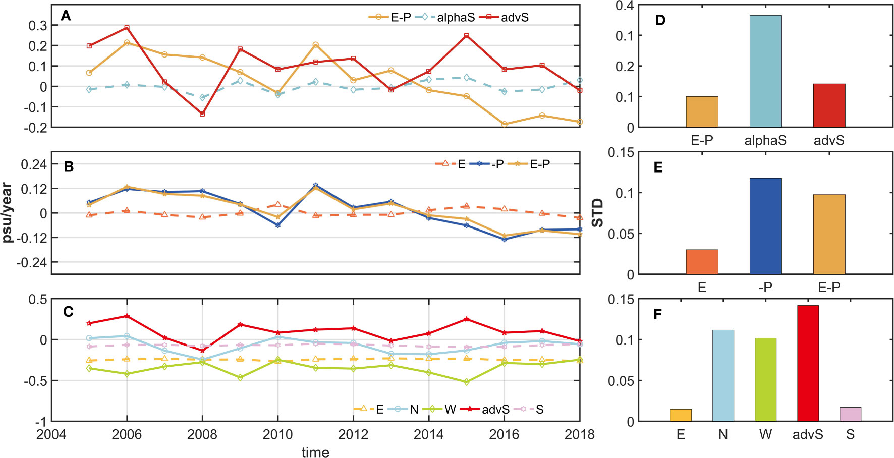
Figure 10 Salt budget in the upper layer (0-700 m) of the Pacific Ocean: (A) Salinity trend (blue, ∂S/∂T), surface freshwater flux (yellow, E-P), and horizontal advection term (red, Advs), from GECCO2 monthly-mean data, smoothed with a 12-month moving average. (B) Surface freshwater flux (E-P), with evaporation (Orange, E) and precipitation (blue, -P) shown separately. (C) Components of Advs, with E (yellow), W(green), N(blue), and S(pink) indicating the zonal, meridional, northern, and southern advection across the Pacific boundary (i.e., 700 m depth). (D–F) show the standard deviation of (A–C), respectively.
4.3.3 Warmth analysis from 0-700 meters
Temperature variations within the upper ocean are governed by both surface heat fluxes and oceanic dynamics. To better understand the underlying causes of warming in the Pacific region, a heat budget analysis and wind stress change analysis were carried out over the 0-700m depth range. GECCO2 model data were utilized to conduct the heat budget analysis, which provides a reasonably faithful representation of the temperature changes occurring in the Pacific Ocean at depths ranging from 0-700m, particularly the intensified warming pattern observed after 1990. However, the results of the calculations, which are presented in Figure 11, imply that there may be unresolved processes in the heat budget. These processes, which may include vertical and horizontal diffusion, are not capable of being resolved satisfactorily by the model. Because of these methodological limitations, an accurate estimate of the heat budget is difficult, leading to significant uncertainty in both Advt and HFF estimates.
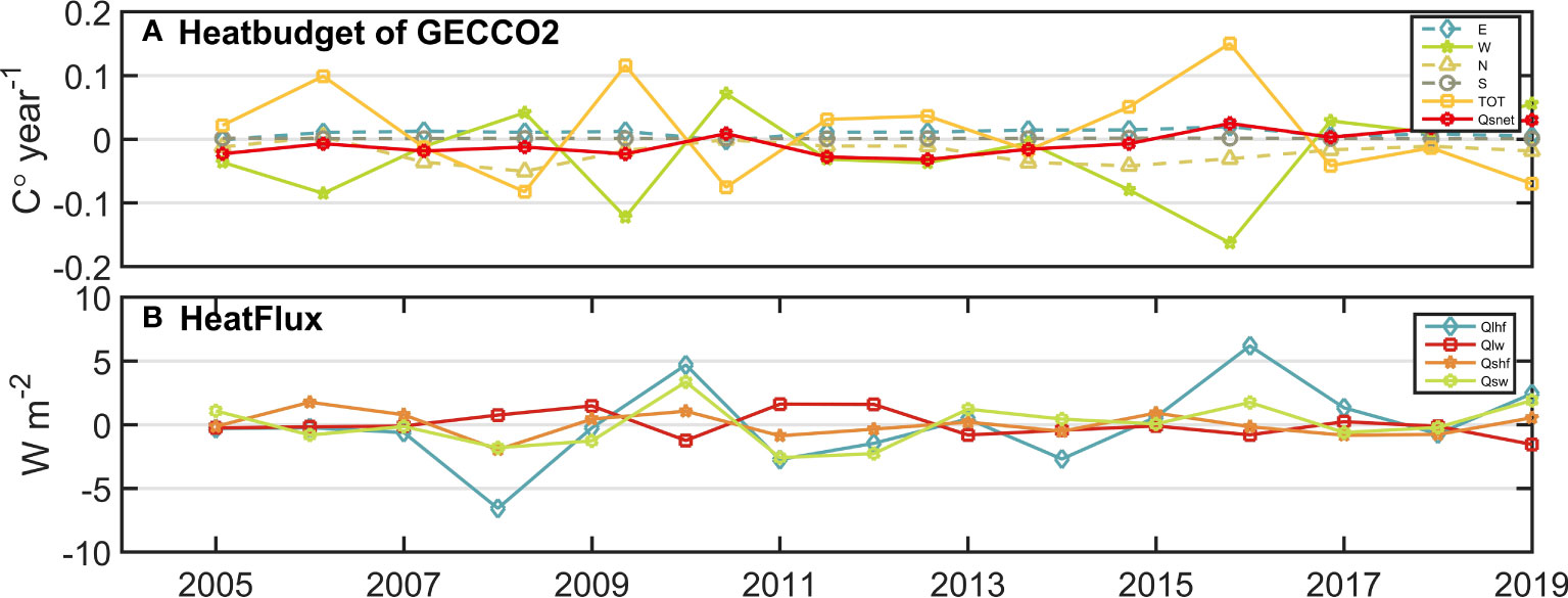
Figure 11 Upper ocean temperature budget in the Pacific: (A) heat advection at the eastern boundary (blue, W), western boundary (green, W), northern boundary (pale yellow, N), southern boundary (brown, N), total horizontal advection (deep yellow, TOT), and net heat flux (red, Qsnet) from monthly mean GECCO2 data, smoothed using a 12-month running average. (B) Qlhf (blue), QShf (yellow), QSW (green), and Qlw (red) represent latent heat flux, sensible heat flux, shortwave radiation, and longwave radiation, respectively.
GECCO2 allows for the correction of surface heat fluxes to achieve a better match between simulated and observed temperatures. When calculating Advt using monthly averaged data, large estimation errors may arise due to the nonlinearity of the advection term. Nonlinearity may be particularly strong in the Pacific region, which is characterized by enhanced eddy activity (Jia et al., 2011; Guo et al., 2020). We decomposed horizontal advection into four sub-components that represent heat advection in the northern, southern, eastern, and western Pacific regions, with their variations being determined by advection fluxes at the respective boundaries. Figure 11 presents the temporal variability of horizontal advection from 2005 to 2019, demonstrating significant periodicity and interannual variability, primarily influenced by advection from the western and eastern boundaries. During 2015-2016, a notable amplification of heat transport within the Pacific was observed, characterized by a reduction in westward heat flow and an increase in eastward-flowing currents in the tropical Pacific region (Figure 12). The enhanced eastward currents propelled the eastward migration of the warm pool, consequently inducing a substantial influx of heat into the eastern and southern Pacific domains. This phenomenon led to anomalous sea surface temperatures in the tropical Pacific and a rapid escalation of sea level temperatures, thereby driving the observed TSLA increase. Extant research has postulated a linkage between these occurrences and the strong El Niño event of 2015-2016 (Zou and Xi, 2021), further elucidating the underlying mechanisms responsible for these observed alterations
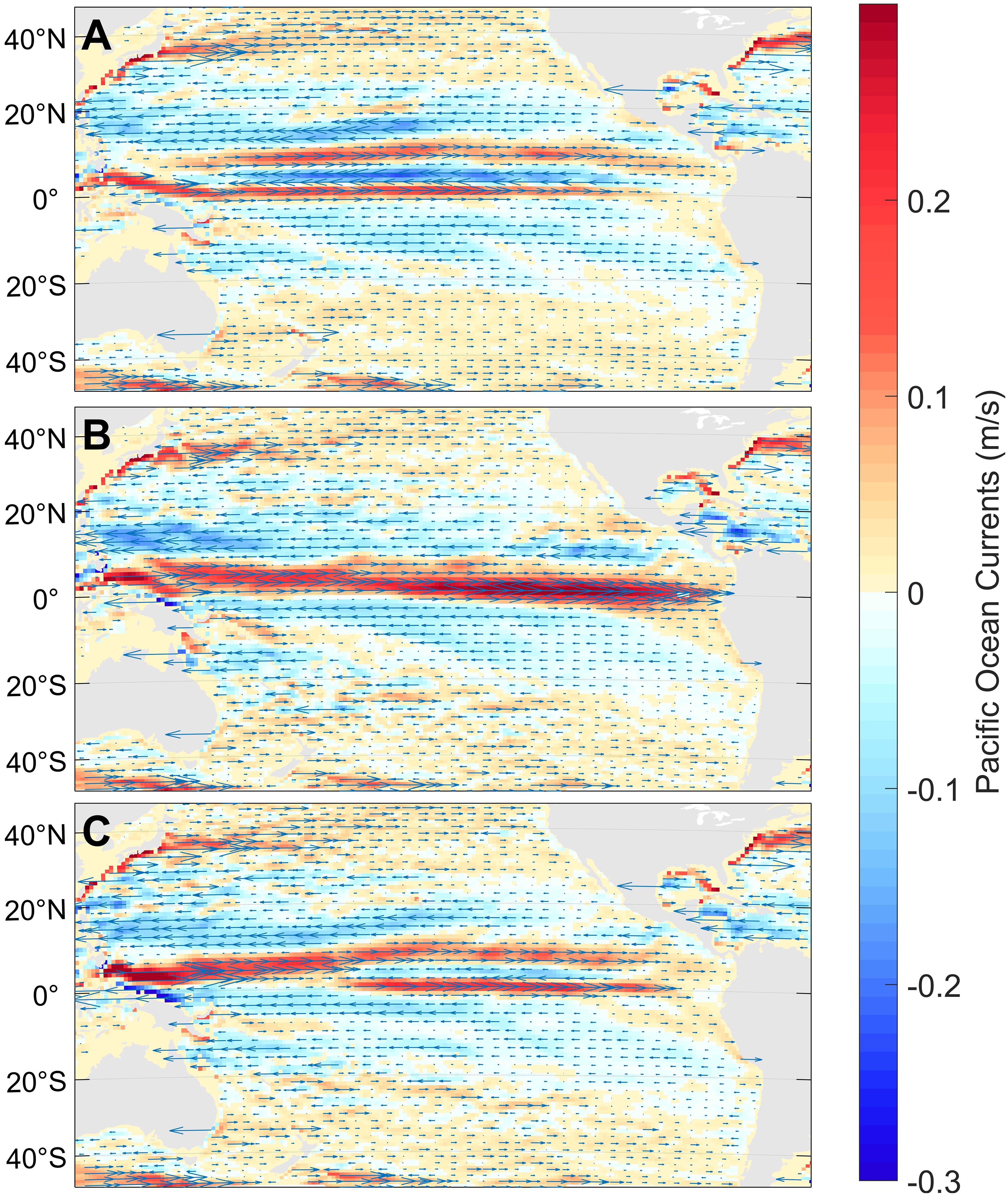
Figure 12 Pacific Ocean (A) 2016 (B) 2015, (C) 2014 Current distribution, shaded part is the current velocity, arrow is the direction of the current.
Figure 11 depicts the temporal evolution of surface heat flux parameters in the Pacific region. The latent heat flux (LHF) has assumed a dominant role in driving surface heat flux variability across the Pacific Ocean. Notably, there has been an observed upward trend in the latent heat flux (Qlhf), resulting in intensified evaporation of seawater. Consequently, this increased evaporation leads to the transformation of seawater into vapor, which subsequently accumulates as a greenhouse gas in the atmosphere above the sea surface. The augmented greenhouse effect arising from these processes has contributed to the warming of the sea level. Figure 11 also illustrates that both net surface heat flux and horizontal advection contributed to the warming of the upper Pacific Ocean, reflected in the increasing trend of TSLA. However, the sum of Advt and HFF does not explain the warming in the Pacific Ocean. Our findings shed light on the intricacy of the temporal variability of ocean thermodynamics in the Pacific, which poses a significant challenge for model simulations. Nevertheless, the results in Figure 11 offer a consensus on two potential processes that may have propelled the acceleration in warming since 1990, namely the amplification of warm currents triggered by El Niño events, and the augmentation of surface longwave radiation.
In the field of climate science, it is recognized that the Pacific Warm Pool is primarily affected by the trade winds in the tropical and subtropical regions that are subject to positive wind stress curl (WSC) in the subtropical zone (Figure 13), which facilitates the convergence of upper ocean heat. The western side of the majority of the Pacific area demonstrates an increasing trend in WSC. Surface wind shifts amplify the local Ekman downwelling and thermocline sinking that is associated with an upwelling pattern. The subsidence in the Pacific Ocean can be attributed to a concentration of heat in the top ocean.
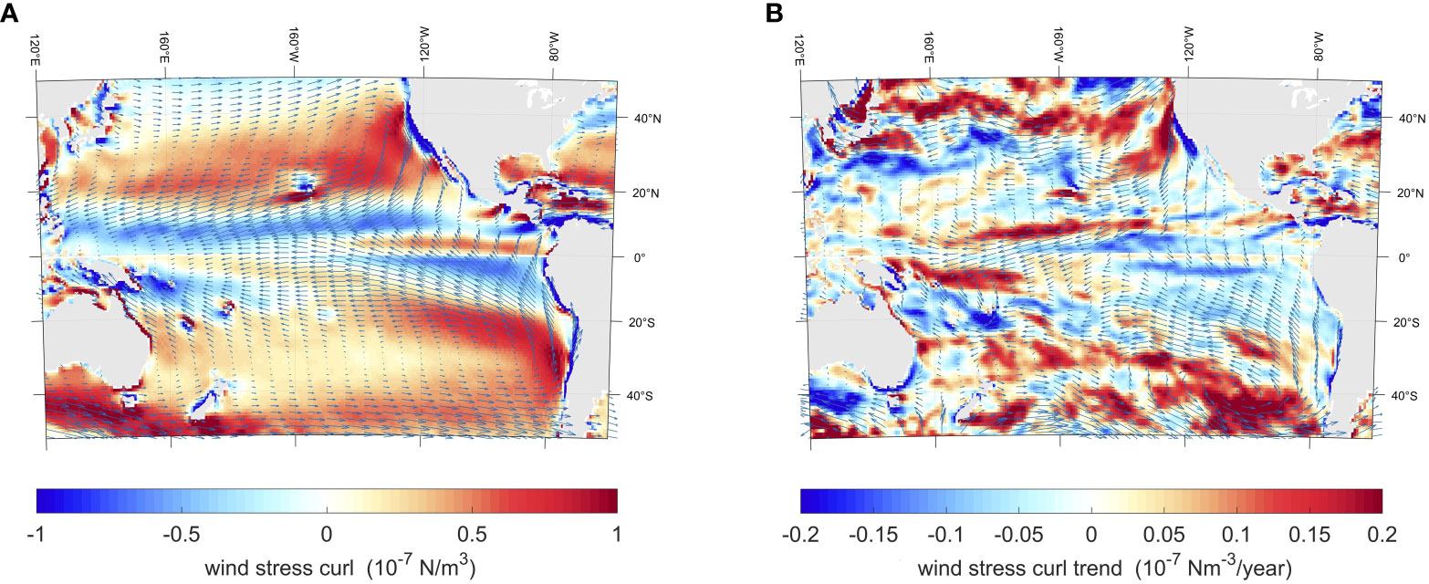
Figure 13 (A) Annual mean climatological surface wind stress (vectors; N/m2) and wind stress curl (color shading: 10-7 N/m3), (B) Linear trends of surface wind stress (vectors: N/m2) and wind stress curl shown in shading from ERA-20C for the period of 2005-2019.
In the realm of climate science, variations in the trade winds along the Pacific Ocean have become a critical factor in comprehending the mechanisms behind surface ocean warming and cooling. The enhanced greenhouse effect intensifies the processes of energy absorption and re-radiation at the surface of the oceans, leading to an increase in sea surface temperature. Simultaneously, it reduces the energy escape of net longwave radiation from the ocean surface (Frölicher et al., 2015; Lu et al., 2022). Figure 14 illustrates the spatial distribution of Qlw from 2005 to 2019, revealing quasi-uniform growth in the world’s oceans, which aligns with the fundamental features of anthropogenic greenhouse gas forcing. These outcomes also suggest that the composite influence of anthropogenic radiative forcing and wind-driven heat convergence has expedited the warming of the upper ocean and the rise of TSLA since 2005.
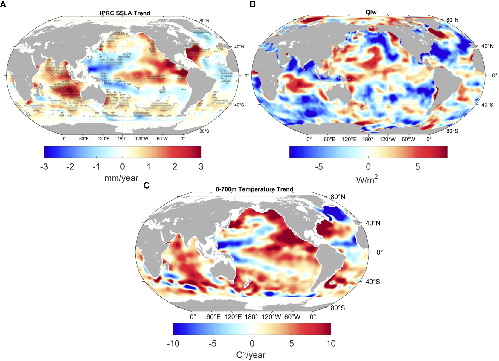
Figure 14 (A) The trend of 0-700 m SSLA computed by IPRC from 2005 to 2019; (B) the Trend of net Qlw at the sea surface variation from 2005 to 2019 based on NEPC-NACR data; (C) the Trend of temperature variation from 2005 to 2019 computed by IPRC for 0-700 m depth.
5 Conclusion
This study examines the spatiotemporal dynamics of the Pacific steric sea level anomaly and its driving mechanisms in light of its intricate circulation characteristics and the persistent influence of climate change. By harnessing ocean temperature and salinity measurements from four distinct Argo data sources, alongside climate data spanning the years 2005 to 2019, we conducted an in-depth analysis of this critical phenomenon. The main conclusions are as follows:
1) Between 2005 and 2019, the sea level in the Pacific Ocean exhibited an annual increase of 0.34 ± 0.16 mm, with significant interannual variability attributed primarily to changes in upper ocean temperatures. HSLA showed a declining trend with weak fluctuations, measuring -0.09 ± 0.05 mm/yr. TSLA was estimated to be 0.44 ± 0.16 mm/yr, with thermosteric identified as the primary driver of sea level changes, whereas halosteric exerted a negative influence. The contributions of HSLA and TSLA to the rising trend of SSLA were determined to be 84% and 16%, respectively. These findings highlight that, although ocean thermal expansion is the main contributor to seawater density changes, and hence sea level rise, the impact of salt expansion should not be disregarded.
2) The Pacific Ocean has experienced a rapid rise in sea level, primarily driven by the temperature component. A closer investigation reveals that warming of the 0-700 m seawater layer, occurring under the Heaving mode (vertical displacement of the thermocline), has exerted a decisive influence on the overall rise of SSLA, particularly during the El Niño events in 2010-2011 and 2015-2016. The occurrence of these El Niño events has deepened the thermocline. Furthermore, the fluctuations of the thermocline have significantly impacted the salinity of the upper ocean, while changes in the water mass properties transported by the Southern Ocean do not seem to have caused any significant variation, as they are influenced by changes in the thermocline and surface seawater evaporation.
3) To achieve a more profound comprehension of salinity changes, this study conducted a rigorous quantitative appraisal of the upper ocean salinity budget. The results illustrate that upper ocean convergence related to oceanic circulation is the prevailing process, albeit modest in extent. Augmenting surface fluxes in the budget provides a superior explanation for the interannual variability of freshwater content in the upper ocean. The salinity budget confirms that the advection of surface freshwater fluxes governs the variability of oceanic salinity on a broad scale.
4) Based on a quantitative assessment of upper ocean heat content using ECOO2 and other ocean climate data, three processes emerge as candidate driving factors for enhancing Pacific warming, although a reliable conclusion cannot be drawn from the four heat budget analyses that were carried out based on the GECCO2 datasets. These mechanisms include shifts in heat advection during intense El Niño occurrences, upper ocean heat content convergence in response to surface wind trends, and a reduction in upward longwave radiation linked with global warming caused by greenhouse gas emissions.
The essential drivers of sea level changes in response to temperature and salinity variations are fluctuations in the thermocline layer resulting from abnormal Pacific trade winds. This study reveals that the physical processes within the ocean-atmosphere system, such as wind stress, heat flux, surface freshwater flux, and ocean circulation, significantly influence temperature and salinity trends in regional oceans. However, in the Pacific, these physical processes are influenced by internal climate variability, specifically El Niño events. The Pacific’s critical role in global sea level change underscores the importance of this investigation into the steric sea level anomaly of the Pacific for comprehending the underlying mechanisms of sea level changes under current climate conditions. This article focuses solely on the impact of internal factors on sea level changes in the Pacific Ocean. Given the intricate circulation system, further research is necessary to explore the influence of changes in seawater quality on sea level, thereby enhancing our understanding of this complex phenomenon.
Owing to the limited availability of observational data for the deep ocean below 2000 m, this study primarily investigates changes in the Pacific Ocean above 2000 m. To enhance our understanding of sea level change mechanisms and examine the underlying patterns and causes of these changes, it is imperative to further explore the thermal variations in the deep ocean. With the advancement of space-based measurement technologies such as satellite gravimetry, satellite altimetry, and the Argo observation network, an indirect approach utilizing altimetry, GRACE, and Argo data have been proposed to examine global and regional deep-ocean temperature changes below 2000 m. Consequently, the investigation of deep-ocean changes below 2000 m remains an essential area for future research.
Data availability statement
The original contributions presented in the study are included in the article/supplementary material. Further inquiries can be directed to the corresponding author.
Author contributions
JR and NC: Conceptualization, Methodology, Software, Investigation, Formal Analysis, Writing - Original Draft. NC: Funding Acquisition, Resources, Supervision, Writing - Review & Editing. LY, GC, ZW, TW, and CL: Writing - Review & Editing. All authors contributed to the article and approved the submitted version.
Funding
This study is supported by the NSFC (China) under Grants 41974019, 42274115, the China Scholarship Council (202106415011), the Opening Fund of Key Laboratory of Geological Survey and Evaluation of Ministry of Education (Grant No. GLAB2022ZR04 and GLAB2023ZR04) and the Fundamental Research Funds for the Central Universities, and Jiangxi Provincial Natural Science Foundation (20224BAB213048).
Acknowledgments
The authors thank the following data providers for making the data available: GECCO2 data are downloaded from https://icdc.cen.uni-hamburg.de/en/gecco2.html.EN4 and Ishii are obtained from https://www.metoffice.gov.uk/hadobs/en4/download-en4-2-1.html and https://www.data.jma.go.jp/gmd/kaiyou/english/ohc/ohc_global_en.html. ERA-Interim is downloaded from the ECMWF interface website https://apps.ecmwf.int/datasets/. NCEP-NCAR are obtained from NOAA’s PSD website https://www.esrl.noaa.gov/psd/data/gridded/.
Conflict of interest
The authors declare that the research was conducted in the absence of any commercial or financial relationships that could be construed as a potential conflict of interest.
Publisher’s note
All claims expressed in this article are solely those of the authors and do not necessarily represent those of their affiliated organizations, or those of the publisher, the editors and the reviewers. Any product that may be evaluated in this article, or claim that may be made by its manufacturer, is not guaranteed or endorsed by the publisher.
References
Becker M., Meyssignac B., Letetrel C., Llovel W., Cazenave A., Delcroix T. (2012). Sea Level variations at tropical pacific islands since 1950. Glob. Planet Change 80–81, 85–98. doi: 10.1016/j.gloplacha.2011.09004
Becker M., Karpytchev M., Marcos M., Jevrejeva S., Lennartz-Sassinek S. (2016). Do climate models reproduce the complexity of observed sea level changes? Geophysical Res. Lett. 43 (10), 5176–5184. doi: 10.1002/2016GL068971
Bindoff N. L. (2000). And McDougall, T Decadal changes along an Indian ocean sec-tion at 328S and their interpretation. J. J. Phys. Oceanogr. 30. doi: 10.1175/15200485(2000)030,1207:DCAAIO.2.0.CO;2
Bindoff N. L., Willebrand J., Artale V., Cazenave A., Gregory J. M., Gulev S., et al. (2007). Observations: oceanic climate change and sea level. Climate Change 2007: Phys. Sci. basis. Contribution Working Group I (Cambridge), 385–428.
Bindoff N. L., McDougall T. J. (1994). Diagnosing climate change and ocean ventilation using hydrographic data. J. Phys. Oceanogr. 24, 1137–1152. doi: 10.1175/1520-0485(1994)024,1137:DCCAOV.2.0.CO;2
Carton J. A. (2005). Sea level rise and the warming of the oceans in the Simple Ocean Data Assimilation (SODA) ocean reanalysis. J. Geophysical Res. 110 (C9), C09006. doi: 10.1029/2004JC002817
Cazenave A., Llovel W. (2010). Contemporary sea level rise. Annu. Rev. Mar. Sci. 2 (1), 145–173. doi: 10.1146/annurev-marine-120308-081105
Church J. A., Clark P. U., Cazenave A., Gregory J. M., Jevrejeva S., Levermann A., et al. (2013). Sea Level change. Climate Change 2013: Phys. Sci. Basis, 1137–1216.
Cleveland R. B., Cleveland W. S., McRea J. E., Terpenning I. (1990). STL A Seasonal-Trend Decomposition Procedure Based on Loess.
Dangendorf S., Hay C., Calafat F. M., Marcos M., Piecuch C. G., Berk K., et al. (2019). Persistent acceleration in global sea-level rise since the 1960s. Nat. Climate Change 9 (9), 705–710. doi: 10.1038/s41558-019-0531-8
Durack P. J. (2015). Ocean salinity and the global water cycle. Oceanography 28, 20–31. doi: 10.5670/oceanog.2015.03
Durack P. J., Wijffels S. E. (2010). Fifty-year trends in global ocean salinities and their relationship to broad-scale warming. J. Climate 23 (16), 4342–4362. doi: 10.1175/2010JCLI3377.1
Frederikse T., Landerer F., Caron L., Adhikari S., Parkes D., Humphrey V. W., et al. (2020). The causes of sea-level rise since 1900. Nature 584 (7821), 393–397. doi: 10.1038/s41586-020-2591-3
Frölicher T. L., Sarmiento J. L., Paynter D. J., Dunne J. P., Krasting J. P., Winton M.. (2015). Dominance of the Southern Ocean in anthropogenic carbon and heat uptake in CMIP5models. J. Climate 28, 862–886. doi: 10.1175/JCLI-D-14-00117.1
Fukumori I., Wang O. (2013). Origins of heat and freshwater anoMalies underlying regional decadal sea level trends. Geophysical Res. Lett. 40 (3), 563–567. doi: 10.1002/grl.50164
Germineaud C., Volkov D. L., Cravatte S., Llovel W. (2023). Forcing mechanisms of the interannual sea level variability in the midlatitude South Pacific during 2004–2020. Remote Sens. 15 (2), 1–21. doi: 10.3390/rs15020352
Good S. A., Martin M. J., Rayner N. A. (2013). EN4: Quality controlled ocean temperature and salinity profiles and monthly objective analyses with uncertainty estimates. J. Geophysical Research: Oceans 118 (12), 6704–6716. doi: 10.1002/2013JC009067
Guo Y., Li Y., Wang F., Wei Y., Xia Q. (2020). Importance of resolving mesoscale eddies in the model simulation of Ningaloo Niño. Geophysical Res. Lett. 47 (14). doi: 10.1029/2020GL087998
Häkkinen S., Rhines P. B., Worthen D. L. (2016). Warming of the global ocean: spatial structure and water-mass trends. J. Climate 29 (13), 4949–4963. doi: 10.1175/JCLI-D-15-0607.1
Hamlington B. D., Frederikse T., Nerem R. S., Fasullo J. T., Adhikari S. (2020). Investigating the acceleration of regional sea level rise during the satellite altimeter era. Geophysical Res. Lett. 47 (5). doi: 10.1029/2019GL086528
Han W., Meehl G.A., Rajagopalan B., Fasullo J.T., Hu A., Lin J., et al. (2010). Patterns of Indian ocean sea-level change in a warming climate. Nat. Geosci. 3, 546–550. doi: 10.1038/ngeo901
Han W., Meehl G. A., Hu A., Alexander M. A., Yamagata T., Yuan D., et al. (2014). Intensification of decadal and multi-decadal sea level variability in the western tropical pacific during recent decades. Climate Dyn. 43, 1357–1379. doi: 10.1007/s00382-013-1951-1
Hay C. C., Morrow E., Kopp R. E., Mitrovica J. X. (2015). Probabilistic reanalysis of twentieth-century sea-level rise. Nature 517 (7535), 481–484. doi: 10.1038/nature14093
Hong Y., Du Y., Qu T., Zhang Y., Cai W. (2020). Variability of the subantarctic mode water volume in the South Indian ocean during 2004–2018. Geophysical Res. Lett. 47 (10). doi: 10.1029/2020GL087830
Hu R., Lian T., Feng J., Chen D. (2023). Pacific meridional mode does not induce strong positive SST anoMalies in the central equatorial Pacific. J. Climate 36 (12), 1–39. doi: 10.1175/jcli-d-22-0503.1
Huang R. X. (2020). Heaving, Stretching and Spicing Modes (Singapore: Springer Singapore). doi: 10.1007/978-981-15-2941-2
Ishii M., Fukuda Y., Hirahara S., Yasui S., Suzuki T., Sato K. (2017). Accuracy of Global upper ocean heat content estimation expected from present observational data sets. SOLA 13, 163–167. doi: 10.2151/sola.2017-030
Jayne S. R., Wahr J. M., Bryan F. O. (2003). Observing ocean heat content using satellite gravity and altimetry. J. Geophysical Research: Oceans 108 (2), 1–12. doi: 10.1029/2002jc001619
Jia F., Wu L., Lan J., Qiu B. (2011). Interannual modulation of eddy kinetic energy in the southeast Indian Ocean by Southern Annular Mode. J. Geophysical Res. 116 (C2), C02029. doi: 10.1029/2010JC006699
Koch-Larrouy A., Morrow R., Penduff T., Juza M. (2010). Origin and mechanism of Subantarctic Mode Water formation and transformation in the Southern Indian Ocean. Ocean Dynamics 60 (3), 563–583. doi: 10.1007/s10236-010-0276-4
Köhl A. (2014). Detecting processes contributing to interannual halosteric and thermosteric sea level variability. J. Climate 27 (6), 2417–2426. doi: 10.1175/JCLI-D-13-00412.1
Köhl A., Stammer D. (2008). Decadal sea level changes in the 50-year GECCO ocean synthesis. J. Climate 21 (9), 1876–1890. doi: 10.1175/2007JCLI2081.1
Kusuma W. A., Nur M. (2020). Mixed-layer heat budget in western and eastern tropical pacific ocean during el niño event in 2015/2016. Makara J. Sci. 24 (1). doi: 10.7454/mss.v24i1.11724
Large W. G., Pond S. (1981). Open ocean momentum flux measurements in mode rate to strong winds. J. Phys. Oceanogr. 11, 324–336. doi: 10.1175/1520-0485(1981)011,0324:OOMFMI.2.0.CO;2
Lehodey P., Bertrand A., Hobday A. J., Kiyofuji H., Mcclatchie S. (2020). El Niño Southern Oscillation in a Changing Climate. American Geophysical Union. doi: 10.1002/9781119548164.ch19
Levitus S. (2005). Warming of the world ocean 1955–2003. Geophysical Res. Lett. 32 (2), L02604. doi: 10.1029/2004GL021592
Levitus S., Antonov J. I., Boyer T. P., Garcia H. E., Locarnini R. A. (2005). Linear trends of zonally averaged thermosteric, halosteric, and total steric sea level for individual ocean basins and the world ocean, (1955–1959)–(1994–1998). Geophys. Res. Lett. 32, L16601. doi: 10.1029/2005GL023761
Levitus S., Antonov J. I., Boyer T. P., Locarnini R. A., Garcia H. E., Mishonov A. V. (2009). Global ocean heat content 1955–2008 in light of recently revealed instrumentation problems. Geophys. Res. Lett. 36, (7). doi: 10.1029/2008GL037155
Levitus S., Antonov J.I., Boyer T.P., Baranova O.K., Garcia H.E., Locarnini R.A., et al. (2012). World ocean heat content and ther-mosteric sea level change (0–2000 m), 1955–2010. Geophys. Res. Lett. 39, L10603. doi: 10.1029/2012GL051106
Li Y., Han W., Zhang L. (2017). Enhanced decadal warming of the southeast Indian ocean during the recent global surface warming slowdown. Geophys. Res. Lett. 44, 9876–9884. doi: 10.1002/2017GL075050
Llovel W., Fukumori I., Meyssignac B. (2013). Depth-dependent temperature change contributions to global mean thermosteric sea level rise from 1960 to 2010. Global Planetary Change 101, 113–118. doi: 10.1016/j.gloplacha.2012.12.011
Llovel W., Purkey S., Meyssignac B., Blazquez A., Kolodziejczyk N., Bamber J. (2019). Global ocean freshening, ocean mass increase and global mean sea level rise over 2005–2015. Sci. Rep. 9 (1), 1–10. doi: 10.1038/s41598-019-54239-2
Lombard A., Cazenave A., Le Traon P.-Y., Ishii M. (2005). Contribution of thermal expansion to present-day sea-level change revisited. Glob. Planet Change 47 (1), 1–16. doi: 10.1016/j.gloplacha.2004.11.016
Lu Y., Li Y., Duan J., Lin P., Wang F. (2022). Multidecadal sea level rise in the Southeast Indian ocean: the role of ocean salinity change. J. Climate 35 (5), 1479–1496. doi: 10.1175/JCLI-D-21-0288.1
McCartney M. S., Talley L. D. (1982). The subpolar mode water of the North Atlantic ocean. J. Phys. Oceanography 12 (11), 1169–1188. doi: 10.1175/1520-0485(1982)012<1169:TSMWOT>2.0.CO;2
McPhaden M. J. (2015). Playing hide and seek with El Niño. Nat. Climate Change 5 (9), 791–795. doi: 10.1038/nclimate2775
Meredith M., Sommerkorn M., Cassotta S., Derksen C., Ekaykin A., Hollowed A., et al. (2019). Chapter 3: Polar Regions. in O Anisimov, G Flato & C Xiao (eds), The Ocean and Cryosphere in a Changing Climate: Summary for Policymakers. Intergovernmental Panel on Climate Change, Monaco, pp. 3-1-3-173. Available at: https://www.ipcc.ch/srocc/home/.
Merrifield M. A., Thompson P. R., Lander M. (2012). Multidecadal sea level anoMalies and trends in the western tropical Pacific. Geophysical Res. Lett. 39 (13), n/a–n/a. doi: 10.1029/2012GL052032
Meyssignac B., Piecuch C. G., Merchant C. J., Racault M.-F., Palanisamy H., MacIntosh C., et al. (2017). Causes of the regional variability in observed sea level, sea surface temperature and ocean colour over the period 1993–2011. Surveys Geophysics 38 (1), 187–215. doi: 10.1007/s10712-016-9383-1
Milne G. A., Gehrels W. R., Hughes C. W., Tamisiea M. E. (2009). Identifying the causes of sea-level change. Nat. Geosci. 2 (7), 471–478. doi: 10.1038/ngeo544
Munk W. (2003). Ocean freshening, sea level rising. Science 300 (5628), 2041–2043. doi: 10.1126/science.1085534
Nagura M., Kouketsu S. (2018). Spiciness anoMalies in the upper South Indian Ocean. J. Phys. Oceanography 48 (9), 2081–2101. doi: 10.1175/JPO-D-18-0050.1
Nidheesh A. G., Lengaigne M., Vialard J., Unnikrishnan A. S., Dayan H. (2013). Decadal and long-term sea level variability in the tropical Indo-Pacific. Ocean. Climate Dynamics 41 (2), 381–402. doi: 10.1007/s00382-012-1463-4
Palanisamy H., Cazenave A., Delcroix T., Meyssignac B. (2015). Spatial trend patterns in the Pacific Ocean sea level during the altimetry era: the contribution of thermocline depth change and internal climate variability. Ocean Dynamics 65, 341–356. doi: 10.1007/s10236-014-0805-7
Palmer M., Durack P., Chidichimo M., Church J., Hill K., Johannessen J., et al. (2019). Adequacy of the ocean observation system for quantifying regional heat and freshwater storage and change. doi: 10.3389/fmars.2019.00416. To cite this version: HAL Id: hal-02286221 Adequacy of the Ocean Observation System for Quantifying Regional Heat and Freshwater Storage and Change. doi: 10.3389/fmars.2019.00416
Qi J., Zhang L., Qu T., Yin B., Xu Z., Yang D., et al. (2019). Salinity variability in the tropical Pacific during the Central-Pacific and Eastern-Pacific El Niño events. J. Mar. Syst. 199. doi: 10.1016/j.jmarsys.2019.103225
Qu T., Melnichenko O. (2023). Steric changes associated with the fast sea level rise in the upper South Indian ocean. Geophysical Res. Lett. 50 (4), 1–9. doi: 10.1029/2022GL100635
Sallée J. B., Wienders N., Speer K., Morrow R. (2006). For-mation of subantarctic mode water in the southeastern Indian ocean. Ocean Dyn. 56, 525–542. doi: 10.1007/s10236-005-0054-x
Schmidtko S., Johnson G. C. (2012). Multidecadal warming and shoaling of antarctic intermediate water. J. Climate 25 (1), 207–221. doi: 10.1175/JCLI-D-11-00021.1
Sprintall J., Cravatte S., Dewitte B., Du Y., Gupta A.S. (2020), 337–359. doi: 10.1002/9781119548164.ch15
Stammer D., Cazenave A., Ponte R. M., Tamisiea M. E. (2013). Causes for contemporary regional sea level changes. Annu. Rev. Mar. Sci. 5 (1), 21–46. doi: 10.1146/annurev-marine-121211-172406
Swart N. C., Gille S. T., Fyfe J. C., Gillett N. (2018). Recent Southern Ocean warming and freshening driven by greenhouse gas emissions and ozone depletion. Nat. Geosci. 11, 836–841. doi: 10.1038/s41561-018-0226-1
Tang S., Luo J. J., Chen L., Yu Y. (2022). Distinct evolution of the SST anoMalies in the far Eastern Pacific between the 1997/98 and 2015/16 extreme el niños. Adv. Atmospheric Sci. 39 (6), 927–942. doi: 10.1007/s00376-021-1263-z
Wong A. P. S., Bindoff N. L., Church J. A. (1999). Large-scale freshening of intermediate waters in the Pacific and Indian Oceans. Nature 400, 440–443. doi: 10.1038/22733
Wu R., He Z. (2019). Northern Tropical Atlantic warming in el niño decaying spring: impacts of el niño amplitude. Geophysical Res. Lett. 46 (23), 14072–14081. doi: 10.1029/2019GL085840
Wu Y. K., Hong C. C., Chen C. T. (2018). Distinct effects of the two strong El Niño events in 2015–2016 and 1997–1998 on the western north Pacific monsoon and tropical cyclone activity: Role of subtropical eastern north pacific warm SSTA. J. Geophysical Reniñosearch: Oceans 123 (5), 3603–3618. doi: 10.1002/2018JC013798
Wunsch C., Ponte R. M., Heimbach P. (2007). Decadal trends in sea level patterns: 1993–2004. J. Climate 20 (24), 5889–5911. doi: 10.1175/2007JCLI1840.1
Yu T., Feng J., Chen W., Wang X. (2021). Persistence and breakdown of the western North Pacific anomalous anticyclone during the EP and CP El Niño decaying spring. In Climate Dynamics 57 (11–12), 3529–3544. doi: 10.1007/s00382-021-05882-x
Zhang Y., Du Y., Qu T., Hong Y., Domingues C. M., Feng M., et al. (2021). Changes in the subantarctic mode water properties and spiciness in the southern Indian Ocean based on Argo observations. J. Phys. Oceanogr. 51, 2203–2221. doi: 10.1175/JPO-D-20-0254.1
Zhi H., Zhang R. H., Lin P., Shi S. (2019). Effects of salinity variability on recent El Niño events. Atmosphere 10 (8), 1–20. doi: 10.3390/atmos10080475
Zou Y., Xi X. (2021). Unveiling the mysteries of SST evolutions in the equatorial pacific at the onset of el niño events. J. Phys. Oceanography 51 (7), 2303–2313. doi: 10.1175/JPO-D-19-0323.1
Keywords: Pacific Ocean, steric sea level, temperature salinity, heaving, spicing, ENSO
Citation: Ran J, Chao N, Yue L, Chen G, Wang Z, Wu T and Li C (2023) Quantifying the contribution of temperature, salinity, and climate change to sea level rise in the Pacific Ocean: 2005-2019. Front. Mar. Sci. 10:1200883. doi: 10.3389/fmars.2023.1200883
Received: 05 April 2023; Accepted: 21 July 2023;
Published: 10 August 2023.
Edited by:
Dongxiao Zhang, Cooperative Institute for Climate, Ocean and Ecosystem Studies/University of Washington and NOAA/Pacific Marine Environmental Laboratory, United StatesReviewed by:
Shuhei Masuda, Japan Agency for Marine-Earth Science and Technology (JAMSTEC), JapanMotoki Nagura, Japan Agency for Marine-Earth Science and Technology (JAMSTEC), Japan
Copyright © 2023 Ran, Chao, Yue, Chen, Wang, Wu and Li. This is an open-access article distributed under the terms of the Creative Commons Attribution License (CC BY). The use, distribution or reproduction in other forums is permitted, provided the original author(s) and the copyright owner(s) are credited and that the original publication in this journal is cited, in accordance with accepted academic practice. No use, distribution or reproduction is permitted which does not comply with these terms.
*Correspondence: Nengfang Chao, chaonf@cug.edu.cn