Erosion and accretion of salt marsh in extremely shallow water stages

Salt marshes, which commonly exist on the upper tidal flat, provide a natural barrier against sea level rise and coastal storm. The extremely shallow water stages (water depth< 0.2 m), including the initial stage of flood tides and the last stage of ebb tides, can induce a significant impact on sediment dynamics of saltmarshes and associated tidal flats, despite lasting for only a short time (around 10 min), which has been less studied. In this study, two parallel field sites were established to quantify erosion-accretion processes and morphological changes during extremely shallow water stages in salt marshes within Doulonggang tidal flat along the Jiangsu coast. Our results revealed that obvious accretion occurred during extremely shallow water stages, with a total deposition amount of +33.8 mm in vegetated areas and +20.8 mm in unvegetated areas. In contrast, erosion dominated during deep water stages, with a total erosion amount of -22.3 mm at the vegetated site and -32.7 mm at the unvegetated site. The magnitude of bed-level change during extremely shallow water stages was 7~8 times greater than that during deep water stages, even though the duration of extremely shallow water stages was only about 14~15% of the entire tidal cycle. Furthermore, strong winds significantly impacted deposition during extremely shallow water stages compared to calm weather. During the strong wind period, the average bed level change rate reached +0.15 mm/min and +0.12 mm/min in the vegetated and unvegetated areas, respectively. This is significantly higher than the +0.05 mm/min and +0.01 mm/min during the calm weather period. These results reveal that extremely shallow water stages have substantial impacts on sedimentary processes, which are vital for the maintenance of tidal flat systems.

1 Introduction

As an important ecological type of coastal wetland, salt marshes play a key role in providing tidal flat ecosystem services and coastal protection. Its formation and development are affected by a series of physical processes and biological factors, including climate, shoreline shape, waves, tides, sediment sources, sediment characteristics, sea level change, and plant cover (Jacobson and Jacobson, 1989; Allen, 1996; Cahoon et al., 1996; Allen, 2000; Davidson-Arnott et al., 2002). The sedimentary dynamic process is the main controlling factor of salt marsh evolution, which determines the evolution of salt marsh morphology and the response of vegetation to sediment transport (Fagherazzi and Mariotti, 2012; Fagherazzi et al., 2013; Ganju et al., 2015; Ganju et al., 2017).

The extremely shallow water stages, which are defined as stages of water depth (h) less than 0.2 m occurring at the beginning of flood tide and at the end of the ebb tide, exhibit different hydrodynamic characteristics compared to the deep water stages (h > 0.2 m) (Shi et al., 2019). When tides propagate landward to the shallow tidal flat, a velocity surge appears along with the tidal front due to the gentle slope and bottom friction, and this surge can last for several minutes (Xu et al., 1994; Gao, 2010; Nowacki and Ogston, 2013). The extremely shallow water stages play an important role in controlling bottom hydrodynamics and further affect sediment transport and geomorphic evolution. The short-term strong hydrodynamics lead to a large volume of sediment resuspension (Fagherazzi and Mariotti, 2012; Zhang et al., 2021), accompanied by strong erosion and accumulation fluxes(Gao, 2010). The maximum current velocity and suspended sediment concentration (SSC) occurred during extremely shallow water stages (Zhang et al., 2016a), causing large and rapid topography changes (Nowacki and Ogston, 2013; Shi et al., 2017a; Shi et al., 2019). For example, Zhang et al. (2016b) found that bed shear stress is large enough to resuspend and transport a large amount of sediment during extremely shallow water stages, which resulted in severe scouring during the flood stages. Shi et al. (2019) found that bed shear stress during the extremely shallow water stage was twice of that during the deep water stages during the flood tides, which resulted in extensive erosion. During the ebb stages, the shear stress during extremely shallow water stages was only half of that during the deep water stages, resulting in large accretion.

Due to the difficulties in measurements within extremely shallow water environments, few continuous field investigations of hydrodynamic and sediment transport on salt marshes had been conducted, and the impact of extremely shallow water stages in salt marshes on morphological evolution has often been less studied. Numerical models also neglect the process of water and sediment movement during extremely shallow water stages. For example, the Delft3d model uses a water depth of about 0.1 m as the critical value for dry and wet cell determination as default [WL| Delft Hydraulics, 2010 (Eds.)], resulting in high uncertainties of morphological changes in extremely shallow water environments. However, sediment movement and morphological changes are very active during extreme shallow water stages, particularly in the presence of extensive salt marshes. Therefore, it is of importance to investigate sediment dynamics under extremely shallow water conditions to improve the accuracy of prediction regarding the morphological change of tidal flat systems.

This paper aims to investigate the differences in hydrodynamic conditions, SSCs, and bed erosion–accretion processes between extremely shallow water stages and deep water stages in salt marshes. This is crucial for understanding the long-term morphological evolution mechanism of salt marshes in high-turbidity intertidal zones.

2 Study area

The study area is located in the open intertidal zone on the Doulong coast of Jiangsu, China. The intertidal flat is situated between the abandoned Yellow River mouth and Changjiang (Yangtze) River estuary (Figure 1). It has an average width of 8-10 km and a slope of 0.05%, with the offshore Radial Sand Ridges acting as the primary source of sediments to the system (Fan et al., 2016). This area has experienced continuous growth of intertidal flats in the past several decades (Wang et al., 2012). The Doulong coast is characterized as meso-to-macrotidal with irregular semidiurnal tides and an average tidal range of 3.68 m. Tidal currents are southward-dominated during the flood phase and northward-dominated during the ebb phase. The winter monsoon mainly originates from the north and northeast, with an annual average speed of 4.21 m/s, while the summer monsoon mainly originates from the south and southeast, with an annual average speed of 2.76 m/s. The northward wave is prevalent, with 85% of the frequency of waves less than 1 m.

FIGURE 1

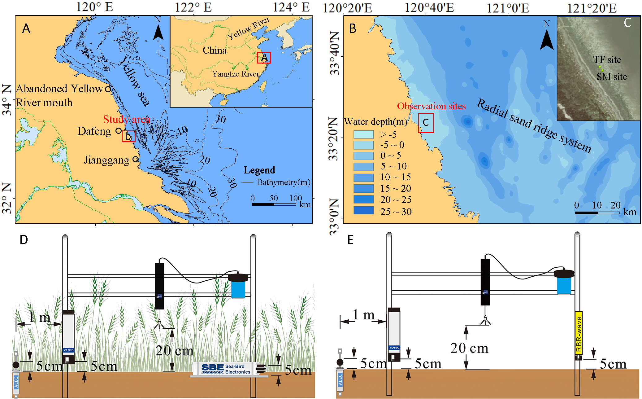
Figure 1 Location of the Doulonggang intertidal flat (A, B) enlarged view of the area (red box), (C) zoomed-in view showing the location of observation sites, (D) instruments deployed at SM site (ADV, OBS, EMCM, SBE26plus), (E) instruments deployed at TF site (ADV, OBS, EMCM, RBR-solo D).

The surficial sediments on the tidal flat become finer landward, dominated by silt and fine sand. The exotic plant Spartina alterniflora occupies the upper tidal flat (elevation above 0.4 m). The SM site was situated within the vegetated areas while the TF site was within the unvegetated areas. The distance between the two sites was around 22 m. No distinct tidal creeks were observed in the upper tidal flat.

3 Methods

3.1 Field data collection

The field observation was conducted from November 6^th to November 15^th, 2018, and all in situ measurements were synchronized at both sites. Acoustic Doppler Velocimeters (6.0 MHz vector current meter, Nortek AS, Norway) were deployed in a down-looking configuration with the transmit transducer to measure 3D velocity at 16 Hz for 256 sec every burst (4096 points per 5-min time series). The ADV probe was installed at a height of 20 cm above the seabed, and the intratidal bed-level changes were indicated by the distance between the probe and the bed surface recorded by the ADV. The accuracy of bed-level changes was ±1 mm based on laboratory tests in previous studies (Hosseini et al., 2006; Shi et al., 2015; Shi et al., 2017b). To capture the hydrodynamics during extremely shallow water stages, an electromagnetic current meter (EMCM) was used because this instrument can precisely measure velocity within a small volume using a small probe (diameter of ~3 cm). To measure the 2D near-bed current velocity for extremely shallow water conditions, the EMCM was deployed at a height of 0.05 m above the bed and operated at a burst period of 30 s and sampling frequency of 2 Hz (Figures 1D, E).

Wave parameters such as wave height and wave period were measured using self-logging sensors, including the SBE-26plus Seagauge (Sea-Bird Electronics, Washington, USA) and RBRsolo |wave (RBR Ltd., Ottawa, Canada). The instruments were horizontally placed on the sediment surface, with their pressure sensors located 5 cm above the bed surface (Figures 1D, E). To obtain high-frequency water level measurements, the pressure data were recorded at 4 Hz for a duration of 256 seconds, resulting in a total of 1024 measurements per burst.

The optical backscatter (OBS) sensors (OBS-3A, D&A Instrument Company, Washington, USA) were used to measure turbidity in the water column every five minutes. The probe of OBS was positioned 5 cm above the bed surface. The suspended sediment concentration (SSC) values were obtained by converting the turbidity values measured by the OBSs through calibration using in situ water samples (Figure 2).

FIGURE 2

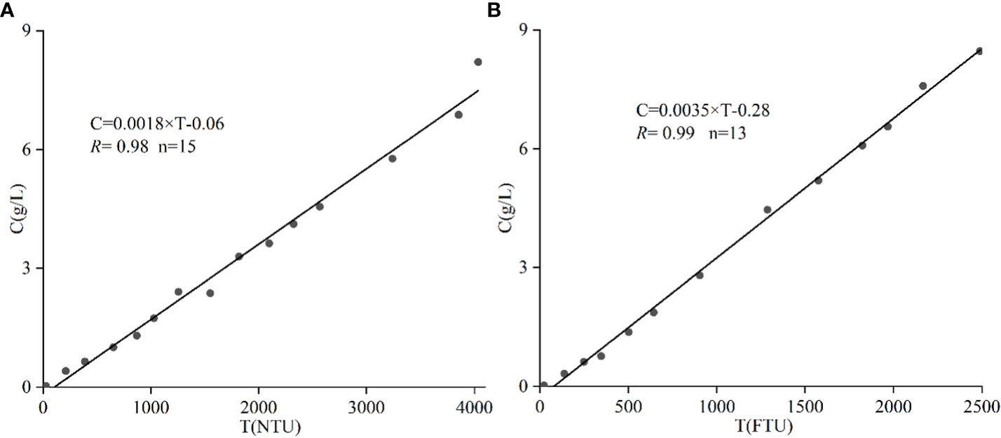
Figure 2 Calibration curves used to convert optical turbidity (T; NTU) recorded by OBSs to suspended sediment concentration (SSC) (C; g/L). (A) calibration curves for the TF site; (B) calibration curves for the SM site.

3.2 Data processing and calculation

3.2.1 Calculation of bed shear stress

The bed shear stress is a critical parameter controlling the erosion and deposition of sediments. The total bed shear stress due to waves and currents ( ${\tau }_{cw}$, $\text{N}/m^2$) is derived from the components of bed shear stress due to waves alone ( ${\tau }_w$, $\text{N}/m^2$) and currents alone ( ${\tau }_c$, $\text{N}/m^2$).

The shear stress generated by waves is closely related to the wave orbital velocity ( $U_w$, m/s). When waves propagate onto the tidal flat, they are transformed due to local topography. The wave orbital velocity is calculated using the high-frequency velocity recorded by the ADV (Wiberg and Sherwood, 2008).

$\begin{array}{ll}{\text{U}}_w=\sqrt{2{\displaystyle \sum _i{S}_{uv,i}\Delta f}}& (1)\end{array}$

where $S_{uv}=S_{uu}+S_{vv}$ is the combined horizontal spectrum of eastern and northern velocity. This method removes the influence of turbulence on wave parameters, thereby eliminating the overestimation of orbital velocity that would be induced by using the linear wave theory (Xiong et al., 2018).

However, the ADV probes were exposed to air and stopped working during extremely shallow water stages when the water depth was<0.2 m. Therefore, we used the SBE-26plus Seagage and RBRsolo | wave to observe waves during shallow water stages applying the linear wave theory, expressed as follows:

$\begin{array}{ll}{U}_w=\frac{\pi H}{Tsinh(2\pi h/L)}& (2)\end{array}$

where $H(m)$ is the wave height, $T(s)$ is the wave period, $L(m)$($=(\frac{g{T}^2}{2\pi })\tanh (\frac{2\pi h}{L})$) is the wavelength, $g(=9.8 m/s^2)$ is the gravity acceleration, and $h(m)$ is water depth.

The bed shear stress induced by waves ( ${\tau }_w)$ can be calculated from wave parameters as (Soulsby, 1995):

$\begin{array}{ll}{\tau }_w=\frac{1}{2}\rho f_w{\text{U}}_w^2& (3)\end{array}$

where $\text{ρ}$ is the fluid density (= 1030 kg/m³), $f_w$ is the wave friction factor which depends on the hydraulic regime. $f_w$ can be calculated as follows (Soulsby, 1997):

$\begin{array}{ll}{f}_w=\{\begin{array}{c}2R_w^{-0.5}, R_w\le {10}^5 (\text{laminar flow})\\ 0.0521R_w^{-0.187}, R_w>{10}^5 (\text{smooth turbulent})\\ 0.237r^{-0.52}, (\text{rough turbulent})\end{array}& (4)\end{array}$

where $R_w(=\frac{U_{w}A}{\nu })$ is the wave Reynolds number, $r (=\frac{A}{k_s})$ is the relative roughness, $\text{v}(\text{m}/\text{s})$ is the kinematic viscosity of seawater, A (= $\frac{U_{W}T}{2\pi },m$) is the semi-orbital excursion, and $k_s$ (= $2.5d_{50}$, $d_{50}$ is the median grain size) is the Nikuradse roughness (Fredsøe, 1984).

The bed shear stress induced by current ( ${\tau }_c)$ is calculated from friction velocity ( $u_{*}$) (Soulsby, 1995):

$\begin{array}{ll}{\tau }_c={\rho }_w{u}_{*}^2& (5)\end{array}$

The logarithmic velocity profile (LP method) is used to describe the velocity structure in the bottom boundary layer within a weak hydrodynamic environment (Soulsby and Dyer, 1981; Grant and Madsen, 1986; Shi et al., 2019), expressed as (Dyer, 1986; Whitehouse et al., 1999)

$\begin{array}{ll}u=\frac{u_{*}}{k}\text{ln}(\frac{z}{z_0})& (6)\end{array}$

where $u(m/s)$ is the velocity at height z $(m)$ above the bed, measured by EMCM during extremely shallow water stages and ADV during deep water stages. $K(=0.4)$ is the von Karman’s constant, and $Z_0(=\frac{k_s}{30},m)$ is the bed roughness length related to the Nikuradse grain roughness (Whitehouse et al., 1999).

The bed shear stress due to the combined action of waves and currents ( ${\tau }_{cw}$) is determined using the proposed models by Soulsby and Clarke (2005), expressed as:

$\begin{array}{ll}{\tau }_{cw}=\sqrt{{({\tau }_m+{\tau }_w\left|cos{\phi }_{cw}\right|)}^2+{({\tau }_w\left|sin{\phi }_{cw}\right|)}^2}& (7)\end{array}$

where ${\phi }_{cw}$ is the angle between waves and currents, and the average total shear stress ${\tau }_m$ is calculated as:

$\begin{array}{ll}{\tau }_m={\tau }_c[1+1.2{(\frac{{\tau }_w}{{\tau }_c+{\tau }_w})}^{3.2}]& (8)\end{array}$

3.2.2 Cumulative bed level changes during extremely shallow water stages

The cumulative bed level changes of extremely shallow water stages for two consecutive tidal cycles were obtained using the following method:

$\begin{array}{ll}\text{Δ}{D}_{i\_\text{shallow }}=D_{i\_end}–D_{i+1\_initial}& (9)\end{array}$

where $D_{i_{end}}(mm)$ is the relative distance between the ADV probe and the bed surface at the last effective burst during the ebb tide stage, $D_{i+1\_initial}$ is the distance between the ADV probe and the bed surface for the first effective burst of the next tide. A positive value indicates deposition and a negative value indicates erosion.

3.2.3 Critical shear stress for erosion ( ${\tau }_{ce}$)

The critical shear stress for erosion ( ${\tau }_{ce}$) was estimated following the approach recommended by Andersen et al. (2007) and Shi et al. (2015), which has been validated in tidal flat environments. According to their theory, the values of ${\tau }_{cw}$ recorded at the point of erosion initiation (i.e., when there was an noticeable decrease in bed level elevation and a significant increase in SSC) are considered as the critical shear stress for erosion ( ${\tau }_{ce}$).

The bed level started to drop during the flooding tide of T3 when ${\tau }_{cw}$ reached a high value of 0.24 $\text{N}/m^2$ (Figures 3D, F) at the TF site, whereas at the SM site, erosion started when ${\tau }_{cw}$ was about 0.17 $\text{N}/m^2$ during the flooding tide of T9 (Figures 3D, F), as determined from the bed-level changes obtained using the high-resolution ADV. These values (0.24 and 0.17 $\text{N}/m^2$) are considered as the ${\tau }_{ce}$ values for the TF and SM sites, respectively.

FIGURE 3

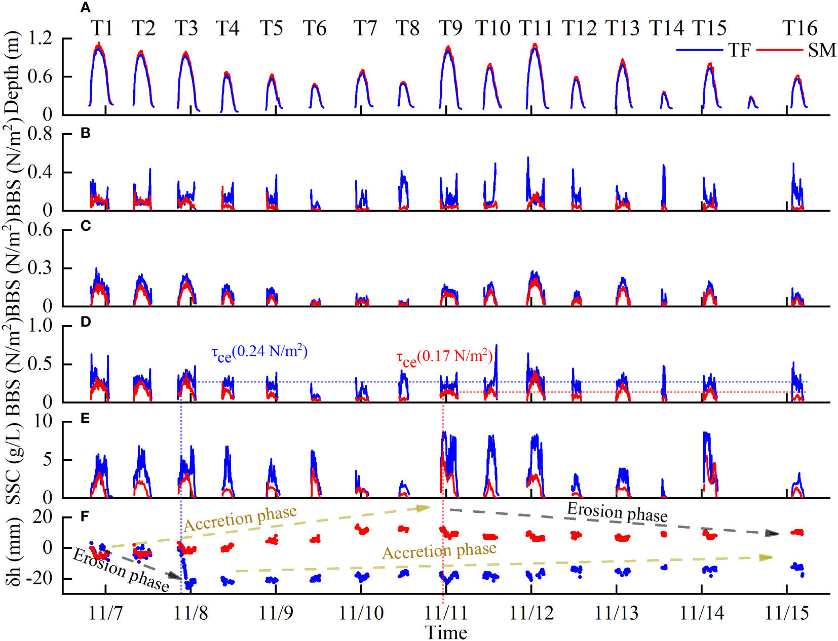
Figure 3 Time series of (A) water depth, (B) bed shear stress due to currents ( ${\tau }_c$); (C) bed shear stress due to waves ( ${\tau }_w$); (D) bed shear stress due to currents and waves ( ${\tau }_{cw}$); (E) suspended sediment concentration (SSC); (F) bed level changes (positive value represents deposition, the negative value represents erosion, and the single point represents the value of each burst.

3.2.4 Index of agreement

The Index of agreement ( $I_{ndex}$) is often used to evaluate the difference between the same physical quantity from two different methods by showing the degree of similarity quantitatively:

$\begin{array}{ll}{I}_{ndex}=1-\frac{{\sum }^{}{(x-\overline{y})}^2}{{\sum }^{}{(\left|x-\overline{y}\right|+\left|y-\overline{y}\right|)}^2}& (10)\end{array}$

Where x and y are the two datasets involved in the comparison, and the $I_{ndex}$ ranges from 0 to 1. The larger the value of the $I_{ndex}$, the higher the degree of similarity between the two datasets. $I_{ndex}$ =1 indicates that the two datasets are completely consistent. In this study, the index of agreement is used to compare the wave orbital velocity calculated using different methods.

4 Results

4.1 Hydrodynamics

During our field measurements, wind patterns showed significant temporal variations at both sites, which were classified into two periods. The first period, composed of T1~T3 and T9~T11, was characterized by strong northerly onshore winds with speeds ranging from 3.4 to 10.5 m/s and averaging at 7.6 m/s (Figure 4A). These relatively strong onshore winds generated large waves, and the average significant wave height reached a maximum of 0.43 m and 0.33 m at the two sites. The average significant wave heights during extremely shallow water stages were 0.03 m and 0.05 m at the SM and TF sites, respectively (Figure 4C). The tide-average maximum significant wave height was 0.27 m at the SM site, 25% lower than that at the TF site (0.36 m) due to the damping effect of vegetation.

FIGURE 4

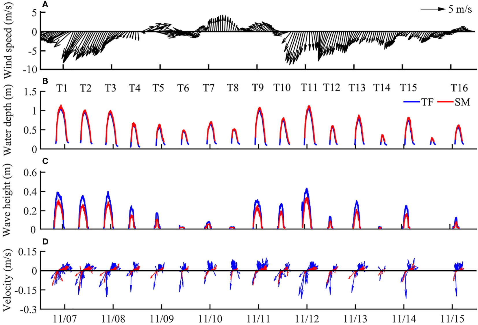
Figure 4 Time series of (A) wind speed and direction. Wind data were recorded every hour; (B) water depth; (C) significant wave height; (D) current velocity at the TF, and the SM sites.

The second period, composed of T4~T8 and T12~T16, was characterized by relatively weak winds ranging from 0.85~8.6 m/s, with an average of 4.6 m/s. During this period, the tide-averaged maximum wave heights were much lower, with an average of 0.12 m and 0.19 m at the SM and TF sites, respectively. Since wave height was limited by water depth in tidal flat environments (Figure 3A), the average significant wave heights during extremely shallow water stages were 0.02 m and 0.03 m at the SM and TF sites, respectively (Figure 4C).

The tidal current near the bottom (at the height of 0.05 m above the bed) at both sites was characterized by a rotational flow pattern (Figure 4D). High current velocities normally occurred during the flood stages of extremely shallow water stages, followed by low velocities during deep water stages, and the minimum current speed occurred during slack water. At the SM site, the tide-averaged current velocity near the bed during extremely shallow water stages ranged from 0.01 to 0.22 m/s (average value of 0.05 m/s), which was much higher than that during deep water stages (0.01–0.09 m/s; the average value of 0.02 m/s). Similarly, the velocities at the TF site during extremely shallow water stages (ranging from 0.01 to 0.29 m/s with an average of 0.06 m/s) were higher than those during deep water stages (ranging from 0.01 to 0.23 m/s with an average of 0.05 m/s).

4.2 Erosion and accretion processes

4.2.1 Shear stress

The wave orbital velocity calculated by the two different methods were shown in Figure 5. Linear wave theory was used to calculate $U_w$ using the data recorded by the SBE26plus and RBRsolo |wave, while the spectral method was used to estimate $U_w$ using ADV recorded data. For both sites, the time series of $U_w$ obtained using different methods show similar variation patterns during tidal cycles. At the SM site, the two methods provide close $U_w$ values with an $I_{ndex}$ value reaching 0.91(Table 1). However, at the TF site, agreement in the magnitude of $U_w$ is weaker. The Uw values calculated from the two methods were more deviant during deep water stages than during shallow water stages ( $I_{ndex}$ = 0.75), demonstrating that the two methods produce more consistent results in shallow water environments. For convenience, the spectral method is used in the calculation of $U_w$, except during extremely shallow water stages when ADV stopped working and the linear wave theory is used.

FIGURE 5

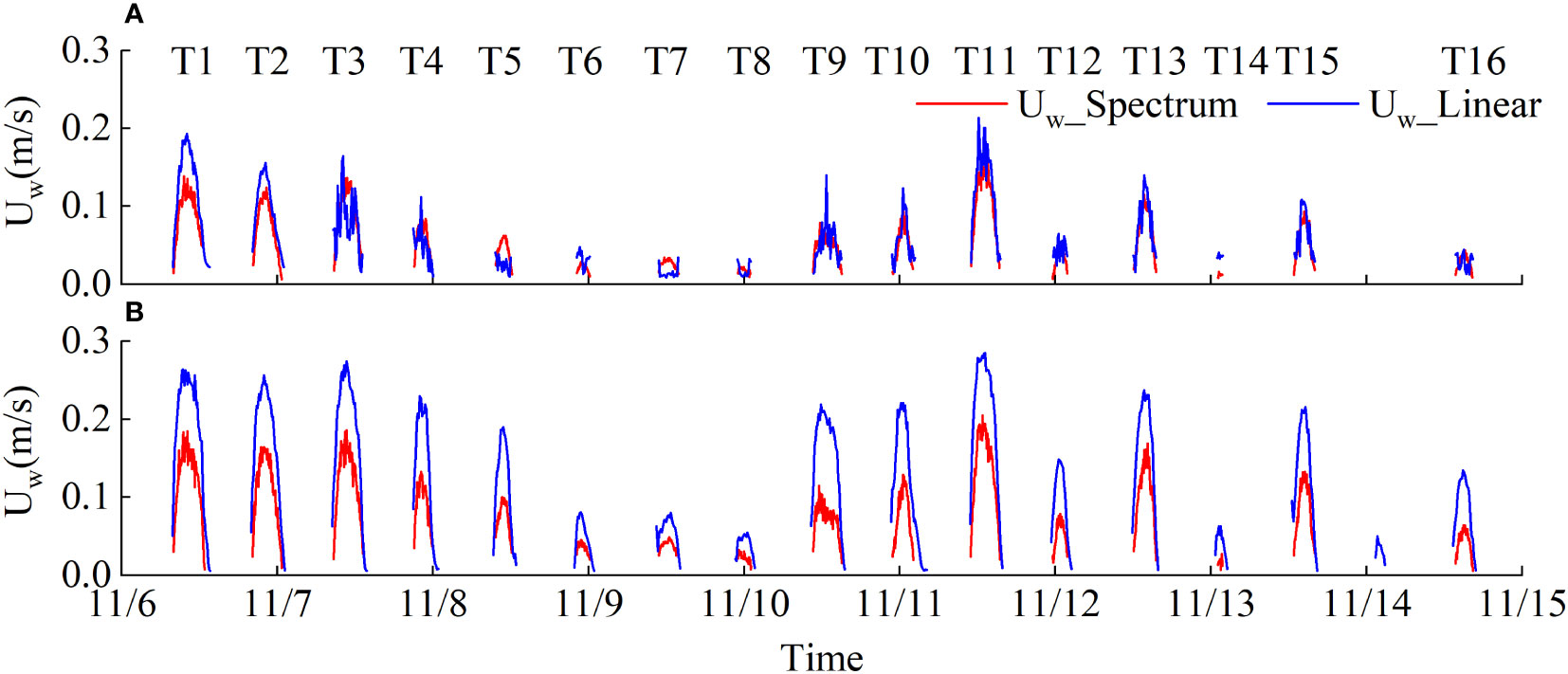
Figure 5 Time-series of (A) wave orbital velocity calculated by different methods at the SM site (B) wave orbital velocity calculated by different methods at the TF site.

TABLE 1

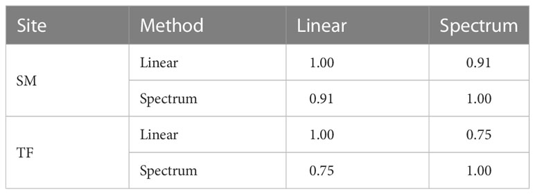
Table 1 I_ndex of agreement for wave orbital velocity using different methods.

The values of ${\tau }_c$, ${\tau }_w$ and ${\tau }_{cw}$ are shown in Figures 3B–D and statistically summarized in Tables 2, 3. Generally speaking, for all tidal cycles, the average values of ${\tau }_c$ during flood tides (0.06 $\text{N}/m^2$) in extremely shallow water stages were higher than those in ebb tides (0.02 $\text{N}/m^2$) and those in deep water stages because of the flood surge (Zhang et al., 2021) at the SM site. The differences in ${\tau }_c$ were more pronounced on the unvegetated mudflat. The average value during shallow water stages in flood tides (0.18 $\text{N}/m^2$) was six times higher than that in ebb tides (0.03 $\text{N}/m^2$) and slightly higher than that in deep water stages (0.15 $\text{N}/m^2$). The ${\tau }_w$ values during extremely shallow water stages were very small due to the shallow water environment. The average values during deep water stages (0.10 $\text{N}/m^2$ at TF site, 0.07 $\text{N}/m^2$ at SM site) were two times higher than those during extremely shallow water stages (0.05 $\text{N}/m^2$ at TF site, 0.03 $\text{N}/m^2$ at SM site).

TABLE 2

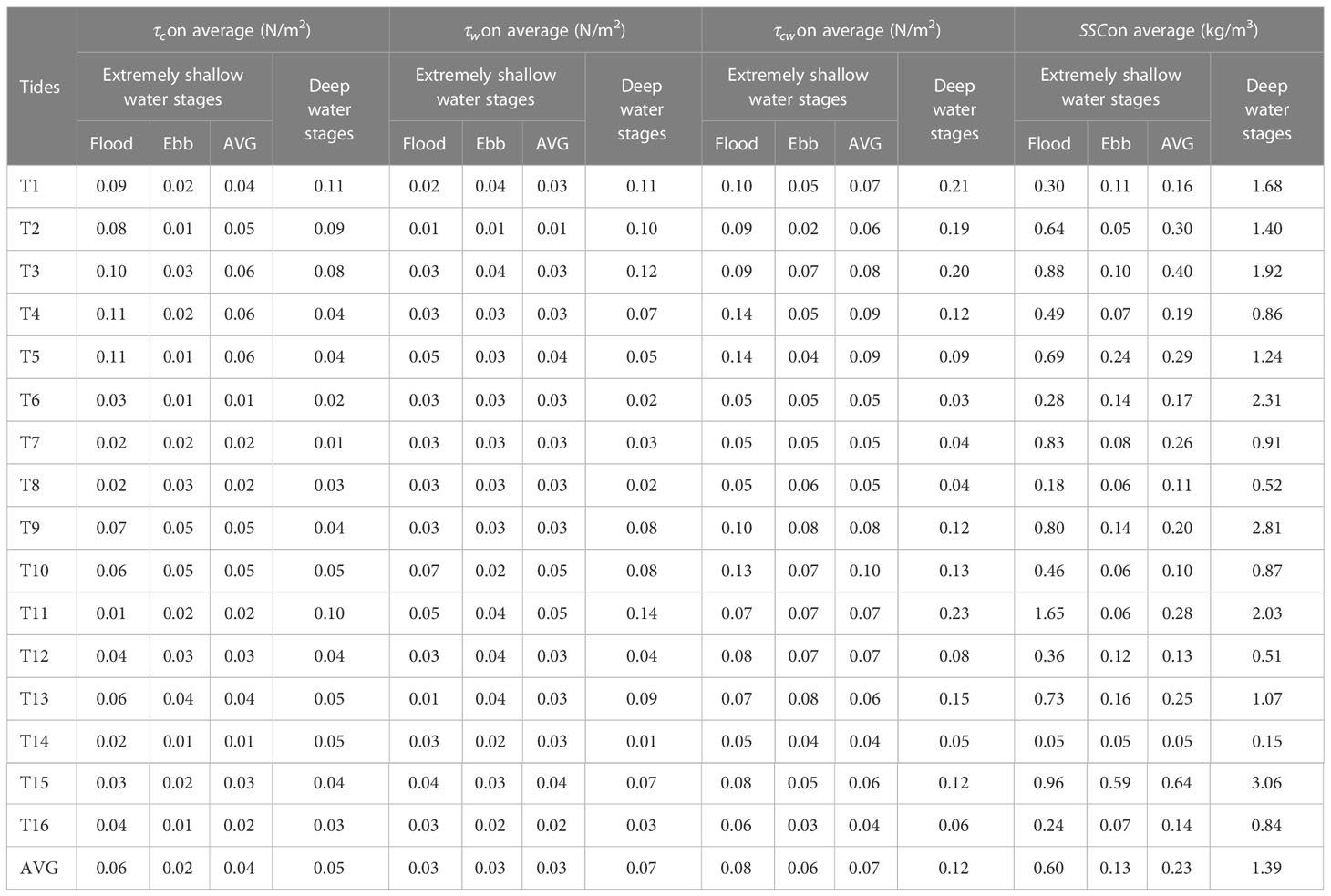
Table 2 Comparison of bed shear stress due to waves ( ${\tau }_w$), currents ( ${\tau }_c$), and combined current–wave action ( ${\tau }_{cw}$), and SSC at water depths (h) of<0.2m (Extremely Shallow Water Stages) and >0.2m (deep water stages) at the SM site.

TABLE 3

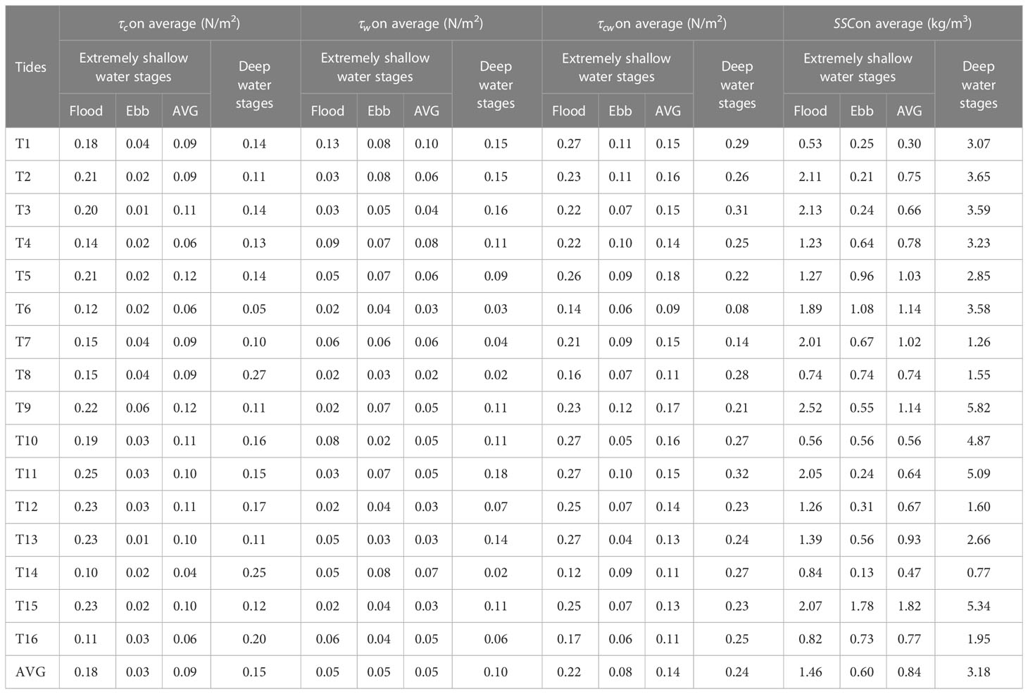
Table 3 Comparison of bed shear stress due to waves ( ${\tau }_w$), currents ( ${\tau }_c$), and combined current–wave action ( ${\tau }_{cw}$), and SSC at water depths (h) of<0.2m (Extremely Shallow Water Stages) and >0.2m (deep water stages) at the TF site.

The maximum ${\tau }_{cw}$ within a tidal cycle usually appeared during deep water stages (Figure 3D), which was much larger than that during extremely shallow water stages. Correspondingly, the average ${\tau }_{cw}$ during the flood stages (0.22 $\text{N}/m^2$ at TF site, 0.08 $\text{N}/m^2$ at SM site) and ebb stages (0.08 $\text{N}/m^2$ at TF site, 0.06 $\text{N}/m^2$ at SM site) during extremely shallow water stages was much lower than the ${\tau }_{ce}$ values (0.24 $\text{N}/m^2$ at TF site, 0.17 $\text{N}/m^2$ at SM site). Therefore, effective resuspension cannot be initiated.

4.2.2 Suspended sediment concentration

The SSC near the bed had a similar temporal variation pattern to ${\tau }_{cw}$ (Figures 3D, E), with peak values usually occurring at the highest water level. The average SSC during flood stages was greater than that during ebb stages. The average SSC during deep water stages (3.18 $\text{kg}/m^3$ at the TF site, 1.39 $\text{kg}/m^3$ at the SM site) was much higher than that during extremely shallow water stages at both sites (Figure 3E; Tables 2, 3).

4.2.3 Duration of extremely shallow water stages and deep water stages

Due to continuous emergence and submergence, salt marshes experience temporal-spatial variations in water depth, leading to the frequent occurrence of extremely shallow water conditions (twice every tide). Compared with the relatively long duration of the deep water stages (224 min at the TF site, 233 min at the SM site), the duration of extremely shallow water tides during the flood tides (10 min at the TF site, 9 min at the SM site) was only half of that during the corresponding ebb stages (19 min at the TF site, 23 min at the SM site), and the total duration of extremely shallow water stages accounted for 14~15% of the entire tidal cycle (Tables 4, 5).

TABLE 4

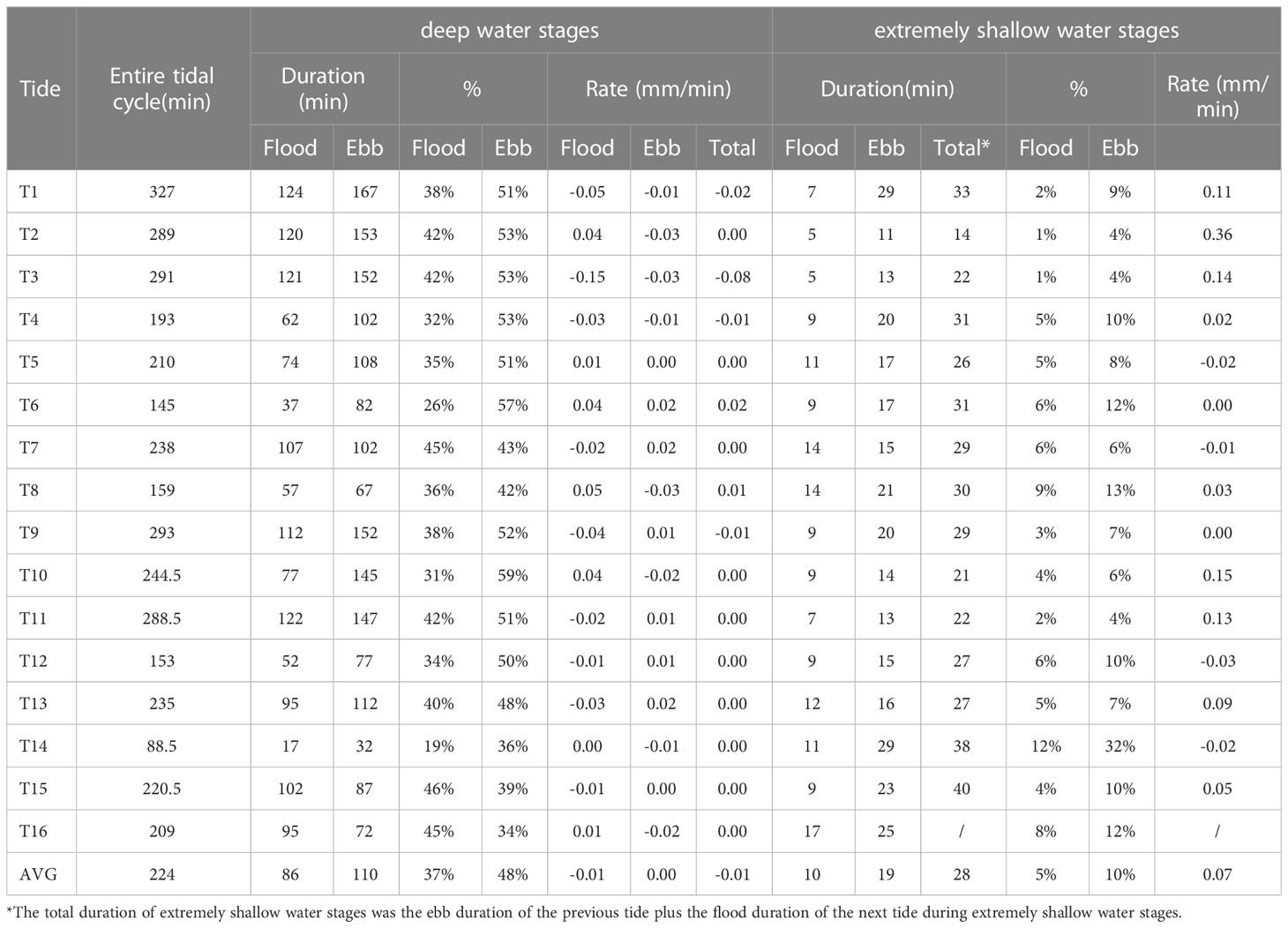
Table 4 Comparison of duration of deep (> 0.2 m) and extremely shallow water stages (< 0.2 m) within different tidal cycles and the rates of bed-level change (mm/min) for different stages at the TF site.

TABLE 5

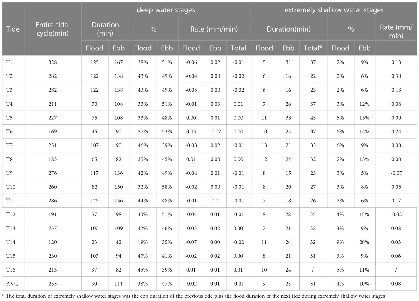
Table 5 Comparison of duration of deep (> 0.2 m) and extremely shallow water stages (< 0.2 m) within different tidal cycles and the rates of bed-level change (mm/min) for different stages at the SM site.

4.2.4 Bed level changes

The data of bed level changes measured by ADV during the period with effective data (h > 0.2 m) are shown in Figure 3F. Previous studies have shown that the high sediment concentration water layer near the seabed and fluid mud can affect the quality of data obtained from ADV measurements (Sahin et al., 2012; Mehta et al., 2014). During our observational period, fluid mud was not detected, and the high SSCs only occurred during deep water stages. The low-quality data were manually excluded to obtain high-quality realistic bed-level changes. The result showed that the measured bed level changes decreased during T1~T3, which was defined as the ‘erosion phase’ and then increased slowly, defined as the ‘accretion phase’ for the back-siltation during T4~T16 at the TF site. At the SM site, deposition dominated during T1–T8, and erosion occurred continuously from T9 to T16. The cumulative vertical bed-level change was +11.5 mm at the SM site and -13.5 mm at the TF site at the end of T16.

Accumulation occurred during extremely shallow water stages with a total deposition amount of +33.8 mm at the SM site and +20.8 mm at the TF site with an average bed-level change rate of 0.08 mm/min at the SM site and 0.07 mm/min at the TF site. On the other hand, erosion dominated the two sites during deep water stages, with a total erosion thickness of -22.3 mm at the SM site and -32.7 mm at the TF site with an average bed-level change rate of -0.01 mm/min at both sites.

Wind also had a significant impact on determining the deposition rate during extremely shallow water stages. Strong wind induced high waves and faster current speeds, moving more sediment to the upper flat zone. Our observation showed that the tide cycle-averaged deposition during the strong wind period was + 3.1 mm at the SM site and + 2.9 mm at the TF site, respectively. This was several times higher than that during the calm weather period (+ 1.7 mm at the SM site and + 0.4 mm at the TF site, respectively) during extremely shallow water stages. The average bed-level deposition rate reached +0.15 mm/min at the SM site and +0.12 mm/min at the TF site during the strong wind period, much higher than that during the calm weather period (+0.05 mm/min at the SM site and +0.01 mm/min at the TF site).

5 Discussion

5.1 Geomorphological changes during extremely shallow water stages in salt marshes

Tidal current and corresponding sediment transport patterns have shaped the unique geomorphic features of the mudflat. In previous studies, surges at the beginning of the flood period were as large as tens of centimeters per second (Gao, 2010; Shi et al., 2019; Zhang et al., 2021), leading to large values of bed shear stress (reaching 1.5 N/m² at the beginning of the flood tide) (Zhang et al., 2016a), which is an order of magnitude higher than the critical shear stress found on intertidal flats. Such a phenomenon also occurred in our study area. A monitoring site (CT02) was set seawards in the intertidal zone, which was 600 m away from the SM and TF site. When the tidal flat was exposed to the air, a ruler was used to measure the distance between the ADV and seabed (the red points in Figure 6E) to reflect the erosion and accretion results during the extremely shallow water stage at the CT02 site. As shown in Figure 6, surges were commonly observed during extremely shallow water stages. Affected by the high flow velocity (0.2 m/s), the shear stress greatly increased, with an average value of 0.42 N/m² during the flood tide. The short-term strong hydrodynamics led to a large volume of bottom sediment resuspension, and the SSC reached the first peak, accompanied by strong erosion fluxes with an average magnitude of -21.9 mm per tide. These results were similar to those of previous studies (Xu et al., 1994; Gao, 2010; Hughes, 2012; Zhang et al., 2016a; Shi et al., 2019).

FIGURE 6

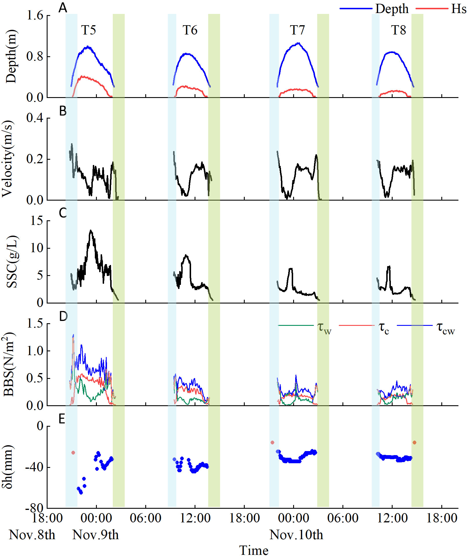
Figure 6 Time series of hydrodynamics and sediment transport-related parameters at site CT02 (A) water depth and significant wave height, (B) current velocity, (C) suspended sediment concentration (SSC), (D) bed shear stress due to currents ( ${\tau }_c$), waves ( ${\tau }_w$), and current and wave interactions ( ${\tau }_{cw}$); (E) bed level changes (the first point in T1 was set to zero), blue bars indicate the flood tide during extremely shallow water stages, and green bars indicate the ebb tide during extremely shallow water stages.

However, the mechanism by which the surge was formed and how it influences sediment transport in the salt marsh was still uncovered, where hydrodynamic characters were quite different from those on the mudflat. The existence of vegetation increases surface roughness, reduces flow velocity, and influences the generation of turbulence and energy dissipation, weakening the hydrodynamic force within the salt marsh (Leonard and Luther, 1995; Leonard et al., 2002; Neumeier and Ciavola, 2004; Neumeier and Amos, 2006). In this study, the flood tide was relatively slow when it propagated to the salt marsh, and the flow velocity was only 0.05 m/s in the vegetated areas and 0.06 m/s in the unvegetated areas during extremely shallow water stages. Breaking water was not observed at those sites. Additionally, limited by the shallow water depth, waves were very small, resulting in very weak hydrodynamic force during extremely shallow water stages. As a result, the mean ${\tau }_{cw}$ value ranged from 0.04~0.1 $\text{N}/m^2$ in the vegetated areas and 0.09~0.18 $\text{N}/m^2$ in neighboring unvegetated areas, much lower than the critical bed shear stress (0.24 $\text{N}/m^2$ in the unvegetated areas and 0.17 $\text{N}/m^2$ in neighboring vegetated areas). Therefore, the tidal front water was too weak to generate effective resuspension, and the local sediments in the salt marsh were not stirred at this stage. Meanwhile, the tidal front water with high SSC, caused by sediment erosion of the lower tidal flat, was carried to the upper flat along the tidal flat profile (Gao, 2010). In this area, the low-sloped morphology and vegetation lead to high bed resistance, causing the settling of suspended sediment and a decrease in suspended sediment concentration during this period. These sediments deposited in the salt marsh with a mean value of 2.3 mm per tide and 1.4 mm per tide in the unvegetated areas during extremely shallow water stages (Table 6), and the water column was relatively clear for a short period. Compared with the unvegetated areas, the vegetated areas had a higher flow reduction rate and sediment capture effectiveness (Leonard and Croft, 2006; Yang and Nepf, 2019; Chen et al., 2020), resulting in more deposition. The cumulative net deposition thickness during extremely shallow water stages of the whole tidal cycle in the vegetated areas was + 33.8 mm and + 20.8 mm in the unvegetated areas.

TABLE 6

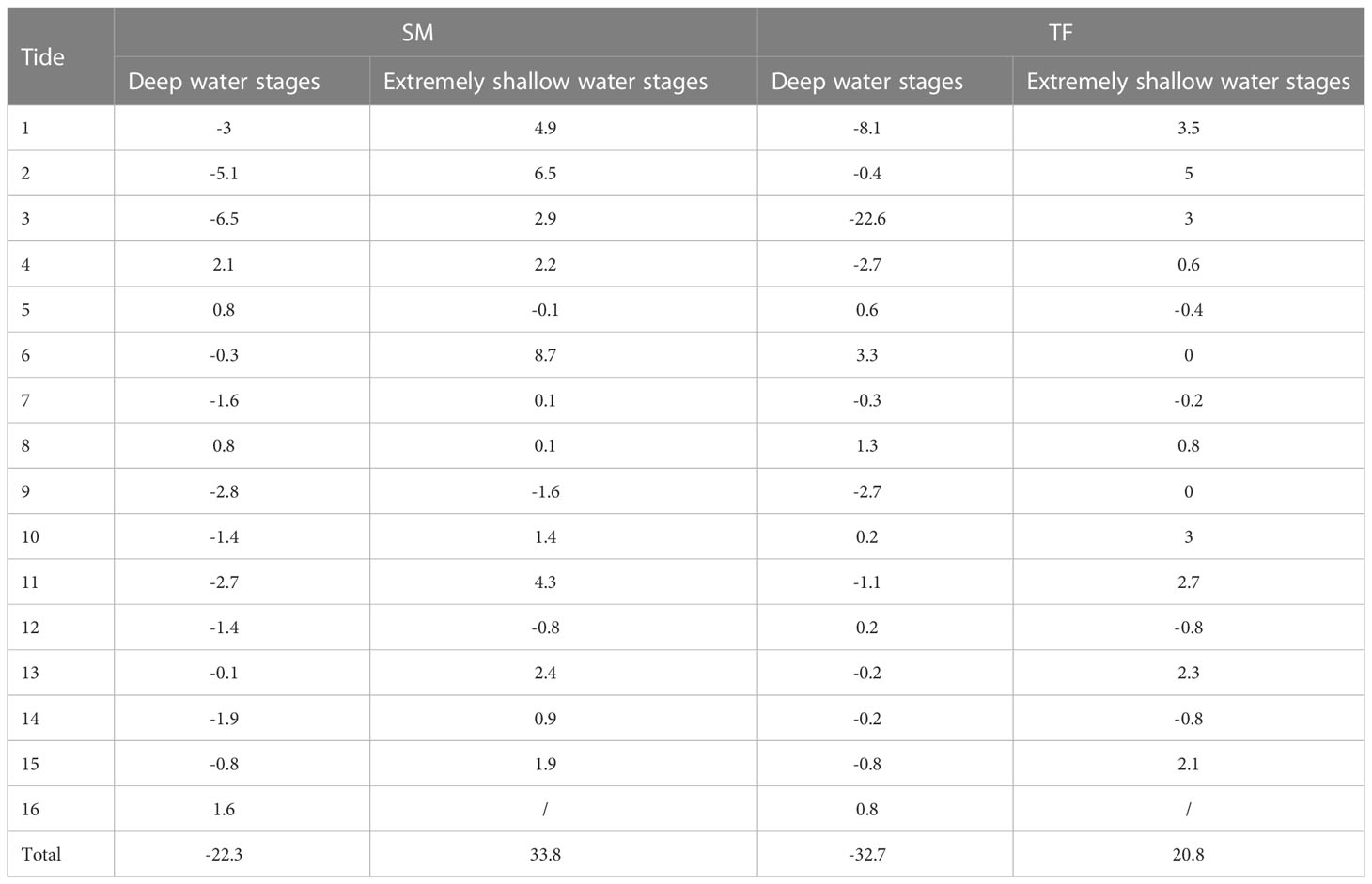
Table 6 Statistics of the bed level changes (unit: mm) at the TF and the SM sites.

After the extremely shallow water stage, flooding tides and waves became stronger, and ${\tau }_w$ greatly increased to a mean value of 0.07 $\text{N}/m^2$ (vegetated areas) and 0.10 $\text{N}/m^2$ (unvegetated areas) during the deep water stages of different tidal cycles (Tables 2, 3). The mean ${\tau }_{cw}$ also increased to higher values ranging between 0.05 to 0.23 $\text{N}/m^2$ (vegetated areas) and 0.09~0.32 $\text{N}/m^2$ (unvegetated areas), exceeding the local critical bed shear stress and causing strong sediment resuspension. Accordingly, SSC increased (Figure 3E), and sediment was transported away by tidal currents. Erosion was more obvious in the unvegetated areas because of the relatively strong hydrodynamic force and lack of vegetation protection. Our results showed that the net erosion amount during deep water stages was -32.7 mm in the unvegetated areas and -22.3 mm in the vegetated areas. The distinct sediment dynamics between the two sites resulted in a net deposition in the vegetated areas and net erosion in the unvegetated areas, thus influencing the morphological evolution of the tidal flat system.

Although the duration of extremely shallow water stages in the salt marsh was only a few minutes, accounting for about 14-15% of the whole tidal cycle, the rate of bed level changes during these stages was 7~8 times greater than that during deep water stages at both sites. This resulted in a profound impact on sediment transport, highlighting the importance of extremely shallow water stages in the replenishment of sediments and the maintenance of salt marshes.

Strong winds can significantly contribute to the development of salt marshes (French and Spencer, 1993; Schuerch et al., 2013), according to previous studies. Storms can generate strong waves in a short period of time and directly affect the front of the tidal flat. This process is crucial for understanding the long-term morphological evolution mechanism of salt marshes in high-turbidity intertidal zone. Abundant sediments are brought into the salt marsh from the subtidal zone under the influence of strong onshore winds during extremely shallow water stages. Vegetation causes sediment adhesion and deposition (Shi et al., 2000; Leonard and Croft, 2006), and the average SSC increased from 1.35 g/L (during calm weather) to 1.65 g/L (during rough weather) in unvegetated areas, while it increased from 0.48 g/L to 0.79 g/L in the vegetated areas during extremely shallow water stages in the initial flood stages (Figure 3E). Consequently, the average bed level changes rate reached +0.15 mm/min in the vegetated areas and +0.12 mm/min in the unvegetated areas, much higher than that during calm weather. Our results indicate that weather conditions are also crucial factors in determining sediment transport patterns within salt marshes during extremely shallow water stages.

5.2 Linking extremely shallow water stages with microtopography in salt marshes

Many studies have found that the formation of ripples is the result of local turbulence occurring at the interface between the seabed and water (Coleman and Melville, 1994; Bartholdy et al., 2005; Bose and Dey, 2012). Previous field observations showed a high erosion rate and strong turbulence lead to an increase in ripple height, which can cause the formation of microtopography, such as sand ripples and grooves (Zhang et al., 2016a), and further promote the formation of large geomorphic units, such as tidal creek (Zhou et al., 2014). During our observations, sand ripples approximately 1-2 cm in height and 5-10 cm in length were found on the tidal flat. The wave crest can be flattened by the sheet flow (Gao, 2010) and evolved into a ‘flat bed’, which may occur during extremely shallow water stages.

In this study, the salt marsh was observed to be dominated by strong accumulation during extremely shallow water stages, resulting in a lack of ripples at the two sites. Abundant accumulation filled the wave trough, and the relatively strong deposition rate and weak turbulence led to a reduction in ripple height (Shi et al., 2017a). Therefore, the topography was relatively flat in the observed salt marsh area (Figure 7). Additionally, salt marshes reduced the resuspension rate of sediment by decreasing flow velocity and stabilizing sediment. The surface sediment within 10 cm was re-mixed by the burrowing organisms within 4 to 6 hours, thereby also flattening current-formed ripple patterns. Overall, the hydrodynamic processes within salt marshes during extremely shallow water stages limit the generation of micro topography.

FIGURE 7

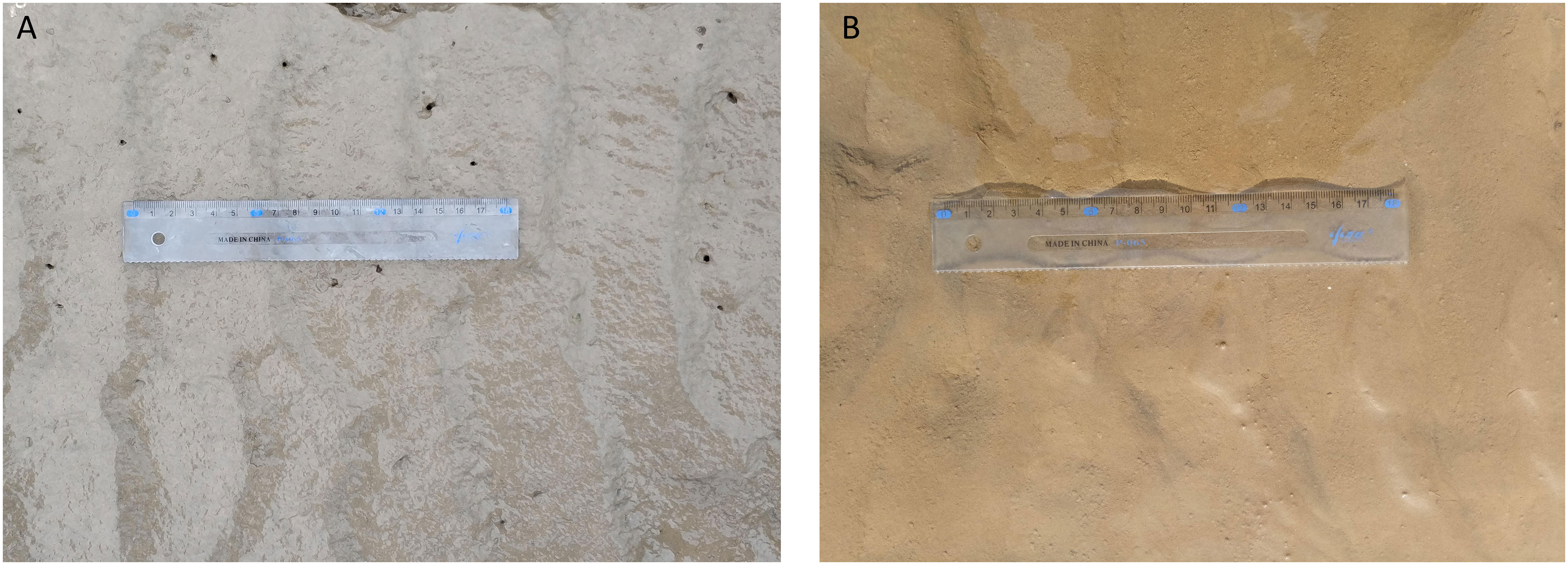
Figure 7 Photographs of ripples at the (A) SM site and (B) TF site.

As discussed above, strong deposition occurred during extremely shallow water stages, while erosion occurred during deep water stages in salt marshes, resulting in significant bed-level changes. We conclude that although extremely shallow water stages are transient, this period substantially influences sediment transport within tidal cycles, and plays a significant role in the formation and evolution of microtopography on tidal flats.

6 Conclusions

Extremely shallow water stages had an important impact on the maintenance of salt marshes by inducing significant sediment accretion in vegetated areas. This study explored the morphological dynamics and quantified the sediment erosion–accretion processes during extremely shallow water stages through integrated near-bed field measurements within salt marshes. The main conclusions are as follows:

(1) Current and wave induced shear stress was less than the critical shear stress for erosion ( ${\tau }_{ce}$) during extremely shallow water stages but larger than ${\tau }_{ce}$ during deep water stages. These changes led to deposition during extremely shallow water stages and erosion during deep water stages in almost all observed tidal cycles. In addition, gradual accumulation processes played a very important role in replenishing sediments in salt marshes.

(2) The deposition rate was more significant under windy weather during extremely shallow water stages. The average bed level changes rate reached +0.15 mm/min in the vegetated areas and +0.12 mm/min in the unvegetated areas, much higher than that during calm weather (+0.05 mm/min in the vegetated areas and +0.01 mm/min in unvegetated areas).

(3) Although extremely shallow water stages made up only 14~15% of the entire tidal cycle, the tide-average bed level change rate during extremely shallow water stages was 7 times faster than that during deep water stages.

(4) The deposition during extremely shallow water stages filled the wave trough, resulting in the relatively flat topography in salt marsh and restricting the generation of microtopography within salt marshes.

Data availability statement

The original contributions presented in the study are included in the article/supplementary material. Further inquiries can be directed to the corresponding authors.

Author contributions

The contributions made by each of the authors are listed as follows: 1) YW & FX put forward the idea, designed the experiments and funded the study. 2) DC processed the main measurements/experiments data and completed the major sections of the manuscript. 3) JT helped processing data. 4) JC, ML,YZ & BS reviewed this article and made suggestions to improve it. All authors contributed to the article and approved the submitted version.

Acknowledgments

This research was supported by the following grants: the Jiangsu Special Program for Science and Technology Innovation (JSZRHYKJ202106), the Youth Foundation of Guangxi Zhuang Autonomous Region (2022GXNSFBA035566), innovation Driven Development Foundation of Guangxi (AD22080035), the Young Scientists Fund of the National Natural Science Foundation of China (42006149), the Key Laboratory of Coastal Salt Marsh Ecosystems and Resources, Ministry of Natural Resources (KLCSMERMNR2021108). We thank Gao C, Pan YP, Lan TF, Lu T for their assistance in the field work and laboratory measurements.

Conflict of interest

The authors declare that the research was conducted in the absence of any commercial or financial relationships that could be construed as a potential conflict of interest.

Publisher’s note

All claims expressed in this article are solely those of the authors and do not necessarily represent those of their affiliated organizations, or those of the publisher, the editors and the reviewers. Any product that may be evaluated in this article, or claim that may be made by its manufacturer, is not guaranteed or endorsed by the publisher.

References

Allen J. R. L. (1996). Geomorphology and sedimentology of estuaries. Sedimentary Geol. 105, 110–111. doi: 10.1016/0037-0738(95)00149-2

CrossRef Full Text | Google Scholar

Allen J. R. L. (2000). Morphodynamics of Holocene salt marshes: a review sketch from the Atlantic and southern north Sea coasts of Europe. Quaternary Sci. Rev. 18, 1155–1231. doi: 10.1016/S0277-3791(99)00034-7

CrossRef Full Text | Google Scholar

Andersen T. J., Fredsoe J., Pejrup M. (2007). In situ estimation of erosion and deposition thresholds by acoustic Doppler velocimeter (ADV). Estuarine Coast. Shelf Sci. 75, 327–336. doi: 10.1016/j.ecss.2007.04.039

CrossRef Full Text | Google Scholar

Bartholdy J., Flemming B. W., Bartholomä A., Ernstsen V. B. (2005). Flow and grain size control of depth-independent simple subaqueous dunes. J. Geophysical Research: Earth Surface 110 (F4). doi: 10.1029/2004JF000183

CrossRef Full Text | Google Scholar

Bose S. K., Dey S. (2012). Instability theory of sand ripples formed by turbulent shear flows. J. Hydraulic Eng. 138, 752–756. doi: 10.1061/(ASCE)HY.1943-7900.0000524

CrossRef Full Text | Google Scholar

Cahoon D., Lynch J., Powell A. (1996). Marsh vertical accretion in a southern California estuary, U.S.A. Estuar. Coast. Shelf Sci. - Estuar. Coast. SHELF Sci. 43, 19–32. doi: 10.1006/ecss.1996.0055

CrossRef Full Text | Google Scholar

Chen D., Li M., Zhang Y., Zhang L., Tang J., Wu H., et al. (2020). Effects of diatoms on erosion and accretion processes in saltmarsh inferred from field observations of hydrodynamic and sedimentary processes. Ecohydrology 13, 2246. doi: 10.1002/eco.2246

CrossRef Full Text | Google Scholar

Coleman S. E., Melville B. W. (1994). Bed-form development. J. Hydraulic Eng. 120, 544–560. doi: 10.1061/(ASCE)0733-9429(1994)120:5(544)

CrossRef Full Text | Google Scholar

Davidson-Arnott R. G. D., van Proosdij D., Ollerhead J., Schostak L. (2002). Hydrodynamics and sedimentation in salt marshes: examples from a macrotidal marsh, bay of fundy. Geomorphology 48, 209–231. doi: 10.1016/S0169-555X(02)00182-4

CrossRef Full Text | Google Scholar

Dyer K. R. (1986). Coastal and estuarine sediment dynamics. Chichester, Sussex (UK): John Wiley Sons, 1986, 358.

Google Scholar

Fagherazzi S., Mariotti G. (2012). Mudflat runnels: evidence and importance of very shallow flows in intertidal morphodynamics. Geophysical Res. Lett. 39 (14). doi: 10.1029/2012GL052542

CrossRef Full Text | Google Scholar

Fagherazzi S., Mariotti G., Wiberg P. L., McGlathery K. J. (2013). Marsh collapse does not require Sea level rise. Oceanography 26, 70–77. doi: 10.5670/oceanog.2013.47

CrossRef Full Text | Google Scholar

Fan X., Tao J., Zeng Z., Coco G., Zhang C. (2016). Mechanisms underlying the regional morphological differences between the northern and southern radial sand ridges along the jiangsu coast, China. Mar. Geol. 371, 1–17. doi: 10.1016/j.margeo.2015.10.019

CrossRef Full Text | Google Scholar

Fredsøe J. (1984). Turbulent boundary layer in wave-current motion. J. Hydraulic Eng. 110, 1103–1120. doi: 10.1061/(ASCE)0733-9429(1984)110:8(1103)

CrossRef Full Text | Google Scholar

French J. R., Spencer T. (1993). Dynamics of sedimentation in a tide-dominated backbarrier salt marsh, Norfolk, UK. Mar. Geol. 110, 315–331. doi: 10.1016/0025-3227(93)90091-9

CrossRef Full Text | Google Scholar

Ganju N. K., Defne Z., Kirwan M. L., Fagherazzi S., D'Alpaos A., Carniello L. (2017). Spatially integrative metrics reveal hidden vulnerability of microtidal salt marshes. Nat. Commun. 8, 14156. doi: 10.1038/ncomms14156

PubMed Abstract | CrossRef Full Text | Google Scholar

Ganju N. K., Kroeger K. D., Kirwan M. L., Dickhudt P. J., Guntenspergen G. R., Cahoon D. R. (2015). Sediment transport based metrics of wetland stability. Geophysical Res. Lett. 42, 7992–8000. doi: 10.1002/2015GL065980

CrossRef Full Text | Google Scholar

Gao S. (2010). Extremely shallow water benthic boundary layer processes and the resultant sedimentological and morphological characteristic(in Chinese with English abstract). Acta Sedimentologica Sin. 28, 926–932. doi: 10.14027/j.cnki.cjxb.2010.05.005

CrossRef Full Text | Google Scholar

Grant W. D., Madsen O. S. (1986). The continental-shelf bottom boundary layer. Annu. Rev. Fluid Mechanics 18, 265–305. doi: 10.1146/annurev.fl.18.010186.001405

CrossRef Full Text | Google Scholar

Hosseini S. A., Shamsai A., Ataie-Ashtiani B. (2006). Synchronous measurements of the velocity and concentration in low density turbidity currents using an acoustic Doppler velocimeter. Flow Measurement Instrumentation 17, 59–68. doi: 10.1016/j.flowmeasinst.2005.05.002

CrossRef Full Text | Google Scholar

Hughes Z. J. (2012). Tidal channels on tidal flats and marshes. In: Davis R. Jr, Dalrymple R. (eds) Principles of Tidal Sedimentology. 269–300. doi: 10.1007/978-94-007-0123-6_11

CrossRef Full Text | Google Scholar

Jacobson H. A., Jacobson G. L. Jr. (1989). Variability of vegetation in tidal marshes of Maine, U.S.A. Can. Joumal Bot. 67 (1), 230–238. doi: 10.1139/b89-03

CrossRef Full Text | Google Scholar

Leonard L. A., Croft A. L. (2006). The effect of standing biomass on flow velocity and turbulence in spartina alterniflora canopies. Estuar. Coast. Shelf Sci. 69, 325–336. doi: 10.1016/j.ecss.2006.05.004

CrossRef Full Text | Google Scholar

Leonard L. A., Luther M. E. (1995). Flow hydrodynamics in tidal marsh canopies. Limnology Oceanogr. 40, 1474–1484. doi: 10.4319/lo.1995.40.8.1474

CrossRef Full Text | Google Scholar

Leonard L. A., Wren P. A., Beavers R. L. (2002). Flow dynamics and sedimentation in spartina alterniflora and phragmites australis marshes of the Chesapeake bay. Wetlands 22, 415–424. doi: 10.1672/0277-5212(2002)022[0415:FDASIS]2.0.CO;2

CrossRef Full Text | Google Scholar

Mehta A. J., Samsami F., Khare Y. P., Sahin C. (2014). Fluid mud properties in nautical depth estimation. J. Waterway Port Coastal Ocean Eng. 140, 210–222. doi: 10.1061/(ASCE)WW.1943-5460.0000228

CrossRef Full Text | Google Scholar

Neumeier U. R. S., Amos C. L. (2006). The influence of vegetation on turbulence and flow velocities in European salt-marshes. Sedimentology 53, 259–277. doi: 10.1111/j.1365-3091.2006.00772.x

CrossRef Full Text | Google Scholar

Neumeier U., Ciavola P. (2004). Flow resistance and associated sedimentary processes in a spartina maritima salt-marsh. J. Coast. Res. 20, 435–447. doi: 10.2112/1551-5036(2004)020[0435:FRAASP]2.0.CO;2

CrossRef Full Text | Google Scholar

Nowacki D. J., Ogston A. S. (2013). Water and sediment transport of channel-flat systems in a mesotidal mudflat: willapa bay, Washington. Continental Shelf Res. 60, S111–S124. doi: 10.1016/j.csr.2012.07.019

CrossRef Full Text | Google Scholar

Sahin C., Safak I., Sheremet A., Mehta A. J. (2012). Observations on cohesive bed reworking by waves: atchafalaya shelf, Louisiana. J. Geophysical Research: Oceans 117 (C9). doi: 10.1029/2011JC007821

CrossRef Full Text | Google Scholar

Schuerch M., Vafeidis A., Slawig T., Temmerman S. (2013). Modeling the influence of changing storm patterns on the ability of a salt marsh to keep pace with sea level. J. Geophysical Res. Earth Surface 118, 84–96. doi: 10.1029/2012JF002471

CrossRef Full Text | Google Scholar

Shi B., Cooper J. R., Li J., Yang Y., Yang S. L., Luo F., et al. (2019). Hydrodynamics, erosion and accretion of intertidal mudflats in extremely shallow waters. J. Hydrology 573, 31–39. doi: 10.1016/j.jhydrol.2019.03.065

CrossRef Full Text | Google Scholar

Shi B., Cooper J. R., Pratolongo P. D., Gao S., Bouma T. J., Li G., et al. (2017a). Erosion and accretion on a mudflat: the importance of very shallow-water effects. J. Geophysical Res. Oceans 122 (12), 9476–9499. doi: 10.1002/2016JC012316

CrossRef Full Text | Google Scholar

Shi Z., Hamilton L. J., Wolanski E. (2000). Near-bed currents and suspended sediment transport in salt marsh canopies. J. Coast. Res. 16, 909–914. Available at: http://www.jstor.org/stable/4300101.

Google Scholar

Shi B., Wang Y. P., Yang Y., Li M., Li P., Ni W., et al. (2015). Determination of critical shear stresses for erosion and deposition based on In situ measurements of currents and waves over an intertidal mudflat. J. Coast. Res. 31, 1344–1356. doi: 10.2112/JCOASTRES-D-14-00239.1

CrossRef Full Text | Google Scholar

Shi B. W., Yang S. L., Wang Y. P., Li G. C., Li M. L., Li P., et al. (2017b). Role of wind in erosion-accretion cycles on an estuarine mudflat. J. Geophysical Res. Oceans 122 (1), 193–206. doi: 10.1002/2016JC011902

CrossRef Full Text | Google Scholar

Soulsby R. L. (1995). Bed shear-stresses due to combined waves and currents. Adv. Coast. Morphodynamics, 4–20.

Google Scholar

Soulsby R. (1997). Dynamics of marine sands: a manual for practical applications. Oceanographic Lit. Rev. 9 (44), 947.

Google Scholar

Soulsby R., Clarke S. (2005). Bed shear-stresses under combined waves and currents on smooth and rough beds. Technical Report. HR Wallingford, UK.

Google Scholar

Soulsby R. L., Dyer K. R. (1981). The form of the near-bed velocity profile in a tidally accelerating flow. J. Geophys. Res. 86, 8067–8074. doi: 10.1029/JC086iC09p08067

CrossRef Full Text | Google Scholar

Wang Y. P., Gao S., Jia J., Thompson C. E. L., Gao J., Yang Y. (2012). Sediment transport over an accretional intertidal flat with influences of reclamation, jiangsu coast, China. Mar. Geol. 291-294, 147–161. doi: 10.1016/j.margeo.2011.01.004

CrossRef Full Text | Google Scholar

Whitehouse R. J. S., Soulsby R. L., Roberts W. (1999). Dynamics of estuarine muds: a manual for practical applications. Thomas Telford, London UK.

Google Scholar

Wiberg P. L., Sherwood C. R. (2008). Calculating wave-generated bottom orbital velocities from surface-wave parameters. Comput. Geosciences 34, 1243–1262. doi: 10.1016/j.cageo.2008.02.010

CrossRef Full Text | Google Scholar

WL| Delft Hydraulics. (2010). User manual Delft3D-FLOW (Delft, The Netherlands: Deltares).

Google Scholar

Xiong J., Wang Y. P., Gao S., Du J., Yang Y., Tang J., et al. (2018). On estimation of coastal wave parameters and wave-induced shear stresses. Limnology Oceanogr.: Methods 16, 594–606. doi: 10.1002/lom3.10271

CrossRef Full Text | Google Scholar

Xu Y., Wang B., Zhang k. (1994). On flood surge over muddy tidal flat along the shanghai coast and its mechanism(in chinese). Geographical Res. 13, 60–68. doi: 10.11821/yj1994030007

CrossRef Full Text | Google Scholar

Yang J. Q., Nepf H. M. (2019). Impact of vegetation on bed load transport rate and bedform characteristics. Water Resour. Res. 55, 6109–6124. doi: 10.1029/2018WR024404

CrossRef Full Text | Google Scholar

Zhang Q., Gong Z., Zhang C., Lacy J., Jaffe B., Xu B., et al. (2021). The role of surges during periods of very shallow water on sediment transport over tidal flats. Front. Mar. Sci. 8. doi: 10.3389/fmars.2021.599799

CrossRef Full Text | Google Scholar

Zhang Q., Gong Z., Zhang C., Townend I., Jin C., Li H. (2016a). Velocity and sediment surge: what do we see at times of very shallow water on intertidal mudflats? Continental Shelf Res. 113, 10–20. doi: 10.1016/j.csr.2015.12.003

CrossRef Full Text | Google Scholar

Zhang Q., Gong Z., Zhang C., Zhou Z., Townend I. (2016b). Hydraulic and sediment dynamics at times of very shallow water on intertidal mudflats: the contribution of waves. J. Coast. Res. 75, 507–511. doi: 10.2112/SI75-102.1

CrossRef Full Text | Google Scholar

Zhou Z., Olabarrieta M., Stefanon L., D'Alpaos A., Carniello L., Coco G. (2014). A comparative study of physical and numerical modeling of tidal network ontogeny. J. Geophysical Research: Earth Surface 119, 892–912. doi: 10.1002/2014JF003092

CrossRef Full Text | Google Scholar