Context matters when using climate model projections for aquaculture

Falconer, Lynne; Ytteborg, Elisabeth; Goris, Nadine; Lauvset, Siv K.; Sandø, Anne Britt; Hjøllo, Solfrid Sætre

doi:10.3389/fmars.2023.1198451

ORIGINAL RESEARCH article

Front. Mar. Sci., 17 August 2023

Sec. Marine Fisheries, Aquaculture and Living Resources

Volume 10 - 2023 | https://doi.org/10.3389/fmars.2023.1198451

This article is part of the Research Topic Food Production Potential in the Changing Ocean View all 5 articles

Context matters when using climate model projections for aquaculture

Solfrid Sætre Hjøllo^5,6

¹Institute of Aquaculture, University of Stirling, Stirling, Scotland, United Kingdom
²Nofima, Division of Aquaculture, Tromsø, Norway
³NORCE Norwegian Research Centre, Bjerknes Centre for Climate Research, Bergen, Norway
⁴Department of Oceanography and Climate, Institute of Marine Research, Bergen, Norway
⁵Bjerknes Centre for Climate Research, Bergen, Norway
⁶Department of Ecosystem Processes, Institute of Marine Research, Bergen, Norway

At present, specific guidance on how to choose, assess and interpret climate model projections for the aquaculture sector is scarce. Since many aspects of aquaculture production are influenced by the local farm-level environment, there is a need to consider how climate model projections can be used to predict potential future farming conditions locally. This study compared in-situ measurements of temperature and salinity from Norwegian salmon farms and fixed monitoring stations to simulations from a regional ocean climate model for multiple locations and depths in southern Norway. For locations considered in this study, a similar seasonal cycle in terms of phasing was visible for modelled and measured temperatures. For some depths and times of the year the modelled and measured temperatures were similar, but for others there were differences. The model tended to underestimate temperature. On occasion there were differences between average modelled and measured temperatures of several degrees and aquaculture users would need to consider the implications of using the modelled temperatures. As for salinity, the model does not include localized freshwater inputs, so the model overestimated salinity for locations close to shore and was not able to represent more brackish water conditions in shallower depths. It was not possible to draw a general conclusion as to whether the model was suitable for aquaculture purposes, as the similarities and differences between the modelled and measured values varied by variable, area, depth, and time. These findings made it clear that aquaculture users would have to implement a process to determine whether they could use climate model outputs for their specific purpose. A model vetting framework is presented that can be used to support decisions on the use of climate model projections for aquaculture purposes. The vetting framework describes four stages that can be used to establish the necessary context regarding the aquaculture requirements and model capabilities, and then check how the model is simulating the conditions of interest at farm sites. Although the focus was aquaculture, the findings are relevant for other sectors and the framework can guide use of climate models for more local-scale assessment and management in coastal locations.

1 Introduction

Over the last few decades, the aquaculture sector has become an important contributor to food and nutrition security (FAO, 2022). Aquaculture is also expected to have an important role in feeding the growing human population in the future, but as with many other food-producing systems, climate change is a threat (Barange et al., 2018). Action is urgently needed on the emerging challenges according to constructive, knowledge-based recommendations to secure both current production and sustainable growth of the sector. Most aspects of aquaculture will be impacted by climate change, and the aquaculture community requires information from climate models on potential future environmental conditions to support adaptation (Falconer et al., 2022).

Climate models simulate physical processes within and between atmosphere, oceans, land, and cryosphere, for scenarios that represent consequences of anthropogenic activities under a series of assumptions. Scenarios are used as it is impossible to account for the infinite number of potential future trajectories, and a set of common scenarios also facilitates comparison between different models and communication across different disciplines (Kriegler et al., 2012; O’Neill et al., 2014; Meinshausen et al., 2020). Climate modelling is complex and requires substantial resources, supercomputer facilities, and specialized groups of experts (Schmidt and Sherwood, 2015), and climate models undergo extensive testing and refinement throughout the modelling process (Flato et al., 2013). Still, models are representations of reality, with trade-offs in what can be simulated. This means that while climate models may be fit for one purpose, they may not necessarily be appropriate for another due to differences across classes of models in the processes, scales, and variables that they simulate (Baumberger et al., 2017).

As climate change is affecting almost all aspects of life on Earth (Scheffers et al., 2016), climate models are used to underpin decisions made across a vast number of disciplines. Climate modelers often make model outputs available to other disciplines for impact assessments, but it is impossible for climate modelers to fine-tune and facilitate outputs for the infinite number of potential applications. Accordingly, users of the climate model information have an obligation to ensure the user-selected output from modelled projections are well facilitated and appropriate for their purpose. When using outputs from climate models (e.g., modelled projections of future sea temperature), the aquaculture community needs to have some understanding of both the modelling process and utilized scenarios, as well as their limits, when planning their study. Confidence in the models and their use is important and should be based on a thorough assessment since information provided by climate model projections can influence strategic decisions and future actions (Schmidt and Sherwood, 2015; Baumberger et al., 2017; Knutti, 2018).

The aquaculture industry, researchers, and other stakeholders have many questions over how climate change may impact the sector (Falconer et al., 2022) and need information on how the environment is changing. Global and large-scale regional averages are of limited use since many of the fundamental aspects of aquaculture production such as growth, behavior, health, welfare, product quality, site selection and carrying capacity, are site-specific and influenced by the farm environment and surrounding area. Farmed species are limited to the three-dimensional space of the production environment, which only occupies a relatively small area compared to most climate model domains. For example, a typical salmonid farm consists of 12 circular 32m diameter net-pens (McIntosh et al., 2022). In contrast, global scale ocean climate models tend to have an ocean grid cell resolution of approximately 100km, and though the resolution will vary between models, a regional scale ocean model could typically have a resolution of approximately 10km. In some cases, it may soon be possible to develop higher resolution climate models for fjords or coastal bays (Chassignet and Xu, 2021), but marine aquaculture farms are found in many coastal locations throughout the world (Clawson et al., 2022) and it is unlikely that local-scale climate models (<1km) could be developed for all aquaculture locations. Hence, aquaculture users will often be reliant on climate model projections from global or regional-scale climate models, so there is a need to consider how these will simulate local conditions of interest at their sites.

Another important consideration for aquaculture users, is that climate models do not simulate all variables and all regions with the same level of accuracy (Frölicher et al., 2016). Some regions and variables are dynamically more challenging and climate models struggle to accurately present them. For example, when simulating potential ecosystem stressors, the uncertainty of global climate models is higher in regions with open ocean convection or sea ice, and there is a larger model uncertainty associated with net primary production than with sea surface temperature (Frölicher et al., 2016). At the same time, each climate model offers its own unique set of parameters and equations, and some climate models might perform well even in regions or for variables of high model uncertainty (e.g., Kwiatkowski et al., 2017; Goris et al., 2018; Bourgeois et al., 2022).

To date, most aquaculture climate change studies have focused on temperature (Catalán et al., 2019; Froehlich et al., 2022). This is unsurprising since most aquaculture species are ectotherms and physiological and metabolic processes are dependent on the temperature of their environment (Handeland et al., 2008; Zippay and Helmuth, 2012). However, other factors such as oxygen, salinity, and wind-driven mixing also affect growth, feed utilization, behavior, health, welfare, disease treatment, and mortality (Sandø et al., 2021; Falconer et al., 2022). The context of how these parameters will be used in aquaculture may vary and the level of precision required by end users will depend on the intended use of the information. Consequently, there is a need to understand how climate models represent variables of interest and how these can be evaluated to ensure they are appropriate for use in aquaculture assessments.

The Norwegian coast is long and complex, scattered with many coastal bays, inlets, and fjords, and these physical characteristics provide many suitable locations for net-pen aquaculture. There are approximately 1000 sea water sites located along almost the entire length of the country, and more than 1.5 million metric tons of Atlantic salmon (Salmo salar) was produced in Norway in 2021 (Directorate of Fisheries, 2023). Sea water sites are found in sheltered positions within fjord systems, and in more exposed environments along the Norwegian coast. Environmental conditions vary in and between these different regions, which influences how the aquaculture sector is exposed to a range of climate stressors (Falconer et al., 2022). The Norwegian coastline is already experiencing a fast rate of sea surface warming since 1980 (Kessler et al., 2022), and expected future ocean climate changes in Norway include additional increases in sea temperature (especially in the winter), increased periods of extreme temperature (i.e. marine heatwaves), increased runoff in winter and reduced runoff in the summer season, changes in salinity, loss of oxygen and reduced pH (Hanssen-Bauer et al., 2017).

Coastal areas are difficult to simulate for climate models due to their complex bathymetry and their land-ocean interface, as well as the ocean-atmosphere interface, i.e., transitions and interconnections between terrestrial, oceanic, and atmospheric processes that are not well quantified (Ward et al., 2020). Therefore, the specific skills of a climate model should be vetted against (preferably quality controlled) observations. Norway is an appropriate case study to vet such a model for aquaculture purposes due to the amount of aquaculture data available.

This study compared in-situ measurements of temperature and salinity from Norwegian aquaculture farms and monitoring stations to output from a regional ocean climate model, for three regions in southern Norway. The study focused on temperature and salinity, as these variables are important for aquaculture production, and as these are standard output variables of regional-scale climate model projections available for the Norwegian coastline. Based on considerations raised in the comparisons, a structured approach for model vetting was constructed. The vetting framework can be used to support decisions on the use of climate model projections for aquaculture purposes.

2 Materials and methods

2.1 Study areas

For aquaculture management purposes, the Norwegian coastline is divided into 13 production regions from south to north (Figure 1), described at https://lovdata.no/dokument/SF/forskrift/2017-01-16-61 and based on a suggestion by the Norwegian Institute for Marine Research (IMR) (Ådlandsvik, 2015). The analysis focused on three of the production regions in the south of Norway (Figure 1A); Region 1, Region 2, and Region 3. These areas were chosen due to availability of data. It would take more than a decade to establish and implement new long-term data collection programmes. So, for this study, we used existing datasets that had been collected by aquaculture companies for farm management purposes. In acknowledgement of the uncertainties associated with farm datasets, data from IMR monitoring stations was also used, which strengthened the comparisons with the modelled variables, since the measurements were from two independent sources.

FIGURE 1

Figure 1 (A) Projected sea surface August temperature change from the 2020-2029 average to 2090-2099 average for a subdomain of the NEMO downscaling of the IPCC-SSP2-4.5 scenario. Rectangles indicate subdomains shown in panel (B, C). White lines define 13 Production Regions (PRs) used for aquaculture management. (B) Bathymetry of model NEMO-NAA10km and locations of farms sites (filled circles) and fixed IMR stations (open circles) in Agder, Region 1. The Grid cell size of NEMO-NAA10km is around 9*9 km², and grid cells used for comparison with farms or stations are marked with white crosses. Grid cells with river outlets positions in the model are marked with white stars. Black lines define the boundaries of production area no 2 used for aquaculture management. (C) As (B) but for Rogaland, Region 2 (nearshore) and 3 (offshore).

In Region 1, data was available for 3 farms (Farm1A, Farm1B, Farm1C), one fixed monitoring station (Lista hereafter referred to as Station1L) and the climate model simulation was extracted from 3 grid cells (Model1A, Model1B, Model1C) best corresponding to the geographical positions of the measured data (Figure 1B). All the farms in Region 1 were in close proximity to each other, but Farm 1A was located on the other side of an island, whilst Farm1B and Farm1C were next to each other. Station 1L was further south and off-the coast.

Region 2, shown in Figure 1C, covers a large fjord. In Region 2, data was available for 2 farms (Farm2A, Farm2B) inside the fjord and the climate model simulations were extracted from 3 grid cells (Model2A, Model2B, Model2C). In Region 3, also shown in Figure 1C, there were 2 fixed monitoring stations (Ytre Utsira and Indre Utsira, hereafter referred to as Station3Y and Station3I respectively), and climate model simulations were extracted from 2 grid cells (Model3A, Model3B). The station measurements and model locations from Region 3 represent locations a bit further from the coast, but are still in close proximity to the farms and model locations used in Region 2, to allow a comparison in model performance for fjord and more offshore locations. In addition, for the modelled temperature, we also calculated the regional average of temperature in Region 2 (area outlined in Figure 1C).

2.2 Climate model and simulation

Regional climate model projections of temperature and salinity were obtained from a 3D ocean circulation model NEMO-NAA10km (Hordoir et al., 2022) based on the NEMO ocean engine (Madec and The NEMO system team, 2015) forced with atmospheric data from climate projections from the Norwegian Earth System Model (NorESM2, Bentsen et al., 2013; Seland et al., 2020). Model biases in the NorESM2 scenario simulations were modified by bias correction of the inflowing Atlantic Water at the southern boundary, and a salinity bias in the downscaled scenario simulations has recently been reduced by improved use of atmospheric forcing from the global model. The model domain of NEMO-NAA10km covers the northern North Atlantic, the Nordic Seas and the Arctic Ocean with a horizontal resolution of ~10 km, and a vertical resolution of 75 vertical layers in the z*-coordinate system. NEMO-NAA10km is among the highest resolution dynamical downscaled simulations available for this area. The model has been forced with some of the most recent IPCC future scenarios; the ‘Shared Socioeconomic Pathways’ (SSP) climate scenarios SSP1.2-6, SSP2-4.5, and SSP5-8-5 (Sandø et al., 2022). These future scenarios start in the year 2015 and end in 2099. The period 2016-2020 for SSP2-4.5 was used for evaluation of the farm data in this study.

2.3 Observational data

2.3.1 Farm observational data

Daily measurements of sea temperature and salinity obtained from salmon farms in the period 2016 – 2020 were provided by Norwegian salmon producing companies. This data was collected for farm management purposes rather than research and did not include information on accuracy of measurements. Visual inspection of the data allowed identification of suspected errors (e.g., values that were unrealistically low/high), which were then removed. It is important to acknowledge that environmental parameters are only recorded when fish are in the pens (i.e., usually between 12- and 20-month periods) and there are gaps in the time series of several months when the farms are fallow.

2.3.2 Fixed ocean monitoring station data

IMR has eight fixed hydrographic stations that were installed for long-term monitoring of the sea and climate (IMR, 2019). These stations have been operational since their installation in the 1930s and 1940s and data is made publicly available. Temperature and salinity are measured at each station across multiple depths, and after calibration, the accuracy is approximately 0.01 for both temperature and salinity (IMR, 2019). In this study, the monthly averages of temperature and salinity between 2016 and 2020 were used from 4 depths (1m, 5m, 10m, 20m) at two stations, Station3I and Station3Y, which are both in Rogaland county (see Figure 1 and Section 2.1 for location of these stations). At Station1L, which is in Adger county (see Figure 1 and Section 2.1 for location of this station), the monthly averages of temperature and salinity between 2016 and 2020 were used from 7 depths (1m, 5m, 10m, 20m, 50m, 75m, and 100m).

2.3.3 Data analysis

Visual comparisons were used to look at the similarities and differences between the observed and modelled variables (temperature and salinity) over the seasonal cycle. Since climate model simulations do not predict conditions for a specific date, comparing modelled and measured temperature on any given day, week, month, or year directly is not an adequate way of measuring the performance of a climate model. Therefore a 5-year average (2016-2020) for each month was calculated from the model simulation and measured variables, and these 5-year averages (with standard deviation as a measure for inter-annual variations) were used for the comparisons. This 5-year average covers the initial years of the future simulation used in this study. Although an average over an even longer period of time would have been desirable, decadal data sets are seldom available for aquaculture sites. Analysis and visualization were performed using R version 4.1.2 (R Core Team, 2021).

Table 1 outlines how the farm data was used in the comparisons and the depths of the modelled and measured variables at each location. The measured depths were approximately 1m, 5m, 10m, 20m, 50m, 75m and 100m and these were compared with the nearest modelled depths at 0.5m, 5.1m, 9.8m, 19.4m, 53.9m, 77.5m and 97m. As mentioned previously, the farm data had been collected for farm management purposes and had some gaps, and these gaps would affect performance of statistical tests (e.g. Stow et al., 2009; Bennett et al., 2013). Therefore, we focused on monthly averages and their standard deviation as well as visual analysis. This approach is more suited to highlight why context matters in the use of modelled projections.

TABLE 1

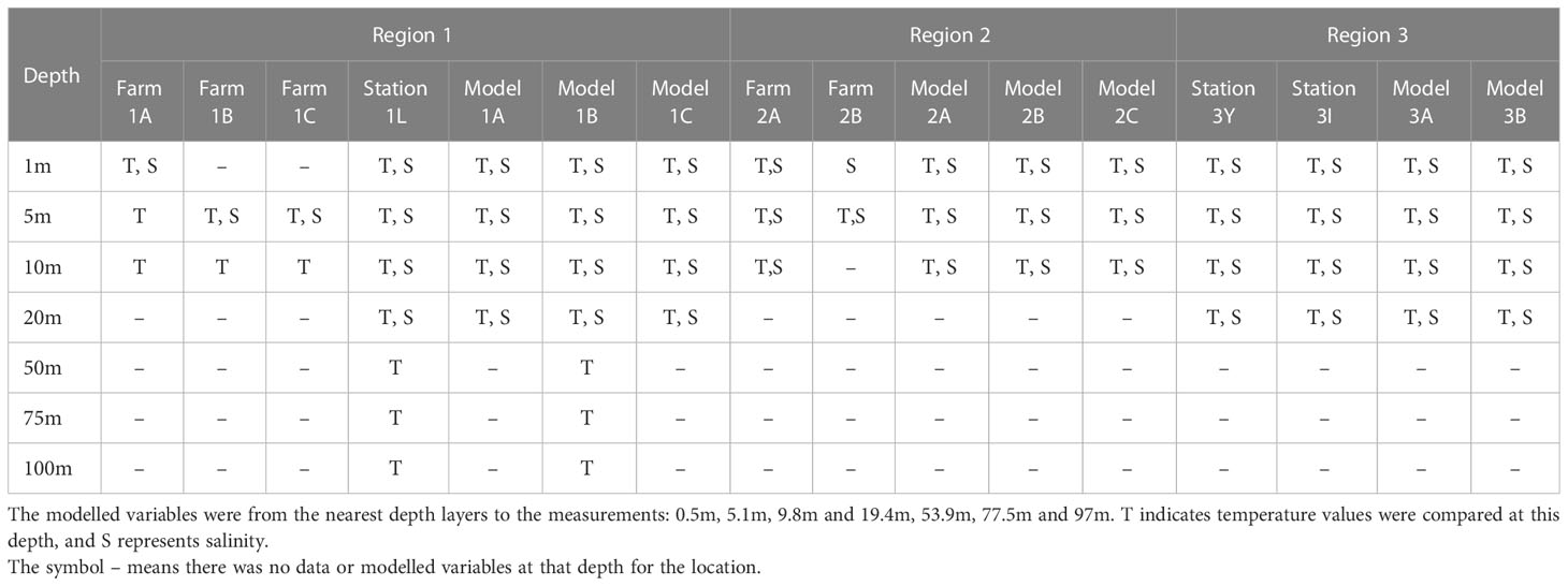
Table 1 The approximate depths used for the comparisons between the measurements from the farms and fixed monitoring stations, and the modelled variables.

3 Results and discussion

3.1 Temperature

Comparisons between modelled and measured temperatures are shown in Figure 2 for Region 1 and Figure 3 for Regions 2 and 3. A similar seasonal cycle in terms of phasing is visible for modelled and measured temperatures, independent of considered depths and sites. The minimum temperatures occur in February/March and the maximum temperatures in August/September. The model and measurements are typically within each other’s standard deviations, however across the sites, months and depths, there are differences in how close the modelled and measured mean values are to each other.

FIGURE 2

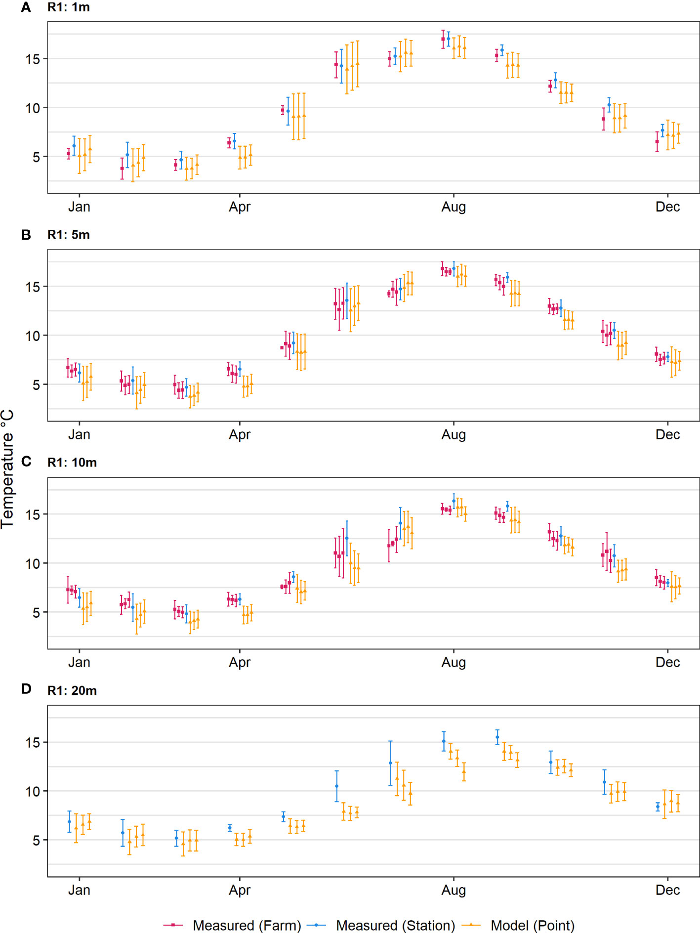
Figure 2 Comparison of modelled temperature versus temperature for the individual farms and stations in Region 1; 5-year monthly average (with standard deviation represented in error bars) for 2016-2020. The rows represent the four depths. The order is as follows: (A) Farm1A, Station1L, Model1A, Model1B and Model1C for 1m depth, (B) Farm1A, Farm1B, Farm1C, Station1L, Model1A, Model1B and Model1C for 5m depth, (C) Farm1A, Farm1B, Farm1C, Station1L, Model1A, Model1B and Model1C for 10m depth, (D) Station1L, Model1A, Model1B and Model1C for 20m depth. Locations are as shown in Figure 1.

FIGURE 3

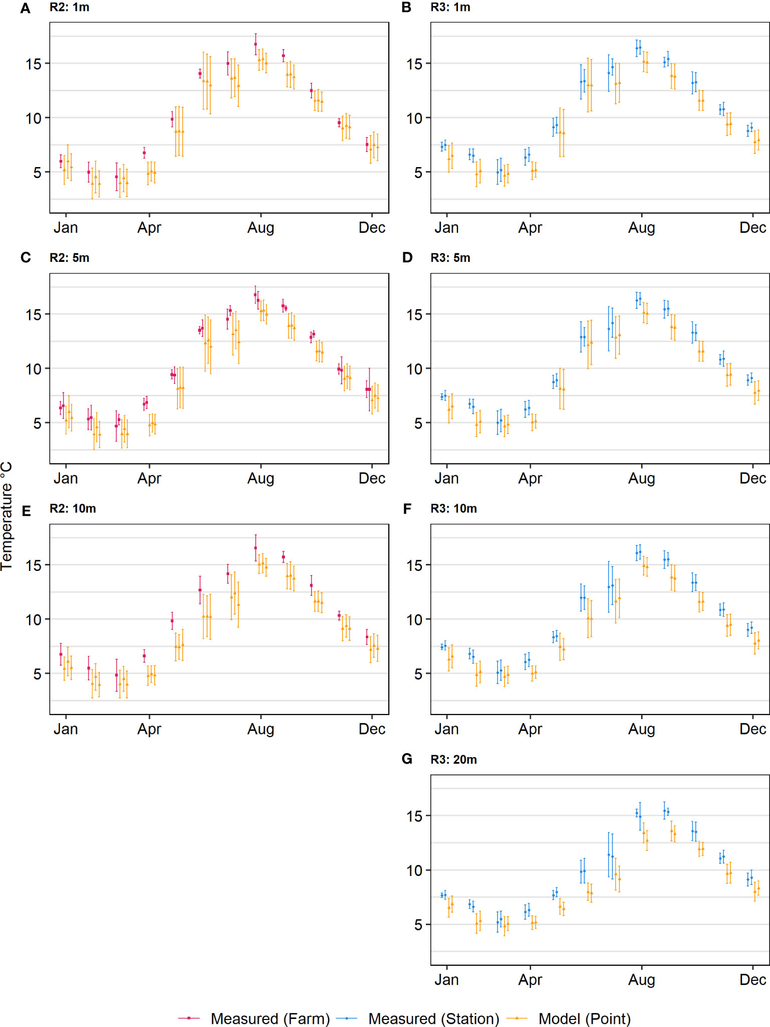
Figure 3 Comparison of modelled temperature versus temperature for the individual farms and stations in Region 2 and Region 3; 5-year monthly average (with standard deviation represented in error bars) for 2016-2020. The columns represent the three regions and the rows represent the four depths. There is no comparison in Region 2 (depth 20m) as farm measurements were not available. The order is as follows: (A) Farm2A, Model2A, Model2B and Model2C for 1m depth, (B) Station3I, Station3Y, Model 3A and Model3B for 1m depth, (C) Farm2A, Farm2B, Model2A, Model2B and Model2C for 5m depth, (D) Station3I, Station3Y, Model 3A and Model3B for 5m depth, (E) Farm2A, Model2A, Model2B and Model2C for 10m depth, (F) Station3I, Station3Y, Model 3A and Model3B for 10m depth, (G) Station3I, Station3Y, Model 3A and Model3B for 20m depth. Locations are as shown in Figure 1.

In Region 1, at 1m depth (Figure 2A) there are months when there are differences between the measured and modelled average values and their standard deviation representing interannual variations. The largest disagreement is visible in April, where the modelled values are 4.9 ± 1.2°C, 4.9 ± 1.1°C, and 5.2 ± 1.0°C in comparison to the farm measurement of 6.4 ± 0.5°C (Farm1A), and the station measurement of 6.6 ± 0.8°C (Station1L). Here, the farm and station measurements agree well with each other despite the station being more offshore, but the model means for all locations in Region 1 are consistently lower than those of the measurements, and the interannual variations are larger within the model. Similar but smaller mismatches can be found in August, September, and October. In some of the other months, the model-means and measurement averages are more comparable. For example, in June the modelled values are 13.9 ± 2.5°C, 14.2 ± 2.4°C, and 14.5 ± 2.3°C in comparison to farm measurement of 14.4 ± 1.3°C, and station measurement of 14.2 ± 1.7°C. Still, the interannual variations in the model appear to be larger than those of the measurements. In autumn and winter, the average values of farm measurements and station measurements diverge, yet the model results for different locations diverge less and vary between being closer to the average station measurement and that of the farm.

At 5m depth (Figure 2B), there are farm measurements available from all three farms in Region 1, and these show similar averages and variations of temperatures in all months as well as a similarity to the measurements of Station1L. The model tends to underestimate the measured temperature values, particularly in April and October. While interannual variability is still higher in the model, the interannual variability of model and measurement are more similar at 5m depth than at 1m depth. At 5m depth (Figure 2B), and at 10m depth (Figure 2C), there are some differences between farms which could be due to the local hydrodynamics (See Figure 1B for farm locations). Likewise, at 10m depth, the station measurements between May and September are visibly higher than the measurements at the farm sites and this could be because the monitoring station is further from the coast. These results show that it is better to use data from multiple farms, and (if available) other sources, to check whether a model is appropriate for a particular area, as temperatures at some farms may be highly localized and not fully representative of other sites. We note that the difference may also be due to limitations associated with measurements (Skogen et al., 2021), as data gaps may have affected the calculation of averages and standard deviations.

In Region 1, the 5-year average modelled temperatures at 10m depth tend to be colder than those measured, which is particularly evident for months April to June (Figure 2C). Differences of several degrees between the modelled and measured average temperatures are also apparent at 20m depth (Figure 2D) in the summer months (June to September). For example, in June the measured temperature at Station1L was 10.5 ± 1.6°C compared to 7.9 ± 0.9°C, 7.7 ± 0.7°C, and 7.8 ± 0.5°C for the model locations. On the other hand, there are also months (January, February, March) when the modelled temperatures are comparable to the station measurements, e.g., in January the measured temperature at Station1L was 6.9 ± 1.1°C, compared to 6.2 ± 1.5°C, 6.6 ± 1.0°C, and 6.9 ± 0.8°C from the model locations. These results suggest that in the examples for Region 1, there were differences in how the model was able to simulate temperatures across the year. Thus, although the model simulated the phasing of the seasonal cycle well, the model underestimated the summer temperatures on average, particularly at 20m depth.

In Region 2, at 1m depth (Figure 3A), average farm measurements are within the standard deviation of that simulated by the model in winter months, while the model underestimates the average temperature for months April to September. In May, the modelled values were 8.7 ± 2.3°C, 8.8 ± 2.3°C, 8.7 ± 2.3°C in comparison to 9.9 ± 0.7°C at the farm. In Region 2, the model simulates larger interannual variations than measured for all months and depths (Figures 3A, C, E). For Region 3, the model results are close to, or are underestimating the average temperature for all depths considered and most months of the year, but are typically within each other’s standard deviations at 1m, 5m and 10m depth (Figures 3B, D, F). Although at 20m depth some months (e.g., May, June, September) showed some differences between modelled and measured values (Figure 3G). These findings show that it is difficult to generalize the differences between modelled projections and measurements, indicating that the usability of a model is dependent on the region, location, depth, and/or time of year.

One question that aquaculture users may have is whether to use projections from individual grid cells or a spatial average, i.e. an average over multiple grid cells for a region of interest. One of the main reasons for choosing a spatial average is that individual cells represent only a small part of the fine-scale dynamic environmental field in the area, thus selecting variables from just one cell may lead to unrepresentative values. This is especially a concern at the coastal interface due to complexities of modelling such areas (e.g., lack of topographic wind effects in fjords and narrow straits due to the use of global atmospheric forcing, coarse topography, or lacking or poorly modelled coastal processes such as river runoff). Figure 4 shows a comparison of modelled and farm temperatures at 5m depth for Region 2, alongside the regional average of the projected temperature for Region 2 (Model2R). Since the station measurements and model locations from Region 3 are still within close proximity to Region 2, they were also included to represent locations further from the coast. The results show that the temperature averages for the individual model grid cells are more similar to each other and the regionally averaged model temperatures than they are to those of the farm and station measurements. In some months (e.g, May, September, October), the simulated temperatures for the individual model grid cells are mostly within the error bars of the regionally averaged model temperatures, suggesting that the modelled conditions are relatively homogenous in that area at those times. For example, in May, the average modelled temperature from the individual model points were 8.1 ± 1.9°C for Model2A, 8.2 ± 1.9°C for Model2B, 8.2 ± 1.9°C for Model2C and the regional average (Model2R) was 8.2 ± 1.8°C. These were also similar to the modelled temperatures for the individual model points in Region 3, which were 8.2 ± 1.9°C for Model3A and 8.1 ± 1.8°C for Model3B. The homogeneity is not seen as clearly in the measurements, as the station measurements further from the coast were colder than the farm measurements in the fjord between April and July. This suggests the model may be unable to correctly reproduce small scale processes in the area at those times. However, in December to March, there is a clear distinction between higher average temperatures for the model locations that are further from the coast (Model 3A, 3B) and at the mouth of the fjord (Model 2B), compared to simulated lower average temperatures in the fjord (Model 2A, 2C). This difference between warmer average temperatures in open waters and colder average fjord temperatures in winter is also seen between farm measurements in Region 2 (which are in the fjord) and the station measurements in Region 3 (which are outside the fjord in more open waters). This suggests a misrepresentation of spatial temperature gradients in summer months for the model. For most of the winter months when there is less homogeneity, the average temperature for Model2R is more similar to Model2B (mouth of the fjord) and Model3A and Model3B (outside the fjord) than Model2A and Model2C (inside the fjord). These findings show that it is useful to compare the regional average and several individual grid cells as part of a model vetting process. In comparison to other aquaculture production regions in Norway (Figure 1A), Region 2 is small and covers an open fjord system. In other regions, there may be greater differences between individual model grid cells and regional averages.

FIGURE 4

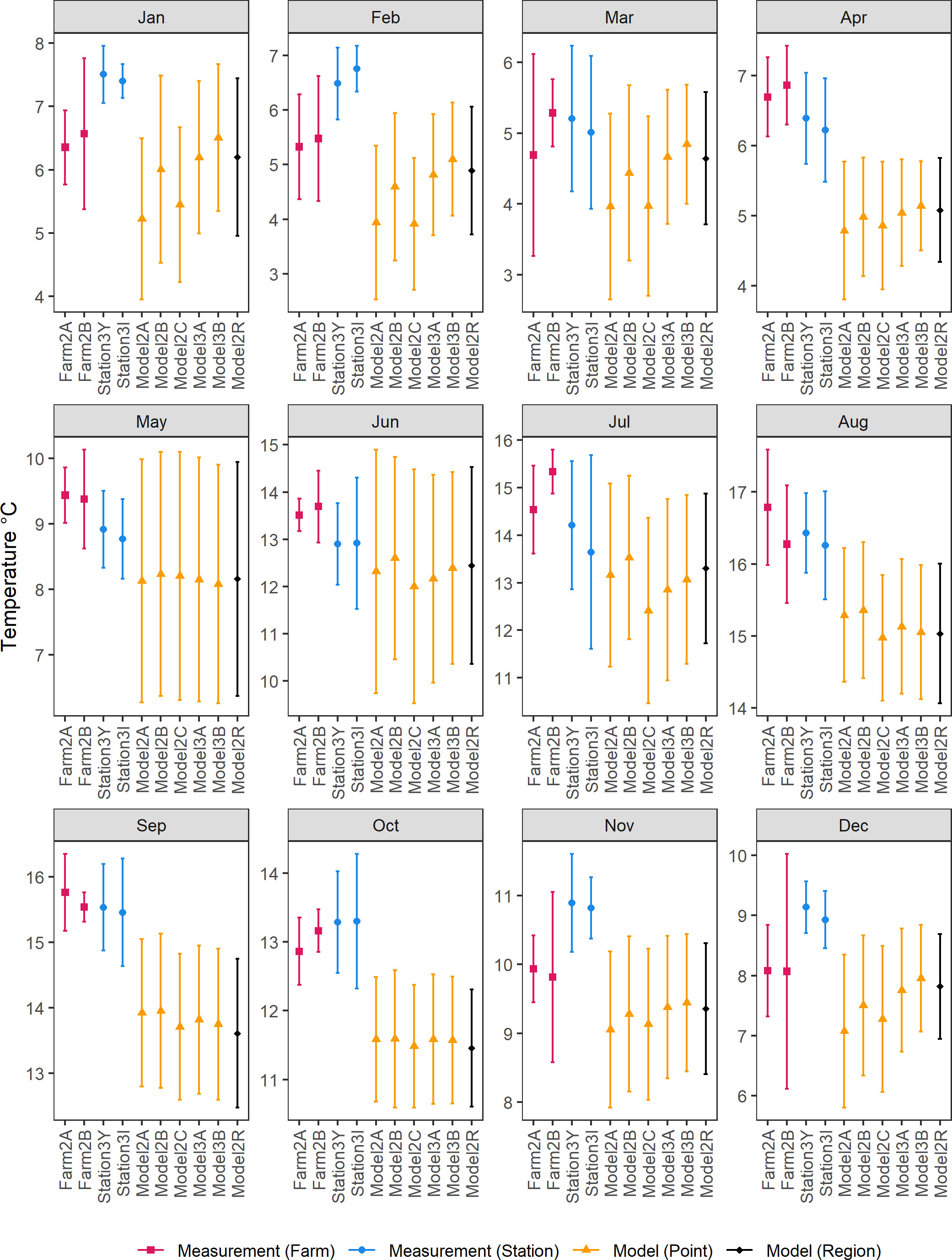
Figure 4 Comparison of modelled temperature versus temperature at 5 meter depth; 5-year monthly average (with standard deviation represented in error bars) for 2016-2020 for Farms in Region 2 (Farm 2A, 2B), Stations in Region 3 (Station 3Y, Station3I), climate model points in Region 2 (Model2A, 2B, 2C) and Region 3 (Model 3A, Model 3B), and the regional average for production region no 2. Locations are as shown in Figure 1.

Depending on the intended use of the climate model projection, it may be appropriate to consider the vertical profile rather than single depths. Figure 5 shows the monthly vertical profile (five-year average with standard deviation) down to 10m depth, of modelled and farm measured temperature for Farm1A and Model1A in Region 1. The model and measurements show similar seasonal values throughout the water column for most months, with both model and measurements indicating a seasonal thermocline. The farm measurements show that there can be differences of several degrees between different depths. For the month of December, the farm measurements were 6.5 ± 1.0°C at 1m depth, 8.1 ± 0.7°C at 5m depth and 8.5 ± 0.8°C at 10m depth, whilst in June the farm measurements were 14.4 ± 1.3°C at 1m depth, 13.2 ± 1.6°C at 5m depth and 11.0 ± 1.5°C at 10m depth. The modelled temperatures for December were relatively similar across the depths, with temperatures of 7.2 ± 1.5°C at 1m depth, 7.3 ± 1.6°C at 5m depth, and 7.6 ± 1.5°C at 10m depth. However, the average modelled temperature for June did show more difference through the water column with 13.9 ± 2.5°C at 1m depth, 12.6 ± 2.2°C at 5m depth, and 10.0 ± 2.1°C at 10m depth. It is important to evaluate how the model simulates conditions at different depths throughout the year since salmon move vertically in the pen due to environmental preferences and behavioral responses (Oppedal et al., 2007), and thus may be positioned at different depths depending on the site, conditions, and time of year. Likewise, stratification influences conditions in the farm (Johansson et al., 2007), and could then influence growth, health, welfare, and overall production in the farm. Therefore, depending on how the aquaculture users intend to use the climate model projections, they may need to consider multiple depth layer(s) from the model and evaluate how the model simulates the site conditions for each depth layer. Most climate models have a refined vertical resolution near the surface, for example the NEMO-NAA10km used in this study has 8 depths available in the upper 10m, but datasets of farm measurements for multiple depths tend to be limited.

FIGURE 5

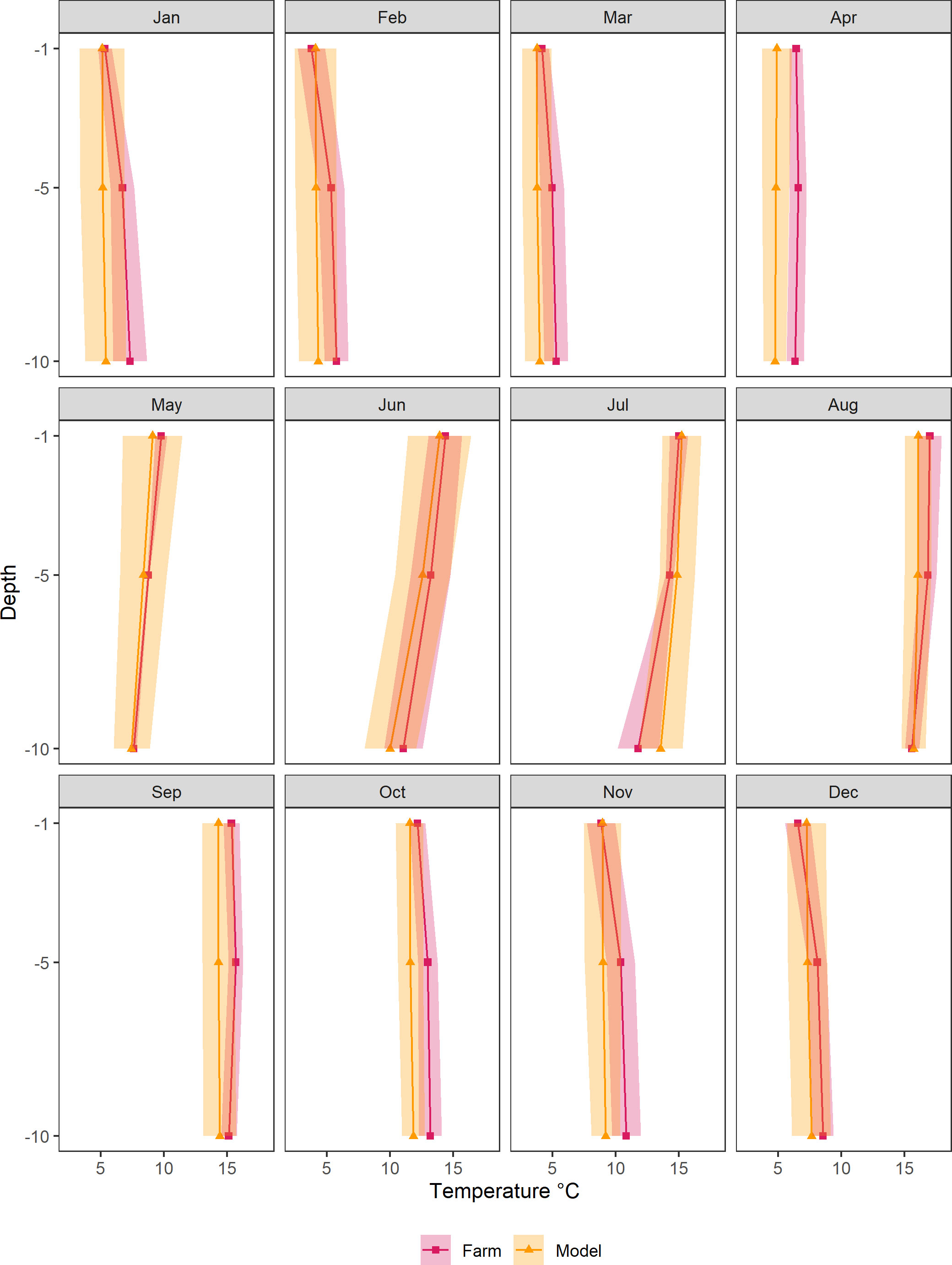
Figure 5 Monthly vertical profile (five-year average is shown with the line and points with standard deviation represented by shaded area) down to 10m depth, of modelled (Model1A) and farm (Farm1A) measured temperature for Region 1.

Furthermore, whilst it is important to consider the conditions within a net-pen farming environment, it may also be desirable to consider future farming systems. For example, there is increasing interest in offshore and submerged aquaculture (Sievers et al., 2022), therefore studies may have to consider conditions at greater depths than those used for traditional net-pens. Farm data was only available to 10m depth, but comparison of the temperature at 100m depth from model with the fixed monitoring station shows clearer seasonal stratification (Figure 6). The average temperature profile of model and measurements are similar in winter months, but there are notable differences in summer months. In summer, the model suggests on average a much steeper thermocline than the station measurements. For example in June, the station measurements were 14.2 ± 2.4°C at 1m depth, 13.6 ± 2.6°C at 5m depth, 12.5 ± 2.6°C at 10m, 10.5 ± 2.1°C at 20m, 7.5 ± 0.6°C at 50m, and 7.3 ± 0.2°C at 100m, and the modelled temperatures were 14.2 ± 2.4°C at 1m depth, 13.0 ± 2.0°C at 5m depth, 9.5 ± 1.8°C at 10m, 7.7 ± 0.7°C at 20m, 7.5 ± 0.5°C at 50m, and 7.4 ± 0.4°C at 100m. Stratification is complicated and depends on site characteristics and hydrodynamics, e.g., whether a site is in the open ocean, along the coastline, or in a fjord (Stigebrandt, 2012; Asplin et al., 2014), and therefore requires site specific context when considering use of climate models. Understanding variable conditions across depth profiles is also important for future development of production technology, as climate projections can also help inform what conditions the farming systems will have to tolerate. To support such assessments there is a need for more high quality, long-term in-situ observations at a range of depths and locations aiding the vetting of considered climate models.

FIGURE 6

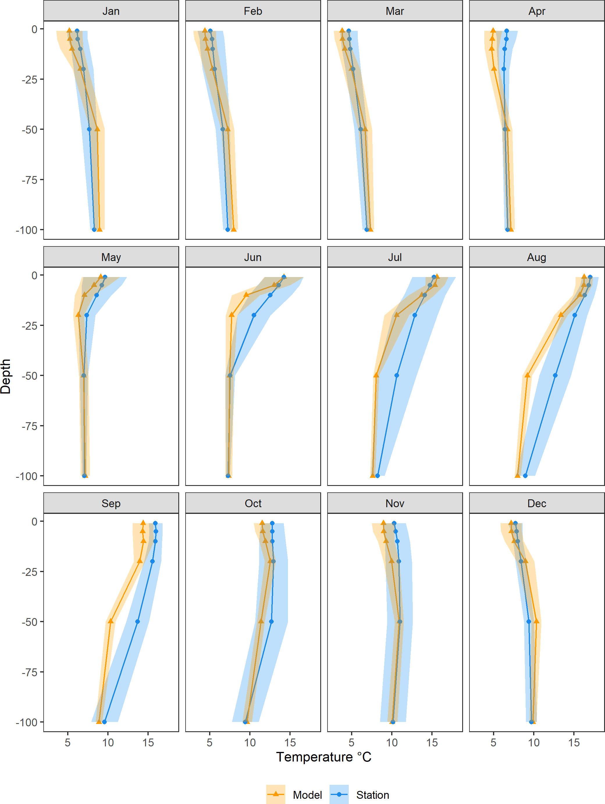
Figure 6 Monthly vertical profile (five-year average is shown with the line and points with standard deviation represented by shaded area) down to 100m depth, of modelled (Model1B) and station (Station1L) measured temperature for Region 1.

3.2 Salinity

Modelled salinity and measured salinity are shown in Figure 7 for Region 1 and Figure 8 for Regions 2 and 3. A seasonal cycle with a summer minimum is seen in the modelled salinity, although the station measurements indicate that the summer minimum of the model is too low in the depths of 1m and 5m. The modelled values are generally similar to the station measurements at 10m and 20m. The results show that there are challenges in using the modeled salinity for near-surface conditions at aquaculture sites that are in coastal areas and fjords.

FIGURE 7

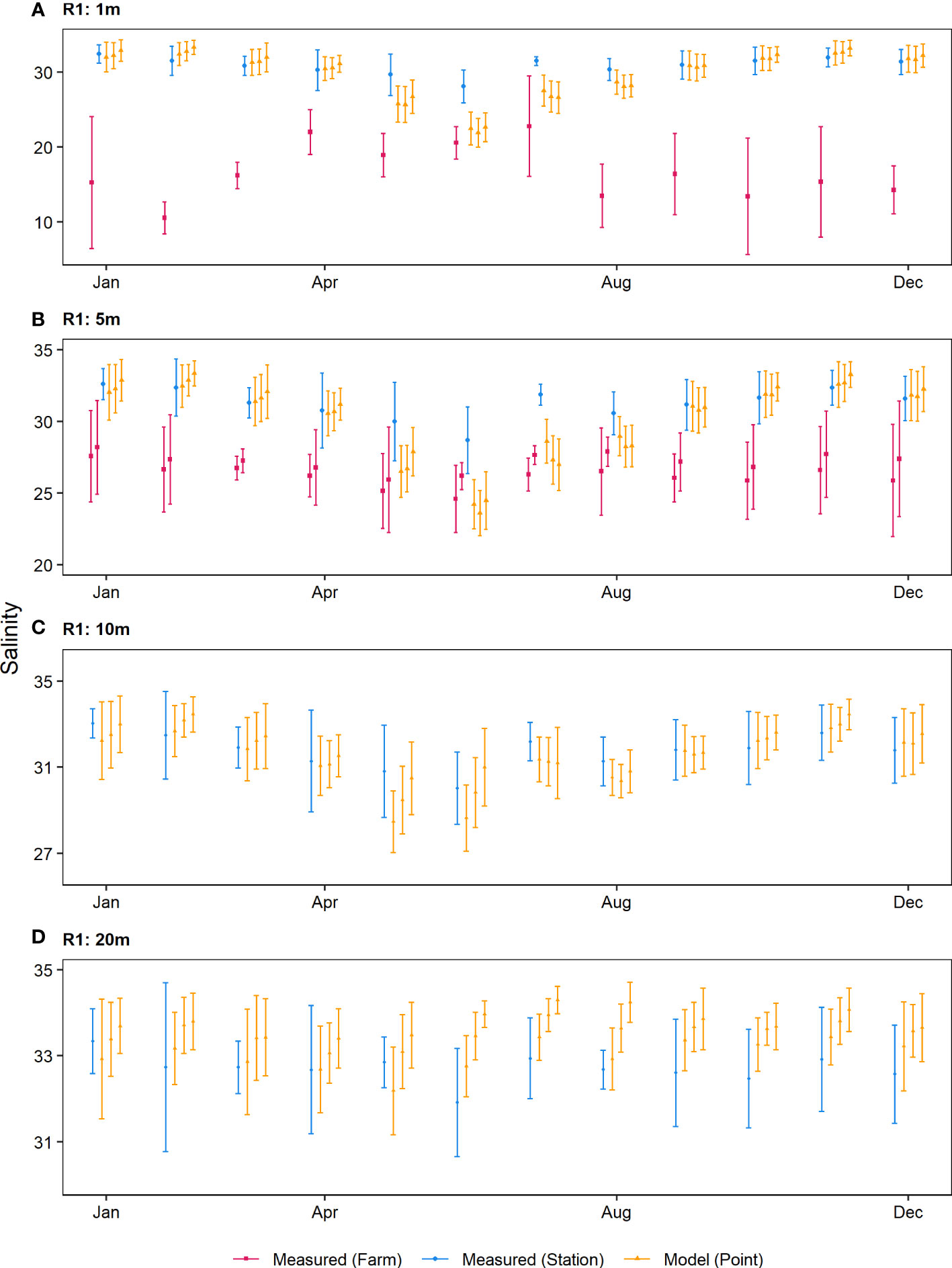
Figure 7 Comparison of modelled salinity versus measured salinity for Region 1; 5-year monthly average (with standard deviation represented in error bars) for 2016-2020. Note that different scales are used. The rows represent the four depths. The order is as follows: (A) Farm1A, Station1L, Model1A, Model1B and Model1C for 1m depth, (B) Farm1B, Farm1C, Station1L, Model1A, Model1B and Model1C for 5m depth, (C) Station1L, Model1A, Model1B and Model1C for 10m depth, (D) Station1L, Model1A, Model1B and Model1C for 20m depth. Locations are as shown in Figure 1.

FIGURE 8

Figure 8 Comparison of modelled salinity versus measured salinity for Region 2 and Region 3; 5-year monthly average (with standard deviation represented in error bars) for 2016-2020. The columns represent the three regions and the rows represent the four depths. Note that different scales are used. There is no comparison in Region 2 (depth 20m) as farm measurements were not available. The order is as follows: (A) Farm2A, Farm2B, Model2A, Model2B and Model2C for 1m depth, (B) Station3I, Station3Y, Model 3A and Model3B for 1m depth, (C) Farm2A, Farm2B, Model2A, Model2B and Model2C for 5m depth, (D) Station3I, Station3Y, Model 3A and Model3B for 5m depth, (E) Farm2A, Model2A, Model2B and Model2C for 10m depth, (F) Station3I, Station3Y, Model 3A and Model3B for 10m depth, (G) Station3I, Station3Y, Model 3A and Model3B for 20m depth. Locations are as shown in Figure 1.

Region 1 at 1m depth shows the largest differences between modelled and measured average salinity values when considering the farm measurements of Farm 1A (Figure 7A). Farm measurements and model show opposing seasonal cycles with average minimum salinity in June (model) in contrast to average minimum salinity in February (farm measurements). In June, the measured salinity was 20.6 ± 2.2 at Farm1A, and the modelled salinity was 22.5 ± 2.2, 21.9 ± 1.9, and 22.6 ± 1.9. In February, the measured salinity was 10.6 ± 2.1 for Farm1A, and the average modelled salinity was 32.4 ± 1.5, 32.8 ± 1.3, and 33.3 ± 0.9. At 5m depth (Figure 7B), measurements from Farm 1B and 1C are available, which show some differences in average salinity to the modelled results, with a general overestimation of salinity in the model and an overestimation of the amplitude for the seasonal cycle, but no signs of a reversed seasonal cycle as seen for Farm 1A for 1m depth. Across all depths, the modelled salinity is more similar to the station measurements. The reason for the differences between the farm measurements and the station measurements is likely due to their locations. The farms in Region 1 are in coastal locations, whereas the station is further from the coast. Compared to the open ocean, coastal areas and fjords have complex salinity profiles as there is a greater likelihood of influence from riverine inputs and runoff (Aksnes et al., 2009; Frigstad et al., 2020). Local-scale river runoff are not considered within the climate model, but freshwater is released at collocated sites along the coast, see Figure 1 for examples from Region 1-3. This simplified modelling approach does not capture all of the runoff points that would influence salinity at local-scale so it is unsurprising that there were differences between modelled and measured salinity.

In Region 2 at 1m and 5m depth (Figures 8A, C), the measured average salinity at the farms shows a weaker seasonal cycle than the model with the model overestimating average salinity for most of the months. At 10m depth (Figure 8D), the modelled and measured average salinity values are comparable for May, July, and September, yet the model overestimates the average salinity for most of the months including March when the measured salinity was 29.8 ± 3.0 for Farm2A and the modelled salinity was 32.9 ± 0.7, 33.4 ± 0.7, and 33.2 ± 0.7.

The differences between the modelled and measured salinity at farm sites are important since salinity is one of the main environmental factors that contributes to some of the most serious health challenges in salmon aquaculture; Ameobic Gill Disease (AGD) (Clark and Nowak, 1999) and sea lice infection (Bricknell et al., 2006; Crosbie et al., 2019). Crosbie et al. (2019) showed that sea lice (Lepeophtheirus salmonis) prefer high seawater salinity and nauplii avoid salinities below 30ppt. Therefore, use of modelled salinity that suggests a site is more brackish than it actually is (or vice versa) could affect disease management and site selection.

There were challenges in obtaining sufficient salinity data for assessments at aquaculture farms as it is not a variable that is routinely recorded at all sites, and fixed monitoring stations are only available in certain locations. Although not focusing on aquaculture, Poste et al. (2021) found that monthly monitoring was insufficient to capture variability and extreme events, and they recommended more frequent monitoring in more locations in the Norwegian land-coast interface to understand how climate change is affecting these areas, particularly regarding the spring snowmelt floods.

3.3 Challenges in comparing modelled projections and observations

Comparisons between climate model projections and measurements must be considered with several caveats. This study focused on a 5-year time period (2016 -2020), as this was the starting period of the climate model simulation and it overlapped with the available observational data. However, these years may be influenced by the climate change scenario used, and thus not fully representative of present-day conditions. As climate projections simulate conditions based on assumptions that may or may not come true, comparisons of this overlapping period are limited to the early years of the projections. Climate models often have a historical run or hindcast that simulates past and present-day conditions and could be compared to long-term datasets from institutional monitoring programs over multiple decades, but historical data is limited for most farms.

It is difficult obtaining sufficient farm-level data of high enough quality that can be used for a comparison with models. Some countries, such as Norway, have long-term monitoring stations in their coastal waters that are extremely useful for studying long-term trends and changing conditions (Albretsen et al., 2012). However, since aquaculture involves holding the farmed species in a fixed position, it is the conditions at that location that are of interest, and this may not be within the vicinity of a monitoring station. Station1L is less than 20km from Farms 1A, 1B, and 1C, but the station is located off the coast in exposed conditions, compared to the farms which are more sheltered and closer to the land. Hence, it is unsurprising that there were differences in measured variables such as salinity. Additionally, in an aquaculture context, the spatial context also refers to the vertical position in the water column. In agreement with Jansen et al. (2016), this study has shown the importance of obtaining farm measurements over multiple depths.

Long-term good quality data collected at individual farms is essential for characterizing conditions and quality checking climate model projections at local-scale, especially in coastal environments. As this study has highlighted, even in areas where aquaculture has long been established, it can be difficult to obtain the type and volume of desired measurement data. Measurements of environmental variables are collected and recorded for a range of different purposes, but there is a lack of standardization and consistency in how data is collected. It is strongly recommended that efforts are made to address data gaps and encourage continuous, high-qualitive in-situ monitoring over long time periods at aquaculture sites, making it possible to characterize conditions and gain insight through measured data in how the farm environments are changing. Data gaps or lack of observational data are not unique to aquaculture and similar challenges have been highlighted in other studies (Jones et al., 2016; Dorigo et al., 2017; Mottram et al., 2021). In addition, measurements do not necessarily represent true conditions as there can be representativity issues as well as inconsistencies and errors during data collection and analysis (Sampaio et al, 2021; Skogen et al., 2021), and it is important to also consider the context of how measurements are used in any model evaluation process. Many aquaculture datasets have relied on manual data collection and recording, with data availability and quality affected by many factors, including challenging weather conditions, monitoring equipment, lack of common protocols, and differences in how people collect and store the data. Increasing use of automated sensors and digitalization of the sector offers opportunities for the collection of more in-situ measured data (O’Donncha and Grant, 2019), and there would be benefits from industry-wide cooperation to standardize how data is collected and stored.

In comparing models and observations, it is important to be realistic. Whilst well-performing climate models may provide a decent large-scale description of the environment, perfect match in space and time between low-resolution model output and site-specific measurements should not be expected. Model evaluation depends on the intended use of the climate projection and it is not possible to apply simple rules or thresholds to infer good or bad fit (Knutti, 2018). Of course, there are many different approaches and statistical tests that can be used to evaluate climate model projections (Baumberger et al., 2017; Knutti, 2018), and some may be more appropriate than others under given circumstances. A more robust approach may be to use a combination of evaluation methods, including knowledge from those familiar with the model, area, and the precision required in any subsequent analysis. There is no single definitive way of establishing if a model is acceptable for use for aquaculture generally or at a specific site, especially as there will be many different potential applications, e.g., investigating species growth potential, risk of mortalities, possible spread of disease, or location of future farms, all of which require different levels of information and precision. Acceptance of a model will depend on the user’s own judgements (Bennett et al., 2013), and that requires appreciation of contextual factors behind the modelled and measured values, as well as the farm characteristics and intended use of the information.

It is not the intent of this paper to direct users of climate models to a certain method or approach, but rather to raise awareness that models, measurements, and purpose must be thoroughly considered. The present study used one scenario and one climate model, and it is highly likely that other climate models, or (multi)model ensembles, would have different results due to model uncertainty, separated into structural uncertainty (inability to understand and/or describe a process) and parametric uncertainty (many small-scale processes need to be empirically described rather than resolved due to lack of knowledge) (Knutti et al., 2010). Furthermore, this study focused on a monthly comparison due to availability of data and visualization purposes, but it is important to acknowledge that many aspects of the health, welfare and behavior of aquatic species are influenced by the temperature of their surrounding environment at a much shorter time scale. Hence, for aquaculture purposes, and for variables like temperature, time averages can mask conditions that challenge the fish (Sampaio et al., 2021).

3.4 Model vetting framework

The term vetting is used here to refer to the process by which aquaculture users can determine whether they can use climate model outputs for their specific purpose. Users should be mindful that a comparison of historical or present-day conditions provides context for the model but does not necessarily mean that the model will perform well for the future scenario. A simple vetting framework is outlined in Figure 9. There are several stages, and as model vetting progresses there may be a need to revisit earlier steps and try alternatives. At each stage of the vetting process, communication between aquaculture users (e.g. researchers, aquaculture producers, other industry stakeholders) and climate modelers would enhance understanding and clarify misunderstandings. We are using the term aquaculture users to cover a wide range of groups as there are many different people within the aquaculture sector who could make use of climate projections in addition to researchers. For example, timeseries of future temperatures could be used by aquaculture producers to assess risks to existing and future sites, but they could also be used by feed manufacturers to help identify future feed strategies, or by veterinary pharmaceutical companies to evaluate long-term efficacy of existing treatments. Furthermore, although this study used examples from Norwegian salmon farms as illustrations of some of the considerations, the findings are relevant to other types of marine aquaculture and the vetting framework can be used for other species and farms.

FIGURE 9

Figure 9 Overview of the climate model vetting framework for aquaculture users.

3.4.1 Establish the context

Aquaculture users must decide what they intend to use the climate model for. This will determine the information they require and help establish what contextual information will be required. Aquaculture site characteristics vary considerably between farms so there is a need to understand the area under investigation and identify potential factors that may be difficult for models to incorporate, e.g. unpredictable freshwater inputs or other external influences. Likewise, climate change could affect many different aspects of aquaculture (Falconer et al., 2022), and it is important to establish what the climate model outputs would be used for. At this stage, aquaculture users and climate modellers should start discussions on what is desired and what is possible. Aquaculture users should provide information on the site(s) they are interested in using climate information for. As this study has highlighted, relevant characteristics would include whether the site is in a fjord or open ocean, is in a shallow or deep location, and if there are nearby river or runoff points. Any contextual information about the site, and factors that may influence the variables of interest should be highlighted by the aquaculture users. The climate modellers should explain what climate models are available for the specific location and what projections or simulations can be provided.

In this study, we used temperature and salinity projections from a regional model downscaling, but aquaculture users will have to identify what model projections are available for their area of interest. There are many climate models available, for example, the sixth and latest phase of the coupled model intercomparison project (CMIP6) (Eyring et al., 2016) includes 312 experiments (Petrie et al., 2021) and anticipated output-data from at least 100 models hosted by 40 modelling centers (Balaji et al., 2018), though not every model participated in every experiment. Additionally, several regional ocean models have run one or more climate change scenarios from the CMIP6-framework without providing their output to the CMIP6-database. There are different routes to which the aquaculture community can access climate model information, either through the CMIP6 database or through personal communication with a climate modelling center. It is important that aquaculture users have an appreciation of some of the key aspects of the model, such as the model resolution, if and how the variable of interest is calculated, and how well the chosen model can represent the variable of interest. This serves as a starting point as aquaculture users will have to decide whether they use e.g. a global model or a higher-resolution regional downscaling (if available).

Depending on the experience level of the aquaculture user, the climate modeller may have to provide some background information and context about climate models and scenarios to assist discussions on choice of models. In this study we used climate projections from one SSP scenario, SSP2-4.5 as an example, but when investigating the future, aquaculture users will usually want a range of potential future scenarios.

Climate models often have a hindcast simulation forced by an observed atmospheric forcing (reanalysis) that results in a variability in oceanic variables that is comparable to observed timeseries. However, though hindcasts often go back decades, it is rare to have farm records of climate parameters over such a long period. On the other hand, the CMIP6 SSP scenarios start in the year 2015, so there is a relatively recent time period available for comparison with measurements, as used in this study. We note that climate projections of SSP scenarios are usually built upon a historical simulation such that it is also possible to use, for example, years 2000-2014 from the historical simulation and years 2015-2020 from the considered SSP scenario.

3.4.2 Define goals and select criteria

With an understanding of the aquaculture site(s) and information requirements, as well as the model capabilities, the aquaculture user can define goals and select desired climate model criteria. This includes selecting the variable(s), areas, times and depths of interest. Available variables will depend on the model(s), and some are more commonly simulated than others, e.g. temperature is always available. At this stage, aquaculture users should work with climate modellers to identify what is available, and how it could be used. Since many of these choices depend on the intended use of the climate projections and what can be provided by the model, there may be trade-offs involved that could lead to a need to revisit the scope of the application.

3.4.3 Comparison between model outputs and in-situ measurements

The present study has highlighted the importance, and challenges, of comparing model outputs with in-situ measurements. The results of the comparisons showed that it is difficult to generalize differences across time of year, depths, variables, and locations within and between regions. Consequently, where possible, each variable, area, time, and depth that is intended for use should be evaluated, as model outputs may be appropriate for one but not another location and variable. Aquaculture users can also work with climate modellers to do the comparison, and then interpret and discuss the findings.

This study is not suggesting a strict protocol for comparisons as it will be highly dependent on the availability and quality of in-situ data and will also depend on the intended use of the climate projections. However, there are several considerations that aquaculture users must think about. First, the aquaculture user must identify what data is available. Since long time-series are required for comparison, in many cases the aquaculture user will be reliant on existing datasets as generation of new data would take too long. Farms routinely measure variables such as temperature, although data may not be stored or archived for long-term use. There can be inconsistencies in data collection and storage, and there are usually gaps in recorded variables when the farm is not stocked, which introduces complications. In the case of uncertainties with datasets it is advisable to use multiple independent data sources, as done in this study with the station and farm measurements. The results of this study have shown that it is also important to consider which form of model output to use in the model-observation comparison, in order to find a representative climate projection for the site in question. In a comparison it is advisable to use simulations from multiple individual grid cells within the proximity of the farm site(s), and if relevant, a spatial average may be included as well.

A range of approaches are available to compare models and measurements, and these have been discussed by others (e.g. Stow et al., 2009; Bennett et al., 2013). Choice of approach will depend on several factors, including data availability, data quality and how the comparison will be interpreted. This study used comparisons of 5-year monthly averages (and standard deviations), but monthly averages could miss conditions relevant to aquaculture production (Sampaio et al., 2021). Decisions on temporal resolution will be constrained by what data is available, but it is important not to forget the overall goal. Therefore, aquaculture users should discuss their expectations with climate modellers, who can use this information to help identify appropriate approaches to assess model skill. At this point, aquaculture users should also highlight potential time-critical factors (e.g. if they are using the model to simulate changes in stocking date).

Statistical tests for comparisons may also be limited by a lack of, and/or inconsistent monitoring of, environmental data. In the present study, a visual comparison was used. Whilst this may seem like a simple approach, in many cases visual evaluation and consultation with industry experts familiar with the area is useful in model vetting and can provide a platform for aquaculture users and climate modellers to discuss if and how climate models can be used for the intended goal. In other situations, studies have shown that local knowledge can provide important context for climate information (Clifford et al., 2020; Streefkerk et al., 2022). Accordingly, even if statistical tests are used for comparisons, then there is still value in providing a visual representation as well.

3.4.4 Decision

The model vetting framework provides a structured and objective approach to understanding the context in model use and application within aquaculture. However, model vetting will still involve some subjective judgements of how generated results would be used to make decisions and whether this is appropriate. Consequently, the final step is for aquaculture users to decide whether the model output is appropriate for their intended use. This could mean using the model output directly, or calibrated in some way, e.g. as highlighted in Falconer et al. (2020). However, as illustrated in the surface salinity example in Region 1, it is important to recognize that there may be cases when models cannot be used for a particular purpose, or the aims need refinement. Climate models are not intended to simulate the exact atmospheric/oceanic conditions that were measured at a certain time, but rather a mean climactic state of a certain period, and so there will be some aquaculture questions that are outwith the scope of model possibilities. Discussions with climate modellers can help aquaculture users come to a decision on the use of climate models.

3.5 Wider implications

Quantifying differences in modelled variables compared to farm-level measurements is useful for aquaculture, as it may reveal important implications for how climate models can be used. Other studies have considered approaches to calibrate global and regional-scale models to farm-level (Falconer et al., 2020; Fuentes-Santos et al., 2021; Stavrakidis-Zachou et al., 2021), but aquaculture users also need to consider the way in which they are interpreting the climate projections. For example, thresholds are a common way of translating climate model projections into potential impact. If modelled values are above or below a threshold value, then they are categorized as a risk or opportunity for a particular aspect of aquaculture. Yet, this interpretation is only rational for a specific farm if the considered model has been shown to simulate the considered variable at the farm level dynamically well.

Climate information is generally underutilized by practitioners and policymakers (Lemos et al., 2012; Kirchhoff et al., 2013), but as shown in the present study, interpretation of climate projections for aquaculture can be supported and improved by model vetting, assuming model skill in simulating present-day climate conditions are related to confidence in future projections. If such approaches are included in impact assessments, this will increase transparency by providing a clearer understanding of how accurate the climate model projections may predict the future aquaculture environment. It is then up to users to make their own judgements on the usability of the information for their particular context. Furthermore, there are clearly many potential applications of climate information in the aquaculture sector, but, as in all sectors, lack of knowledge over the needs of potential users and misguided expectations can be a barrier to effective use of climate information in decision-making (Dilling and Lemos, 2011). To increase usability of climate information and model projections, Lemos et al. (2012) recommend taking steps to improve communication and co-operation between the producers and users of climate information. The presented results support this statement, as collaborative research initiatives between climate modelers, researchers, industry, and policymakers would increase understanding across all parties, improve confidence in the results generated, and hopefully encourage more real-world applications of climate information within the aquaculture sector.

4 Conclusions

The present study demonstrates why it is important for aquaculture researchers, practitioners, and stakeholders to consider how they are using climate information. The results from the Norwegian farm sites and monitoring stations revealed that a model may perform well under one set of conditions, but not at another (e.g. differences between locations, depths, time of year, and variables). For temperature, in some highlighted cases there were differences of 3 degrees between the 5-year averages of measured and modelled values. Whilst some differences between modelled and measured values are expected, drawing conclusions from modelled temperatures 3 degrees lower than they should be would potentially be misleading for many aspects of fish physiology. The results also showed that modelled salinity at some sites was considerably different to measured salinity as the model did not capture the localized river inputs, thus the model 5-year averages were above 30 (seawater), whilst the measured 5-year averages were below 20 (brackish conditions). However, in other cases, for both temperature and salinity, there were very similar modelled and measured values. Therefore, the key recommendation is that aquaculture users need to carefully consider how they are using climate model information and check whether the application is appropriate for their site or if any further processing is needed, for example, bias-correction of temperature. To support this recommendation, we developed a vetting framework that provides a more structured approach for aquaculture users and climate modellers to work together to improve use of climate models in aquaculture.

In many cases decisions on whether climate models are appropriate for use will still involve some subjective judgements and considerations of how the generated results would be used to make decision. There are difficulties in obtaining long-term datasets of in-situ measurements of sufficient quality to allow robust comparisons, and efforts to improve data collection should be encouraged. Furthermore, there are challenges associated with facilitating model output at local scale and assessing the model skill under present day local conditions. However, even if a comparison is limited or equipped with many caveats, it can provide valuable information to support decisions on model use and interpretation of results. Vetting model results to real-world context offers a more transparent approach than blindly using climate models without any vetting.

Data availability statement

The data analyzed in this study is subject to the following licenses/restrictions: The IMR fixed monitoring station data can be downloaded from http://www.imr.no/forskning/forskningsdata/stasjoner/index.html. There are restrictions on the availability of farm data due to confidentiality agreements. The subset of the downscaled climate projections used in this study are available on request to LF. Requests to access these datasets should be directed to Lynne Falconer, lynne.falconer1@stir.ac.uk.

Author contributions

LF, EY and SH: conceptualization. LF: analysis and original draft. All authors contributed to the article and approved the submitted version.

Funding

This work was supported by a UKRI Future Leaders Fellowship (MR/V021613/1) and the Norwegian Research Council No. 194050 (Insight). It was also supported by the Bjerknes Centre for Climate Research through the project SKD-LOES and by the Bjerknes Climate Prediction Unit (BCPU) in Bergen through the Trond Mohn Foundation (Project number: BFS2018TMT01). SL and NG acknowledge funding from the European Union’s Horizon 2020 research and innovation programme under the project ASTRAL (grant agreement No 863034).

Acknowledgments

The climate simulations for this article were made on the supercomputer Fram, which is part of the Norwegian Infrastructure for Research and Education (Sigma2). We thank Dr. Robinson Hordoir, Institute of Marine Research for performing the downscaled climate simulations. We also thank the Norwegian salmon aquaculture producer companies that provided the farm data.

Conflict of interest

The authors declare that the research was conducted in the absence of any commercial or financial relationships that could be construed as a potential conflict of interest.

Publisher’s note

All claims expressed in this article are solely those of the authors and do not necessarily represent those of their affiliated organizations, or those of the publisher, the editors and the reviewers. Any product that may be evaluated in this article, or claim that may be made by its manufacturer, is not guaranteed or endorsed by the publisher.

References

Ådlandsvik B. (2015). Forslag til produksjonsområder i norsk lakse-og ørretoppdrett (Bergen, Norway: Institute of Marine Research), 59pp.

Google Scholar

Aksnes D. L., Dupont N., Staby A., Fiksen Ø., Kaartvedt S., Aure J. (2009). Coastal water darkening and implications for mesopelagic regime shifts in Norwegian fjords. Mar. Ecol. Prog. Ser. 387, 39–49. doi: 10.3354/meps08120