 Graham D. Quartly
 Jim Aiken
 Robert J. W. Brewin
 Andrew Yool
- 1Plymouth Marine Laboratory, Plymouth, United Kingdom
- 2Centre for Geography and Environmental Science, University of Exeter, Penryn, United Kingdom
- 3Marine Systems Modelling, National Oceanography Centre, Southampton, United Kingdom
Satellite observations have given us a clear idea of the changes in chlorophyll in the surface ocean on both a seasonal and interannual basis, but repeated observations at depth are much rarer. The permanently-stratified subtropical gyres in the Atlantic are highly oligotrophic, with most production centred on a deep chlorophyll maximum (DCM) just above the nitracline. This study explores the variations in this feature in the core of both gyres, considering both seasonal and interannual variations, and the linkages between changes at the surface and sub-surface. The in situ observations come from the Atlantic Meridional Transect (AMT), a long-running UK monitoring programme, and also from biogeochemical Argo floats. AMT provides measurements spanning more than 25 years directed through the centres of these gyres, but samples only 2 to 4 months per year and thus cannot resolve the seasonal variations, whereas the profiling floats give coverage throughout the year, but without the rigid spatial repeatability. These observational records are contrasted with representation of the centres of the gyres in two different biogeochemical models: MEDUSA and ERSEM, thus fulfilling one of AMT’s stated aims: the assessment of biogeochemical models. Whilst the four datasets show broadly the same seasonal patterns and that the DCM shallows when surface chlorophyll increases, the depth and peak concentration of the DCM differ among datasets. For most of the datasets the column-integrated chlorophyll for both gyres is around 19 mg m-2 (with the AMT fluorescence-derived values being much lower); however the MEDUSA model has a disparity between the northern and southern gyres that is not understood. Although the seasonal increase in surface chlorophyll is tied to a commensurate decrease in concentration at depth, on an interannual basis years with enhanced surface levels of chlorophyll correspond to increases at depth. Satellite-derived observations of surface chlorophyll concentration act as a good predictor of interannual changes in DCM depth for both gyres during their autumn season, but provide less skill in spring.
1 Introduction
The patterns of ocean productivity are set by physical processes and chemical resources. The Earth’s orbit around the sun and thus the changing solar zenith angle produces an annual cycle in the main forcing terms: solar irradiance (SI) incorporating both photosynthetically available radiation (PAR) and the infra-red components that raise sea surface temperature (SST), increase stratification and, as shown by Levitus (1982), lead to a shallowing of the mixed layer depth (MLD). There is, of course, a daily cycle of heating and night-time cooling, with the latter creating convectional mixing at the top of the water column that disperses those plankton that exist there throughout a seasonal mixed layer. Whilst coastal and well-mixed high-latitude seas have a plentiful nutrient supply, large regions in the tropics are permanently stratified leading to nutrient depletion in the surface waters. This unique environment, controlled by both growth and loss (grazing) processes, leads to low surface concentrations of phytoplankton, with a vertical profile marked by a deep chlorophyll-a maximum (DCM). In this region light levels are very low (typically of order ~1% of that at the surface), but there is sufficient supply of the essential nutrients from a reservoir below. Since growth rates of phytoplankton are fast (doubling time of the order of 1 day), these population profiles must usually be considered as in a quasi-steady state, balancing predation and other loss terms against individuals’ reproduction, noting that the conditions of light and nutrients at the DCM are able to support a larger standing stock of phytoplankton.
Within the Atlantic there are two main oligotrophic regions corresponding to the centres of the northern subtropical gyre (NSTG) and the southern subtropical gyre (SSTG). Each of these gyres occupies about 5% of the Earth’s surface (Aiken et al., 2017), and although low in surface chlorophyll-a they are an important area for research as they may contribute significantly to carbon drawdown. Furthermore, several climate change predictions suggest greater stratification for larger areas of the Earth’s subtropical ocean, so those ecological implications need to be assessed. This study examines the seasonal and interannual variations in the DCM within these gyres, taking particular advantage of the Atlantic Meridional Transect (AMT) programme, which has provided in situ measurements spanning more than two decades. Our goal is in line with a core aim of AMT to provide essential data for global ecosystem model development and validations (Rees et al., 2015). As the timing of these cruises has been tied to the resupply of the UK’s Antarctic bases e.g. Rothera, the cruises have mainly been in September/October to November and in April to May/June (see Figure 1). As the dynamics of the NSTG and SSTG may be somewhat different, we keep the analyses for these two regions separate and are thus considering four seasonal “modes”:
● Boreal spring (northward leg through NSTG) when PAR and SST are increasing
● Austral autumn (northward leg through SSTG) when PAR and SST are declining
● Boreal autumn (southward leg through NSTG) when PAR and SST are declining
● Austral spring (southward leg through SSTG) when PAR and SST are increasing
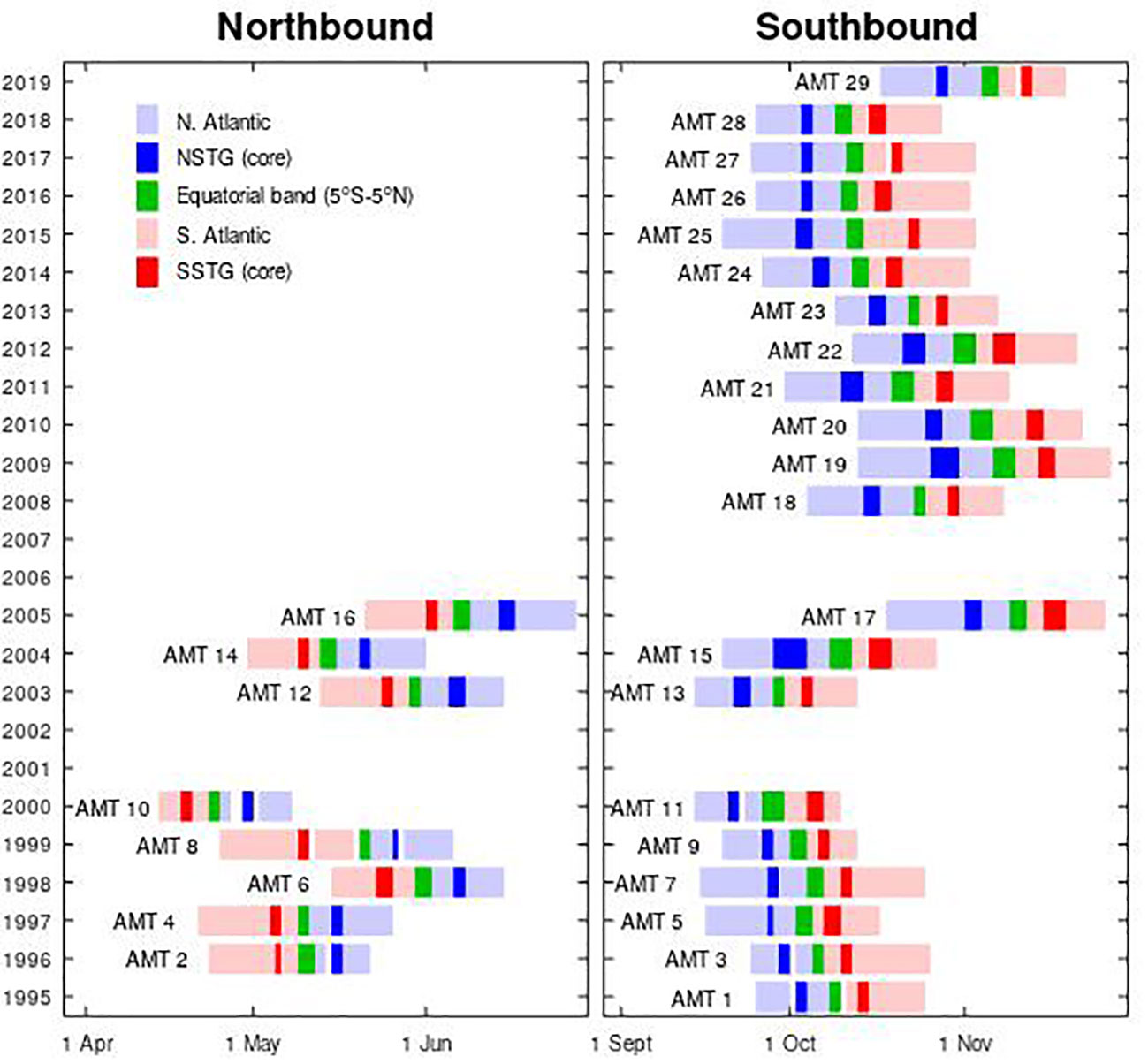
Figure 1 Timelines of the AMT cruises, showing that up to 2006 there were equal numbers in each half of the year, but since then cruises 18-29 have all been southbound (boreal autumn; austral spring). [Image based on Figure 2 of Aiken et al. (2017)].
These analyses are augmented by profiles from biogeochemical (BGC) Argo floats, which do not provide spatially homogeneous coverage, but allow us to look more clearly at seasonal variations. Additionally we look at output from two numerical biological models to assess how well they replicate the seasonal changes in the DCM, and whether they can give us insight into the causal connections between changes in surface and sub-surface properties.
The aim of this paper is to look at the connectivity between surface manifestations of chlorophyll and the developments at the deep chlorophyll maximum, using both in situ and model data. Surface chlorophyll affects distribution below, as it modifies the light penetration at depth. There are clear seasonal variations, because of the annual cycles in forcing, but the challenge is whether sub-surface interannual variations can be inferred from observing the surface only.
2 Data
In this paper, we focus on the use of chlorophyll as an indicator of phytoplankton biomass. This follows standard biological oceanography practice, as it is an easily recorded consistent measure with global standards (see Table 1 of Sathyendranath et al., 2023) and is also one of the currencies used by most biological models, including the two that we had access to for this paper. However, a number of factors do affect the reliability of this measure of plankton biomass along the vertical dimension, including changes in plankton community structure and photoacclimation, viz. phytoplankton’s change in Chl-a content per cell in response to light saturation/starvation (Cullen, 1982; Kitchen and Zaneveld, 1990).
This paper makes use of two sources of in situ data, and output from two different biogeochemical models, plus satellite observations to give the wider context. Note that the in situ measurements detailed in these first two sub-sections are strictly measurements of chlorophyll-a (hereafter denoted Chl-a), both monovinyl and divinyl forms, as they respond to the fluorescence associated with those specific molecules, whereas the fields in the models refer to total chlorophyll (i.e. model fields do not differentiate between the different types of chlorophyll pigment). High Performance Liquid Chromatography (HPLC) for these core regions within the Atlantic gyres indicates that the concentration of Chl-a exceeds that of other chlorophyll molecules (e.g. Chl-b and Chl-c) by almost a factor of ten (Aiken et al., 2017). Furthermore these HPLC measurements showed good agreement with satellite (SeaWiFS) data, suggesting it is reasonable to intercompare these subtly different measurements.
2.1 Cruise data from the Atlantic Meridional Transect programme
The AMT programme provides long-term monitoring of changes in the whole of the Atlantic Ocean by surveying physical and biological properties in the Atlantic Ocean on a roughly yearly basis. The AMT programme has been operational since 1995, and makes use of the need for an Antarctic supply vessel to travel from the UK to the research bases, for example, at Rothera on the Antarctic Peninsula. This endeavour is unique in its scope of sampling a wide range of Longhurst provinces ranging from productive coastal waters to the centre of the oligotrophic gyres. Much of the section is along the 25˚W meridian, but there are variations from year to year according to other scientific or logistical needs. In particular, the route used in the 1990s stayed close to Africa in the northern hemisphere, but was adapted to sample better the NSTG from 2003 onwards (see Figure 1 of Rees et al., 2017).
Each cruise incorporates many CTD (conductivity-temperature-depth) stations, where along with those three essential measurements of physical properties, there are other chemical or biological profiles taken using fluorometers, light sensors and assays of chemical constituents. Here we make use of the estimated chlorophyll-a concentration obtained by a fluorometer attached to the CTD frame. Although efforts are made to calibrate the fluorometer for each cruise, it was noted that in some cases the value at depth was distinctly different from zero. In this paper our focus is on the permanently-stratified oligotrophic gyres, where interannual changes may be small. Data from a number of the earlier cruises are omitted due to concerns about the calibration of the fluorometers. For the remaining ones the average over 250-300 m is calculated and removed from all other measurements, assuming it to be a fluorometer measure of detritus or dissolved substances and/or a calibration error.
The majority of cruises have been on the southbound route to Antarctica during the period September to November; these cruises measured the NSTG during boreal autumn and the SSTG during austral spring. However, in the first phase, several cruises were done on the return leg heading northbound to the UK in April to May, thus sampling the SSTG in austral autumn and the NSTG in boreal spring. A clear depiction of the periods sampled is shown in Figure 1). In our analysis, these two sets of cruises are kept separate, so that we assess the variations in Chl-a profile in the oligotrophic gyres through four different modes: NSTG in boreal spring and autumn, and SSTG in austral spring and autumn. Although one might expect some similarities in behaviour for the northern and southern hemispheres, the currents bounding them do differ e.g. the NSTG will contain some waters from the deep Mediterranean outflow, whilst the SSTG is traversed by Agulhas Rings carrying Indian Ocean water (Nencioli et al., 2018). There are also hemispheric differences in the availability of dissolved organic nitrogen (Clark et al., 2022). Smyth et al. (2017) also illustrate the differences in seasonal forcing for these two gyres. The AMT observations thus allow us some insight into annual variations albeit from just two seasons of the year.
2.2 BGC-Argo profiling floats
Argo profiling floats have been providing temperature and salinity data in the world ocean for approximately 20 years (Wong et al., 2020), with the target of 3000 floats sampling every 10 days reached in 2007. Biogeochemical (BGC) sensors have been added to a small but growing number of floats, but their deployment and operation has been driven more by individual research projects, rather than the aim of establishing quasi-global coverage. Therefore there may be a series of floats in one region with frequent (daily or sub-daily) sampling, whilst others regions have had few floats. We use here the data-field termed “CHLA_ADJUSTED” as Roesler et al. (2017) have pointed out that the data from the factory calibration typically lead to an overestimate of the amount of chlorophyll by a factor of two on average. We also make some correction (see below) using the estimated Chl-a values at depth. In the present work we have considered measurements representative of the SSTG if they are within 5˚ longitude and 5˚ latitude of 25˚W, 20˚S and have a surface chlorophyll value less than 0.1 mg m-3, with a similar-sized box around 38˚W, 24˚N for the NSTG. There are profiles in these regions for all years since 2012 (see Figure 2), but not always in all seasons.
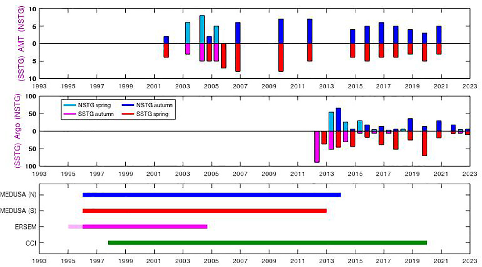
Figure 2 Time span of the various datasets. The AMT cruises occur in Apr-May or Sept-Nov, with a tendency in the last 15 years for observations in the latter period as the ship heads southbound to supply the Antarctic bases. However, not all cruises make measurements in the NSTG or SSTG, depending on their route. The BGC-Argo data are very heterogeneous, according to the research interests of the institutions deploying them; tallies of profiles in NSTG and SSTG are only shown here for Apr-May and Oct-Nov for comparison with AMT. The model and satellite (CCI) data are continuous and uniform, with the coloured lines simply indicating the extent of these various datasets.
As the floats are generally not recovered and recalibrated, there can be issues with a drift in performance, especially for fluorometers. Thus, similar to the approach for the AMT CTDs, we consider the mean derived Chl-a concentration in the interval 251-300 m as a base value to be subtracted from the rest of the profile. Although in some regions, such as near the Equator there may be falling detritus, higher concentrations of dissolved substances and downwelling of plankton leading to significant real values at depth, we assume this is not the case within these gyres. If the base value is outside the range [-0.05, 0.05] mg m-3 the data are discarded on the assumption that a linear adjustment may no longer be valid.
2.3 NEMO/MEDUSA model
MEDUSA (Model of Ecosystem Dynamics, nutrient Utilisation, Sequestration and Acidification) is an intermediate complexity biological model (Yool et al., 2011) that has been embedded in the physical model NEMO (Nucleus for European Modelling of the Ocean, Madec and NEMO team, 2015). This configuration of NEMO is a global model with 75 vertical layers, with a thickness of ~1 m at the surface and ~14 m at 130 m (the mean depth of the DCM in this model). The horizontal resolution is 1/12˚, allowing realistic representation of eddies and currents (Quartly et al., 2013). The marine biogeochemistry component used here, MEDUSA, is “intermediate complexity”, with a dual size-class nutrient-phytoplankton-zooplankton-detritus (NPZD) structure. The plankton are described as two size classes, with “small” representing prokaryotic phytoplankton and protistan zooplankton, and “large” encompassing eukaryotic phytoplankton – specifically diatoms – and metazoan zooplankton. These different plankton functional types (PFTs) produce small, slow-sinking and large, fast-sinking detritus particles with separate remineralization pathways and profiles. Together with dissolved components, the model represents the biogeochemical cycles of nitrogen, silicon, iron, carbon, alkalinity and oxygen. This “intermediate complexity” requires only 15 model tracers, facilitating MEDUSA’s use in simulations of long duration or high resolution (as here). A full description of the model is given in Yool et al. (2013). This has meant that it was one of the first biological models that could be implemented on high-resolution global models spanning several decades.
We obtained model output at 5-day intervals for two locations in the Atlantic, corresponding to the two subtropical gyres. The fields provided comprised both diatom and non-diatom chlorophyll; for these locations the latter category had values typically an order of magnitude greater than that for diatoms. In this work we just sum the two components together to give a measure of chlorophyll, similar to the undifferentiated values from the other sources, and do not discuss the particular PFTs. The model output was provided over a 25x25 pixel array centred on the chosen location; the majority of our analysis simply utilises the values at the central points (typical of the point sampling by AMT and BGC-Argo), but the appendix does explore the issue of spatial variability.
2.4 ERSEM model
For comparison, we obtained data from a special run of the ERSEM (European Regional Seas Ecosystem Model). This was a 1-D simulation of the SSTG, with the model forced by air temperature, wind stress, atmospheric pressure, cloudiness, humidity and surface values of PAR (photosynthetically available radiation). Physical processes such as heating and mixing were controlled by the General Ocean Turbulence Model (Burchard et al., 1999), but there was also assimilation of temperature profiles from the Smith and Haines (2009) reanalysis to make some allowance for physical features migrating through the domain – see Hardman-Mountford et al. (2013) for further details. This is a more complicated model than MEDUSA, encompassing eight different phytoplankton functional types (4 phytoplankton, 3 zooplankton and heterotrophic bacteria to facilitate the decomposition). Accounting is done for separate reservoirs of carbon, nitrogen, silicon, phosphorous and chlorophyll, so the model is able to accommodate species and processes that are not bound by the classical Redfield ratios that summarise the bulk concentrations of these constituents in the ocean. Consequently, this allows the recycling of detritus in the water column to vary according to the actual carbon-nitrogen-phosphorous proportions (Baretta et al., 1995). However, the ERSEM model was developed for European shelf seas (Hardman-Mountford et al., 2013), rather than the relatively unproductive Atlantic gyres.
The run of the model was from Jan 1995 to Aug. 2007, with daily files produced, but here we use the summary output available every 7 days. The data from the first year showed strong spin-up effects, so are ignored here.
2.5 Satellite observations
We also make use of satellite observation of surface Chl-a concentration, as these can provide context for the in situ measurements of AMT and BGC-Argo. The dataset we use is CCI v6.0, a merged compilation of measurements from all available ocean colour sensors, produced by Plymouth Marine Laboratory under the auspices of the Climate Change Initiative project (Sathyendranath et al., 2019). These data span from Sept. 1997 onwards, reflecting the period of continuous ocean colour coverage. The dataset we use contains 5-day composites at a resolution of 1/12˚, which we then average to 0.5˚ resolution and apply a little temporal smoothing to minimise gaps due to persistent cloud. Data were extracted for 20 complete years (1998-2017).
The periods of data utilised for the various datasets do not fully coincide (see Figure 2); we are not aiming to study individual events in detail, but rather look at the dependencies between surface and sub-surface properties in both models and observations, noting common themes.
3 Seasonal and interannual variations
3.1 Selection of in situ data
Most of the AMT cruises went close to 20˚S, 25˚W, so all stations within 4˚ latitude of this point and with a surface Chl-a less than 0.1 mg m-3 were used. There was greater variation in the routes in the North Atlantic, with 38˚W, 24˚N being chosen as the nominal point with a similar latitudinal span around it used. Although the core Argo float array has been operational for nearly 20 years with quasi-uniform coverage, the deployment of BGC-Argo floats is much more heterogeneous, as the focus to-date has been more on the particular research interests of the relevant institutions than on creating a spatially balanced array. Thus although the BGC Argo floats provide measurements throughout all seasons of the year, the extent of the “area of interest” was extended slightly (to within 5˚ of nominal location) in order to obtain sufficient profiles for meaningful statistical analysis. However we also include the constraint that the BGC-Argo’s surface Chl-a value should be less than 0.1 mg m-3 to ensure that float profiles on the edge of the gyres are not included.
3.2 Depth of DCM
The AMT CTD stations and BGC Argo profiles provide measurements with a vertical resolution of a few metres or less; as these are noisy due to the inherent challenges in recording fluorescence, some smoothing is applied in the vertical dimension. On the other hand, there is no such high-frequency depth variation in the model values, as these are assigned uniform chlorophyll values within cells of order 10-20 m high. To achieve a more precise determination of the depth of the sub-surface chlorophyll maximum, we fit a parabola to the five depth cells spanning the peak (see Figure 3) and use the location of the apex to define our best estimate of the location of the deep chlorophyll maximum.
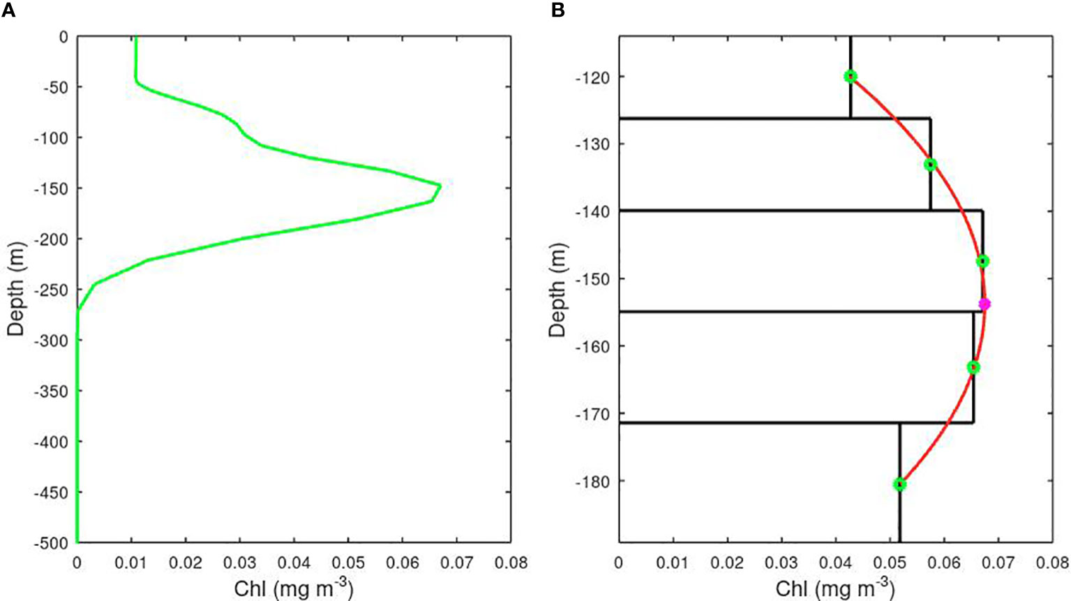
Figure 3 The precision of the depth of a model’s Deep Chlorophyll Maximum is improved by fitting a parabola to the values for the 5 layers bracketing the largest value. (A) The complete profile over 500 m. (B) Zoom in on the peak, with the derived depth of the peak shown by the pink asterisk. (Example is from MEDUSA’s representation of SSTG).
Figure 4 shows the chlorophyll concentration data for the SSTG from the ERSEM model. It is clear that the values at the DCM are an order of magnitude greater than at the surface, and that strong seasonal variations can be seen in both the depth of the DCM and in the concentration at the surface, with peak surface concentrations in May-June, although with significant interannual variation. The total column-integrated chlorophyll shows much weaker seasonal variations, with the annual modulation of the total being only about ±5% of the mean. A slight minimum occurs at the middle of the year, which is when the surface signature is strongest. However, that does not necessarily imply a causal connection, as the total chlorophyll could be responding to many different factors having a seasonal variation.
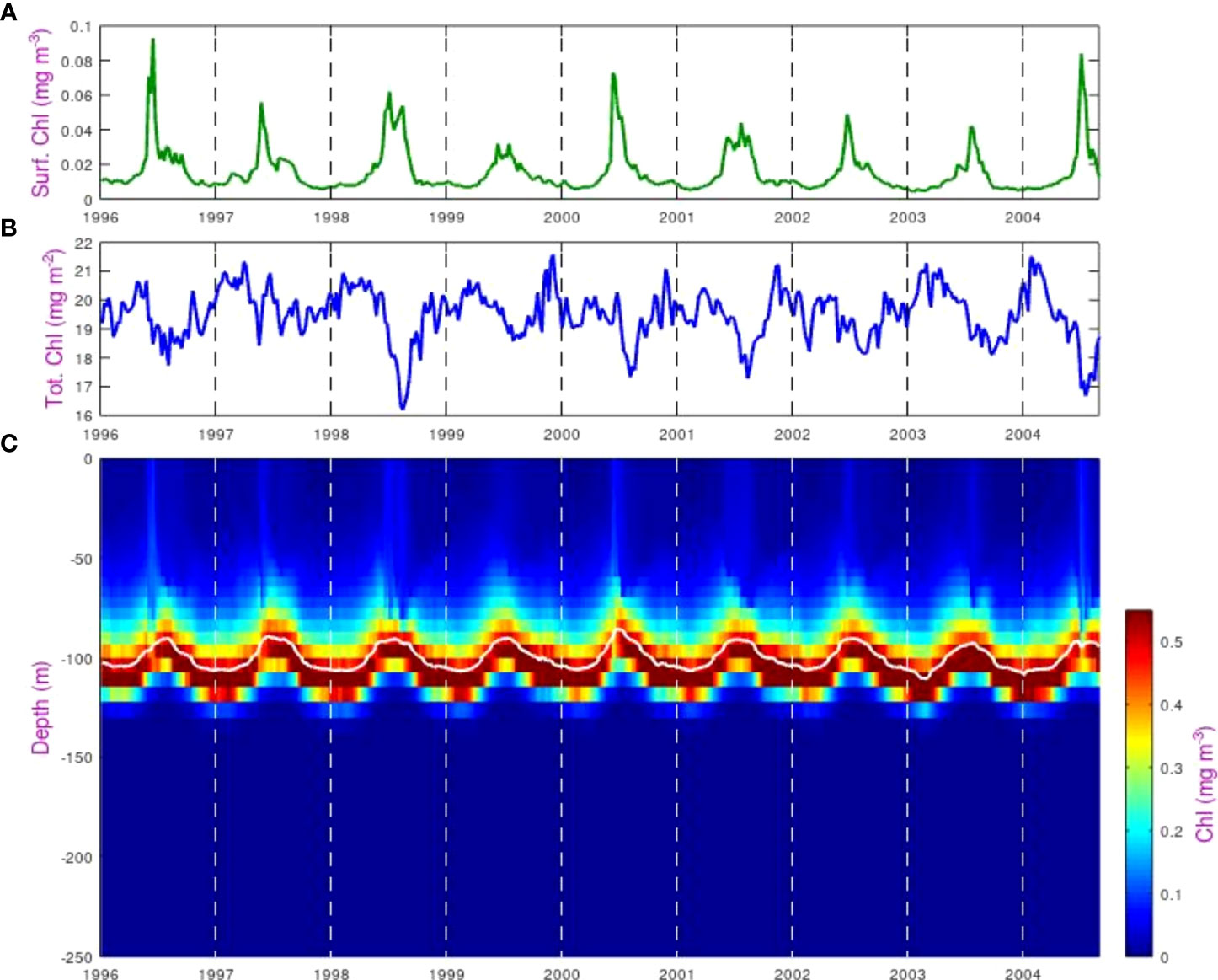
Figure 4 Variations in chlorophyll concentration at the SSTG within the ERSEM model. (A) Value in the surface layer, (B) Total column-integrated chlorophyll, (C) Value in each depth bin, showing the variation in depth of the DCM peak (highlighted by the solid white line).
3.3 Seasonal variations
Figure 5 shows the differences in mean values and seasonal variation for the various in situ datasets and for the numerical models. Although numerical biogeochemical models perform well at getting the broad patterns of surface chlorophyll variation correct (e.g. Figure 11 of Yool et al., 2011), it is often challenging to get the magnitudes correct. This is particularly the case at the extremes (highly productive and oligotrophic regions).
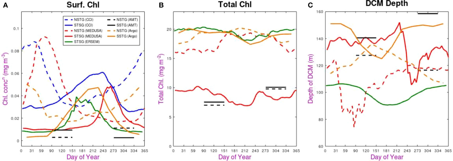
Figure 5 Seasonal variations in the various datasets. (A) chlorophyll concentration in the surface layer, (B) Total column integrated chlorophyll, (C) Depth of DCM. In all cases the solid line shows observation for the SSTG and the dashed line for the NSTG. The satellite (CCI) dataset only provides surface measurements, and the AMT data are simply shown as averages over the two distinct periods when the transects took place.
The surface chlorophyll concentration shows strong seasonal modulation for all the continuous datasets (both CCI and models), with that for the NSTG peaking in February-March and the SSTG reaching its maximum sometime between June and August. This agrees with prior satellite analysis by McClain et al. (2004) and Aiken et al. (2017). The timing of the AMT cruises puts them outside these periods of maximum surface chlorophyll, implying the cruises are not suitable for a detailed seasonal examination; however it does also mean that two or three weeks difference between the time of year of various cruises should not lead to apparent interannual variation.
The SSTG surface bloom for ERSEM occurs three months earlier than in MEDUSA, and also lasts longer. That evidenced by the satellite data has a peak slightly earlier than in MEDUSA and a much longer duration than in either model. A similar picture is seen for the NSTG: the heightened chlorophyll values in the CCI dataset peak a month earlier than in MEDUSA and have a longer duration. The temporal pattern revealed by BGC-Argo matches well that of CCI, but both in situ sources (AMT and Argo) have much lower values. This is possibly due to non-photochemical quenching, which is discussed later.
When considering total chlorophyll in the water column we note that there is no clear pattern. The two models disagree in the magnitude of the total for the SSTG by a factor of two, although both show slightly higher values for March-May (autumn) than for July-August (winter), so there is slightly less in total when values are higher in the surface layer, confirming this anti-correlation in seasonality noted by Hardman-Mountford et al. (2013). This pattern is clearer for MEDUSA’s representation of the NSTG, with ~20% more total chlorophyll outside the peak months for surface chlorophyll.
The values from BGC-Argo floats are of a very similar magnitude to those produced by the models, with the Argo-derived values at SSTG matching the seasonal variation shown by ERSEM and those for the NSTG being close to those for MEDUSA. However, that model has much lower values for the SSTG, which appear to be roughly matched with AMT values at both sites. All the datasets with year-round coverage show total chlorophyll to be at its smallest during the winter period for that site.
Finally, we consider the seasonal variations in the depth of the DCM. The value at any particular time may not fully reflect the state of the ecosystem, as physical features (e.g. eddies or internal waves) may raise or lower the level quite considerably. However, we use point values for DCM depth from the model rather than some large-scale average (see Appendix) because the in situ measurements are discrete point measurements. Figure 4 showed that for the SSTG ERSEM had a regular gently varying DCM depth; this translates into a smooth climatological signal varying around 100 m (Figure 5C), with a decrease at the time of the peak surface concentrations (typical of 1-D simulations). MEDUSA has a much wider variation of values, due to the physical features passing through, but on average the depth at the SSTG is much deeper (130-140 m). The decreases in DCM depth in MEDUSA both coincide with increased surface values. For the SSTG, the BGC-Argo profiles show a seasonal variation matching ERSEM, but with typical depth values agreeing with MEDUSA; Argo’s DCM depth variation for the NSTG is, as might be expected, roughly the reverse of that for the SSTG, whereas the MEDUSA variation is more complicated and less clearly linked to surface changes.
3.4 Interannual variations
Within the climatological means illustrated previously there is often a great range of individual values. Figure 6 shows probability distribution functions (p.d.f.) of the depth of DCM and the total columnar chlorophyll. In this case, data are shown separately for the two seasons for which AMT observations exist. As noted before ERSEM shows a shallower DCM than the other datasets, but does agree that for the SSTG the DCM is generally slightly higher in austral autumn than in spring. AMT and BGC-Argo also show a slightly higher DCM for NSTG in boreal autumn than in spring, but this is not the case for MEDUSA. In MEDUSA both spring sets of observations show a pronounced minority of shallow DCM events, possibly related to passing physical features having advected nutrients up from deeper layers (but also note the issue of spatial variation discussed in the Appendix).
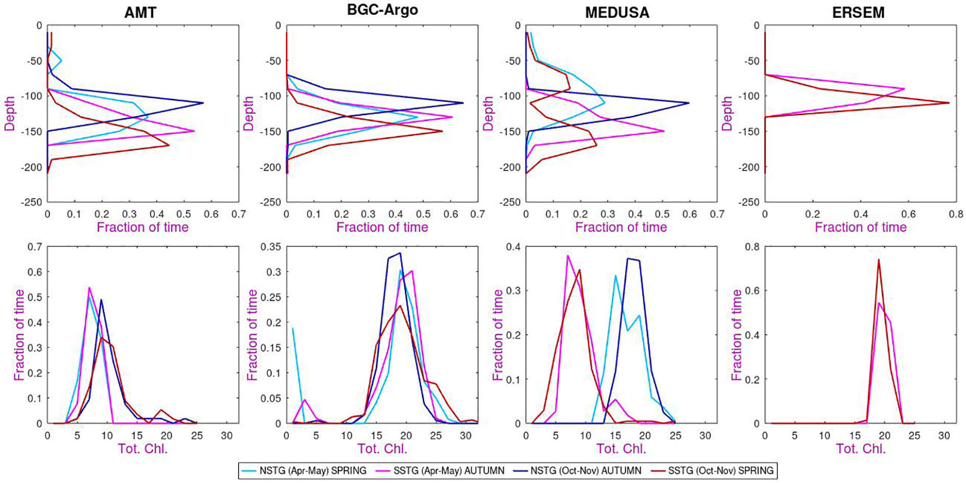
Figure 6 Probability distribution functions of (top row) depth of DCM (second row) total chlorophyll. The same colour legend applies to all panels. [The binning intervals are 20 m in depth (top row) and 2 mg m-2 for total chlorophyll (bottom row), with “fraction of time” indicating that all histograms are normalized to unity].
When considering the p.d.f.s of total chlorophyll (second row of Figure 6) we note that there is a large variation in the values. MEDUSA for SSTG and AMT for both sites yield values of order 10 mg m-2, but MEDUSA for NSTG and ERSEM and ARGO estimate the totals as of order 20 mg m-2. The spring/autumn variation is weak, with AMT and MEDUSA datasets showing increased values for both regions during Oct-Nov compared with Apr-May, whereas ARGO shows the reverse and for ERSEM the distributions for the two periods are similar. However the periods under consideration represent the transition times at the end or start of the peak surface chlorophyll period, and so the relative change between Apr-May and Oct-Nov is sensitive to when the surface values intensify in these datasets. We also note that the AMT Apr-May sections mainly occurred early in the programme, whereas Oct-Nov transects have taken place more evenly throughout the AMT programme (Figure 1), so the seasonal difference noted for AMT may partially reflect an increasing trend in surface chlorophyll noted in Figures 15 and 16 of Aiken et al. (2017).
Table 1 summarises the statistics describing the chlorophyll profiles in all four datasets. ERSEM has a much larger amplitude for the DCM peak than the other datasets; however as it’s DCM is typically shallower and less wide than in the other datasets, it returns a total chlorophyll value in line with most of the others. The seasonal change in amplitude of peak chlorophyll is generally opposite to that of the width of the DCM, so that the total chlorophyll has a weaker variation than either (see Figure 5B). Aiken et al. (2017) show output from the biological model of Brewin et al. (2017), which also gives values of total chlorophyll in the middle of the gyres of around 22 mg m-2, with a seasonal variation of only ~5%.
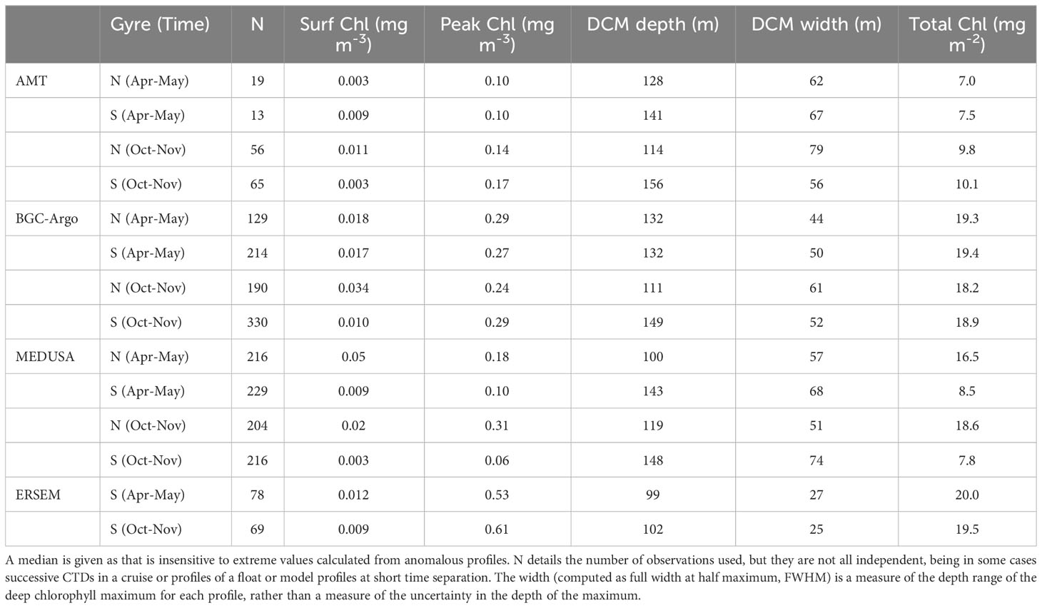
Table 1 Characteristics of the NSTG and SSTG chlorophyll profiles derived from the various datasets.
3.5 Significant connections?
A great many physical and biological properties exhibit a seasonal cycle so that significant correlations may be found, especially with the assumption that one value may lag another by several weeks. However, no causal connection should be inferred because each may be responding to different solar-related drivers e.g. cloudiness, sea temperature, windiness etc. However if we consider anomalies from the average for that time of year, then it may be more significant if some extreme of a surface value presages the variation at depth.
In Figure 7 we examine the co-occurrence of anomalies in surface chlorophyll with those in total chlorophyll or depth of DCM. The colour scheme reflects the four different sampling regimes, since the connection may not be the same for all such “modes”. Firstly we note that there is a great deal of scatter – once the regular seasonal variations are removed, there are potentially many causes for the weaker remaining variations, so that a connection between anomalies in surface and sub-surface properties will be much weaker. Conversely a unique event in the MEDUSA representation of the NSTG for Oct-Nov produced large anomalies in various properties leading to a significant correlation value without necessarily being indicative of a causal relationship occurring throughout the rest of the time series.
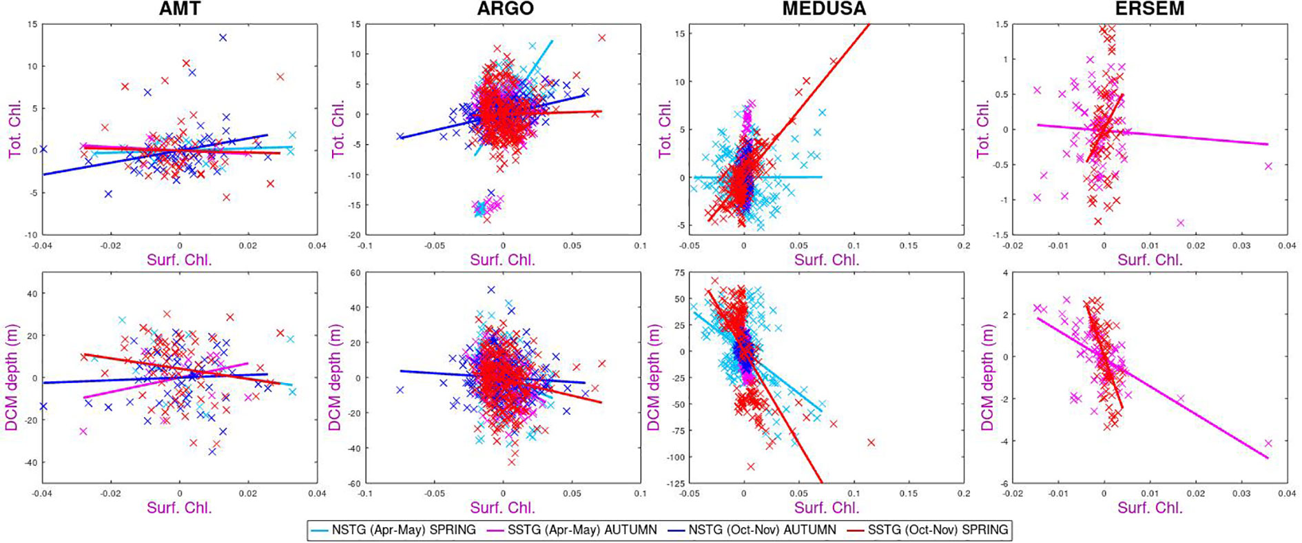
Figure 7 Correlation of anomalies in surface chlorophyll with values at depth, with no lag. The plot compares behaviour at NSTG and SSTG for the two parts of the year sampled by AMT. MEDUSA’s anomalies for the NSTG in Oct-Nov are dominated by one large event in the 18-year time series.
Assigning confidence intervals to these correlations is challenging, as consecutive CTD casts or Argo profiles will not be independent, so instead here we look for common themes spanning various datasets or common to both gyres for the same season.
Regions with enhanced upwelling tend to have lower SST but higher surface chlorophyll, due to nutrient supply, leading to negatively correlated spatial patterns of these two properties. Figure 8 shows that the year-to-year variation in these two surface terms are also usually negatively correlated, which would be consistent with changes in mixing affecting these two aspects coherently. However this is not borne out for AMT sampling of the NSTG. We hypothesise that this may be due to the wide variation in the route traversed in the northern hemisphere, especially during the first decade that provided most of the Apr-May transects. Thus a variation in the locations being compared may be the cause of the positive correlation noted between SST and surface chlorophyll. Similarly warmer than average SST tends to be associated with a shallower MLD and so a negative correlation, with the exception also being in the behaviour noted for the AMT observations of the NSTG.
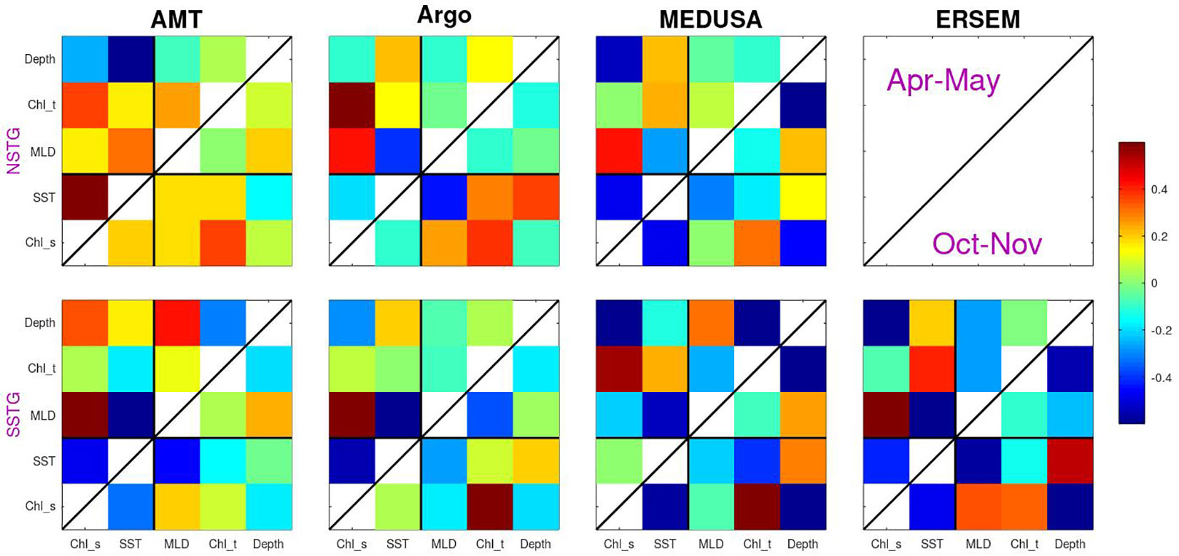
Figure 8 The correlation between various properties calculated using anomalies relative to the mean for that time of year. The values analysed comprise two surface properties (surface chlorophyll and SST) and three sub-surface values (MLD, total chlorophyll and depth of DCM), with the colour indicating the correlation. Analysis is for both gyres and the two periods sampled by AMT (with Apr-May above the diagonal line and Oct-Nov below it).
Continuing on to the sub-surface biological properties we note that both models show a strong negative correlation between amount of surface chlorophyll and the depth of the DCM. This is as expected due to increased surface chlorophyl reducing the amount of PAR reaching depth. However, this expectation is not borne out by the AMT measurements of one of the modes (SSTG in Apr-May), which instead shows a high positive correlation. The surface chlorophyll value is generally positively correlated with the columnar total, however for the SSTG in Apr-May three of the datasets (AMT, Argo and ERSEM) agree that the correlations are close to zero.
With regards to the overall pattern of correlations shown in Figure 8, there is a good correspondence between those for MEDUSA and ERSEM. Both are, of course, numerical models and thus can only show patterns corresponding to the result of those biogeochemical interactions that have been modelled. However they are very different models, with MEDUSA being a full 3-D fine resolution grid with features being advected through and ERSEM being a 1-D implementation of conditions in the SSTG, but with more nuanced biological components. The analysis of the AMT data shows some agreement with that from analysing the models, but there are many differences. These could be due to the real world having interannual variations in forcing conditions or biological interactions not simulated in the models; however it could also be partially due to the Apr-May occupations being principally in the first half of the period analysed in the models and there also being much spatial variation in the tracks occupied then, so complicating the calculation of anomalies in various properties.
3.6 Delayed response?
In winter PAR is lowest, and the reduced light flux to the DCM results in reduced growth of phytoplankton there. Consequently the nutrient gradient enables more nutrients to be entrained into the sub-surface mixed layer above the DCM, increasing chlorophyll values near the surface. A positive feedback can be established, with the increased chlorophyll production at the surface further reducing light flux to the DCM and so enhancing surface production. As the seasons progress from low-light winter to spring the higher PAR flux penetrates to the DCM, increasing chlorophyll production there and cutting down the nutrient flux to the surface. [Letelier et al. (2004) note that for the NSTG in the Pacific, the isolumes (contours of equal illumination) are displaced by as much as 31m between winter and summer].
For the biological response, the chlorophyll signal at depth may possibly lag behind the changes at the surface, if there is vertical variability in growth and loss rates between layers. Alternatively, if most of the anomalies (relative to the average for that time of year) are due to mesoscale features advecting through, then the changes at surface and depth are likely to be coherent. To investigate these issues we explore the correlation between anomalies in surface and sub-surface features, looking at lags of the order of weeks.
For the AMT sub-surface measurements there are no in situ samples a few weeks prior to the CTD casts, so the AMT estimates of the DCM have to be contrasted with earlier satellite observations of the surface from the CCI project (Figure 9). These satellite-derived products have been well-validated on AMT (Brewin et al., 2016; Tilstone et al., 2021). The dataset being used provided 5-day composites every 5 days, so we investigate lags from 0 to 25 days. The MEDUSA model had a time step of 5 days and ERSEM was at steps of 7 days, so these were used in the lag analysis. Only positive lags were considered, as we do not expect the sub-surface changes to lead those at the surface.
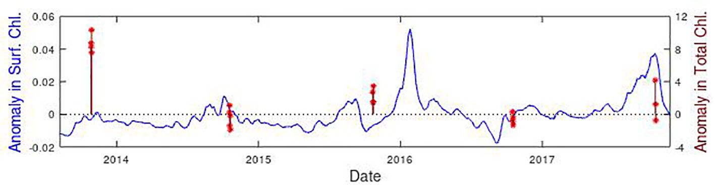
Figure 9 Time series of surface chlorophyll concentration at the SSTG observed by CCI (in blue) and AMT estimates of total chlorophyll (in dark red). Both datasets are expressed as anomalies relative to the mean value for that time of year, with 4 or 5 independent CTDs taking place within the specified region for each cruise. Note both datasets cover 2001-2020, with this panel simply providing a zoom to show the details.
Figure 10 shows the results of the lag analysis, indicating to what degree prior information on surface chlorophyll concentrations could be used to predict either total depth-integrated chlorophyll or the depth of the DCM. For total chlorophyll. the correlations are of order ±0.25. MEDUSA shows similar patterns for NSTG and SSTG, with a negative response in Apr-May peaking at ~15 days, whilst there is a positive correlation in Oct-Nov that is maximum at zero lag. This is surprising given these periods correspond to different community growth/decline conditions at the two sites. For the SSTG, ERSEM also shows a positive correlation but peaking at ~14 days.
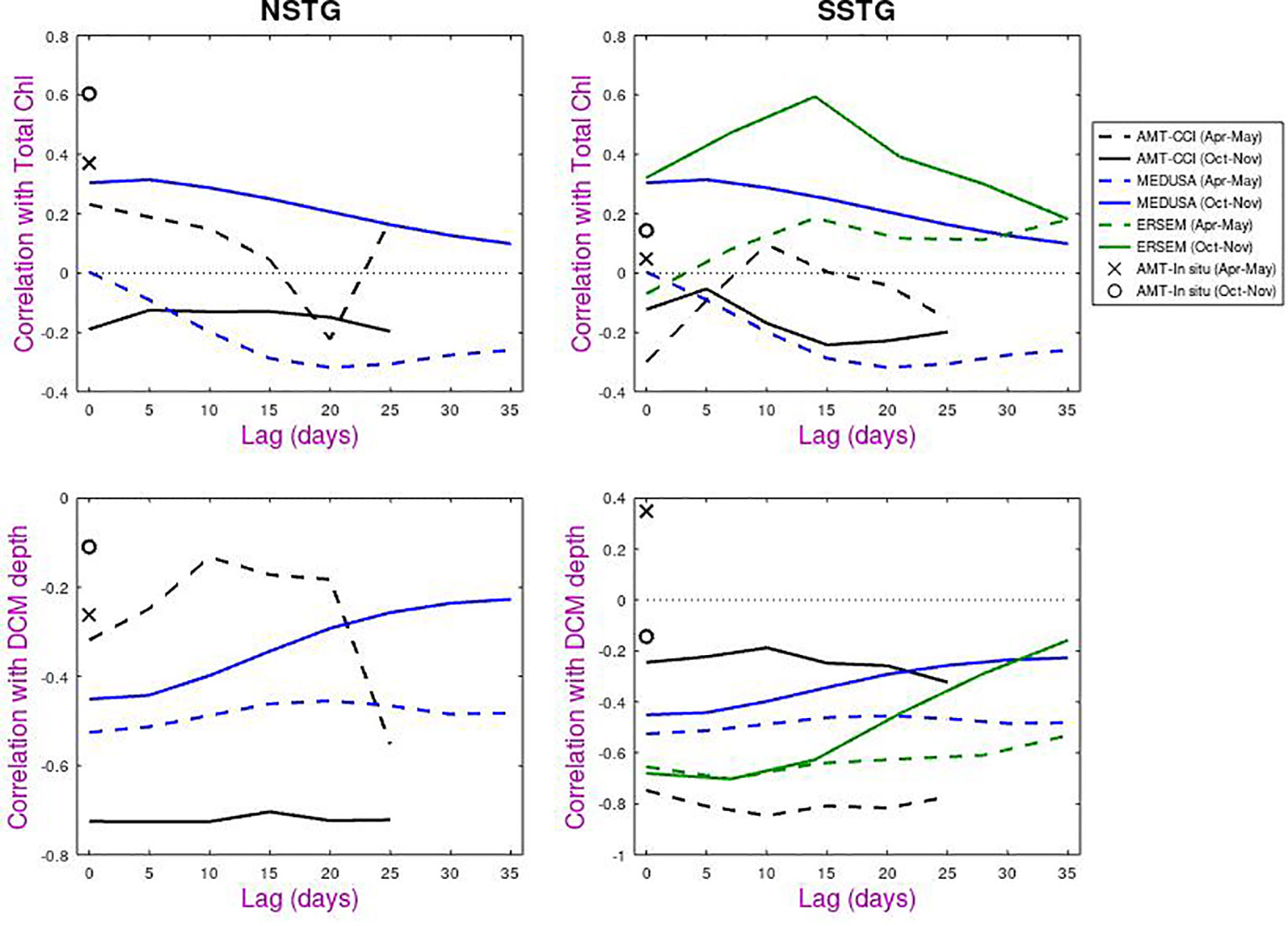
Figure 10 Lagged correlations of total chlorophyll and depth of DCM against surface chlorophyll measurements for all datasets (AMT, MEDUSA, ERSEM) on the same axes. Dashed lines and cross are for Apr-May and solid lines and circle are for Oct-Nov.
Larger correlations are noted for the DCM depth and they are nearly all negative. One particular point of interest is the low correlation for AMT with in situ measurements of surface chlorophyll, but high correlations (approaching -0.8 for autumn) when compared with satellite-derived chlorophyll. The low values for the in situ comparison are probably due to non-photochemical quenching i.e that plankton in the sunlit ocean have adjusted their chlorophyll response to dissipate excess energy and thus give a low response to fluorometers. (More accurate values of in situ chlorophyll can be obtained by HPLC of collected samples, but these are only available for discrete depths).
Whilst the AMT-CCI analyses for the two gyres show similar response for boreal and austral autumn and also for boreal and austral spring, both models tend to show a flat response for Apr-May for NSTG and SSTG, and a response that peaks at zero lag for Oct-Nov. These flat responses may indicate that the DCM depth in the models is not so much responding to the amount of surface chlorophyll present at that time, but to the underlying environmental conditions that have led to that year having more or less surface chlorophyll than normal.
4 Discussion and conclusions
4.1 Seasonality observed by in situ sensors
The biogeochemical monitoring of the Atlantic through the Atlantic Meridional Transect programme has been ongoing for almost 30 years. There are many individual research cruises that sample some highly productive Longhurst province during a major bloom, but AMT is unprecedented in its deliberate inclusion of measurements in the centre of the Atlantic’s subtropical gyres. Although these regions are much lower in chlorophyll concentration, they are of large expanse. Models and BGC-Argo profiles show that there is seasonality within these gyres, with variation not only at the surface but also at depth. However for logistical reasons the AMT cruises have always been in April-May or October-November (with most cruises in the last decade in the latter interval) and so the seasonal variation cannot be easily explored from these hydrographic measurements. On the other hand, the sampling at these times of year better enables long-term trends to be analysed, compared with the variation between midwinter and midsummer.
Profiles from drifting biogeochemical Argo floats offer some insight into the seasonal variations at depth in the real ocean. For the SSTG, there is a simple near-sinusoidal variation in the average depth of the deep chlorophyll maximum, and in the total column-integrated chlorophyll, with the minimum in the middle of the year coinciding with the peak in surface chlorophyll. For the NSTG, BGC-Argo shows a minimum in depth of DCM and in total chlorophyll for November-February; which mirrors Argo’s observation of surface properties, and aligns with the temporal variation of the CCI product (Figure 5A). However the satellite product yields values consistently higher than our in situ estimates.
HPLC measurements are usually considered as the most trustworthy records of chlorophyll concentration. HPLC data for 3 recent AMT cruises suggest the low values in the centre of the gyres are only about 0.04 mg m-3 (Figure 2 of Tilstone et al., 2021). As stated in the data description (sections 2.1 and 2.2), the chlorophyll profiles recorded by AMT’s CTD casts and the BGC-Argo floats do not always go to zero at depths below 250 m, but have small values both positive and negative. This has been interpretted here as a slight offset in the sensor calibrations and this deep value subtracted from the whole profile. However there may be a real small bias, where there is actually some fluorescence from detrital particles, non-viable phytoplankton and coloured dissolved organic matter (Xing et al., 2017). This could explain why the AMT and Argo values for surface chlorophyll are smaller than most other records, including the CCI data from satellites. A reduction in the base value subtracted from each whole profile would also lead to an increase in the columnar total. Brewin et al. (2017) also suggest that total chlorophyll values calculated from AMT’s water samples yield a higher value than those calculated from the fluorometer alone. Analysis of flow cytometry data for two earlier AMT cruises showed that the dominant plankton in such nutrient-depleted waters was Prochlorococcus, and also showed that the DCM peak was ~0.1 mg m-3, with its depth being deeper for the SSTG than NSTG (see Figure 3 of Tarran et al., 2006), in keeping with our fluorometer analysis detailed in Table 1.
4.2 Oligotrophic gyres in numerical biogeochemical models
Although numerical biological models can readily produce the spatial patterns of chlorophyll variation (e.g. Figure 11 of Yool et al., 2011), as that is modulated by the physics, achieving the correct magnitudes is more challenging. This is particularly so in low productivity regions, where some models may implement tuning or use non-linear loss rates in order to enable a standing stock of phytoplankton to overwinter without dying out. There may also be issues with supply of nutrients at the base of the mixed layer, as such effects have to be parameterised to allow for submesoscale physical processes that are not resolved by typical basin- or global-scale models. Many authors (e.g. Figure 1 of Signorini et al., 2015) have shown the regions of low surface chlorophyll and the presence of a DCM are linked to regions with a deep nitracline, with the resupply of nutrients from below being essential for the maintenance of these sub-surface features.
Both ERESM and MEDUSA produce a clear sub-surface chlorophyll maximum, but in the case of the 1-D run of ERSEM this is well-constrained to depths in the range 90-110 m (see Figure 4), with a peak concentration at depth of ~0.6 mg m-3, leading to a total chlorophyll of ~20 mg m-2 (Figure 5B) that is much higher than noted by AMT’s CTD data. The large peak values in the DCM are partially offset by the narrowness of the sub-surface chlorophyll peak (~25 m, see Table 1), which may suggest insufficient vertical diffusion of nitrates in the model. ERSEM also shows the simple seasonal variation borne out by the BGC-Argo analysis.
For the SSTG, MEDUSA produces a DCM at ~120-150 m with a width of ~70 m (FWHM), more in keeping with the AMT and Argo values, and its associated total chlorophyll is only 10 mg m-2, agreeing broadly with AMT (but not Argo). For the NSTG, it has a shallower DCM with a higher chlorophyll concentration at its peak (0.2 mg m-3, as opposed to 0.1 mg m-3 for SSTG), leading to a significantly higher total chlorophyll. In portraying the NSTG as having a shallower DCM, higher total chlorophyll and higher surface chlorophyll than the SSTG, MEDUSA agrees with the differences noted for both AMT and Argo.
Figure 11 of Aiken et al. (2017) show that the model of Brewin et al. (2017) produces a DCM at a depth of 85-95 m (in keeping with ERSEM) for both gyres, with values shallower in the winter period. That model also gives values of total chlorophyll of ~22 mg m-2, with peaks in the winter at the time of highest surface concentration. The standard run of the COBALT biogeochemical model gave DCM depths of ~85 m in NSTG and ~60 m in SSTG, with Moeller et al. (2019) modelling grazing as a diminishing function of light intensity in order to get depths of ~135 m i.e. close to that observed in situ. Given their large spatial extent, it is crucial that models are able to portray the DCM accurately. MEDUSA appears to be one of the earliest global biogeochemical models to get the depths correct and also the integrated total for the NSTG. However the intensity of the peak for the SSTG is too weak – further work should look at the factors affecting both nutrient supply and losses in this region.
4.3 Connections between surface and sub-surface
There are many factors that affect the strength and location of the deep chlorophyll maximum within these gyres. Eddies migrating through these regions may raise or lower isopycnal surfaces, which can in turn affect the DCM. Cornec et al. (2021) noted that cyclonic eddies can provide the conditions for enhanced growth leading to a “deep biomass maximum”, whereas anticyclonic eddies forcing the plankton down encourage increased chlorophyll production within the plankton (“deep photoacclimation maximum”) in order to harvest enough light. However by collating data from a large number of CTD stations and BGC-Argo profiles we hope to average over such effects, but these transient phenomena will reduce the observed correlations.
The majority of other environmental factors have a direct or indirect link to the annual cycle of solar irradiation e.g. solar zenith angle, stratification, wind fields, cloudiness, and so it is expected that there will be seasonal cycles in SST, mixed layer depth, surface chlorophyll, depth of DCM and total chlorophyll. Some of these conditions, such as SST, will lag the solar cycle, so not all properties will peak at the same time. To get some insight into causal connections we have examined anomalies in various properties relative to their means for that time of year.
The seasonal cycles of SST are not shown, but, in general, northern hemisphere sites (including NSTG) will peak in Sept-Oct, and southern ones in Mar-Apr. Thus cool SST values partially precede the annual decrease in DCM depth (Figure 5C). Examination of anomalies relative to the seasonal average shows that higher than normal SST values are generally associated with a shallower than normal mixed layer, but with a deeper DCM. (The exception is the AMT observations of the NSTG, where the diversity of routes, as shown in Rees et al. (2015), may be a major factor.) The observed correlations could be related to reduced levels of surface chlorophyll that allow light to penetrate slightly deeper and promote the DCM, or to shallower mixing being unable to entrain higher nutrient concentrations at depth and nutrient-starving the surface. This is another question that could benefit from extended investigation with model simulations, especially as models permit individual processes such as mixing and diffusion to be selectively turned off in order to ascertain their impact.
The seasonal cycle of total column-integrated chlorophyll only varies slightly (~10%), with its minimum and that for the depth of the DCM occurring roughly when the surface chlorophyll is a maximum (Figure 5). However, when considering interannual variations, increased surface chlorophyll is associated with a shallower DCM, but is positively correlated with increases in total chlorophyll (Figure 8). SST also appears to be negatively correlated with DCM depth in Apr-May but positively correlated in Oct-Nov for both NSTG and SSTG, indicating that different factors are relevant in the two locations.
Some of the strongest correlations are between surface chlorophyll and the depth of DCM, with increased surface concentrations leading to a shallower DCM, as noted by others e.g. McClain et al. (2004). Mignot et al. (2011) collated observations from many geographically diverse regions and showed a high correlation (r2 = 0.81), whilst Mignot et al. (2014) showed this connectivity between surface chlorophyll and DCM depth for 4 individual BGC-Argo floats monitoring the seasonal cycle in 4 separate low productivity regions. Similarly, Uitz et al. (2006) have shown a positive correlation between surface and depth-integrated chlorophyll values, with their selection of stratified waters having a large spatial variation and encompassing a wide range of surface chlorophyll values. We have extended those observations to interannual timescales, showing that once seasonal cycles are removed there is still a clear anti-correlation i.e. that an exceptionally strong surface signal leads to a less pronounced and shallower DCM than normal.
This is particularly pronounced for satellite observations of surface chlorophyll with AMT measurements of DCM depth during boreal and austral autumn (Figure 10), with the connection being much weaker in the spring seasons. The lagged correlations in Figure 10 show that the effects of anomalies in surface chlorophyll on the DCM persist for many weeks. This suggests that satellite observations can provide some skill in predicting sub-surface conditions in at least some seasons. AMT does not provide observations for winter or summer, but as the models show reasonable agreement for the DCM depth in the SSTG, it may be fruitful to consider what correlations they offer in those seasons.
At present it is not clear if this is just a biological response, or whether physical factors (such as slowly passing eddies or Rossby waves) are causing coherent variations in these measures of biology. A much more expansive analysis of MEDUSA could address this issue by studying a much wider spatial extent than used here and assessing and, if necessary, removing the effect of eddies to leave the biological response of a quiescent ocean.
4.4 Use of chlorophyll concentration as a proxy for biomass
Throughout this paper we have used estimates of chlorophyll as an indicator of biomass. Although widely used for pragmatic reasons (see Table 1 of Sathyendranath et al., 2023), there are potential biases arising from assuming a simple correspondence between chlorophyll and biomass.
Firstly, the chlorophyll to carbon (or mass) ratio varies with individual species. As different ecological niches favour different plankton functional types there will be changes in this ratio, both laterally and vertically. Figure 4C of Graff et al. (2016) displays the change in the ratio for surface waters, with the oligotrophic gyres being marked by chlorophyll content being less than half of that in other regions. Tarran et al. (2006) and Heywood et al. (2006) noted that picoeukaryotes were the most abundant plankton group within these gyres and also contributed the most biomass in the DCM. Of these, Prochlorococcus is far more abundant than Synechoccus (Zubkov et al., 1998), so even though the latter has a greater size and thus fluorescence per cell its contribution to the overall chlorophyll signal remains small (van den Engh et al., 2017).
Secondly, many plankton groups respond to low-light conditions by increasing the concentration of chlorophyll within them. Such photoacclimation processes typically occur within a few hours (Lewis et al., 1984), so the biological community readily adapts to environmental changes as internal waves or eddies propagate through the region. These changes mean that for an individual species within these gyres the pigment to particle volume ratio increases with depth towards the DCM and then stabilises or decreases below that (Kitchen and Zaneveld, 1990; Fennel and Boss, 2003). However, Figures 6 and 7 of van den Engh et al. (2017) show that the DCM in the North Pacific oligotrophic gyre does correspond to both a peak in abundance of Prochlorococcus as well as in its fluorescence signal. The increase in chlorophyll is not always marked by a proportional increase in fluorescence due to “packaging”, which describes the degree to which chlorophyll concentration within the cell affects its ability to absorb light and then fluoresce (Cullen, 1982). However the strong diurnal mixing present in these calm low-latitude regions implies a degree of uniformity within the small standing stock present in the seasonal mixed layer, and thus a less pronounced photoacclimation change near the surface.
Chlorophyll is the common currency for these comparisons of models and observations. Whilst the variable stoichiometric ratios used by the ERSEM model enables it to accommodate photoacclimation, the model output that we have obtained only corresponds to chlorophyll. Many of the AMT cruises have obtained water samples at various depths throughout the transect, but their vertical resolution is coarse. The BGC Argo floats, however, do offer an alternative high-resolution record of plankton through measurement of backscatter at 700 nm (different from the wavelength used for the fluorescence response). This normalised backscatter, termed bbp700, is often related to the concentration of particulate organic carbon (POC), which is an amalgam of phytoplankton, zooplankton, detritus and other non-viable material, and thus can be difficult to interpret solely as an index of phytoplankton biomass. It is also not a variable directly reproduced by most ecosystem models and thus not the focus of this study. Nonetheless future work could make use of these data for testing how well ecosystem models can reproduce photoacclimation processes. The backscatter for phytoplankton corresponds to their cross-sectional area, rather than their chlorophyll content.
A typical bbp700 profile within these gyres is shown in Figure 11. The backscatter is fairly constant above the DCM, beyond which it decreases to its noise floor for deep waters. The values in the top 150 m are due to a range of particulates, many of which lack a fluorescence signal. These could be detritus or plankton in a non-active state due to nutrient depletion. We extracted the depth at which bbp700 values reduced to midway between surface and deep values and compared that with the depth below the DCM where chlorophyll fluorescence values were halved. The two measures were correlated (r2 = 0.42 for NSTG, r2 = 0.56 for STSG) but we did not feel these represented a useful measure of biological depth, as the bbp700 value was always lower and may simply indicate a physical feature such as the depth of maximal vertical stability noted in Figure 9 of Agusti and Duarte (1999).
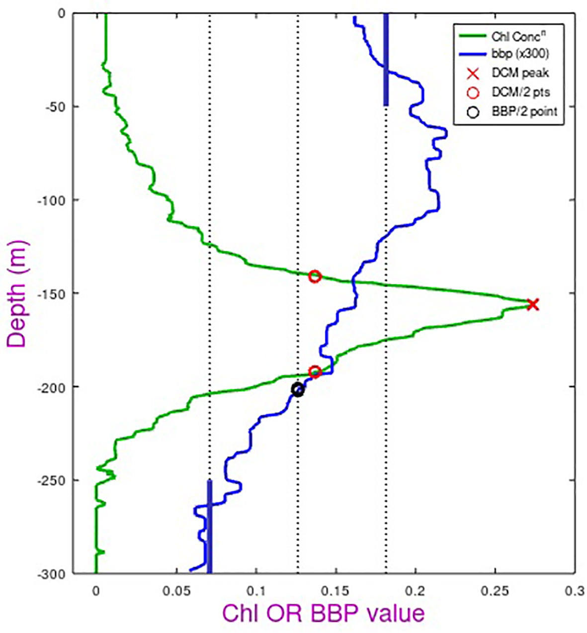
Figure 11 Schematic showing the definitions of the bottom depth of the biomass layer (note backscatter values have been multiplied by 300 to allow them to be displayed on the same scale). Chl-a (in mg m-3) is derived from fluorescence, with a peak value and locations of half peak concentration (red circles) defined. BBP (in m-1) is the optical backscatter observed at 700 nm wavelength. After despiking and application of a median filter, average surface and deep values are defined (thick blue bars) and the depth with the backscatter value midway between these selected (black circle).
An attendant issue is the assumption of proportionality between chlorophyll content and fluorescence response, which is the basis for fluorometer measurements from AMT and BGC-Argo. Petit et al. (2022) note that there are two main factors affecting the fluorescence yield: the light level and the fluorescence quantum yield of the particular phytoplankton present. In near-surface waters plankton may produce auxiliary pigments to reduce the radiation being absorbed by the chlorophyll and thus preventing heat stress to the organism. (Note, the CHLA_ADJUSTED field of the Argo data had already had a correction applied for non-photochemical quenching). Figure 2 of Petit et al. (2022) shows that chlorophyll estimation via fluorescence compared with HPLC analysis can vary by a factor of six, with the fluorometers significantly overestimating for communities of micro- rather than the smaller nano- and pico-plankton. As the oligotrophic gyres are dominated by the smaller classes of plankton throughout the water column, this effect, associated with plankton community structure, does not affect this study, but could be an important issue for more productive locations with a changing size population through the water column.
The work of Roesler et al. (2017) suggests that the fluorometer-derived chlorophyll estimates from BGC-Argo floats should not simply be corrected by a uniform factor everywhere; however, there is, as yet, no spatially-varying correction that is robust enough for the standard processing chain (Catherine Schmechtig, pers. comm., 2023). The data in Table 2 of Roesler et al. (2017) suggest the correction factor should be 50% larger for SSTG than NSTG, which would reduce the chlorophyll estimates of the former (surface, peak of DCM and integrated value) by a third. If implemented this would increase the disparity between the NSTG and SSTG. Likewise, the fluorometer calibrations for each AMT cruise are determined on a cruise-wide basis, since there are too few measurements to explore any regional variation in the fluorescence-chlorophyll relationship.
Thus, although there are reservations about the use of chlorophyll fluorescence as a proxy for phytoplankton biomass, we note that in these oligotrophic gyres the effects of depth-varying community structure and photoacclimation do not mask the development of deep concentrations of certain species such as Prochlorococcus, and that other sensors such as optical backscatter fail to shed adequate light on this phenomenon.
5 Overall summary
The AMT programme has generated a long-term dataset of surface and sub-surface measurements through many Longhurst provinces, with its repeated sampling within the oligotrophic gyres being almost unique. These ecosystems are representative of the ocean’s largest ocean biome by area, and exhibit characteristic deep chlorophyll maxima at depths > 100m where nutrient concentrations are high enough to support primary production. These AMT data enable us to establish that the DCM for the STSG (NSTG) lies at ~145m (~120m), and is slightly deeper in the spring season than autumn for that hemisphere. As AMT only sampled two periods in the year, data from the BGC-Argo array are needed to elucidate the full annual cycle, confirming that seasonally the DCM is shallowest around the months of highest surface concentration. Interannual variations echoed this with higher than normal surface values coinciding with a shallower than normal DCM. Lagged correlations showed considerable persistence of this effect. This paper also demonstrated how AMT provides an effective dataset for validation of the portrayal of oligotrophic gyres in biogeochemical models, opening the door to exploration of the underlying biological dynamics of these regions using the models that best represent them.
This investigation focussed on the permanently stratified regions in the Atlantic, due to the availability of long time series of data within them. However, it is expected that the chlorophyll characteristics found here for these Atlantic subtropical gyres will also be manifest in the equivalent gyres in the North and South Pacific and in the South Indian Ocean. A potential extension of this work would be to explore surface/sub-surface relationships in the seasonally stratified temperate gyres found poleward of the subtropical gyres, since once the “spring bloom” has exhausted the surface nutrients a DCM develops persisting throughout summer and autumn until convectional mixing resumes. As these regions enjoy episodic (annual) injections of nutrients rather than just slow upward mixing, the relationships in these regions may be subtly different.
Data availability statement
The data collected during the Atlantic Meridional Transect programme are hosted at https://www.bodc.ac.uk/data/hosted_data_systems/amt/ and the 5-day composites of satellite-derived chlorophyll were from the ESA CCI programme, with the earlier (v5) dataset available at https://www.oceancolour.org. BGC-Argo data were obtained from https://biogeochemical-argo.org/data-access.php. These data were collected and made freely available by the International Argo Program and the national programs that contribute to it. (https://argo.ucsd.edu, https://www.ocean-ops.org). The Argo Program is part of the Global Ocean Observing System. The files containing the selected model output can be obtained from the author upon request.
Author contributions
The original research concept was by JA, with GQ expanding the aims. GQ carried out all the research, produced the figures and wrote the original draft. This was modified in response to ideas and comments from all authors. All authors contributed to the article and approved the submitted version.
Funding
The author(s) declare financial support was received for the research, authorship, and/or publication of this article. The work was supported by UK Natural Environment Research Council (NERC) National Capability funding for AMT to Plymouth Marine Laboratory, with the time for Graham Quartly also supported by funding from the National Centre for Earth Observation (NCEO) and European Union’s Interreg Atlantic Area programme (grant agreement EAPA_165/2016 of the project iFADO: Innovation in the Framework of the Atlantic Deep Ocean). AMT is funded by the NERC through its National Capability Long-term Single Centre Science Programme, Climate Linked Atlantic Sector Science (grant number NE/R015953/1). This study contributes to the international IMBER project, the work of NCEO and is contribution number 399 of the AMT programme. RB is supported by a UKRI Future Leader Fellowship (MR/V022792/1).
Acknowledgments
We thank Arnold Taylor for insightful discussions to prompt this study. We are grateful to the many people who have helped make the data available: John Stephens and Tim Smyth for collecting and collating all the AMT CTD data and Luca Polimene for providing the ERSEM output, and acknowledge the help provided by Glen Tarran and Shubha Sathyendranath in understanding the plankton community structure and the role of auxiliary pigments. We acknowledge the support of NEODAAS for the data storage and processing resources.
Conflict of interest
The authors declare that the research was conducted in the absence of any commercial or financial relationships that could be construed as a potential conflict of interest.
The reviewer JB declared a shared affiliation with the author RB to the handling editor at the time of review.
Publisher’s note
All claims expressed in this article are solely those of the authors and do not necessarily represent those of their affiliated organizations, or those of the publisher, the editors and the reviewers. Any product that may be evaluated in this article, or claim that may be made by its manufacturer, is not guaranteed or endorsed by the publisher.
References
Agusti S., Duarte C. M. (1999). Phytoplankton chlorophyll a distribution and water column stability in the central Atlantic Ocean. Oceanologica Acta 22 (2), 193–203. doi: 10.1016/S0399-1784(99)80045-0
Aiken J., Brewin R. J. W., Dufois F., Polimene L., Hardman-Mountford N. J., Jackson T., et al. (2017). A synthesis of the environmental response of the North and South Atlantic Sub-Tropical Gyres during two decades of AMT. Prog. Oceanogr. 158, 236–254. doi: 10.1016/j.pocean.2016.08.004
Baretta J. W., Ebenhöh W., Ruardij P. (1995). The European regional seas ecosystem model, a complex marine ecosystem model. Netherlands J. Sea Res. 33, 233–2246. doi: 10.1016/0077-7579(95)90047-0
Brewin R. J. W., Dall'Olmo G., Pardo S., van Dongen-Vogels V., Boss E. S. (2016). Underway spectrophotometry along the Atlantic Meridional Transect reveals high performance in satellite chlorophyll retrievals. Rem. Sens. Env. 183, 82–97. doi: 10.1016/j.rse.2016.05.005
Brewin R. J. W., Tilstone G., Cain T., Miller P., Lange P., Misra A., et al. (2017). Modelling size-fractionated primary production in the Atlantic Ocean from remote-sensing. Prog. Oceanogr. 158, 130–149. doi: 10.1016/j.pocean.2017.02.002
Burchard H., Bolding K., Villareal M. (1999). GOTM: a general ocean turbulence model. Theory, applications and test cases (Brussels, Belgium: European Commission). Available at: https://www.researchgate.net/publication/258127949_GOTM_a_general_ocean_turbulence_model_Theory_implementation_and_test_cases (Accessed 16 Mar 2023). Technical Report EUR 18745 EN.
Clark D. R., Rees A. P., Ferrera C. M., Al-Moosawi L., Somerfield P. J., Harris C., et al. (2022). Nitrite regeneration in the oligotrophic Atlantic Ocean. Biogeosci 19, 1355–1376. doi: 10.5194/bg-19-1355-2022
Cornec M., Claustre H., Mignot A., Guidi L., Lacour L., Poteau A., et al. (2021). Deep chlorophyll maxima in the global ocean: Occurrences, drivers and characteristics. Glob. Biogeo. Cycles 35, e2020GB006759. doi: 10.1029/2020GB006759
Cullen J. J. (1982). The deep chlorophyll maximum: Comparing vertical profiles of chlorophyll a. Can. J. Fish Aquat. Sci. 39 (5), 791–803. doi: 10.1139/f82-108
Fennel K., Boss E. (2003). Subsurface maxima of phytoplankton and chlorophyll: Steady-state solutions from a simple model. Limn. Oceanogr. 4, 1521–1534. doi: 10.4319/lo.2003.48.4.1521
Graff J. R., Westberry T. K., Milligan A. J., Brown M. B., Dall’Olmo G., Reifel K. M., et al. (2016). Photoacclimation of natural phytoplankton communities. Mar. Ecol. Prog. Ser. 542, 51–62. doi: 10.3354/meps11539
Hardman-Mountford N. J., Polimen L., Hirat T., Brewin R. J. W., Aiken J. (2013). Impacts of light shading and nutrient enrichment geo-engineering approaches on the productivity of a stratified, oligotrophic ocean ecosystem. J. R. Soc Interface. 10, 9. doi: 10.1098/rsif.2013.0701
Heywood J. I., Zubkov M. V., Tarran G. A., Fuchs B. M., Holligan P. M. (2006). Prokaryoplankton standing stocks in oligotrophic gyre and equatorial provinces of the Atlantic Ocean: evaluation of inter-annual variability. Deep Sea Res. II 53 (14), 1530–1547. doi: 10.1016/j.dsr2.2006.05.005
Kitchen J. C., Zaneveld J. R. V. (1990). On the noncorrelation of the vertical structure of light scattering and chlorophyll α in case I waters. J. Geophys. Res. 95 (C11), 20237–20246. doi: 10.1029/JC095iC11p20237
Letelier R. M., Karl D. M., Abbott M. R., Bidigare R. R. (2004). Light driven seasonal patterns of chlorophyll and nitrate in the lower euphotic zone of the North Pacific Subtropical Gyre. Limnol. Oceanogr. 49 (2), 508–519. doi: 10.4319/lo.2004.49.2.0508
Levitus S. (1982). Climatological atlas of the world ocean (Rockville, Md, USA: NOAA Professional Paper 13).
Lewis M. R., Cullen J. J., Platt T. (1984). Relationships between vertical mixing and photoadaptation of phytoplankton: Similarity criteria. Mar. Ecol. Prog. Ser. 15 (1-2), 141–149. doi: 10.3354/meps015141
Madec G., and NEMO team. (2015). NEMO ocean engine. Available at: https://www.nemo-ocean.eu/wp-content/uploads/NEMO_book.pdf (Accessed 13 Mar. 2023).
McClain C. R., Signorini S. R., Christian J. R. (2004). Subtropical gyre variability observed by ocean-color satellites. Deep Sea Res. 51, 281–301. doi: 10.1016/j.dsr2.2003.08.002
Mignot A., Claustre H., D’Ortenzio F., Xing X., Poteau A., Ras J. (2011). From the shape of the vertical profile of in vivo fluorescence to Chlorophyll-a concentration. Biogeosciences 8 (8), 2391–2406. doi: 10.5194/bg-8-2391-2011
Mignot A., Claustre H., Uitz J., Poteau A., D'Ortenzio F., Xing X. (2014). Understanding the seasonal dynamics of phytoplankton biomass and the deep chlorophyll maximum in oligotrophic environments: a Bio-Argo float investigation, Global Biogeochem. Cycles 28, 856–876. doi: 10.1002/2013GB004781
Moeller H. V., Laufkötter C., Sweeney E. M., Johnson M. D. (2019). Light-dependent grazing can drive formation and deepening of deep chlorophyll maxima. Nat. Commun. 10, 1978. doi: 10.1038/s41467-019-09591-2
Nencioli F., Dall' Olmo G., Quartly G. D. (2018). Agulhas ring transport efficiency from combined satellite altimetry and Argo profiles. J. Geophys. Res. 123, 5874–5888. doi: 10.1029/2018JC013909
Petit F., Uitz J., Schmechtig C., Dimier C., Ras J., Poteau A., et al. (2022). Influence of the phytoplankton community composition on the in situ fluorescence signal: Implication for an improved estimation of the chlorophyll-a concentration from BioGeoChemical-Argo profiling floats. Front. Mar. Sci. 9. doi: 10.3389/fmars.2022.959131
Quartly G. D., de Cuevas B. A., Coward A. C. (2013). Mozambique Channel Eddies in GCMs: a question of resolution and slippage. Ocean Model. 63, 56–67. doi: 10.1016/j.ocemod.2012.12.011
Rees A. P., Nightingale P. D., Poulton A. J., Smyth T. J., Tarran G. A., Tilstone G. H. (2017). The atlantic meridional transect programme, (1995-2016). Prog. Oceanogr. 158, 3–18. doi: 10.1016/j.pocean.2017.05.004
Rees A., Robinson C., Smyth T., Aiken J., Nightingale P., Zubkov M. (2015). 20 years of the atlantic meridional transect—AMT. Limnol. Oceanogr. Bull. 24, 101–107. doi: 10.1002/lob.10069
Roesler C., Uitz J., Claustre H., Boss E., Xing X., Organelli E., et al. (2017). Recommendations for obtaining unbiased chlorophyll estimates from in-situ chlorophyll fluorometers: a global analysis of WET Labs ECO sensors. Limnol Oceanogr. Methods 15, 572–585. doi: 10.1002/lom3.10185
Sathyendranath S., Brewin R. J. W., Brockmann C., Brotas V., Calton B., Chuprin A., et al. (2019). An ocean-colour time series for use in climate studies: the experience of the Ocean-Colour Climate Change Initiative (OC-CCI). Sensors 19, 4285. doi: 10.3390/s19194285
Sathyendranath S., Brewin R. J. W., Ciavatta S., Jackson T., Kul G., Jönsson B., et al. (2023). Ocean biology studied from space. Surv Geophys. 44, 1287–1308. doi: 10.1007/s10712-023-09805-9
Signorini S. R., Franz B. A., McClain C. R. (2015). Chlorophyll variability in the oligotrophic gyres: Mechanisms, seasonality and trends. Front. Mar. Sci. 2. doi: 10.3389/fmars.2015.00001
Smith G., Haines K. (2009). Evaluation of the S(T) assimilation method with the Argo dataset. Q. J. R. Meteorol. Soc. 135, 739–7756. doi: 10.1002/qj.395
Smyth T., Quartly G., Jackson T., Tarran G., Woodward M., Harris C., et al. (2017). Determining Atlantic Ocean province contrasts and variations. Prog. Oceanogr. 158, 19–40. doi: 10.1016/j.pocean.2016.12.004
Tarran G. A., Heywood J. L., Zubkov M. V. (2006). Latitudinal changes in the standing stocks of eukaryotic nano- and picophytoplankton in the Atlantic Ocean. Deep-Sea Res. II 53 (14-16), 1516–1529. doi: 10.1016/j.dsr2.2006.05.004
Tilstone G. H., Pardo S., Dall'Olmo G., Brewin R. J. W., Nencioli F., Dessailly D., et al. (2021). Performance of ocean colour chlorophyll a algorithms for Sentinel-3 OLCI, MODIS-Aqua and Suomi-VIIRS in open-ocean waters of the Atlantic. Rem. Sens. Env. 260, 112444. doi: 10.1016/j.rse.2021.112444
Uitz J., Claustre H., Morel A., Hooker S. B. (2006). Vertical distribution of phytoplankton communities in open ocean: An assessment based on surface chlorophyll. J. Geophys. Res. 111, C08005. doi: 10.1029/2005JC003207
van den Engh G. J., Doggett J. K., Thompson A. W., Doblin M. A., Gimpel C. N. G., Karl D. M. (2017). Dynamics of prochlorococcus and synechococcus at station ALOHA revealed through flow cytometry and high-resolution vertical sampling. Front. Mar. Sci. 4. doi: 10.3389/fmars.2017.00359
Wong A. P. S., Wijffels S. E., Riser S. C., Pouliquen S., Hosoda S., Roemmich D., et al. (2020). Argo Data 1999-2019: Two million temperature-salinity profiles and subsurface velocity observations from a global array of profiling floats. Front. Mar. Sci. 7 (700). doi: 10.3389/fmars.2020.00700
Xing X., Claustre H., Boss E., Roesler C., Organelli E., Poteau A., et al. (2017). Correction of profiles of in-situ chlorophyll fluorometry for the contribution of fluorescence originating from non-algal matter, Limnol. Oceanogr.-Meth. 15, 80–93. doi: 10.1002/lom3.10144
Yool A., Popova E. E., Anderson T. R. (2011). MEDUSA -1.0: a new intermediate complexity plankton ecosystem model for the global domain. Geosci. Model. Dev. 4, 381–417. doi: 10.5194/gmd-4-381-2011
Yool A., Popova E. E., Anderson T. R. (2013). MEDUSA-2.0: An intermediate complexity biogeochemical model of the marine carbon cycle for climate change and ocean acidification studies. Geosci. Model. Dev. 6, 1767–1811. doi: 10.5194/gmd-6-1767-2013
Zubkov M. V., Sleigh M. A., Tarran G. A., Burkill P. H., Leakey R. J. G. (1998). Picoplanktonic community structure on an Atlantic transect from 50°N to 50°S. Deep Sea Res. I 45 (8), 1339–1355. doi: 10.1016/S0967-0637(98)00015-6
APPENDIX
Correlated spatial variations
The aim of this paper has been to look at sub-surface changes associated with changes in the general environmental conditions. Changes at the surface may be expected to lead to the gradual evolution of properties at depth. However there is a complication in that spatial variations, due to meandering currents or eddies may migrate through the region, giving a short-term coherent change at surface and depth. With BGC-Argo and AMT CTDs we only have limited point measurements with great separations in space, so the significance of these spatial variations in hard to assess. The MEDUSA output were provided as 25x25 points centred on the desired locations, which allows us to see the spatial variations.
Figure A1 shows a snapshot of various properties at a date in November. There are only weak spatial changes in physical condition such as SST, MLD and sea surface height (latter not shown), but quite marked changes in the biology. The surface chlorophyll levels are low, but do vary by a factor of two within this area, and the total chlorophyll changes by about a factor of 1.8 in a strikingly similar pattern. However, the large positive correlation observed for this case is very different from the weak or negative correlations noted for the seasonal variations of surface and total chlorophyll for MEDUSA (Figures 5A, B). This serves as an indication that a number of profiles taken quickly within a region over a short time e.g. from a rapidly-profiling BGC-Argo float will give very different correlations to measurements in that box spanning many years.
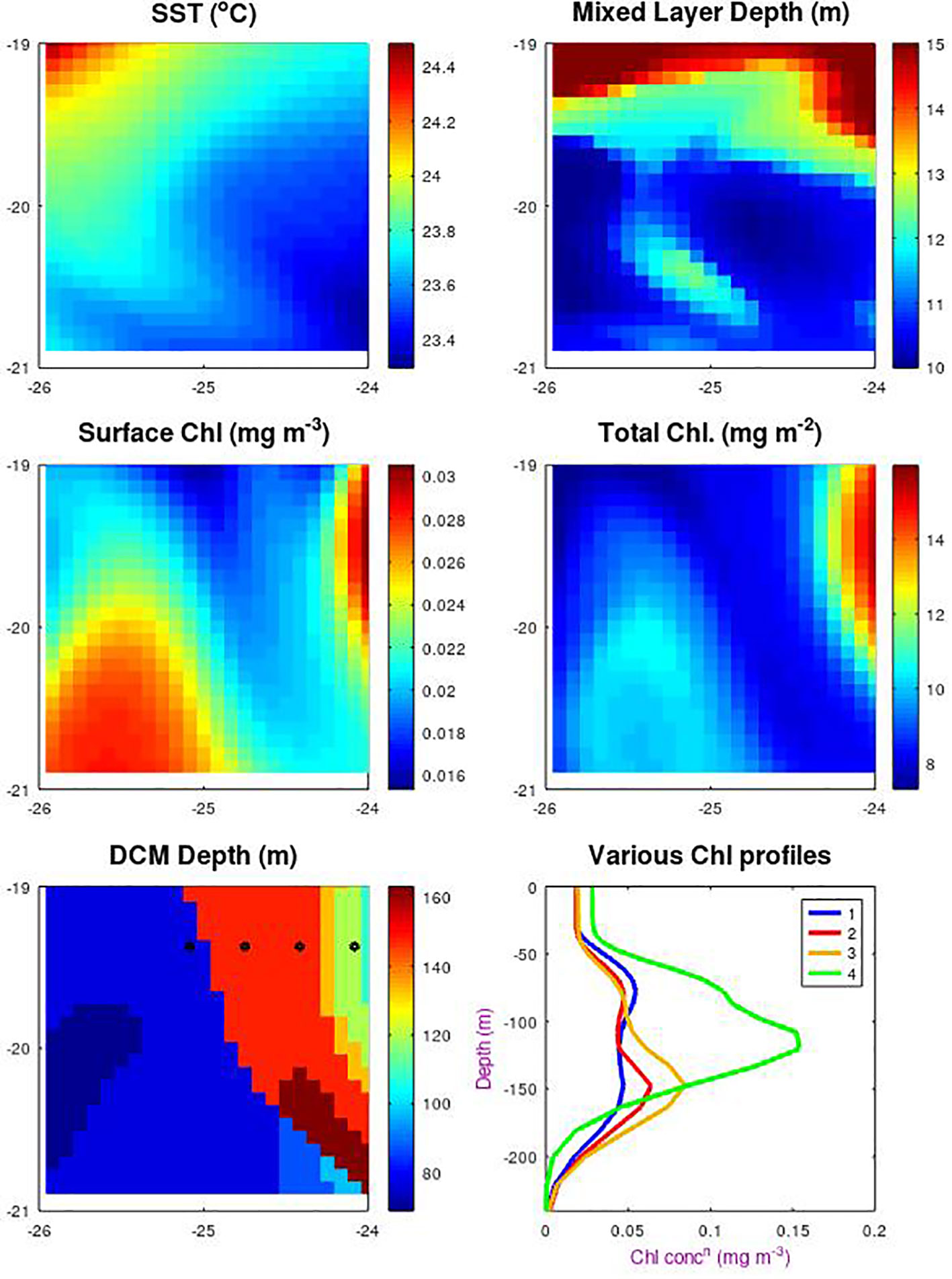
Figure A1 Spatial variations around SSTG within the MEDUSA model. Data are for a 2˚x2˚ square in Nov. 1998, with the top row showing sea surface temperature and mixed layer depth as indicators of the physical features present. Subsequent plots show the surface chlorophyll and the total column-integrated chlorophyll and the depth of the layer of maximum chlorophyll. The sixth plot shows the chlorophyll profiles at the 4 locations indicated by dots, showing how there can be a step change in the apparent DCM layer between the first two locations indicated by the blue and red profiles.
We also note that the definition of depth of DCM is inherently non-linear. The bottom two panels show the depth of the DCM and four of the vertical profiles. Moving gradually from west to east there is a point where the maximum ceases to be in the 80 m layer (as shown by the blue profile) and is now in the 150 m layer (shown in red). Although the line showing where 150 takes over from 80 m does align with the surface pattern, it would be hard to infer which depth was appropriate for the central point (the nominal location for all the other analyses). This indicates how hard it would be to predict the DCM depth at a point merely from surface observations.
Keywords: chlorophyll, subtropical gyre, Atlantic Meridional Transect, BGC-Argo, deep chlorophyll maximum, seasonal, interannual, model validation
Citation: Quartly GD, Aiken J, Brewin RJW and Yool A (2023) The link between surface and sub-surface chlorophyll-a in the centre of the Atlantic subtropical gyres: a comparison of observations and models. Front. Mar. Sci. 10:1197753. doi: 10.3389/fmars.2023.1197753
Received: 31 March 2023; Accepted: 06 November 2023;
Published: 29 November 2023.
Edited by:
Vanda Brotas, University of Lisbon, PortugalReviewed by:
Rajani Kanta Mishra, Ministry of Earth Sciences, IndiaJohn T. Bruun, University of Exeter, United Kingdom
Emmanuel Boss, University of Maine, United States
Copyright © 2023 Quartly, Aiken, Brewin and Yool. This is an open-access article distributed under the terms of the Creative Commons Attribution License (CC BY). The use, distribution or reproduction in other forums is permitted, provided the original author(s) and the copyright owner(s) are credited and that the original publication in this journal is cited, in accordance with accepted academic practice. No use, distribution or reproduction is permitted which does not comply with these terms.
*Correspondence: Graham D. Quartly, Z3F1QHBtbC5hYy51aw==