Assessment of austral autumn air–sea CO2 exchange in the Pacific sector of the Southern Ocean and dominant controlling factors

The factors that control the partial pressure of carbon dioxide (pCO₂) in the Pacific sector of the Southern Ocean were investigated in April 2018, onboard the icebreaker, ARAON. The mean (± 1σ) of the sea surface pCO₂ was estimated to be 431 ± 6 μatm in the north of the Ross Sea (NRS), 403 ± 18 μatm in the Amundsen–Bellingshausen Sea (ABS), and 426 ± 16 μatm in the western Antarctic Peninsula and Weddell Sea (WAP/WS). The controlling factors for pCO₂ in the NRS appeared to be meridionally different based on the southern boundary of the Antarctic Circumpolar Current (SB; ~62.5°S in the Ross Sea). The sea surface pCO₂ exhibited a strong correlation with salinity and the difference between the O₂/Ar (ΔO₂/Ar) values of the sample and air-saturated water in the north and south of the SB, respectively. The pCO₂ in the ABS and western WAP/WS displayed a strong correlation with salinity. Furthermore, ΔO₂/Ar and sea ice formation appear to be the dominant factors that control pCO₂ in the Confluence Zone (CZ) and northern parts of WAP/WS. The estimated air–sea CO₂ fluxes (positive and negative values indicate the source and sink for atmospheric CO₂, respectively) range from 3.1 to 18.8 mmol m⁻² d⁻¹ in the NRS, −12.7 to 17.3 mmol m⁻² d⁻¹ in the ABS, and −59.4 to 140.8 mmol m⁻² d⁻¹ in the WAP/WS. In addition, biology-driven large variations in the air–sea CO₂ flux were observed in the CZ. Our results are the most recent observation data acquired in austral autumn in the Southern Ocean.

Introduction

The Southern Ocean is known to strongly absorb atmospheric carbon dioxide (CO₂) because of the high CO₂ solubility, strong wind speed, and lower partial pressure of CO₂ (pCO₂) of its surface seawater. Although the Southern Ocean covers only 30% of the global ocean surface, it has absorbed more than 40% of anthropogenic CO₂ since the industrial revolution (Orr et al., 2001; Mikaloff Fletcher et al., 2006; Ito et al., 2010; DeVries, 2014). Horizontal and overturning circulations in the Southern Ocean form water masses with different physical and biogeochemical properties, which affect its CO₂ absorption capacity. The Antarctic Circumpolar Current (ACC) is a strong eastward-flowing current that encircles Antarctica. The Southern Ocean is divided into three regions based on the fronts associated with the ACC: (i) the Polar Frontal Zone (PFZ), which is located between the Subantarctic front (SAF) and the Polar front (PF); (ii) the Antarctic Southern Zone (ASZ), which is located between the PF and the southern boundary (SB) of the ACC; and (iii) the Seasonal Sea Ice Zone (SSIZ), which is located between the SB and Antarctica. Near the SB, the Circumpolar Deep Water (CDW) upwells via Ekman transport and diverges toward the SSIZ and PFZ (Speer et al., 2000; Ito et al., 2010). The CDW is elevated from the lower layer of the water column and has a high CO₂ content; therefore, CO₂ is released from the newly upwelled seawater to the atmosphere in this zone (Bushinsky et al., 2019). However, some studies suggested that CDW also increases the primary productivity because of its high nutrient concentrations and no prior exposure to anthropogenic CO₂, thereby, enhancing the absorption capacity of atmospheric CO₂ (Sokolov and Rintoul, 2007). An increase in the primary production in the ASZ may outweigh the outgassing of CO₂ caused by the upwelling of CO₂-rich waters. Direct field observations are necessary to confirm the effects of CDW.

The Southern Ocean is also divided into three regions based on longitude: (i) the Pacific sector, (ii) the Atlantic sector, and (iii) the Indian sector. Among them, the Pacific sector of the Southern Ocean includes the Ross Sea, Amundsen Sea, Bellingshausen Sea, and West Antarctic Peninsula (WAP) from west to east. The Ross Sea exhibits the largest phytoplankton bloom during spring and summer, which reduces surface pCO₂ and generates a strong atmospheric carbon sink (ranging from −4.7 to −15.6 mmol m⁻² d⁻¹, where negative values indicate air-to-sea flux) (Arrigo et al., 2008; DeJong and Dunbar, 2017). Similar to the Ross Sea, the Amundsen Sea is also a region with a high biological production (Arrigo et al., 2012). The oceanic pCO₂ in the Amundsen Sea exhibits a strong inverse relationship with biological activities, and the mean air–sea CO₂ flux is estimated to be −15.9 mmol m⁻² d⁻¹ during summer (Tortell et al., 2012). These two regions (i.e., Ross Sea and Amundsen Sea) form several polynyas during spring and summer. Polynyas have a substantially lower surface pCO₂ than pelagic pCO₂ because of their high biological production and low surface salinity (Tortell et al., 2012). Previous studies have suggested a relatively strong oceanic uptake of atmospheric CO₂ in the polynyas, ranging from −1.7 to −36.0 mmol m⁻² d⁻¹ in the Ross Sea and −36 to −41.9 mmol m⁻² d⁻¹ in the Amundsen Sea (Bates et al., 1998; Tortell et al., 2011; Tortell et al., 2012; Mu et al., 2014). The Bellingshausen Sea is a geographically important region that connects the WAP with the Amundsen Sea (Schulze Chretien et al., 2021). The mean air–sea CO₂ flux in the Bellingshausen Sea is estimated to be −1.5 mmol m⁻² d⁻¹, and it is characterized by a low surface pCO₂ (214–419 μatm) (Robertson and Watson, 1995; Ruiz-Halpern et al., 2014). However, significant seasonal CO₂ variations (ranging from −40 mmol m⁻² d⁻¹ during spring and summer to 40 mmol m⁻² d⁻¹ during autumn and winter) have been detected in the coastal areas of the region (i.e., Gerlache Strait) because of the changes in the surface CO₂-controlling factors due to upwelling during autumn and winter and biological activities during spring and summer (Monteiro et al., 2020).

As pronounced in the cases of the Ross Sea and Amundsen Sea, the influence of biological productivity on seawater pCO₂ during spring and summer is critical. In addition, this effect is connected to the dynamics of sea ice movement (i.e., formation of polynya). Considering that the majority of existing observational data predominantly targets seasons with elevated productivity, it is imperative to closely examine the substantial seasonal variability exhibited in the Bellingshausen Sea. As shown by Takahashi et al. (1993), oceanic pCO₂ exhibits a strong correlation with temperature. Temperature not only accounts for the thermodynamic variability of pCO₂, but also functions as an indicator of the intensity of vertical mixing (which generally accompanies an increase in pCO₂) along with salinity. Consequently, a thorough comprehension of the interplay between light availability, stratification resulting from seasonal sea ice formation and decline, organic carbon synthesis and decomposition by marine biota, as well as alterations in vertical mixing induced by wind, is essential for accurately discerning the air–sea CO₂ exchange dynamics in the Southern Ocean. Nonetheless, there is a significant lack of field surveys aimed at unraveling these factors affecting pCO₂ in the Southern Ocean.

There are several ways to observe the surface pCO₂ for calculation air–sea CO₂ flux, and most previous studies using ship-based observations have reported that the mean ocean uptake of atmospheric CO₂ ranges from –0.8 to 1.0 Pg C yr^–1 in the south of 50°S (McNeil et al., 2007; Takahashi et al., 2009) and –1.3 to –0.5 Pg C yr^–1 in the south of 35°S (Nevison et al., 2016). However, these estimations of the mean CO₂ uptake in the Southern Ocean are mostly based on data acquired during spring and summer. This is because the Southern Ocean has limited accessibility during autumn and winter because of harsh environmental conditions, such as high wind speeds and sea ice expansion. New profiling floats, deployed by the Southern Ocean Carbon and Climate Observations and Modeling project (hereafter SOCCOM floats), along with the development and deployment of uncrewed surface vehicles in the Southern Ocean have facilitated the acquisition of vertical profiles of a carbonate parameter (e.g., pH), independent of seasons (Sutton et al., 2021). A previous study reported that the inclusion or exclusion of observational data from colder seasons leads to significant differences in the air–sea CO₂ flux calculations (Bushinsky et al., 2019). Furthermore, Sutton et al. (2021) suggested that wind speed observation and sampling frequency are important factors for the estimation of air–sea CO₂ flux that can cause a significant bias in air–sea CO₂ flux, ranging from – 4% to +20% in the Southern Ocean. The application of such equipment could improve our understanding of the seasonal as well as interannual variabilities (i.e., Southern Annual Mode) in the carbon cycle in the Southern Ocean (Bushinsky et al., 2019). However, revealing spatial variations over large areas (while minimizing temporal variations) is only possible through shipboard underway measurements. Although the development of unmanned observation equipment (e.g., SOCCOM floats and uncrewed surface vehicles) and models (Lovenduski et al., 2015; Gregor et al., 2017) have improved our understanding of the carbon cycle in the Southern Ocean, these data need to be evaluated based on field data.

In this study, we measured the surface pCO₂ in the ASZ and SSIZ in the Pacific sector of the Southern Ocean in early autumn, and estimated the controlling factors that influence the variations in pCO₂ using our ship-based observations and SOCCOM float-based results. Our estimations are expected to aid in improving the understanding of the carbon cycle in autumn in the Southern Ocean, and the results can be utilized as fundamental data to reduce uncertainties in future studies.

Materials and methods

Field observations

This study was performed as part of the Antarctic Cruise program (ANA08D) of the Korea Polar Research Institute (KOPRI) in autumn from March 31, 2018 to April 27, 2018 using the icebreaker, ARAON, in the Pacific sector of the Southern Ocean (Figure 1). To compare the regional characteristics of the variations in surface pCO₂ and air–sea CO₂ flux in the Southern Ocean, the study area was divided into three regions, under the domains of the commission for the conservation of Antarctic marine living resources, as follows: the north of Ross Sea (NRS), Amundsen–Bellingshausen Sea (ABS), and WAP with Weddell Sea (WAP/WS) (Figure 1A). Our ship moved from northwest to southeast in the Pacific sector of the Southern Ocean. Thus, unlike the other two subregions, the NRS survey covered the meridional band between 60°S and 65°S and did not include areas that interact with the sea ice marginal zone of the Ross Sea. The WAP includes a Confluence Zone (CZ) between 67°W and 59°W, which is the transition zone between the Bellingshausen Sea and the Weddell Sea, and between the southern and northern parts of the WAP (S-WAP/WS and N-WAP/WS, respectively) (Figure 1B). In addition, two repeated cruises were conducted to survey between the Trinity peninsula and the King George Island in the Bransfield strait in order to evaluate the temporal variations in pCO₂. The first (BS1) and second (BS2) surveys in the Bransfield strait had a time interval of approximately two weeks (from April 11 to April 12 and from April 25 to April 26, respectively).

FIGURE 1

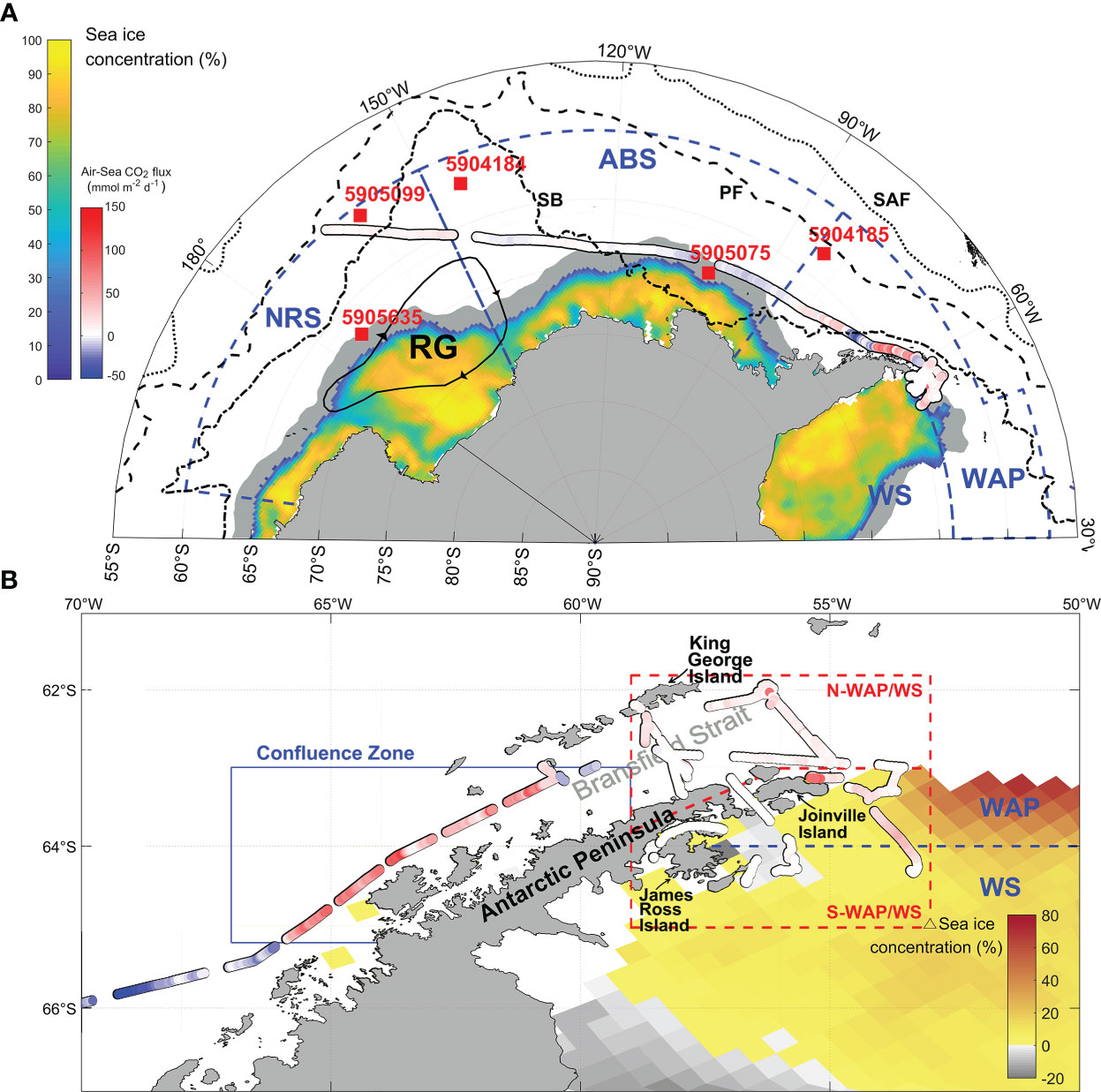
Figure 1 (A) Study regions in the Southern Ocean with sea ice concentrations determined on April 5, 2018 and the air–sea CO₂ flux (colors; positive and negative values meaning CO₂ source and sink, respectively). (B) Expanded map of the WAP and WS regions (WAP/WS) with changed sea ice concentrations between April 15 and April 30. Colors indicate the sampling date. The red squares in (A) indicate the position of the SOCCOM floats in April 2018. The dotted, dashed, and dash dotted lines represent the Subantarctic Front (SAF), Polar Front (PF), and Southern Boundary (SB) of Antarctic circumpolar current, respectively (Park and Durand, 2019). The colored lines in both figures represent the track of the IBRV ARAON. The blue dashed line in (A, B) represent the local boundaries. RS, AB, WAP, WS imply the Ross Sea, Amundsen–Bellingshausen Sea, Western Antarctic Peninsula, and Weddell Sea, respectively. The gray shading in (A) and the blue and red squares in (B) indicate the marginal sea ice zone, the Confluence Zone, and northern and southern WAP/WS, respectively.

During the cruise, the underway sea surface salinity (SSS) and temperature (SST) were measured using the SEB45 and SEB38 sensors, respectively. Further, data on wind speed were collected every 10 s using an automatic weather station installed at approximately 19 m above sea level. Additionally, the underway pCO₂ (${p\text{CO}}_2^{\text{sens}}$) was continuously determined during the ANA08D cruise using a carbon dioxide sensor (CONTROS HydroC CO₂, Germany). This sensor uses optical non-dispersive infrared gas detection to measure the oceanic pCO₂ in different environments (Fietzek et al., 2014; Marrec et al., 2014; Totland et al., 2020; Macovei et al., 2021). Zeroing was conducted every 6 h to adjust the drifting of the baseline during the observation. An equilibrator-type commercial underway pCO₂ system (GO system; General Oceanics, USA) was also installed in the ARAON. However, the equilibrator-based pCO₂ data, for comparison with ${p\text{CO}}_2^{\text{sens}}$, could not be acquired due to an unexpected system malfunction. Instead, surface seawater samples were collected every day during the cruise to calibrate ${p\text{CO}}_2^{\text{sens}}$obtained from the sensor (Marrec et al., 2014). The seawater samples were collected into 500 mL borosilicate bottles and immediately mixed with 200 μL of saturated mercury (II) chloride (HgCl₂) solution to inhibit biological activities. The mixed solution was stored at room temperature until the analysis. The total alkalinity (TA) and dissolved inorganic carbon (DIC) were measured using Versatile Instrument for the Determination of Titration Alkalinity 3C (VINDTA 3C, Germany). Routine analyses performed using certified reference materials (obtained from Prof. A. Dickson, Scripps Institute of Oceanography (USA)) ensured that the analytical precisions for the TA and DIC measurements were approximately 2 and 1 μmol kg⁻¹, respectively. The CO2SYS program developed by Lewis and Wallace (1998) was used to calculate pCO₂ (${p\text{CO}}_2^{\text{calc}}$) from the measured SSS, SST, TA, and DIC using the carbonate dissociation constants provided by Mehrbach et al. (1973) refitted by Dickson and Millero (1987) and the ancillary thermodynamic constants reported by Millero (1995). We averaged the ${p\text{CO}}_2^{\text{sens}}$data collected for 20 min before and after collecting the surface seawater samples for the determination of TA and DIC. The resulting mean ${p\text{CO}}_2^{\text{sens}}$values were directly compared with the ${p\text{CO}}_2^{\text{calc}}$values calculated from the corresponding TA and DIC values, and a robust linear fit between ${p\text{CO}}_2^{\text{sens}}$and ${p\text{CO}}_2^{\text{calc}}$was observed (Figure S1A). The regression equation was applied to the 10-min mean ${p\text{CO}}_2^{\text{sens}}$values to obtain the pCO₂ data (${p\text{CO}}_2^{\text{obs}}$) used in this study (Figure S1B). Before this calibration procedure, the ${p\text{CO}}_2^{\text{sens}}$values were corrected for the difference between in situ SST and shipboard laboratory temperature. The ${p\text{CO}}_2^{\text{calc}}$was calculated using in situ SST. As indicated, the ${p\text{CO}}_2^{\text{sens}}$-based ${p\text{CO}}_2^{\text{obs}}$data were used in this study because of malfunction of the high-precision GO system, which may affect the quality of the individual pCO₂ values. However, on a regional scale, we believe that the mean ${p\text{CO}}_2^{\text{obs}}$values can represent the overall regional conditions owing to the data calibration based on the bottle data. In addition, our data were sufficient to examine the spatiotemporal variations (i.e., relative changes) in pCO₂, because ${p\text{CO}}_2^{\text{obs}}$showed significant correlations with the related variables (see discussion).

The underway analysis of the gas ratios between oxygen and argon (O₂/Ar) were performed using a membrane inlet mass spectrometer (Hiden Analytical, UK) to estimate the degree of oxygen supersaturation by biological activities (see below). Kim et al. (2017) presented a more detailed measurement method for O₂/Ar. Finally, the difference between the O₂/Ar (ΔO₂/Ar) values of the sample and air-saturated water was used to isolate the O₂ produced by the biological activities.

$\begin{array}{ll}\text{Δ}{\text{O}}_2/{\text{Ar = (O}}_2/{\text{Ar)}}^{\text{sample}}/{{\text{(O}}_2/\text{Ar)}}^{\text{sat}}-1,& \text{(Eq. 1)}\end{array}$

where the superscripts “sample” and “sat” represent the O₂/Ar values in the sample and air-saturated water, respectively. The O₂/Ar can be altered by biological activities (e.g., photosynthesis and respiration) and physical processes (e.g., mixing of water masses) (Eveleth et al., 2014).

Data from the SOCCOM floats

In addition to the field survey data, we used the data obtained from the SOCCOM floats (data available in soccom.princeton.edu/content/data-access). Five floats (5904184, 5904185, 5905075, 5905099, and 5905635) were found over our study area and period. Their pCO₂ (with an accuracy of ±11 μatm; Williams et al., 2018) and DIC (with an accuracy of ±4 μatm; Williams et al., 2018) values were derived from in situ pH sensor (with an accuracy of ±0.01; Johnson et al., 2016) in the floats and algorithm-based predicted TA (with an accuracy of ±5.4 μmol kg⁻¹; Carter et al., 2017). The determined SOCCOM pCO₂ values were compared with our ship-based pCO₂ data to evaluate their consistency. Additionally, we utilized SOCCOM float data to evaluate the effects of temporal variations in environmental variables such as SSS, SST, TA, and DIC on pCO₂ values. To maintain consistency with our field survey period, we used data collected in April 2018. To understand the overall changes occurring during the given month, we incorporated the first and last data recorded in April into our calculations. Following the approach proposed by Williams et al. (2018), and using the CO2SYS software (Lewis and Wallace, 1998) in conjunction with elemental stoichiometric relationships, we were able to investigate the influence of monthly shifts in each variable on pCO₂ during April.

Calculation of thermal versus non-thermal pCO₂

The effect of temperature variation (i.e., thermal effect) on pCO₂ can be distinguished from the effects of other environmental factors (i.e., non-thermal effects; mainly physical mixing and biology). pCO₂ (4.23% °C^–1, Takahashi et al., 2002) values vary in response to changes in temperature, which originate from the temperature dependence of the gas solubility of CO₂ as well as the dissociation constants of the dissolved inorganic carbon species. However, non-thermal effects include alternations in TA and DIC caused by the physical mixing of water masses and biological activities (e.g., organic matter formation and degradation). The thermal and non-thermal effects on the variations in pCO₂ can be derived using the following equations (Takahashi et al., 2002):

$\begin{array}{ll}{p\text{CO}}_2^{\text{th}}{\text{ = }p\text{CO}}_2^{\text{mean}}{\times \text{e}}^{\mathrm{[0}{.0423\times \text{(SST}}^{\text{obs}}-{\text{SST}}^{\text{mean}}\text{)]}},& \text{(Eq. 2)}\end{array}$

$\begin{array}{ll}{p\text{CO}}_2^{nt}{\text{ = }p\text{CO}}_2^{\text{obs}}{\times \text{e}}^{\mathrm{[0}{.0423\times \text{(SST}}^{\text{mean}}-{\text{SST}}^{\text{obs}}\text{)]}},& \text{(Eq. 3)}\end{array}$

where ${p\text{CO}}_2^{\text{th}}$and ${p\text{CO}}_2^{\text{nt}}$indicate the thermal and non-thermal pCO₂ components, respectively; the superscript “obs” represents the observed individual data; the subscript “mean” indicates a mean value for the study period; ${p\text{CO}}_2^{\text{mean}}$and SST^mean were 424 μatm and 1.1°C during our field survey period, respectively, and 395 μatm and 0.7°C in the SOCCOM data, respectively. In the data analysis elucidated below, the 10-min averaged values have been used for ${p\text{CO}}_2^{\text{obs}}$and ${\text{SST}}^{\text{obs}}$. Separation of the contributions of the thermal and non-thermal effects in pCO₂ is generally applied to determine the dominant factors that affect the seasonal pCO₂ variations in a fixed location (e.g., Takahashi et al., 2002; Ko et al., 2022). However, in this study, this method was primarily used to correct for thermal effects associated with spatial variations in SST.

Calculation of the air–sea CO₂ flux

The following parameters were used to calculate air–sea CO₂ flux $: {p\text{CO}}_2^{\text{obs}}$, SSS, SST, atmospheric pCO₂ (${p\text{CO}}_2^{\text{air}})$and the shipboard wind speed, which was adjusted for a height of 10 m (U₁₀) following the study of Thomas et al. (2005). Because wind speed could not be measured directly at the SOCCOM float locations, the mean wind speed observed during the cruise (approximately 11.9 m s^–1) was used for the floats. ${p\text{CO}}_2^{\text{air}}$was obtained from the US Palmer station located on the Anvers Island in WAP, and the monthly mean ${p\text{CO}}_2^{\text{air}}$was approximately 404 μatm in April 2018 (Dlugokencky et al., 2021; available at https://www.esrl.noaa.gov/gmd/dv/data/).

The following equation was used to calculate the air–sea CO₂ flux (in mmol m⁻² d⁻¹):

$\begin{array}{ll}{\text{air–sea CO}}_2{\text{ flux}=k\times s\times (p\text{CO}}_2^{\text{obs}}-404),& \text{(Eq. 4)}\end{array}$

where s is the solubility of CO₂ in seawater (mol L⁻¹ atm⁻¹) and is a function of salinity and temperature (Weiss, 1974); k is the CO₂ gas transfer velocity (cm h⁻¹), which was calculated using the following equation (Wanninkhof, 2014):

$\begin{array}{ll}\mathrm{k = 0}{.251\times \text{U}}_{10}^2\times {(\text{Sc}/660)}^{-0.5},& \text{(Eq. 5)}\end{array}$

where 0.251 (cm h⁻¹) (m s⁻¹) ⁻² is the optimal coefficient of CO₂ gas transfer, and Sc is the Schmidt number reported by Wanninkhof (2014).

Sea ice distribution

The daily polar gridded sea ice concentration obtained from the near-real-time Defense Meteorological Satellite Program with the Special Sensors Microwave Imager/Sounder daily polar gridded sea ice concentration on April 5, 2018 was used to distinguish the marginal sea ice zone during the cruise (data available in https://nsidc.org/data/NSIDC-0081/versions/1; Figure 1A) (Maslanik and Stroeve, 1999) as well as the changes in the sea ice concentration between April 15 and April 30 in the N-WAP/WS region (Figure 1B). Further, the marginal sea ice zone was estimated to be up to 200 km from the edge of the ice (Wadhams, 1986).

Results

Hydrological properties

The overall SST in the Pacific sector of the Southern Ocean ranged from −0.7 to 3.7 °C during the period of our study (Figure S2). The mean ( ± 1σ) values of the SST in the NRS, ABS, and WAP/WS were 1.9 ± 0.7 °C, 0.8 ± 0.2 °C, and 1.0 ± 1.1 °C, respectively. A relatively low SST was found near the marginal sea ice zone in the ABS and WAP/WS. The lowest SST, ranging from −0.7 to 2.8°C, was observed in the WAP/WS. The mean SST in the western part of the CZ (2.0 ± 0.4 °C) was higher than that in the N-WAP/WS (1.5 ± 1.0 °C). The SST in the CZ ranged from 1.0 to 2.5 °C and showed the greatest variability during short observation durations (1.9 days). In particular, the SST differed significantly between the N-WAP/WS and S-WAP/WS. The SST in the N-WAP/WS was clearly higher than that in the S-WAP/WS (0.0 ± 0.4 °C). Finally, significant changes in the SST were observed during the repeated observations in the Bransfield strait (i.e., between the Trinity peninsula and the King George Island). The mean SST values were 1.1 ± 0.8 °C and 1.3 ± 0.5 °C during the BS1 (from April 11 to April 12) and BS2 (from April 25 to April 26) observations, respectively.

During the study, the SSS ranged from 33.06 to 34.25 psu (Figure S2). The mean SSS values in the NRS, ABS, and WAP/WS were 33.56 ± 0.09 psu, 33.24 ± 0.08 psu, and 33.71 ± 0.25 psu, respectively. The SSS in the ABS and the western part of the CZ were relatively lower than that in the other regions. In the CZ, the SSS rapidly increased from 33.28 to 33.73 psu. The SSS difference between N-WAP/WS (33.81 ± 0.14 psu) and S-WAP/WS (33.86 ± 0.17 psu) was smaller than the temporal variations observed between the BS1 and BS2 surveys (33.62 ± 0.04 and 33.93 ± 0.06 psu, respectively).

Two SOCCOM floats (No. 5904184 and 5905635) were in the south of the SB, while the other floats were between the PF and SB (Figure 1A). The SST recorded by the SOCCOM floats showed a decreasing trend during April (Table S1). The SST near the marginal sea ice zone in the Ross Sea (float No. 5905635) and ABS (float No. 5905075) showed subzero temperatures during April. However, the SSS recorded by the SOCCOM floats showed a small variation during April, indicating a mean ( ± 1σ) SSS of 33.9 ± 0.1 psu.

Distribution of pCO₂

The overall ${p\text{CO}}_2^{\text{obs}}$(i.e., 10-min average of ${p\text{CO}}_2^{\text{sens}}$) ranged from 366 to 467 μatm in our study (Figures 2A–C). The mean ${p\text{CO}}_2^{\text{obs}}$values were 431 ± 6, 403 ± 18, and 429 ± 16 μatm in the NRS, ABS, and WAP/WS, respectively. In particular, ${p\text{CO}}_2^{\text{obs}}$in the western part of the WAP (i.e., from 85°W to 60°W) displayed a high variability, ranging from 375 to 430 μatm in the western part of the CZ and 384 to 467 μatm in the CZ. Observed ${p\text{CO}}_2^{\text{obs}}$values showed a similar range in the Bransfield Strait for two weeks. The ${p\text{CO}}_2^{\text{obs}}$values ranged from 403 to 454 μatm and from 406 to 461 μatm during the BS1 and BS2 observations, respectively. The spatiotemporal variations in the SST significantly affected the sea surface pCO₂. Accordingly, we separated ${p\text{CO}}_2^{\text{th}}$and ${p\text{CO}}_2^{\text{nt}}$for describing the pCO₂ variations in the subregions investigated in this study.

FIGURE 2

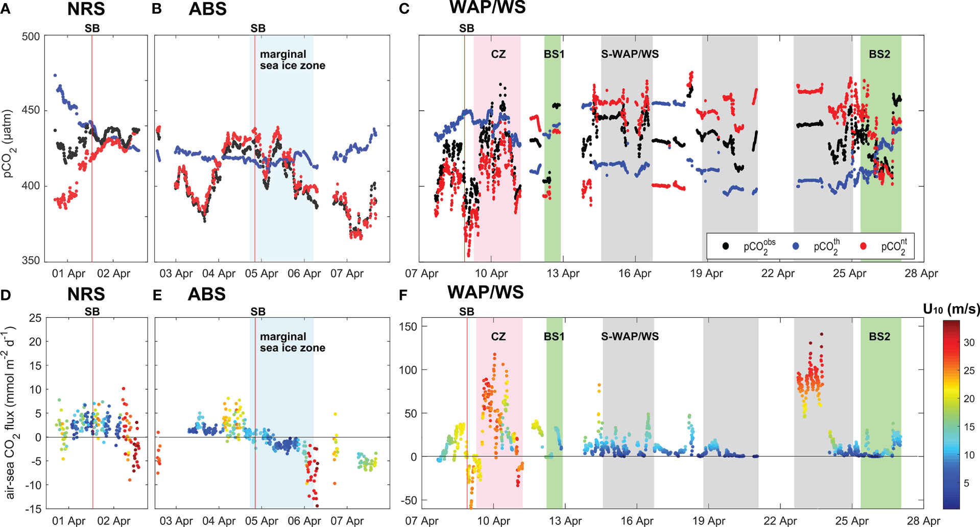
Figure 2 (A–C) Observed pCO₂ (${p\text{CO}}_2^{\text{obs}}$; black), thermal pCO₂ (${p\text{CO}}_2^{\text{th}}$; blue), and non-thermal pCO₂ (${p\text{CO}}_2^{\text{nt}}$; red) distribution. (D–F) Distribution of the air–sea CO₂ flux and wind speed (U₁₀; colors) in the north of Ross Sea (NRS), the Amundsen-Bellingshausen Sea (ABS), and the Western Antarctic Peninsula with the Weddell Sea (WAP/WS). The blue and pink shadings indicate the result in the marginal sea ice zone and Confluence Zone (CZ), respectively. The green shadings show the observations taken twice at different time periods in the Bransfield Strait. And the gray shadings represent the result in the south of WAP/WS (S-WAP/WS). Finally, the red vertical lines indicate the Southern boundary of the Antarctic Circumpolar Current (SB).

The ${p\text{CO}}_2^{\text{th}}$data, in which the effects of nonthermal factors (e.g., SSS, TA, DIC) were removed, gradually decreased from 473 to 424 μatm in the NRS (Figure 2A). Although ${p\text{CO}}_2^{\text{th}}$exhibited small variations in the ABS (420 ± 4 μatm), ${p\text{CO}}_2^{\text{th}}$was found to be reduced in the seawater around sea ice (i.e., from April 4 to April 6 in Figure 1A). Finally, the ${p\text{CO}}_2^{\text{th}}$in the WAP/WS showed very large variability in time and space (Figure 2C). The mean ${p\text{CO}}_2^{\text{th}}$was 406 ± 7 μatm in the S-WAP/WS, and 424 ± 14 μatm and 428 ± 9 μatm during the BS1 and BS2 observations, respectively. Obviously, those changes in ${p\text{CO}}_2^{\text{th}}$were the effect of SST variations.

The ${p\text{CO}}_2^{\text{nt}}$data, in which thermal effects were removed, gradually increased in the NRS, ranging from 386 to 437 μatm (Figure 2A). The distribution of ${p\text{CO}}_2^{\text{nt}}$was similar to that of ${p\text{CO}}_2^{\text{obs}}$in the ABS, entrance of the WAP/WS, and CZ because of the small SST variation in these areas (Figures 2A–C). The ${p\text{CO}}_2^{\text{nt}}$value ranged from 365 to 439 μatm in the ABS, 354 to 418 μatm in the western part of the CZ, and 368 to 442 μatm in the CZ. In addition, the distribution of ${p\text{CO}}_2^{\text{nt}}$in the northern tip of the Antarctic peninsula (i.e., N-WAP/WS and S-WAP/WS) showed a high spatiotemporal variation, although it was opposite to the ${p\text{CO}}_2^{\text{th}}$distribution (Figure 2C). The ${p\text{CO}}_2^{\text{nt}}$value ranged from 388 to 475 μatm in the N-WAP/WS and from 433 to 472 μatm in the S-WAP/WS. In general, changes in ${p\text{CO}}_2^{\text{nt}}$are mainly associated with biological carbon fixation and vertical mixing reducing and enhancing pCO₂, respectively.

Considering the five SCCCOM floats, pCO₂ ranged from 358 to 421 μatm during April (Table S1). A relatively low pCO₂ was found in the floats located near the sea ice (i.e., float No. 5905075 and 5905635). In general, pCO₂ increased with time during April, except for the float in the WAP (i.e., float No. 5904185). Float No. 5905635 showed the broadest pCO₂ range from 358 to 386 μatm. ${p\text{CO}}_2^{\text{th}}$gradually decreased from 433 to 360 μatm with time during April because of the decreasing SST. In contrast, ${p\text{CO}}_2^{\text{nt}}$generally increased from 373 to 420 μatm, except for the float No. 5904185.

Air–sea CO₂ flux

The overall air–sea CO₂ flux in the study area ranged from −59.4 to 140.8 mmol m⁻² d⁻¹ during the cruise (Figures 2D–F). The air–sea CO₂ flux in the NRS and ABS ranged from 3.1 to 18.8 mmol m⁻² d⁻¹ and −12.7 to 17.3 mmol m⁻² d⁻¹, respectively. The air–sea CO₂ flux in the WAP/WS ranged from −59.4 to 140.8 mmol m⁻² d⁻¹; however, it showed a high spatial variability depending on the local environmental condition. The air–sea CO₂ flux in the CZ, N-WAP/WS, and S-WAP/WS ranged from −33.4 to 117.6 mmol m⁻² d⁻¹, 0.0 to 82.4 mmol m⁻² d⁻¹, and 0.0 to 140.8 mmol m⁻² d⁻¹, respectively. Finally, a significant change in the air–sea CO₂ flux was observed in the Bransfield strait, with a mean of 21.3 ± 14.9 mmol m⁻² d⁻¹ and 8.4 ± 9.2 mmol m⁻² d⁻¹ during the BS1 and BS2 observations, respectively.

The air–sea CO₂ flux of the five SOCCOM floats ranged from −13.9 to 5.0 mmol m⁻² d⁻¹ during April (Table S1). Notably, two floats adjacent to sea ice exhibited a significant uptake of atmospheric CO₂. The mean air–sea CO₂ fluxes for these floats were −12.6 ± 1.2 mmol m⁻² d⁻¹ and −8.3 ± 4.9 mmol m⁻² d⁻¹ for floats NO. 5905075 and No. 5905635, respectively. In contrast, the other three floats showed a weak efflux of CO₂ to the atmosphere. The mean values for these floats were 2.0 ± 0.5 mmol m⁻² d⁻¹, 0.7 ± 1.3 mmol m⁻² d⁻¹, and 3.9 ± 1.2 mmol m⁻² d⁻¹ for float No. 590418, 5904185, and 5905099, respectively.

ΔO₂/Ar

During the cruise, the ΔO₂/Ar in the study area ranged from −1.8 to 4.9% (Figure S3). The mean ΔO₂/Ar values in the NRS and ABS were 0.9 ± 1.2 and −0.3 ± 2.3%, respectively, whereas that the WAP/WS was −3.7 ± 1.9%. The highest ΔO₂/Ar (4.9%) was observed in the western part of the CZ, while the lowest ΔO₂/Ar (−9.5%) was shown in the northern tip of the Antarctic peninsula. The ΔO₂/Ar in the CZ ranged from −8.8 to 4.9%, and the ΔO₂/Ar in the N-WAP/WS (−2.8 ± 1.6%) was higher than those in the S-WAP/WS (−4.2 ± 1.9%). In the Bransfield strait, the mean ΔO₂/Ar during the BS1 observation (−2.0 ± 0.7%) was relatively higher than that during the BS2 observation (−3.0 ± 2.0%).

Discussion

Comparison between the SOCCOM float and underway pCO₂ values

To assess the consistency between the shipboard underway and SOCCOM float pCO₂ data, which has an 11 μatm of uncertainty at 400 μatm (Williams et al., 2017), two SOCCOM floats (No. 5905099 and 5905075) were selected because of their proximity with our cruise track. Nonetheless, the distances from our cruise track to the two floats were ~145 km (No. 5905099) and ~60 km (No. 5905075) (Table 1). In addition, there was a 3-day difference in the observation date between the shipboard and float pCO₂ data. The pCO₂ differences between the two platforms were ~19 μatm (No. 5905099) and ~33 μatm (No. 5905075). In the case of the 5905075 float, the pCO₂ difference reduced to ~4 μatm if the effect of the SST difference was corrected (i.e., ${p\text{CO}}_2^{\text{nt}}$was compared). In contrast, for the No. 5905099 float, there was still a difference of 20 μatm even after the temperature correction was applied. This discrepancy may be attributed to the considerable distance (~145 km) between the two platforms. Fay et al. (2018) also conducted a comparison between shipboard pCO₂ data and data collected within three days from SOCCOM floats located within a 75 km radius of their ship’s track. Their findings also indicated a similar difference (~ 24 μatm) to those observed in this study, which ranged between 19 and 33 μatm.

TABLE 1

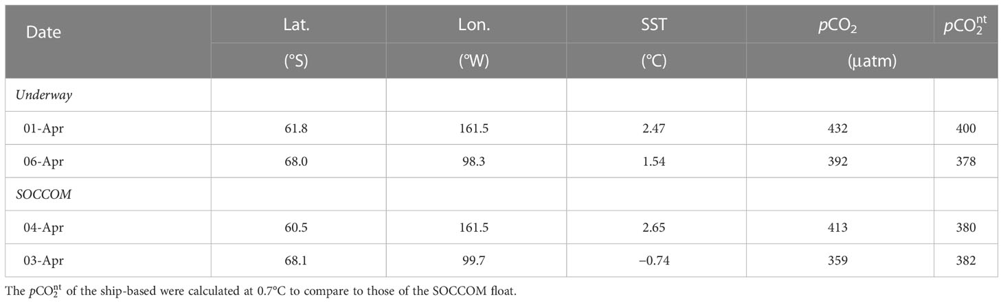
Table 1 Latitude (Lat.) and longitude (Lon.), sea surface temperature (SST), underway pCO₂, and non-thermal pCO₂ ( ${p\text{CO}}_2^{\text{nt}}$) data for comparison between the ship-based and SOCCOM float-based observation results.

Quantifying environmental factors influencing pCO₂ of SOCCOM floats

To identify the factors that control pCO₂ in the study area, we determined the influence of each factor (e.g., SST, SSS, TA, and DIC) using CO2SYS and SOCCOM float pCO₂ data (Table 2). CO₂ solubility in seawater is a function of salinity, temperature, and pressure (Weiss, 1974). Under a constant pressure (surface), a decrease in salinity and temperature can enhance the CO₂ solubility. The SST-driven change in pCO₂ ($\Delta {p\text{CO}}_2^{\Delta \text{SST}}$= [pCO₂ at the last observation in April] – [pCO₂ at the first observation in April]) ranged from −12.7 to −6.5 μatm in the study area because of the decreasing SST in April. However, the SSS-driven changes ($\Delta {p\text{CO}}_2^{\Delta \text{SSS}}$) were much smaller ($\Delta {p\text{CO}}_2^{\Delta \text{SSS}}$= ± 0.4 μatm) because of the relatively low variations in the SSS ($\Delta \text{SSS=}$~0.05). The changes in pCO₂ ($\Delta {p\text{CO}}_2^{\Delta \text{TA}}$) associated with TA ranged from −12.6 to 7.6 μatm, while those in pCO₂ ($\Delta {p\text{CO}}_2^{\Delta \text{DIC}}$) associated with DIC ranged from 5.9 to 30.5 μatm in April 2018. Finally, residual in pCO₂ ($\Delta {p\text{CO}}_2^{\Delta \text{RESID}}$) showed a variation from 0.0 to 2.3 μatm after the removal of the $\Delta {p\text{CO}}_2^{\Delta \text{SST}}$, $\Delta {p\text{CO}}_2^{\Delta \text{SSS}}$, $\Delta {p\text{CO}}_2^{\Delta \text{TA}}$, and $\Delta {p\text{CO}}_2^{\Delta \text{DIC}}$effects. These results suggest that the effects of the SST, TA, and DIC are significant in all the floats; however, the SSS exudes the least impact on pCO₂ due to small variation of SSS in April 2018.

TABLE 2

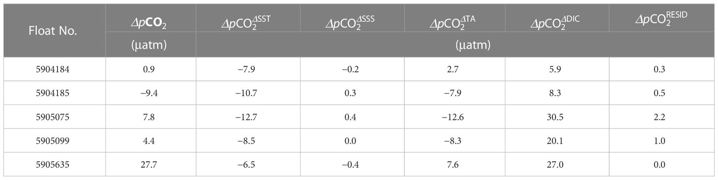
Table 2 Contributions of various factors in the pCO₂ variations observed in the SOCCOM floats.

ΔTA and ΔDIC (estimated from SOCCOM data) were decomposed to understand the processes causing their variations, such as freshwater input, organic matter, calcium carbonate (CaCO₃), and gas exchange, using a formula reported by Williams et al. (2018) (Table 3). In their approach, the SSS, nitrate $({\text{NO}}_3^{-})$ , DIC : TA ratio were used to separate the effect of freshwater, organic matter decomposition/synthesis, and calcification. Because the suggested method requires nitrate $({\text{NO}}_3^{-})$ concentration, we could use three floats except for the 5904184 and 5904185 floats, in which $({\text{NO}}_3^{-})$ concentrations were not available. The analysis suggested that freshwater and CaCO₃ dissolution were the dominant factors for ΔTA. In contrast, the variations in DIC were not associated with the freshwater input, biological activities, and gas exchanges, and thus, the largest values of the residual term were obtained in this case. Since we did not measure the wind speed directly at the SOCCOM float locations, the gas exchange term could not be accurately determined. The gas exchange term did not affect other terms accompanying the changes in TA. Williams et al. (2018) studied the eastern Antarctic Ocean region and suggested that freshwater input and CaCO₃ dissolution/formation govern the TA variations in the ASZ (i.e., between PF and SB), while the TA in the SSIZ is substantially influenced by the freshwater input (i.e., south of SB). In addition, they suggested that organic matter production/remineralization is the most dominant factor that influences the changes in DIC, followed by the freshwater input. Our results for TA were consistent with those of the previous study, whereas those of DIC were not identical.

TABLE 3

Table 3 Contribution of each factor on total alkalinity (TA) and dissolved inorganic carbon (DIC).

Ross sea sector

The ${p\text{CO}}_2^{\text{obs}}$and ${p\text{CO}}_2^{\text{nt}}$values in the NRS increased as the icebreaker moved southeast through the PF and SB, while the ${p\text{CO}}_2^{\text{th}}$in this region decreased during the cruise (Figures 1A, 2A), indicating that the non-thermal factors control the ${p\text{CO}}_2^{\text{obs}}$variations in the NRS. According to a previous study, ${p\text{CO}}_2^{\text{obs}}$between the PF and SB ranged from 331 to 354 μatm in December 2005 (Guéguen and Tortell, 2008). Even considering the atmospheric CO₂ growth from 378 to 404 μatm, the value observed in summer was lower than those shown in our autumn survey. The relatively high ${p\text{CO}}_2^{\text{obs}}$in this study might have resulted from the increase in the mixed layer depth (MLD) due to strong winds and the remineralization of the organic matter produced in summer. The mean U₁₀ in the NRS was 9.9 ± 1.5 m s⁻¹, and ranged from 7.7 m s⁻¹ to 13.0 m s⁻¹ in April, which was relatively greater than that in summer (ranging from 4.0 to 7.9 m s⁻¹) (Guéguen and Tortell, 2008; DeJong and Dunbar, 2017). Along the survey track, the surface water in the SB (62.5°S) was the most saline and had a relatively high temperature, indicating an influence from the upwelling of or enhanced mixing with the sub-surface water, which is relatively rich in CO₂ and nutrients (Figure S2A). In addition, a correlation analysis indicated that the main controlling factors of ${p\text{CO}}_2^{\text{nt}}$were SSS (e.g., physical effects such as changes in mixing and sea ice) and ΔO₂/Ar (i.e., biological effects) in the north and south of the SB, respectively (Figure 3). Guéguen and Tortell (2008) found no significant correlation between pCO₂ and the SSS over the ocean from New Zealand to the Ross Sea during summer. Thus, the significant correlation between SSS and ${p\text{CO}}_2^{\text{nt}}$was a local characteristic limited to the 62.5 to 65°S zone or April (autumn). It is well known that CDW upwelling occurs near the SB, and the upwelled CDW diverges from the SB to the PF and to the Antarctic shelf region (Speer et al., 2000). At the SB, high biological activities are found because of the upwelling of the nutrient-rich subsurface water (Sokolov and Rintoul, 2007). In addition, Rigual-Hernández et al. (2015) reported a relatively high concentration of chlorophyll-a in the Southern ACC Front (SACCF, located in ASZ) in the Antarctic coastal area, while low chlorophyll-a concentrations were found from the SACCF to New Zealand. Therefore, ${p\text{CO}}_2^{\text{nt}}$in seawater, which was transferred from the SB to coastal areas, might have been altered by biological activities. ${p\text{CO}}_2^{\text{nt}}$decreases because of the net biological CO₂ uptake (i.e., ΔO₂/Ar > 0) when the phytoplankton production surpasses the ecosystem respiration. In contrast, ${p\text{CO}}_2^{\text{nt}}$increases when ΔO₂/Ar< 0. Accordingly, it was likely that ${p\text{CO}}_2^{\text{nt}}$was largely controlled by the upwelling at the SB and the following biological activities in the NRS in April 2018. Our data clearly highlighted a shift in the ecosystem dynamics associated with the inorganic carbon cycle across the SB.

FIGURE 3

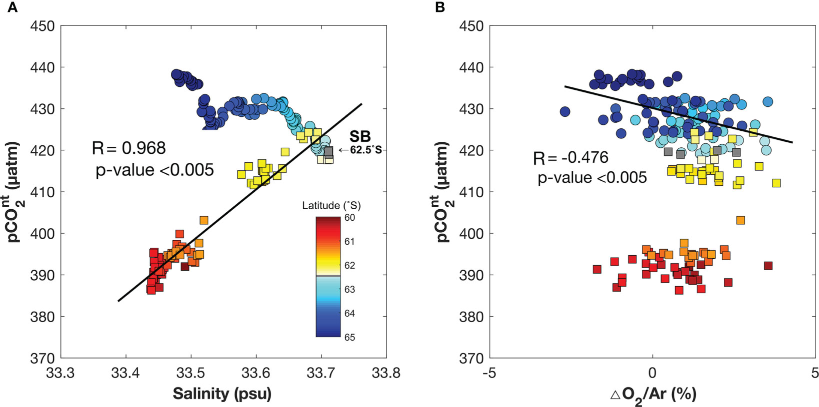
Figure 3 Relationship between the nonthermal component of pCO₂ (${p\text{CO}}_2^{\text{nt}}$) and (A) salinity and (B) the difference in the gas ratios between oxygen and argon O₂/Ar values of the sample and air-saturated water (ΔO₂/Ar) (B) in the north of the Ross Sea. The north of the Ross Sea is further divided into northern (i.e.,<62.5°S) (squares) and southern (i.e., >62.5°S) parts (circles) based on the Southern Boundary (SB) of the Antarctic circumpolar current. The colored legends represent the latitude, and the gray color implies the latitude of the SB. The regression lines in (A, B) are determined using the northern and southern part results, respectively.

The NRS acted as an overall CO₂ source (8.8 ± 3.5 mmol m⁻² d⁻¹) for atmospheric CO₂ during April. The amount of CO₂ released from the ocean to the atmosphere was increased in the eastern part of the NRS, which had a relatively higher ${p\text{CO}}_2^{\text{obs}}$(than ABS), high wind speeds, and a heterotrophic ecosystem (i.e., negative ΔO₂/Ar) in the observation period (Figures 2A, C and S3A). The NRS and the Ross Sea exhibited different patterns with respect to air–sea exchange of CO₂. Most previous studies on air–sea CO₂ flux were conducted during spring and summer in the southwestern Ross Sea, and suggest that the air–sea CO₂ flux ranges from −132 to 10 mmol m⁻² d⁻¹ (Arrigo and Van Dijken, 2007; DeJong and Dunbar, 2017). Thus, Ross Sea has been considered to act as a CO₂ sink during spring and summer because of the enhanced biological activities (DeJong et al., 2017; Rivaro et al., 2017). In particular, the Terra Nova Bay in the Ross Sea acts as a strong sink for atmospheric CO₂ (up to −132 mmol m⁻² d⁻¹) (DeJong and Dunbar, 2017). The discrepancies between the findings in the NRS and the previous research results from the Ross Sea can likely be attributed to the differences in productivity between the two regions and the variations in the timing of the respective investigations. In general, the rate of photosynthesis by the phytoplankton increases from spring to summer because of the abundance of sunlight and nutrients due to the shrinking of the sea ice (Zhang et al., 2010; Hill et al., 2018; Lannuzel et al., 2020). This effect can help elucidate the strong CO₂ sink observed in studies conducted in the Ross Sea, where most previous research is primarily focused during the summer. In autumn, pCO₂ likely increases due to enhanced vertical mixing and the decomposition of organic matter that has accumulated from biological activities in previous seasons. These factors are likely to outweigh CO₂ fixation in the pelagic water (i.e., NRS) with relatively lower nutrient concentrations, especially during autumn when light availability is reduced. In addition, a relatively high pCO₂ in surface seawater and high wind speed in autumn might facilitate CO₂ emissions from the NRS. Therefore, the disagreement (CO₂ source vs. sink) between our results and those previously reported results may be attributed to the meridional variations in the biogeochemical properties.

Amundsen–Bellingshausen sea sector

While moving through the ABS region, the icebreaker was over the south of the SB for the first three days, and then crossed the SB to sail to the north of the SB for the next three days (Figure 1A), during which the marginal sea ice zone was also encountered (i.e., from April 4, 17:20 UTC to April 7, 05:10 UTC). A correlation analysis showed that the SSS could most significantly explain the variations in ${p\text{CO}}_2^{\text{nt}}$in the ABS, with some exception data collected in the east of 90°W (Figure 4A). The significant correlation between the SSS and ${p\text{CO}}_2^{\text{nt}}$in this region possibly resulted from the CO₂-rich saline CDW upwelling at the SB as well as the brine rejection effect in the marginal sea ice zone. When sea ice begins to form in early autumn, most of the DIC are rejected from the sea ice structure (Moreau et al., 2016; Mo et al., 2022). Thus, the surrounding seawater has high DIC and salinity, which in turn directly enhance ${p\text{CO}}_2^{\text{nt}}$. Discrete profiles of the ocean inorganic carbon parameters were observed in the ABS from April 14 to May 06 in 2018 with the aid of the RV Nathaniel B. Palmer, which significantly overlapped with our cruise track (Macdonald et al., 2021). During this observation, the SST (−1.4 ± 0.3 °C) and SSS (33.7 ± 0.2) were found to be colder and saltier compared to our observations. The mean pCO₂ (358 ± 10 μatm) was lower than our result due to the lower SST than in this study, whereas the mean ${p\text{CO}}_2^{\text{nt}}$(398 ± 12 μatm) was similar to our result (Table 4). Another observation study, whose track partially overlapped with our cruise track, was conducted in the Bellingshausen Sea from February 30, 2019 to March 22, 2019 using the RV Nathaniel B. Palmer (Sutherland et al., 2019). In their study, the mean pCO₂ and ${p\text{CO}}_2^{\text{nt}}$were 355 ± 26 and 384 ± 29 μatm, respectively (Figure 4B). However, in our case, the mean pCO₂ and ${p\text{CO}}_2^{\text{nt}}$were 403 ± 18 and 407 ± 20 μatm, respectively, which are ~20 μatm higher than ${p\text{CO}}_2^{\text{nt}}$reported by Sutherland et al. (2019). This significant difference may be due to the seasonal changes in the sea ice conditions (dilution and concentration because of sea ice melting and formation, respectively) and biological activities (ΔO₂/Ar< 0 in our study) between late summer and early autumn. The brine rejection from sea ice formation during autumn has a high pCO₂ value, causing an increase in ${p\text{CO}}_2^{\text{nt}}$. A decrease in ΔO₂/Ar at the surface was caused by an increase in respiration relative to production by phytoplankton during autumn, as well as the mixing of surface water with the subsurface water, which has lower oxygen concentration (Eveleth et al., 2014).

FIGURE 4

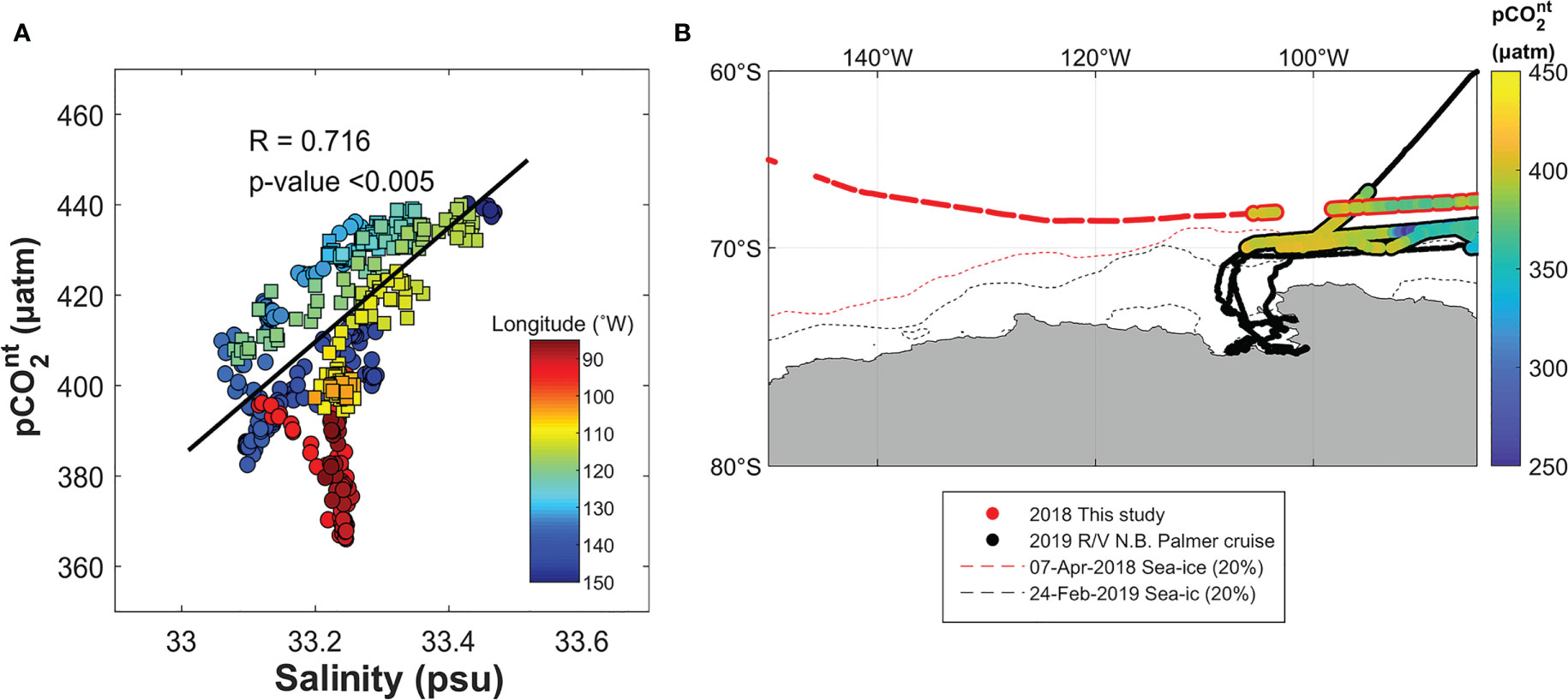
Figure 4 (A) Relationship between ${p\text{CO}}_2^{\text{nt}}$ and salinity in the ABS with longitude (colors). The ABS is divided into the marginal sea ice zone (i.e., from 100 to 130°W; squares) and an open area (circles). The regression line is determined using the results from 150 to 100°W. (B) Comparison between the distribution of non-thermal pCO₂ ( ${p\text{CO}}_2^{\text{nt}}$) obtained in this study (red solid line) and those reported in previous studies (black solid line) in the Amundsen-Bellingshausen Sea. The dashed lines in (B) indicate the sea ice edge determined in 2018 (red) and 2019 (black).

TABLE 4

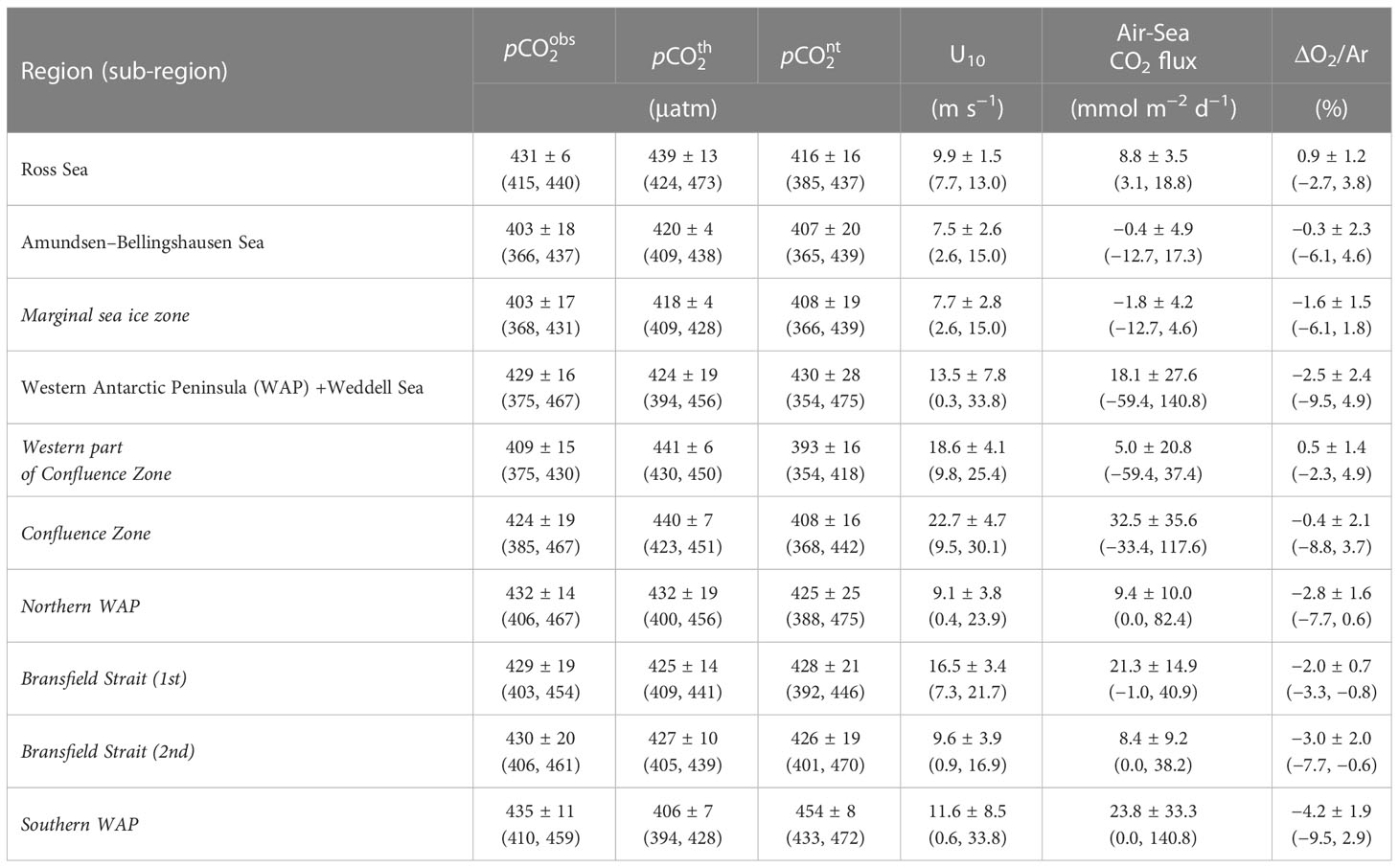
Table 4 Mean, standard deviation, ranges of underway pCO₂ (${p\text{CO}}_2^{\text{obs}}$), thermal pCO₂ (${p\text{CO}}_2^{\text{th}}$), non-thermal pCO₂ ( ${p\text{CO}}_2^{\text{nt}}$), wind speed at 10 m (U₁₀), air-sea CO₂ fluxes, and the difference in the gas ratios between oxygen and argon O₂/Ar values of the sample and air-saturated water (ΔO₂/Ar).

The air–sea CO₂ flux in the ABS ranged from −12.7 to 17.3 mmol m⁻² d⁻¹. Overall, the marginal sea ice zone of the ABS region acted as a weak CO₂ sink (−1.8 ± 4.2 mmol m⁻² d⁻¹) for atmospheric CO₂, whereas the open area served as a weak CO₂ source (0.9 ± 5.1 mmol m⁻² d⁻¹) during the study period (Figure 2E). According to previous studies, the air–sea CO₂ fluxes in the Amundsen Sea and Bellingshausen Sea range from −16 to 14 mmol m⁻² d⁻¹ (Tortell et al., 2012; Mu et al., 2014; Kim et al., 2018) and from −6.5 to 0 mmol m⁻² d⁻¹ (Álvarez et al., 2002; Ito et al., 2018), respectively, during summer. In particular, previous studies identified strong atmospheric CO₂ uptake in polynyas or areas with diatom blooms (Álvarez et al., 2002; Tortell et al., 2012). However, it is important to emphasize that in this study, significant CO₂ fluxes were observed due to high wind speeds, even when the pCO₂ difference between the atmosphere and ocean was small. (Figure 2E).

Western Antarctic Peninsular and Weddell sea sector

A large part of the WAP region belongs to the Bellingshausen Sea. However, in this study, we separated the WAP region from the rest of the Bellingshausen Sea to highlight the complex pCO₂ variations in the WAP/WS region. First, at the entrance (66°W–68°W in this study) of the WAP before arriving at the CZ zone, we found a sudden increase in the ΔO₂/Ar around the SB (Figure S3C). Thus, we expected that biological activities governed the pCO₂ variations in this region. Correlation analysis showed that ${p\text{CO}}_2^{\text{nt}}$was correlated with the SSS and ΔO₂/Ar in the south (66°W–68°W) and north (66°W–65.5°W) of the SB at the entrance of the WAP, respectively (Figure 5), similar to the results obtained from the NRS. The SSS–${p\text{CO}}_2^{\text{nt}}$relationship unlikely originated from the sea ice formation, because the entrance of the WAP was ice-free during the study period (Figure 1B). Shadwick et al. (2021) suggested that the MLD in the WAP gradually deepens from summer (~20 m in January) to winter (~100 m in November), and reported that the MLD is approximately 60 m in April (Panassa et al., 2018). Therefore, the high ${p\text{CO}}_2^{\text{nt}}$values in this region result from the intensification of the vertical mixing, which leads to the upwelling of CO₂-riched seawater from the subsurface layer.

FIGURE 5

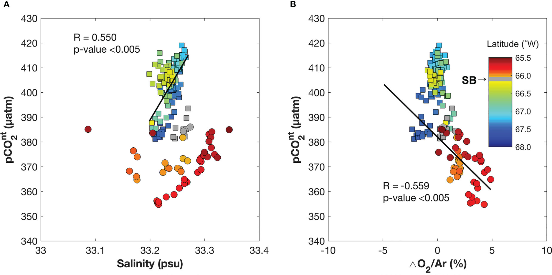
Figure 5 Relationship between non-thermal pCO₂ (${p\text{CO}}_2^{\text{nt}}$) and (A) salinity and (B) the difference in the gas ratios between oxygen and argon O₂/Ar values of the sample and air-saturated water (ΔO₂/Ar) in the western part of the Confluence Zone. This region is divided into northern (i.e.,<66.1°S) (squares) and southern (i.e., >66.1°S) parts (circles) based on the Southern Boundary (SB) of the Antarctic circumpolar current. The colors represent the latitude, and the gray color implies the latitude of the SB. The regression lines in (A, B) are determined based on the results obtained from the northern and southern parts, respectively.

In the CZ, various water masses originating from the Bellingshausen Sea, WS, and meteoric water are usually mixed (Meredith et al., 2013; Cook et al., 2016), resulting in the greatest variation in the SST and SSS compared to those in the other subregions. ${p\text{CO}}_2^{\text{nt}}$in this region was strongly inversely correlated with the ΔO₂/Ar (Figure 6). Despite overall heterotrophic condition (i.e., mean ΔO₂/Ar< 0), the CZ area showed the broadest variations (−8.8 to 3.7%) in ΔO₂/Ar, among the three subregions, indicating correlations between pCO₂ and the ΔO₂/Ar. The pCO₂ sensitivity to a given ΔO₂/Ar variation (i.e., a regression slope between ΔO₂/Ar and pCO₂) was similar in the CZ and NRS. Previous studies have demonstrated that the concentrations of dissolved organic carbon during summer range from 35 to 127 μmol kg^–1 in the Gerlache strait (between 64°S – 65°S and between 61°W – 64°W) (Doval et al., 2002; da Cunha et al., 2018) and from 44 to 64 μmol kg^–1 in the Bransfield Strait (Ruiz-Halpern et al., 2014). These values are relatively higher than or similar to those in the other regions; 38–56 μmol kg^–1 in the Ross Sea (Ogawa et al., 1999; Carlson et al., 2000; Bercovici et al., 2017) and approximately 44–63 μmol kg^–1 in the Amundsen Sea (Fang et al., 2020). The high accumulation of dissolved organic carbon suggests a potential for respiration-based CO₂ production in the CZ area.

FIGURE 6

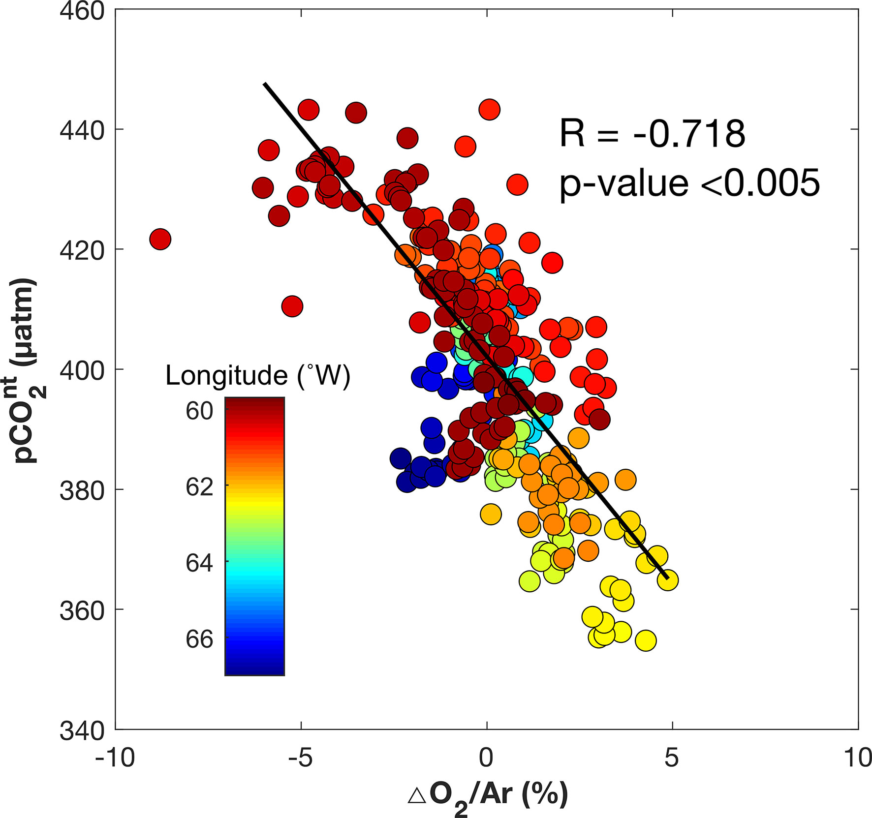
Figure 6 Relationship between non-thermal pCO₂ (${p\text{CO}}_2^{\text{nt}}$) and the difference in the gas ratios between oxygen and argon O₂/Ar values of the sample and air-saturated water (ΔO₂/Ar) in the Confluence Zone of the Western Antarctic peninsula with respect to the longitude (colors).

The transition between the N-WAP/WS and S-WAP/WS exhibited a sharp shift in pCO₂ (Figure 2C). ${p\text{CO}}_2^{\text{nt}}$(${p\text{CO}}_2^{\text{th}}$) in the N-WAP/WS was lower (higher) than that in the S-WAP/WS (mainly northwestern part of the Weddell Sea). The mean ${p\text{CO}}_2^{\text{obs}}$(${p\text{CO}}_2^{\text{nt}}$) values were 432 ± 14 (425 ± 25) and 435 ± 11 (454 ± 8) μatm in the N-WAP/WS and S-WAP/WS, respectively. In contrast, Ito et al. (2018) reported that pCO₂ in the N-WAP/WS (361 to 392 μatm) was higher than that in the Weddell Sea (343 to 376 μatm) during summer in 2008–2010. This inconsistency possibly results from the seasonal changes in the sea ice melting/formation and biological processes from summer to autumn. The chlorophyll-a concentration in the Weddell Sea was higher than that in the N-WAP/WS during the summers of 2008 and 2009 (Ito et al., 2018). However, from April 15 to April 30, the sea ice over most of the Weddell Sea increased by up to ~80% (Figure 1B). Consistently, the S-WAP/WS showed a slight SSS increase in April, relative to that observed in the study period of Ito et al. (2018). Combined with the reduced light availability, associated with the increased sea ice cover, brine rejection in the Weddell Sea during autumn likely caused the relatively high ${p\text{CO}}_2^{\text{obs}}$in the S-WAP/WS.

Two observations were conducted with a time interval of 14 days from the Trinity peninsula to the Maxwell Bay in the Bransfield Strait (Figures 1B, 7) to evaluate the mechanism underlying the effect of ice formation in the Weddell Sea on the pCO₂ variation in Bransfield Strait. Although the ocean current system in the Bransfield Strait is complex (Krechik et al., 2021), a relatively warm water mass that originates from the ACC and Bellingshausen Sea is generally introduced into the northern part of the Bransfield Strait. In contrast, relatively cold water from the Weddell Sea flows into the southern part of the Bransfield Strait. The north-to-south shift in ${p\text{CO}}_2^{\text{obs}}$and ${p\text{CO}}_2^{\text{nt}}$could be explained using the above-mentioned current system in the Bransfield Strait (Green shadings in Figure 2C). ${p\text{CO}}_2^{\text{nt}}$in the southern Bransfield Strait was lower than those in the northern Bransfield Strait during the first observation (BS1) (Figure 7A). However, during the second visit (BS2), ${p\text{CO}}_2^{\text{nt}}$was drastically elevated from< 400 μatm to >450 μatm, particularly in a part of the southern Bransfield Strait (near 63°S and 58°W) (Figure 7B). The SSS at 63°S and 58°W were 33.67 and 34.00 during the first and second observations, respectively. The SSS increase possibly originated from the corresponding increase in the SSS due to the enhanced sea ice concentration in the Weddell Sea. The values of ${p\text{CO}}_2^{\text{nt}}$in the northern boundary of the Bransfield Strait (i.e., close to the King George Island) during BS2 were higher than those found in the southern boundary of the Bransfield Strait, possibly due to the lower ΔO₂/Ar in the northern edge of the Bransfield Strait (Figure S3C). The mean ΔO₂/Ar in the northern (black box in Figure 7B) and southern (red box in Figure 7B) boundaries of the Bransfield Strait were –2.8 ± 1.6 and –4.2 ± 1.9%, respectively. The contribution of the water masses flowing from the ACC, Bellingshausen Sea, and Weddell Sea to the Bransfield Strait could be affected by the Southern Annual Mode (SAM). During the positive SAM period, contributions from the ACC and Bellingshausen Sea were more dominant, while the influence of the water masses from the Weddell Sea was dominant during the negative SAM period in the Bransfield strait (Vorrath et al., 2020). We speculate that the current from the Weddell Sea to the Bransfield strait increased in April 2018 because of the negative SAM index (–1.66) (Marshall, 2003).

FIGURE 7

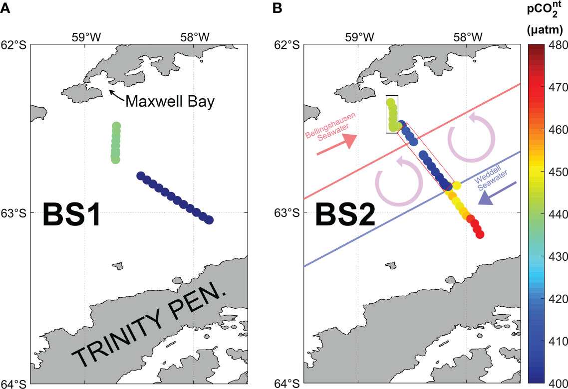
Figure 7 Comparison between the distribution of non-thermal pCO₂ (${p\text{CO}}_2^{\text{nt}}$): (A) first observation in the Bransfield Strait (BS1) and (B) second observation in the Bransfield Strait (BS2) in the Western Antarctic peninsula. The red and blue solid lines indicate the boundary of the Bellingshausen and Weddell seawaters, respectively. The boundaries are adapted from Sangrà et al. (2011). The red, blue, and purple arrows indicate the direction of the surface current.

Although the air–sea CO₂ flux in the WAP/WS considerably varied depending on the subregions, the WAP appeared to act as a CO₂ source (18.1 ± 27.6 mmol m⁻² d⁻¹) during this study (Table 4). The mean air–sea CO₂ flux was estimated to be 5.0 ± 20.8 mmol m⁻² d⁻¹ at the entrance of the WAP, 32.5 ± 35.6 mmol m⁻² d⁻¹ in the CZ, 9.4 ± 10.0 mmol m⁻² d⁻¹ in the N-WAP, and 23.8 ± 33.3 mmol m⁻² d⁻¹ in the S-WAP. In particular, the strong CO₂ emissions in the WAP/WS were caused by a high wind speed (13.5 ± 7.8 m s⁻¹). Álvarez et al. (2002) reported that a strong oceanic CO₂ uptake (−6.5 mmol m⁻² d⁻¹) occurred during summer due to the diatom bloom in the western WAP region (the northern part of CZ). A few researches also reported that the Bransfield Strait acted as an atmospheric CO₂ sink during spring and summer, with air–sea CO₂ fluxes ranging from −3.4 to 1.6 mmol m⁻² d⁻¹ (Ito et al., 2018; Caetano et al., 2020). Shadwick et al. (2021), who estimated the annual air–sea CO₂ flux using a mooring system suggested that the entrance of the WAP region acted as a CO₂ absorber in April, with an air–sea exchange of approximately −2 mmol m⁻² d⁻¹, which indicates potentially large temporal variations in this region.

Assessment of mechanisms for controlling pCO₂ in study regions

Our data indicate that non-thermal factors predominantly controlled pCO₂ in the Pacific sector of the Southern Ocean in April 2018, with the exception of the N-WAP/WS and S-WAP/WS (Figure 2). In the N-WAP/WS and S-WAP/WS, both thermal and non-thermal factors significantly influenced pCO₂. Williams et al. (2018) reported that biological processes primarily governed summer pCO₂ in the ASZ and SSIZ. Nevertheless, such predominant biology-driven control of pCO₂ was found in limited subregions, namely the southern SB of the NRS and the CZ of the WAP/WS regions. The SSS- ${p\text{CO}}_2^{\text{nt}}$correlation observed in the NRS, ABS, and entrance of WAP resulted from upwelling, sea ice formation, and enhanced vertical mixing in the NRS, ABS, and entrance of WAP, respectively. Our findings, distinct from those reported from summertime investigations, highlight the importance of cold-season observations. Our high-resolution data revealed a complex mechanism controlling pCO₂ in the Pacific sector of the Southern Ocean, suggesting that ship-based underway observations are essential for understanding the carbon cycle in the Antarctic waters.

Conclusions

Most observations of the ocean carbonate variables in the Southern Ocean have been conducted mainly during spring and summer because of improved accessibility. However, we conducted this study during a month in early autumn when field observations rarely cover most of the Pacific sector of the Southern Ocean, thus enhancing our understanding of the air–sea exchanges in the study area. Our data showed that physical processes (represented by salinity variation) and biological activities (explained by ΔO₂/Ar) are the dominant factors controlling ${p\text{CO}}_2^{\text{nt}}$in the western Antarctic Ocean. Previous studies have suggested that the Southern Ocean acts as a sink for atmospheric CO₂ from spring to early autumn (Álvarez et al., 2002; Ito et al., 2018; Caetano et al., 2020; Shadwick et al., 2021). However, we showed that this area acted as a source in April 2018, despite large spatial variations. This inconsistency indicates that further extensive research efforts are required in this study area.

Data availability statement

The datasets presented in this study can be found in online repositories. The names of the repository/repositories and accession number(s) can be found below: https://kpdc.kopri.re.kr/search/38a95561-58f4-4917-8583-a508310efd48 Korea polar data center (KPDC) KOPRI-KPDC-00002170.

Author contributions

AM analyzed the data and wrote the original draft. KP designed the study and contributed to field observations of pCO₂, and DH contributed to the ΔO₂/Ar measurements. JP and KK provided resources, JP and KP acted as project administrators. YK and JI helped with the pCO₂ data analysis. TK contributed in data analysis and manuscript writing. All authors contributed to the article and approved the submitted version.

Funding

This work was supported by the Carbon Cycle Change and Ecosystem Response under the Southern Ocean Warming (PE23110), Investigation of ice microstructure properties for developing low-temperature purification and environment/energy materials (PE23120), and Polar Academic Program (PE17900) funded by the Korea Polar Research Institute (KOPRI). Also, AM, YK, and TK acknowledges funding from the Mid-Career Researcher Program (2019R1A2C2089994) funded by the National Research Foundation of Korea.

Acknowledgments

The authors appreciate all the researchers and funding agencies. The authors would like to thank the IBRV ARAON captain and crew. This work was not possible without their valuable contribution to sample collection. The SOCCOM data were collected and made freely available by the Southern Ocean Carbon and Climate Observations and Modeling (SOCCOM) Project funded by the National Science Foundation, Division of Polar Programs (NSF PLR-1425989), supplemented by NOAA and NASA.

Conflict of interest

The authors declare that the research was conducted in the absence of any commercial or financial relationships that could be construed as a potential conflict of interest.

Publisher’s note

All claims expressed in this article are solely those of the authors and do not necessarily represent those of their affiliated organizations, or those of the publisher, the editors and the reviewers. Any product that may be evaluated in this article, or claim that may be made by its manufacturer, is not guaranteed or endorsed by the publisher.

Supplementary material

The Supplementary Material for this article can be found online at: https://www.frontiersin.org/articles/10.3389/fmars.2023.1192959/full#supplementary-material

References

Álvarez M., Rıíos A. F., Rosón G. (2002). Spatio-temporal variability of air–sea fluxes of carbon dioxide and oxygen in the bransfield and gerlache straits during austral summer 1995–96. Deep-Sea Res. II: Top. Stud. Oceanogr. 49, 643–662. doi: 10.1016/S0967-0645(01)00116-3

CrossRef Full Text | Google Scholar

Arrigo K. R., Lowry K. E., van Dijken G. L. (2012). Annual changes in sea ice and phytoplankton in polynyas of the amundsen Sea, Antarctica. Deep-Sea Res. II: Top. Stud. Oceanogr. 71-76, 5–15. doi: 10.1016/j.dsr2.2012.03.006

CrossRef Full Text | Google Scholar

Arrigo K. R., Van Dijken G. L. (2007). Interannual variation in air-sea CO₂ flux in the Ross Sea, Antarctica: a model analysis. J. Geophys. Res. Oceans 112, C3. doi: 10.1029/2006JC003492

CrossRef Full Text | Google Scholar

Arrigo K. R., van Dijken G. L., Bushinsky S. (2008). Primary production in the southern ocean 1997–2006. J. Geophys. Res. Oceans 113, C8. doi: 10.1029/2007jc004551

CrossRef Full Text | Google Scholar

Bates N. R., Hansell D. A., Carlson C. A., Gordon L. I. (1998). Distribution of CO₂ species, estimates of net community production, and air-sea CO2exchange in the Ross Sea polynya. J. Geophys. Res. Oceans 103:C2, 2883–2896. doi: 10.1029/97jc02473

CrossRef Full Text | Google Scholar

Bercovici S. K., Huber B. A., DeJong H. B., Dunbar R. B., Hansell D. A. (2017). Dissolved organic carbon in the Ross Sea: deep enrichment and export. Limnol. Oceanogr. 62, 2593–2603. doi: 10.1002/lno.10592

CrossRef Full Text | Google Scholar

Bushinsky S. M., Landschutzer P., Rodenbeck C., Gray A. R., Baker D., Mazloff M. R., et al. (2019). Reassessing southern ocean air-Sea CO₂ flux estimates with the addition of biogeochemical float observations. Global Biogeochem. Cycles 33, 1370–1388. doi: 10.1029/2019GB006176

PubMed Abstract | CrossRef Full Text | Google Scholar

Caetano L. S., Pollery R. C. G., Kerr R., Magrani F., Ayres Neto A., Vieira R., et al. (2020). High-resolution spatial distribution of pCO₂ in the coastal southern ocean in late spring. Antarct. Sci. 32, 476–485. doi: 10.1017/s0954102020000334

CrossRef Full Text | Google Scholar

Carlson C. A., Hansell D. A., Peltzer E. T., Smith W. O. Jr. (2000). Stocks and dynamics of dissolved and particulate organic matter in the southern Ross Sea, Antarctica. Deep-Sea Res. II: Top. Stud. Oceanogr. 47, 3201–3225. doi: 10.1016/S0967-0645(00)00065-5

CrossRef Full Text | Google Scholar

Carter B. R., Feely R. A., Williams N. L., Dickson A. G., Fong M. B., Takeshita Y. (2018). Updated methods for global locally interpolated estimation of alkalinity, pH, and nitrate. Liminol. Oceanogr.:Methods 16, 119–131. doi: 10.1002/lom3.10232

CrossRef Full Text | Google Scholar

Cook A. J., Holland P. R., Meredith M. P., Murray T., Luckman A., Vaughan D. G. (2016). Ocean forcing of glacier retreat in the western Antarctic peninsula. Science 353, 283–286. doi: 10.1126/science.aae0017

PubMed Abstract | CrossRef Full Text | Google Scholar

da Cunha L. C., Hamacher C., Farias C., d. O., Kerr R., Mendes C. R. B., et al. (2018). Contrasting end-summer distribution of organic carbon along the gerlache strait, northern Antarctic peninsula: bio-physical interactions. Deep-Sea Res. II: Top. Stud. Oceanogr. 149, 206–217. doi: 10.1016/j.dsr2.2018.03.003

CrossRef Full Text | Google Scholar

DeJong H. B., Dunbar R. B. (2017). Air-Sea CO₂ exchange in the Ross Sea, Antarctica. J. Geophys. Res. Oceans 122, 8167–8181. doi: 10.1002/2017jc012853

CrossRef Full Text | Google Scholar

DeJong H. B., Dunbar R. B., Koweek D. A., Mucciarone D. A., Bercovici S. K., Hansell D. A. (2017). Net community production and carbon export during the late summer in the Ross Sea, Antarctica. Global Biogeochem. Cycles 31, 473–491. doi: 10.1002/2016GB005417

CrossRef Full Text | Google Scholar

DeVries T. (2014). The oceanic anthropogenic CO₂ sink: storage, air-sea fluxes, and transports over the industrial era. Global Biogeochem. Cycles 28, 631–647. doi: 10.1002/2013gb004739

CrossRef Full Text | Google Scholar

Dickson A. G., Millero F. J. (1987). A comparison of the equilibrium constants for the dissociation of carbonic acid in seawater media. Deep-Sea Res. I: Oceanogr. Res. 34, 1733–1743. doi: 10.1016/0198-0149(87)90021-5

CrossRef Full Text | Google Scholar

Dlugokencky E. J., Mund J. W., Crotwell A. M., Crotwell M. J., Thoning K. W. (2021). Global Monitoring Laboratory repository. Data from: atmospheric carbon dioxide dry air mole fractions from the NOAA GML carbon cycle cooperative global air sampling network 1968-2020, version: 2021-07-30. doi: 10.15138/wkgj-f215

CrossRef Full Text | Google Scholar

Doval M. D., Álvarez-Salgado X. A., Castro C. G., Pérez F. F. (2002). Dissolved organic carbon distributions in the bransfield and gerlache straits, Antarctica. Deep-Sea Res. II: Top. Stud. Oceanogr. 49, 663–674. doi: 10.1016/S0967-0645(01)00117-5

CrossRef Full Text | Google Scholar

Eveleth R., Timmermans M. L., Cassar N. (2014). Physical and biological controls on oxygen saturation variability in the upper Arctic ocean. J. Geophys. Res. Oceans 119 (11), 7420–7432. doi: 10.1002/2014JC009816

CrossRef Full Text | Google Scholar

Fang L., Lee S., Lee S. A., Hahm D., Kim G., Druffel E. R., et al. (2020). Removal of refractory dissolved organic carbon in the amundsen Sea, Antarctica. Sci. Rep. 10, 1–8. doi: 10.1038/s41598-020-57870-6

PubMed Abstract | CrossRef Full Text | Google Scholar

Fay A. R., Lovenduski N. S., McKinley G. A., Munro D. R., Sweeney C., Gray A. R., et al. (2018). Utilizing the drake passage time-series to understand variability and change in subpolar southern ocean pCO₂. Biogeosciences 15, 3841–3855. doi: 10.5194/bg-15-3841-2018

CrossRef Full Text | Google Scholar

Fietzek P., Fiedler B., Steinhoff T., Körtzinger A. (2014). In situ quality assessment of a novel underwater pCO₂ sensor based on membrane equilibration and NDIR spectrometry. J. Atmos. Ocean. Technol. 31 (1), 181–196. doi: 10.1175/JTECH-D-13-00083.1

CrossRef Full Text | Google Scholar

Gregor L., Kok S., Monteiro P. (2017). Empirical methods for the estimation of southern ocean CO₂: support vector and random forest regression. Biogeosciences 14, 5551–5569. doi: 10.5194/bg-14-5551-2017

CrossRef Full Text | Google Scholar

Guéguen C., Tortell P. D. (2008). High-resolution measurement of southern ocean CO₂ and O₂/Ar by membrane inlet mass spectrometry. Mar. Chem. 108, 184–194. doi: 10.1016/j.marchem.2007.11.007

CrossRef Full Text | Google Scholar

Hill V. J., Light B., Steele M., Zimmerman R. C. (2018). Light availability and phytoplankton growth beneath Arctic sea ice: integrating observations and modeling. J. Geophys. Res. Oceans 123, 3651–3667. doi: 10.1029/2017JC013617

CrossRef Full Text | Google Scholar

Ito R. G., Tavano V. M., Mendes C. R. B., Garcia C. A. E. (2018). Sea-Air CO₂ fluxes and pCO₂ variability in the northern Antarctic peninsula during three summer periods, (2008–2010). Deep-Sea Res. II: Top. Stud. Oceanogr. 149, 84–98. doi: 10.1016/j.dsr2.2017.09.004

CrossRef Full Text | Google Scholar

Ito T., Woloszyn M., Mazloff M. (2010). Anthropogenic carbon dioxide transport in the southern ocean driven by ekman flow. Nature 463, 80–83. doi: 10.1038/nature08687

PubMed Abstract | CrossRef Full Text | Google Scholar

Johnson K. S., Jannasch H. W., Coletti L. J., Elrod V. A., Martz T. R., Takeshita Y., et al. (2016). Deep-Sea DuraFET: a pressure tolerant pH sensor designed for global sensor networks. Anal. Chem. 88, 3249–3256. doi: 10.1021/acs.analchem.5b04653

CrossRef Full Text | Google Scholar

Kim I., Hahm D., Park K., Lee Y., Choi J. O., Zhang M., et al. (2017). Characteristics of the horizontal and vertical distributions of dimethyl sulfide throughout the amundsen Sea polynya. Sci. Total. Environ. 584, 154–163. doi: 10.1016/j.scitotenv.2017.01.165

PubMed Abstract | CrossRef Full Text | Google Scholar

Kim B., Lee S., Kim M., Hahm D., Rhee T. S., Hwang J. (2018). An investigation of gas exchange and water circulation in the amundsen Sea based on dissolved inorganic radiocarbon. Geophys. Res. Lett. 45, 12,368–312,375. doi: 10.1029/2018gl079464

CrossRef Full Text | Google Scholar

Ko Y. H., Seok M. W., Jeong J. Y., Noh J. H., Jeong J., Mo A., et al. (2022). Monthly and seasonal variations in the surface carbonate system and air–sea CO₂ flux of the yellow Sea. Mar. pollut. Bull. 181, 113822. doi: 10.1016/j.marpolbul.2022.113822

PubMed Abstract | CrossRef Full Text | Google Scholar

Krechik V. A., Frey D. I., Morozov E. G. (2021). Peculiarities of water circulation in the central part of the bransfield strait in January 2020. Dokl. Earth Sci. 496, 92–95. doi: 10.1134/S1028334X21010116

CrossRef Full Text | Google Scholar

Lannuzel D., Tedesco L., Van Leeuwe M., Campbell K., Flores H., Delille B., et al. (2020). The future of Arctic sea-ice biogeochemistry and ice-associated ecosystems. Nat. Clim. Change 10, 983–992. doi: 10.1038/s41558-020-00940-4

CrossRef Full Text | Google Scholar

Lewis E. R., Wallace D. W. R. (1998). “Data from: program developed for CO2 system calculations (No. cdiac: CDIAC-105),” in Environmental system science data infrastructure for a virtual ecosystem. (ESS-DIVE repository). doi: 10.15485/1464255

CrossRef Full Text | Google Scholar

Lovenduski N. S., Fay A. R., McKinley G. A. (2015). Observing multidecadal trends in southern ocean CO₂ uptake: what can we learn from an ocean model? Global Biogeochem. Cycles 29, 416–426. doi: 10.1002/2014gb004933

CrossRef Full Text | Google Scholar

Macdonald A. M., Wanninkhof R., Dickson A. G., Swift J. H., Carlson C. A., Key R. M., et al. (2021). National Centers for Environmental Information repository. Data from: discrete profile measurements of dissolved inorganic carbon, total alkalinity, pH on total scale and other hydrographic and chemical parameters obtained during the R/V Nathaniel b. palmer repeat hydrography and SOCCOM cruise NBP18_02 in the pacific sector of southern ocean: GO-SHIP section S04P (EXPOCODE 320620180309), from 2018-03-09 - 2018-05-14 (NCEI accession 0225497). (National Centers for Environmental Information repository). doi: 10.25921/8arx-2058

CrossRef Full Text | Google Scholar

Macovei V. A., Voynova Y. G., Becker M., Triest J., Petersen W. (2021). Long-term intercomparison of two pCO₂ instruments based on ship-of-opportunity measurements in a dynamic shelf sea environment. Limnol. Oceanogr. Methods 19, 37–50. doi: 10.1002/lom3.10403

CrossRef Full Text | Google Scholar

Marrec P., Cariou T., Latimier M., Macé E., Morin P., Vernet M., et al. (2014). Spatio-temporal dynamics of biogeochemical processes and air–sea CO₂ fluxes in the Western English channel based on two years of FerryBox deployment. J. Mar. Syst. 140, 26–38. doi: 10.1016/j.jmarsys.2014.05.010

CrossRef Full Text | Google Scholar

Marshall G. J. (2003). Trends in the southern annular mode from observations and reanalyses. J. Clim. 16, 4134–4143. doi: 10.1175/1520-0442(2003)016<4134:TITSAM>2.0.CO;2

CrossRef Full Text | Google Scholar

Maslanik J., Stroeve J. (1999). National Snow and Ice Data Center repository. Data from: near-real-time DMSP SSM/I-SSMIS daily polar gridded sea ice concentrations. (National Snow and Ice Data Center repository). doi: 10.5067/U8C09DWVX9LM

CrossRef Full Text | Google Scholar

McNeil B. I., Metzl N., Key R. M., Matear R. J., Corbiere A. (2007). An empirical estimate of the southern ocean air-sea CO₂ flux. Global Biogeochem. Cycles 21, GB3011. doi: 10.1029/2007gb002991

CrossRef Full Text | Google Scholar

Mehrbach C., Culberson C. H., Hawley J. E., Pytkowicx R. M. (1973). Measurement of the apparent dissociation constants of carbonic acid in seawater at atmospheric pressure 1. Limnol. Oceanogr. 18, 897–907. doi: 10.4319/lo.1973.18.6.0897

CrossRef Full Text | Google Scholar

Meredith M. P., Venables H. J., Clarke A., Ducklow H. W., Erickson M., Leng M. J., et al. (2013). The freshwater system west of the Antarctic peninsula: spatial and temporal changes. J. Clim. 26, 1669–1684. doi: 10.1175/JCLI-D-12-00246.1

CrossRef Full Text | Google Scholar

Mikaloff Fletcher S. E., Gruber N., Jacobson A. R., Doney S. C., Dutkiewicz S., Gerber M., et al. (2006). Inverse estimates of anthropogenic CO₂ uptake, transport, and storage by the ocean. Global Biogeochem. Cycles 20, GB2002. doi: 10.1029/2005gb002530

CrossRef Full Text | Google Scholar

Millero F. J. (1995). Thermodynamics of the carbon dioxide system in the oceans. Geochim. Cosmochim. Acta 59, 661–677. doi: 10.1016/0016-7037(94)00354-O

CrossRef Full Text | Google Scholar

Mo A., Yang E. J., Kang S. H., Kim D., Lee K., Ko Y. H., et al. (2022). Impact of sea ice melting on summer air-sea CO₂ exchange in the East Siberian Sea. Front. Mar. Sci. 9. doi: 10.3389/fmars.2022.766810

PubMed Abstract | CrossRef Full Text | Google Scholar

Monteiro T., Kerr R., Machado E. D. C. (2020). Seasonal variability of net sea-air CO₂ fluxes in a coastal region of the northern Antarctic peninsula. Sci. Rep. 10, 14875. doi: 10.1038/s41598-020-71814-0

PubMed Abstract | CrossRef Full Text | Google Scholar

Moreau S., Vancoppenolle M., Bopp L., Aumont O., Madec G., Delille B., et al. (2016). Assessment of the sea-ice carbon pump: insights from a three-dimensional ocean-sea-ice biogeochemical model (NEMO-LIM-PISCES) assessment of the sea-ice carbon pump. Elem. Sci. Anth. 4, 000122. doi: 10.12952/journal.elementa.000122

CrossRef Full Text | Google Scholar

Mu L., Stammerjohn S. E., Lowry K. E., Yager P. L., Deming J. W., Miller L. A. (2014). Spatial variability of surface pCO2 and air-sea CO₂ flux in the amundsen Sea polynya, Antarctica. Elem. Sci. Anth 3, 000036. doi: 10.12952/journal.elementa.000036

CrossRef Full Text | Google Scholar

Nevison C. D., Manizza M., Keeling R. F., Stephens B. B., Bent J. D., Dunne J., et al. (2016). Evaluating CMIP5 ocean biogeochemistry and southern ocean carbon uptake using atmospheric potential oxygen: present-day performance and future projection. Geophys. Res. Lett. 43, 2077–2085. doi: 10.1002/2015GL067584

CrossRef Full Text | Google Scholar

Ogawa H., Fukuda R., Koike I. (1999). Vertical distributions of dissolved organic carbon and nitrogen in the southern ocean. Deep-Sea Res. I: Oceanogr. Res. 46, 1809–1826. doi: 10.1016/S0967-0637(99)00027-8

CrossRef Full Text | Google Scholar

Orr J. C., Maier-Reimer E., Mikolajewicz U., Monfray P., Sarmiento J. L., Toggweiler J. R., et al. (2001). Estimates of anthropogenic carbon uptake from four three-dimensional global ocean models. Global Biogeochem. Cycles 15, 43–60. doi: 10.1029/2000gb001273

CrossRef Full Text | Google Scholar

Panassa E., Völker C., Wolf-Gladrow D., Hauck J. (2018). Drivers of interannual variability of summer mixed layer depth in the southern ocean between 2002 and 2011. J. Geophys. Res. Oceans 123, 5077–5090. doi: 10.1029/2018JC013901

CrossRef Full Text | Google Scholar

Park Y. H., Durand I. (2019). “Data from: altimetry-drived Antarctic circumpolar current fronts,” in SEANOE repository. Available at: https://www.seanoe.org/data/00486/59800/.

Google Scholar

Rigual-Hernández A. S., Trull T. W., Bray S. G., Cortina A., Armand L. K. (2015). Latitudinal and temporal distributions of diatom populations in the pelagic waters of the subantarctic and polar frontal zones of the southern ocean and their role in the biological pump. Biogeosciences 12, 5309–5337. doi: 10.5194/bg-12-5309-2015

CrossRef Full Text | Google Scholar

Rivaro P., Ianni C., Langone L., Ori C., Aulicino G., Cotroneo Y., et al. (2017). Physical and biological forcing of mesoscale variability in the carbonate system of the Ross Sea (Antarctica) during summer 2014. J. Mar. Syst. 166, 144–158. doi: 10.1016/j.jmarsys.2015.11.002

CrossRef Full Text | Google Scholar

Robertson J. E., Watson A. J. (1995). A summer-time sink for atmospheric carbon dioxide in the southern ocean between 88 W and 80 e. Deep-Sea Res. II: Top. Stud. Oceanogr. 42, 1081–1091. doi: 10.1016/0967-0645(95)00067-Z

CrossRef Full Text | Google Scholar

Ruiz-Halpern S., Calleja M. L., Dachs J., Del Vento S., Pastor M., Palmer M., et al. (2014). Ocean–atmosphere exchange of organic carbon and CO₂ surrounding the Antarctic peninsula. Biogeosciences 11, 2755–2770. doi: 10.5194/bg-11-2755-2014

CrossRef Full Text | Google Scholar

Sangrà P., Gordo C., Hernandez-Arencibia M., Marrero-Díaz A., Rodríguez-Santana A., Stegner A., et al. (2011). The bransfield current system. Deep-Sea Res. I: Oceanogr. Res. Pap. 58, 390–402. doi: 10.1016/j.dsr.2011.01.011

CrossRef Full Text | Google Scholar

Schulze Chretien L. M., Thompson A. F., Flexas M. M., Speer K., Swaim N., Oelerich R., et al. (2021). The shelf circulation of the bellingshausen Sea. J. Geophys. Res. Oceans 126, e2020JC016871. doi: 10.1029/2020jc016871

CrossRef Full Text | Google Scholar

Shadwick E. H., De Meo O. A., Schroeter S., Arroyo M. C., Martinson D. G., Ducklow H. (2021). Sea Ice suppression of CO₂ outgassing in the West Antarctic peninsula: implications for the evolving southern ocean carbon sink. Geophys. Res. Lett. 48, e2020GL091835. doi: 10.1029/2020gl091835

CrossRef Full Text | Google Scholar

Sokolov S., Rintoul S. R. (2007). On the relationship between fronts of the Antarctic circumpolar current and surface chlorophyll concentrations in the southern ocean. J. Geophys. Res. 112, C7. doi: 10.1029/2006jc004072

CrossRef Full Text | Google Scholar

Speer K., Rintoul S. R., Sloyan B. (2000). The diabatic deacon cell. J. Phys. Oceanogr. 30, 3212–3222. doi: 10.1175/1520-0485(2000)030<3212:TDDC>2.0.CO;2

CrossRef Full Text | Google Scholar

Sutherland S. C., Newberger T., Takahashi T., Sweeney C. (2019) Data from: report of underway pCO2 measurements in surface waters and the atmosphere during feburary-march 2019, R/V Nathaniel B.Palmer cruise 19/2. Available at: https://www.ldeo.columbia.edu/res/pi/CO2/carbondioxide/pages/2019palmer.html.

Google Scholar

Sutton A. J., Williams N. L., Tilbrook B. (2021). Constraining southern ocean CO₂ flux uncertainty using uncrewed surface vehicle observations. Geophys. Res. Lett. 48, e2020GL091748. doi: 10.1029/2020gl091748

CrossRef Full Text | Google Scholar

Takahashi T., Olafsson J., Goddard J. G., Chipman D. W., Sutherland S. C. (1993). Seasonal variation of CO₂ and nutrients in the high-latitude surface oceans: a comparative study. Glob. Biogeochem. Cycles. 7, 843–878. doi: 10.1029/93GB02263

CrossRef Full Text | Google Scholar

Takahashi T., Sutherland S. C., Sweeney C., Poisson A., Metzl N., Tilbrook B., et al. (2002). Global sea–air CO₂ flux based on climatological surface ocean pCO₂, and seasonal biological and temperature effects. Deep-Sea Res. II: Top. Stud. Oceanogr. 49, 1601–1622. doi: 10.1016/S0967-0645(02)00003-6

CrossRef Full Text | Google Scholar

Takahashi T., Sutherland S. C., Wanninkhof R., Sweeney C., Feely R. A., Chipman D. W., et al. (2009). Climatological mean and decadal change in surface ocean pCO₂, and net sea–air CO₂ flux over the global oceans. Deep-Sea Res. II: Top. Stud. Oceanogr. 56, 554–577. doi: 10.1016/j.dsr2.2008.12.009

CrossRef Full Text | Google Scholar

Thomas B. R., Kent E. C., Swail V. R. (2005). Methods to homogenize wind speeds from ships and buoys. Int. J. Climatol. 25, 979–995. doi: 10.1002/joc.1176

CrossRef Full Text | Google Scholar

Tortell P. D., Guéguen C., Long M. C., Payne C. D., Lee P., DiTullio G. R. (2011). Spatial variability and temporal dynamics of surface water pCO₂, ΔO₂/Ar and dimethylsulfide in the Ross Sea, Antarctica. Deep-Sea Res. I: Oceanogr. Res. 58, 241–259. doi: 10.1016/j.dsr.2010.12.006

CrossRef Full Text | Google Scholar

Tortell P. D., Long M. C., Payne C. D., Alderkamp A.-C., Dutrieux P., Arrigo K. R. (2012). Spatial distribution of pCO₂, ΔO₂/Ar and dimethylsulfide (DMS) in polynya waters and the sea ice zone of the amundsen Sea, Antarctica. Deep-Sea Res. II: Top. Stud. Oceanogr. 71, 77–93. doi: 10.1016/j.dsr2.2012.03.010

CrossRef Full Text | Google Scholar

Totland C., Eek E., Blomberg A. E., Waarum I. K., Fietzek P., Walta A. (2020). The correlation between pO2 and pCO₂ as a chemical marker for detection of offshore CO₂ leakage. Int. J. Greenh. Gas Control 99, 103085. doi: 10.1016/j.ijggc.2020.103085

CrossRef Full Text | Google Scholar

Vorrath M.-E., Müller J., Rebolledo L., Cárdenas P., Shi X., Esper O., et al. (2020). Sea Ice dynamics in the bransfield strait, Antarctic peninsula, during the past 240 years: a multi-proxy intercomparison study. Clim. Past 16, 2459–2483. doi: 10.5194/cp-16-2459-2020

CrossRef Full Text | Google Scholar

Wadhams P. (1986). “The seasonal ice zone,” in The geophysics of Sea ice. Ed. Untersteiner N. (Boston, MA: Springer). doi: 10.1007/978-1-4899-5352-0_15

CrossRef Full Text | Google Scholar

Wanninkhof R. (2014). Relationship between wind speed and gas exchange over the ocean revisited. Limnol. Oceanogr. Methods 12, 351–362. doi: 10.4319/lom.2014.12.351

CrossRef Full Text | Google Scholar

Weiss R. (1974). Carbon dioxide in water and seawater: the solubility of a non-ideal gas. Mar. Chem. 2, 203–215. doi: 10.1016/0304-4203(74)90015-2

CrossRef Full Text | Google Scholar

Williams N. L., Juranek L. W., Feely R. A., Johnson K. S., Sarmiento J. L., Talley L. D., et al. (2017). Calculating surface ocean pCO₂ from biogeochemical argo floats equipped with pH: an uncertainty analysis. Global Biogeochem. Cycles 31, 591–604. doi: 10.1002/2016gb005541

CrossRef Full Text | Google Scholar

Williams N. L., Juranek L. W., Feely R. A., Russell J. L., Johnson K. S., Hales B. (2018). Assessment of the carbonate chemistry seasonal cycles in the southern ocean from persistent observational platforms. J. Geophys. Res. Oceans 123, 4833–4852. doi: 10.1029/2017jc012917

CrossRef Full Text | Google Scholar

Zhang J., Spitz Y. H., Steele M., Ashjian C., Campbell R., Berline L., et al. (2010). Modeling the impact of declining sea ice on the Arctic marine planktonic ecosystem. J. Geophys. Res. Oceans 115, C10. doi: 10.1029/2009JC005387

CrossRef Full Text | Google Scholar