Uncertainties in wave-driven longshore sediment transport projections presented by a dynamic CMIP6-based ensemble

In this study four experiments were conducted to investigate uncertainty in future longshore sediment transport (LST) projections due to: working with continuous time series of CSIRO CMIP6-driven waves (experiment #1) or sliced time series of waves from CSIRO-CMIP6-Ws and CSIRO-CMIP5-Ws (experiment #2); different wave-model-parametrization pairs to generate wave projections (experiment #3); and the inclusion/exclusion of sea level rise (SLR) for wave transformation (experiment #4). For each experiment, a weighted ensemble consisting of offshore wave forcing conditions, a surrogate model for nearshore wave transformation and eight LST models was used. The results of experiment # 1 indicated that the annual LST rates obtained from a continuous time series of waves were influenced by climate variability acting on timescales of 20-30 years. Uncertainty decomposition clearly reveals that for near-future coastal planning, a large part of the uncertainty arises from model selection and natural variability of the system (e.g., on average, 4% scenario, 57% model, and 39% internal variability). For the far future, the total uncertainty consists of 25% scenario, 54% model and 21% internal variability. Experiment #2 indicates that CMIP6 driven wave climatology yield similar outcomes to CMIP5 driven wave climatology in that LST rates decrease along the study area’s coast by less than 10%. The results of experiment #3 indicate that intra- and inter-annual variability of LST rates are influenced by the parameterization schemes of the wave simulations. This can increase the range of uncertainty in the LST projections and at the same time can limit the robustness of the projections. The inclusion of SLR (experiment #4) in wave transformation, under SSP1-2.6 and SSP5-8.5 scenarios, yields only meagre changes in the LST projections, compared to the case no SLR. However, it is noted that future research on SLR influence should include potential changes in nearshore profile shapes.

1 Introduction

Along open sandy coasts, breaking waves and the resulting alongshore currents drive longshore sediment transport (LST). LST processes play a significant role on long-term (e.g., interannual to decadal) coastal evolution of sandy coasts (Anderson et al., 2018; Antolínez et al., 2018). The success of coastal engineering and management projects, such as beach nourishment (e.g., Stronkhorst et al., 2018), port layout (OCDI, 2009), sand by-passing/back-passing systems (e.g., Vieira da Silva et al., 2021), and integrated shoreline management planning (Mangor et al., 2017), relies on the accurate measurement and prediction of LST rates, longshore gradients and cross-shore distribution. Generally, providing reliable estimates of the sediment transport patterns is still a challenge, as forcing conditions and sediment transport processes through modelling frameworks are prone to intra and inter-model uncertainties (i.e., arising from different models and/or different settings) (D’Anna et al., 2020; Kroon et al., 2020; Chataigner et al., 2022; Zarifsanayei et al., 2022a). Additionally, providing reliable measurements of LST patterns for model calibration is quite challenging (Cooper and Pilkey, 2007). It is important to note that uncertainty growth in the hindcast of LST patterns is relatively manageable through development of state-of-the-art strategies (e.g., better understanding of coastal processes, employing new generation models, using extensive benchmark data, calibration, etc.). However, narrowing uncertainty in the projection of LST patterns (i.e., future patterns of LST) is more challenging (Vitousek et al., 2021; Zarifsanayei et al., 2022b).

Long-term coastal management planning requires quantitative and qualitative estimates of climate change impacts on sediment transport and coastal evolution patterns (Ranasinghe, 2016; Toimil et al., 2020; Toimil et al., 2021). In response to global warming, future wind-wave forcing conditions can change, yielding significant variations in the patterns of sediment transport (Ruggiero et al., 2010; Sierra and Casas-Prat, 2014; Zarifsanayei et al., 2020). The effect of global warming on the wind-wave climate by the end of 21^st century has been widely studied (e.g., Semedo et al., 2012; Hemer et al., 2013; Hemer and Trenham, 2016; Camus et al., 2017; Morim et al., 2019; Lemos et al., 2020a, Lemos et al., 2020b; Lemos et al., 2021). However, the uncertainty ranges of the projected wave climate patterns, presented by different global wave modelling efforts (i.e., CMIP3-, CMIP5-, and CMIP6-forced wave simulations) varies due to differences in assumed emission scenario pathways [e.g., Assessment Reports (AR) 3, 5, and 6 from the Intergovernmental Panel on Climate Change (IPCC), along with the Special Report on Emissions Scenarios (SRES), Representative Concentration Pathways (RCPs), and Shared Socio-economic Pathways (SSPs)]. Uncertainty also arises due to the implementation of different model combinations as models evolve (i.e., Global Circulation Models (GCMs) and wave models) under different physics/settings/resolutions. The release of new, CMIP6-driven wave climate datasets allows for the investigation of the SSPs emission scenarios, the role of spatio-temporal resolutions of forcing conditions, as well as the impacts of different wind-wave parametrizations within the wave models on wave climate projections outputs (Kumar et al., 2022).

Recently, the potential impact of climate change on wave-driven LST patterns has been studied in different regions (e.g., central coast of England, Zacharioudaki and Reeve, 2011; a stretch of coast in Italy, Bonaldo et al., 2015; West Africa coastline, Almar et al., 2015; Spanish coasts, Casas-Prat et al., 2016; Vietnam Coasts, Dastgheib et al., 2016; a short stretch of coast in southern Australia, O’Grady et al., 2019; Northwest of Portugal, Fernández-Fernández et al., 2020; Indian Coast, Chowdhury et al., 2020). A few studies (e.g., Zacharioudaki and Reeve, 2011) tried to manipulate the historical wave patterns to mimic climate change impacts on future wave and sediment transport patterns. For example, changes in mean wave direction, and patterns of storms were defined from the historical record and then the historical wave forcings were modified and used to force a sediment transport model to project changes in sediment transport patterns into the future (e.g., Ruggiero et al., 2010). Although such an approach can show the sensitivity of sediment transport and coastal evolution to potential changes in wave climate, relying only on this method for coastal planning is limited because it relies on historical trends in wave climate. Hence, an approach using GCM-forced wave simulations (GCM-Ws) under greenhouse gas emission scenarios, has been increasingly adopted in literature to project future patterns of wave climate (e.g., Morim et al., 2019; Meucci et al., 2020). However, due to large computational costs of wave simulations, only a limited number of datasets were used in the literature. Similarly, for the projection of LST patterns, due to computational limitations, the use of process-based sediment transport models has been less frequent (e.g., Bonaldo et al., 2015; O’Grady et al., 2019), and the use of simplified models (bulk formulas) has been generally preferred. The aforementioned efforts could only partly address the uncertainty in the LST projections due to limited sampling and quantification of the uncertainty space.

More recently, Zarifsanayei et al. (2022b) quantified uncertainty in LST projections for a non-straight coastline (Gold Coast, Australia) using a more comprehensive sample of the uncertainty space. They developed two ensembles, formed by original and bias-corrected wave datasets of CSIRO CMIP5 (eight sets of GCM-Ws) projected under two emission scenarios, a hybrid wave-transformation method, and eight sediment transport models (including both bulk formula and process-based models). Additionally, they employed a novel scheme for weighting the ensemble members and explored the robustness of the LST projections. They acknowledged the need to use ensembles using a variety of GCM-W datasets projected under different emission scenarios (at least one optimistic and one pessimistic scenario). They have shown that a large portion of total uncertainty in the LST projections (over 80%) was controlled by the selection of emission scenarios and GCM-Ws, and their nonlinear interactions. This finding leads us to question the reliability of any sediment transport projections in which only a few GCM-Ws under one emission scenario arbitrarily were chosen. Moreover, their results implied that although applying bias correction techniques to wave forcings and weighting the ensembles’ members together could relatively reduce the range of uncertainty in LST projections, still no robust projected changes in the LST patterns on annual and seasonal scales were obtained.

Addressing the uncertainty in LST projections is a vital step toward the development of more reliable frameworks for projecting future coastal erosion and accretion patterns. Despite previous efforts, there are some uncertainty sources in LST projections that are yet to be considered. For instance, differences between CMIP5 and CMIP6 experiments, long-term (>100yr) continuous projections versus block time slice projections, spatio-temporal resolution and emission scenario definitions may have a significant influence on the projection of wave-driven LST patterns. The use of different parameterization schemes for wind-wave processes within the wave models (or even different wave models), has shown to be a source of uncertainty in projecting offshore waves (Kumar et al., 2022). The impact of this issue on LST patterns is also yet unknown. Moreover, the inclusion of the influence of Sea Level Rise (SLR) on wave transformation, where nearshore bathymetry is relatively complex, might change the wave dissipation patterns and the resulting LST patterns. This study aims to address these knowledge gaps using experiments developed using newly available CMIP6-driven wave simulations with the Gold Coast, Australia selected as the study site (Zarifsanayei et al., 2022a; 2022b). In particular, the experiments were designed to investigate the following aspects of uncertainty:

1. The trend of LST patterns presented by continuous time series of waves projected under two SSPs and decomposition of total uncertainty of LST projections into internal variability, emission scenario and model uncertainties;

2. Using block time slices waves to compare uncertainty within CSIRO-CMIP6-Ws driven LST rates, with that of CSIRO-CMIP5-Ws driven LST rates;

3. Uncertainty in the LST projections due to employing an ensemble of offshore waves driven by a single GCM under a single SSP but obtained from different schemes of wind-wave parametrizations (i.e., presented by different spectral wave models/parametrizations); and

4. Wave transformation uncertainty arising from inclusion or exclusion of SLR and its implications for the projection of wave-driven sediment transport under SSP1-2.6 and SSP5-8.5.

2 Methodology

The basis of each of the four experiments is to form an ensemble of forcing conditions (GCM-Ws under one or two SSPs), a surrogate wave model for nearshore wave transformation and eight sediment transport models to capture the range of uncertainty. The methodology of each experiment is illustrated in Figures 1, 2.

FIGURE 1

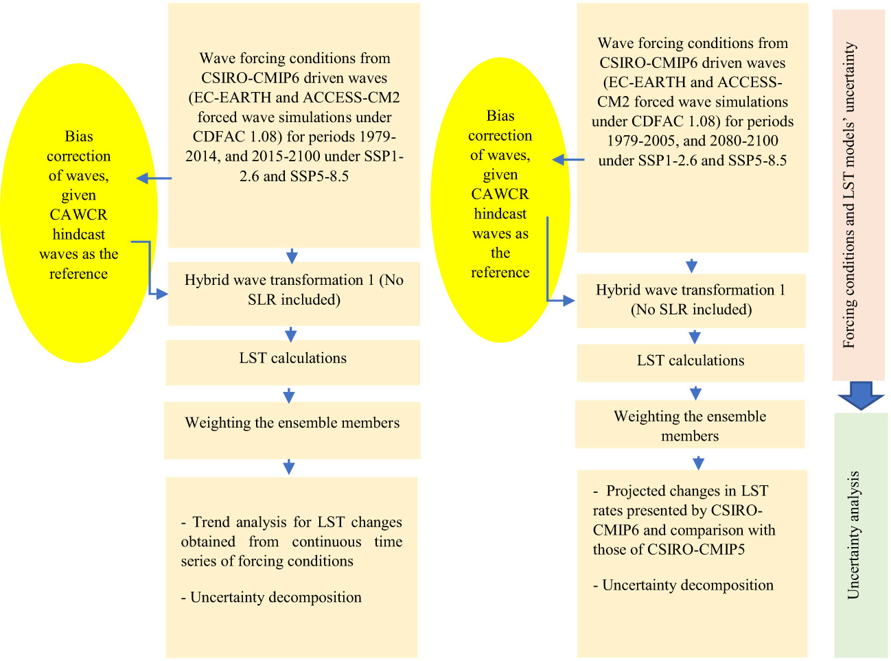
Figure 1 Methodology adopted for experiment # 1 (left panel) and experiment # 2 (right panel).

FIGURE 2

Figure 2 Methodology adopted for experiment #3 (left panel) and experiment # 4 (right panel).

2.1 Study site

The coastal city of the Gold Coast (GC) is located in southeast Queensland, Australia and has a 35-km sandy shoreline covering a range of coastline types including sheltered, semi-sheltered, and open coasts (see Figure 3). For decades, coastal erosion and sediment deficit have been the main challenges for coastal management in this region and consequently the GC shoreline is one of the most highly engineered sites around the world. The coastal erosion problem is mitigated by periodic beach nourishment, permanent sand by-passing systems operating at the north and south of Gold Coast, and a back-passing system to better manage the northern Gold Coast beaches (DHL, 1992; Vieira da Silva et al., 2021). Moreover, to protect the city from storm surges and wave action, the coastline is backed by a sea wall buried under a primary man-made dune system. The whole coastline is made of medium to fine, well sorted and uniformly distributed sand. Offshore waves are predominantly from the south to south-easterly directions which results in a significant northwards LST with the annual average net northward LST rate of 635,000 m³ at the northern end of the coast (GCCM, 2017).

FIGURE 3

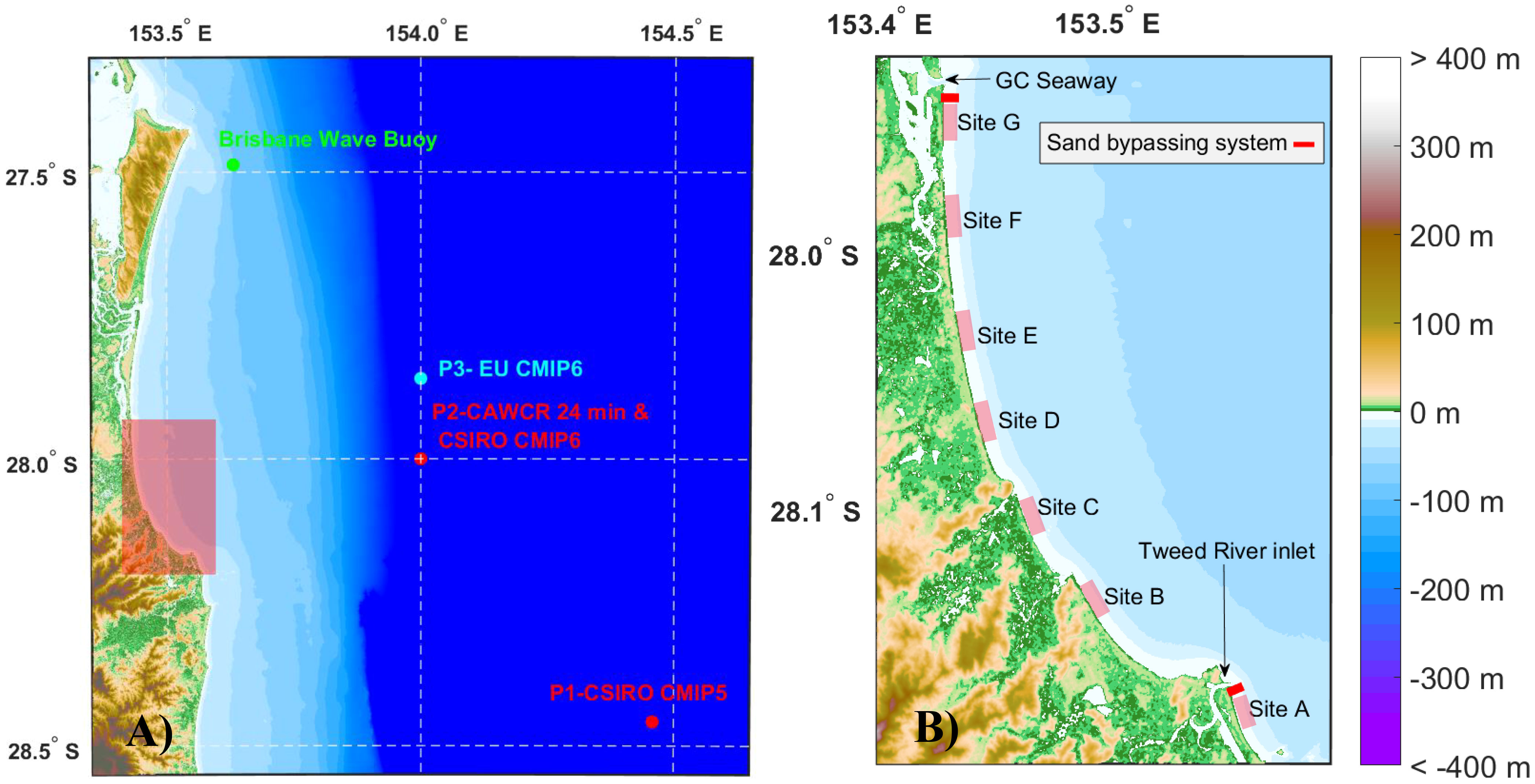
Figure 3 (A) Study area (Gold Coast region; highlighted) and locations of wave data; (B) Location of sites selected for LST projections (adopted from Zarifsanayei et al., 2022b).

Three distinct seasons can be defined for the offshore wave climate system of this region (City of Gold Coast, 2015; Zarifsanayei et al., 2022a). During summer (December-May), wave energy is from the east to south-easterly directions. During winter (June-August), offshore waves are more from the south to south-easterly directions in response to the intensification of Southern Ocean weather patterns. Spring (September-November) is normally characterised by calmer conditions. In most seasons, extreme storms can be generated in the Tasman Sea or Coral Sea and cause severe erosion. Local wind forcing such as sea breezes exist, however due to limited information and data its influence on local wave transformation is unknown.

Along the GC, nearshore wave climate patterns vary due to changes in coastline orientation and refraction patterns. The southern beaches are mainly semi-sheltered or sheltered, facing north and thus less exposed to the predominant swells coming from the south and southeast. However, the northern beaches (with east-facing coasts) are more exposed to offshore swell wave energy approaching the coast from all directions (Vieira Da Silva et al., 2018). The present study utilises the same modelling framework of (Zarifsanayei et al., 2022a, Zarifsanayei et al., 2022b), where seven sites along the GC shoreline were selected for investigation of uncertainty in the LST projections at sheltered (site B), semi-sheltered (sites A and C) and open coast locations (sites D to G; see Figure 3, which also shows the locations of offshore wave data buoys).

2.2 Projected offshore wave datasets

Two datasets of projected offshore waves (GCM-Ws) were used in this study namely, the CSIRO- CMIP6 wave data (CSIRO-CMIP6-Ws; Meucci et al., 2022) and EU wave data (EU-Ws; Lemos et al., 2023). Integrated parameter data from the nearest grid point to the Gold Coast (see Figure 3A) was extracted from each dataset and used as the offshore boundary condition of the local wave transformation model (cf. section 2.3).

The CSIRO-CMIP6-Ws datasets consist of archived 3-hourly outputs from a WaveWatchIII (WW3) model run on a 0.5 deg global grid. WW3 was run with the latest observation-based source term parametrization ST6, using two different values of the wind-drag coefficient “CDFAC” parameter: 1 and 1.08. The model was forced using surface winds derived from two GCMs, ACCESS-CM2 and EC-EARTH3, under two pathways, SSP1-2.6 and SSP5-8.5. The CSIRO-CMIP6-Ws dataset represents a continuous time-series of waves covering the period 1961-2100 inclusive. The archived integrated parameter variables used in this study were significant wave height of total wave energy (H_s), peak wave period (T_p), and mean wave direction (D_m).

The EU-Ws datasets consist of 3-hourly wave climate outputs obtained using seven different wave-model-parameterization pairs, comprising outputs of three common spectral wave models WW3, SWAN, and WAM under different parameterizations. Each model was forced with surface wind forcing from EC-EARTH3 under the SSP5-8.5 scenario. The archived wave parameters (H_s, T_p, D_m) were available for two time slices, 1984-2014 and 2070-2100.

See Supplementary Material, Part A for more details on the wave projections’ specifications. Table 1 presents how each of the wave datasets were applied to form the required forcing ensembles of the experiments.

TABLE 1

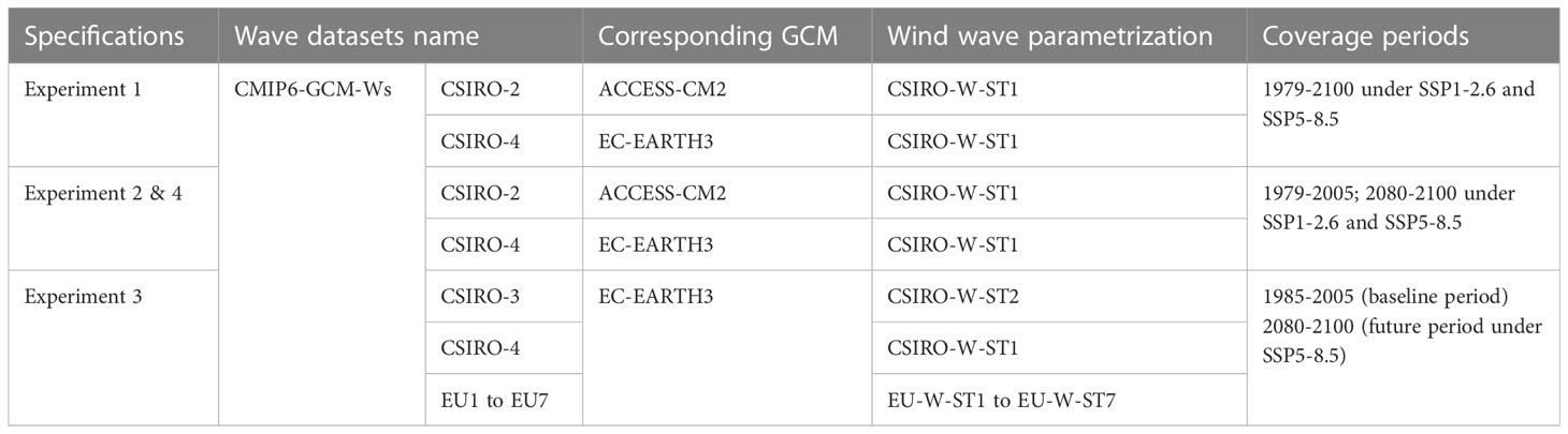
Table 1 Wave datasets used for each experiment.

To rank the reliability of GCMs’ outputs, the GCMs’ performance to properly reproduce historical patterns was first evaluated against the CAWCR 24 min resolution wave hindcast (Center for Australian Weather and Climate Research, Smith et al., 2020). This hindcast has been shown to have good accuracy compared to in situ wave measurements within this region (i.e., Brisbane wave buoy data for the period 2000 to 2020; Zarifsanayei et al., 2022a). For the comparison of GCM-Ws with the reference dataset, wave roses and plots of the average wave energy flux per direction were considered (refer to section results and discussion). To quantify the performance, the following metrics were adopted:

a) Bias

$\begin{array}{ll}Bia{s}_j=\frac{1}{N}{\displaystyle {\sum }_{i=1}^{N}GCM{W}_j}-\frac{1}{N}{\displaystyle {\sum }_{i=1}^{N}REF}& (1)\end{array}$

Where j is the GCM-W number, N is the length of the timeseries, i is the index of the data, REF is the reference hindcast dataset (i.e., CAWCR 24 min).

b) PDF-Score (Soares and Cardoso, 2018; Lima et al., 2019) which finds the minimum common area between two empirical probability density functions (PDFs), of the reference data and each of the GCMs, respectively, yielding values between 0 (no matching) to 1 (perfect match, i.e., same PDF).

$\begin{array}{ll}PDFScor{e}_j=\int \text{min}(PD{F}_{GCM{W}_j},PD{F}_{REF})& (2)\end{array}$

c) M-Score (Semedo et al., 2018) which is a non-dimensional measure, ranging from a hypothetic zero (no skill) to a maximum of 1000 (perfect skill).

$\begin{array}{ll}MScor{e}_j=\frac{2}{\pi }\arcsin \left(1-\frac{MSE}{V_{GCM{W}_j}+V_{REF}+{(M_{GCM{W}_i}+M_{REF})}^2}\right)\ast 100& (3)\end{array}$

Where MSE, V and M stands for mean square error, variance and mean, respectively. As GCM-Ws are not time constrained to the reference data, all inputs of the M-Score formula are multi-year monthly means of H_s, T_p, and D_m.

d) Yule-Kendall skewness coefficient (Ferro et al., 2005) gives information on the skewness of GCM-Ws distributions in comparison with reference forcing. The closer this coefficient is to zero, the more similar GCM-W is to the benchmark/reference data.

$\begin{array}{ll}Y{K}_i={\left[\frac{(P_{95}-P_{50})-(P_{50}-P_5)}{(P_{95}-P_5)}\right]}_{GCM{W}_j}-{\left[\frac{(P_{95}-P_{50})-(P_{50}-P_5)}{(P_{95}-P_5)}\right]}_{REF}& (4)\end{array}$

Where P₅, P₅₀, P₉₅ refer to the relative position of 5^th, 50^th, 95^th quantiles, respectively.

The Bias was calculated for all wave parameters, the PDF score was applied only to parameter H_s, and YK coefficient was calculated for the parameters H_s and T_p. The M-Score metric was calculated for all wave parameters condensed into multi-year monthly means.

The capability of GCM-Ws to reproduce the patterns of waves for the historical period is an important factor to evaluate their reliability. GCM-Ws may contain significant biases with respect to observational/reference datasets, mainly inherited from the GCMs’ simulations conducted by different approaches for parametrizations of climate processes (Morim et al., 2018). To reduce the systematic errors in GCM-Ws, choosing a reference dataset and applying bias correction is a common approach (e.g., Lemos et al., 2020a, Lemos et al., 2020b). The correction methods are time-independent, modifying the general patterns of wave parameters represented in each quantile (statistical distribution). It has also been shown that applying bias correction techniques to offshore wave forcing conditions (i.e., GCM-Ws) is necessary to capture reasonable patterns for nearshore wave and sediment transport during the baseline period (Zarifsanayei et al., 2022b). Moreover, it was shown that the bias-corrected forcings preserve the signals of climate change presented by the original forcings. Hence, following Zarifsanayei et al. (2022b), using the CAWCR wave hindcast as the reference, the correction approaches of Empirical Quantile Mapping (EQM) for parameter D_m, and Empirical Gumbel Quantile Mapping (EGQM) for parameters H_s and T_p were employed to correct systematic errors of all offshore forcing conditions used in this study (Table 1).

2.3 Projected nearshore waves and response of sediment transport models

To significantly decrease the large computational costs of wave transformation into the nearshore, wave transfer functions were developed following Antolínez et al (Antolı́nez et al., 2016; Antolı́nez et al., 2018). Generally, the functions require offshore wave samples covering the entire parameter range of the datasets, a calibrated spectral wave model to transfer the samples to nearshore, and an algorithm for reconstruction of the whole time series of nearshore waves (i.e., development of wave transfer functions). The algorithm captures the non-linear relationships between offshore and nearshore waves represented by the wave samples. In total, three types of wave transfer functions were developed by which the nearshore waves for each site were reconstructed. Figure 4 outlines the steps followed to generate the transfer functions.

FIGURE 4

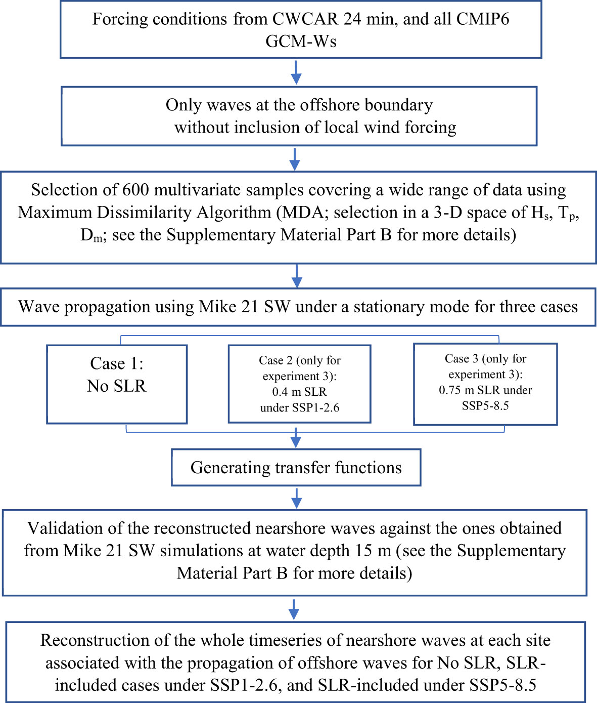
Figure 4 Flow chart of nearshore wave reconstruction.

The spectral wave model employed in this study, was Mike 21 SW (DHI, 2017) which was previously developed and calibrated for the study site by Zarifsanayei et al. (2022a). Samples of the bias corrected offshore wave parameters H_S, T_p, D_m were utilized for the offshore boundary condition of a spectral wave model (i.e., Mike 21 SW; DHI, 2017) to transfer offshore waves of GC to the nearshore sites. The wave parameters were converted to wave spectra whose frequency and directional spaces complied with a JONSWAP distribution (with a peak enhancement factor 3.3) and cosⁿ distribution, respectively. No local wind forcing was considered for wave transformation, as the spatial resolution of the GCMs used in this study was not sufficient to capture the local wind patterns properly (for further details on the effect of local wind on wave transformation refer to Zarifsanayei et al., 2022a).

To generate transfer functions for the SLR experiment, it was assumed that the shape of the coastal profiles from the dry beach out to a the depth of closure (~ 15 m) remained constant meaning that the relative water depth within the active profile remains unchanged in response to SLR. This assumption aligns with the current coastal management strategy of the GC to compensate for any sediment deficit by the placement of sand locally as well as the operation of sand by-passing/back-passing systems in the south and north of Gold Coast. SLR values averaged over the far future period (2080-2100) under SSP1-2.6 and SSP5-8.5 were extracted from the NASA sea level projection tool developed for IPCC AR6 (IPCC, 2021) for the nearest output grid point to GC (see Supplementary Material, Part B for more details). The averaged SLR values were applied in a stationary form in the wave model (i.e., assumed to be constant over time; 40 cm under SSP1-2.6 and 80 cm under SSP5-8.5). In all simulations, waves were extracted at the same water depth (i.e., 15 m). However, due to SLR the position of wave data extraction was shifted toward the coast (~ 50 m under SSP1-2.6 & 100 m under SSP5-8.5). Shifts in the position of wave data extraction for SLR inclusion cases can roughly mimic the SLR impacts on the patterns of wave dissipation and the resulting wave-driven sediment transport.

The reconstructed nearshore waves at water depth 15 m, for historical and future periods were transferred within active zone of coastal profiles (i.e., less than 15 m depth) using the widely used wave transformation methods (Battjes and Stive, 1985; Larson et al., 2010), and the breaker index of Kamphuis (2010). Afterwards, the transformed waves were introduced into the LST models previously calibrated for hindcasting LST patterns along the GC shoreline (more details can be found in Zarifsanayei et al., 2022a). Two classes of LST models, including simplified (bulk formula) models (i.e., van Rijn, 2014; modified CERC and Kamphuis, Mil-Homens et al., 2013; Shaeri et al., 2020) and process-based models (i.e., DHI-LITPACK with four different set- ups, Kristensen et al., 2016) were used to capture a wide range of sediment transport model uncertainty and its interaction with forcing conditions.

The setup of the LST models is described in detail by (Zarifsanayei et al., 2022a) but for ease of reference a brief overview is provided here. The models were set up according to the available data at the study area including: sediment properties; an average barred beach profile using the model of Holman et al. (2014) fit to beach profiles measured since 1966; shoreline orientation from historical surveys and post-processed satellite images; and hourly wave forcing obtained from a nearshore wave rider buoy located at north Gold Coast. The models underwent extensive sensitivity analysis before being calibrated with the forcings obtained from the nearshore wave buoy at North Gold Coast, and the annual LST rates estimated from observations and sand bypassing system operation at North Gold Coast for the period of 2007 to 2020. Note that all settings of the calibrated models (e.g., beach profiles, shoreline orientation, sediment size, etc.) remained unchanged for the LST projections of this study. Morphological changes to the profiles were not considered as it is assumed that, for the Gold Coast shoreline, no changes in sediment sources and sinks will occur due to the current management strategies aimed at maintaining the shoreline stability. In all simulations, the temporal resolution of LST models was the same as the temporal resolution of the time series of the forcing conditions used. No lateral boundary conditions were required for the LST models because the focus of this paper was only on projecting the future patterns of potential LST rates, not on coastal evolution or shoreline change. Additionally, the response of LST models to the nearshore waves associated with CAWCR 24 min resolution offshore data was considered as the reference LST along the coast.

2.4 Uncertainty analysis

For each experiment and site, the total uncertainty was obtained by an ensemble that consists of wave forcing datasets projected under one/two scenarios, and different sediment transport models. Following Hawkins and Sutton (2010), to narrow the range of the uncertainty in ensemble modelling a simple weighting scheme was also adopted. The weighting scheme was based on two criteria:

a) The difference between annual mean LST pattern along the coast represented by each ensemble member and the reference LST; and

b) Shoreline orientation along the coast (represented by each ensemble member) for which mean net annual LST tends to zero and its difference to that of the reference LST.

The two criteria above were translated into Euclidean distances by which a weight was calculated and allocated to each ensemble member individually. More details on this approach can be found in Zarifsanayei et al. (2022b).

Another important task of uncertainty analysis is detecting the trends of changes among noisy projected values using the continuous time series. The modified Mann-Kendall test (that accounts for autocorrelation of the time series) was used (Hamed and Ramachandra Rao, 1998). To implement the modified Mann-Kendall test for experiment #1, the 3-hourly continuous timeseries of LST rates were converted to seasonal and annual quantities which were then smoothed over annual (seasonal quantities) and decadal (annual quantities) time scales. The total uncertainty of LST projections was then decomposed following Hawkins and Sutton (2009) to establish the uncertainty associated with emissions scenario, model and internal variability of the Earth-climate system (cf. Supplementary Material, Part C for details). For experiment #2 which utilised block time sliced timeseries of waves (for the far future), the projected changes in the LST patterns were decomposed into the predefined sources (scenarios, GCMs, LST model, and non-linear interactions) using an ANOVA subsampling technique and then compared with the uncertainty contributions previously found for CMIP5-Ws-driven LST patterns (Zarifsanayei et al., 2022b).

3 Results and discussion

3.1 Evaluation of GCM-Ws

Figure 5 shows the annual mean wave energy flux (WEF) on a polar coordinate system for each of the CMIP6 GCM-Ws in comparison with the CAWCR reference hindcast. In addition, wave roses are provided in Supplementary Material, Part A. Overall, the CMIP6 GCM-Ws are unable to accurately reproduce the reference data (i.e. the predominant S to SE directions). In particular, the EU1-, EU7- and CSIRO-2-driven waves show the greatest errors in wave energy patterns predicting the predominant wave direction to be from the east (Figure 5A). Some of the wave datasets, such as EU-2 and EU-5, fail to predict the energy magnitude due to large biases in H_s. Notably, all the EU wave simulations which use the same wind forcing (EC-EARTH3) but with different parameterization schemes, indicate large discrepancies which should challenge the practice of relying only on a single wave model and/or parameterization for projection studies.

FIGURE 5

Figure 5 Wave energy flux patterns presented by CMIP6-Ws. (A) original data, (B) bias corrected data at locations P2 and P3.

Compared to CMIP5-Ws (Zarifsanayei et al., 2022b), the global wave models used for the CMIP6-Ws have a higher spatial resolution (~ 0.5-0.7 deg vs ~ 1 deg res). However, still large biases relative to the reference forcing are observed (Figure 5A). Nonetheless, noting that the CSIRO 2-Ws CMIP6 dataset is the closest to the ACCESS-1.0-Ws in the CMIP5 dataset in terms of model configuration, it seems that CSIRO CMIP6 wave projections have improved performance, particularly for parameters H_s and D_m (~ 0.3 m & 6 degrees decrease in biases respectively; see Supplementary Material, Part A). Although the ACCESS-CM2 (CMIP6) and ACCESS1.0 (CMIP5) GCMs have the same horizontal resolutions, the number of vertical layers in the CMIP6 run was 85 layers compared to 35 in CMIP5 which leads to better performance (Bi et al., 2020). Despite the increase in spatial resolution of CMIP6 GCMs, they still remain too coarse to resolve sea surface local wind/sea breeze patterns.

It is important to note that the significant errors in GCM-Ws are not limited to this study site (Gold Coast). In fact, GCM-Ws based on global wind (and sea ice concentration) fields, are generally unable to accurately represent most small-scale, local-to-regional phenomena. Therefore, bias correction procedures are important to improve the accuracy of the wave datasets near the coast which adjust GCM-W outputs towards reference hindcast datasets that are usually of higher resolution and/or based on observations. For this particular case study, while there may be several reasons for the misrepresentation of wave energy flux patterns, it’s believed that a significant portion of the errors can be attributed to horizontal resolution and even land-sea masks (Meucci et al., 2022). This means that GCM-Ws could represent wave patterns at regional and local scales if the appropriate resolution, bathymetry, and land-sea mask are provided. Due to the poor performance of the original GCM-Ws at the site, the bias correction procedure is necessary, not to introduce new physical processes, but to incorporate observational features that are too local to be accurately captured by the original GCM-Ws. Moreover, these limitations should remain consistent over time because no changes in resolution, bathymetry, or land-sea masks were made during the wave climate projections. Therefore, a consistent bias correction method is considered capable of providing a realistic projection of the future wave climate with a low risk of manipulating the signals of climate change presented by the original wave datasets (for more discussion on this matter see Zarifsanayei et al., 2022b).

Figure 5B shows the GCM to reference comparison after bias correction of the CMIP6-Ws which, as expected, now show essentially the same patterns to the reference long-term annual wave energy flux approaching the Gold Coast region. That is, after bias correction, the original GCM-Ws waves now correctly demonstrate the predominant S to SE directions rather than from the E (see Supplementary Material, Part A).

Figure 6 shows that original (uncorrected) CMIP6-Ws datasets have biases in the range of –0.6 to +0.4 m for H_s, –2 to 2 s for T_p and -5 to -20 degrees for D_m. The wave datasets associated with EU1, EU2 and EU7 exhibit the greatest errors across almost all wave parameters. Such large biases in forcing conditions during the historical period, particularly for parameter D_m, can lead to remarkable errors in projection of wave-driven sediment transport and coastal evolution patterns. After bias correction, consistent improvement of all the accuracy metrics for all GCM-Ws is seen (also see Supplementary Material, Part A for PDF-score). Another important point to consider is that bias correction approaches may not be capable of fully resolving all systematic errors in GCM-Ws datasets, (e.g., signals of climate change), particularly if the original datasets exhibit quite large biases in wave direction patterns (e.g., EU1- & EU5-driven waves).

FIGURE 6

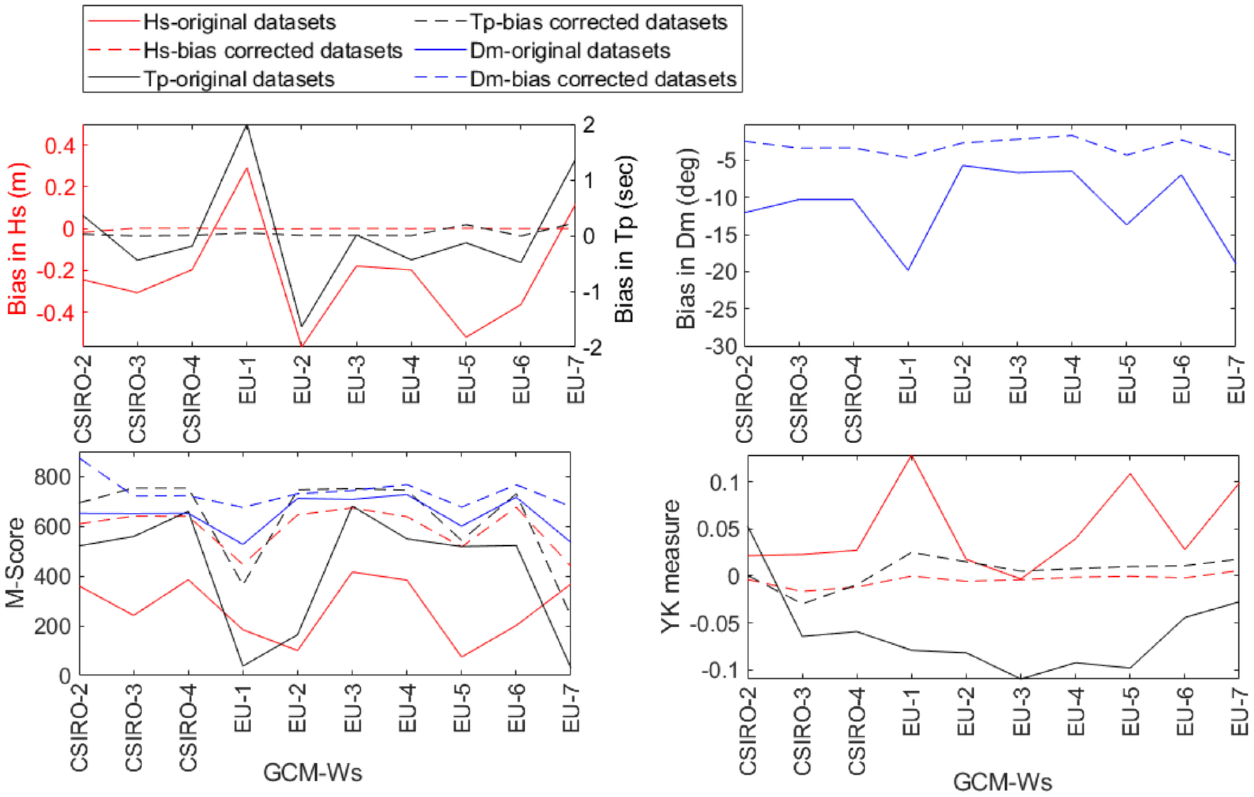
Figure 6 Metrics to evaluate the performance of CMIP6-Ws before and after bias correction; Negative values for D_m indicate anti-clockwise deviation.

Comparing the signals of wave climate change (on a monthly scale) for the far future, under the worst-case scenario associated with CSIRO-CMIP6-Ws (SSP5-8.5), with those of CSIRO-CMIP5-Ws (RCP8.5), a consensus on the rotation of waves toward east direction is found. This is particularly evident during the period of June to October (on average, 12 degrees anti-clockwise rotation, see Supplementary Material, Part A). Under SSP1, on average CSIRO-CMIP6-Ws, indicate a projected decrease in H_s of 5% and a 7 degrees rotation towards the east. It is noted that the number of GCMs in the CSIRO-CMIP6 wave simulations is presently limited to 2, as compared to 8 for the CSIRO-CMIP5 ensemble, and therefore currently has limited ability to accurately capture the uncertainty associated with GCM selection.

Amongst the ensemble of wave model parameterization schemes (i.e., CSIRO-3 &4, EU1 to EU7), there is generally a consensus on the sign of changes (increase or decrease) in wave parameters but significant differences in the magnitude of the projected changes exists for all wave parameters (see Supplementary Material, Part A). For instance, from June to October, the difference in the projected changes in monthly mean D_m reaches up to 8 degrees. As shown by Kumar et al. (2022) and Lobeto et al. (2023) at other regions around the world, the effect of wind-wave parametrizations on wave simulation outputs can be so large that it leads to no consensus on either magnitude or the sign of change, possibly hiding the signals of wave climate change. Such discrepancies can not only jeopardise the robustness of offshore wave projections conducted by dynamical approaches, but also have great implications for statistical wave projections where usually reference forcing is needed to train wind-wave/weather type transfer functions (e.g., Camus et al., 2017). The reference forcing is usually obtained from the output of only one dynamic-based wave hindcasting project (e.g., ERA5; Hersbach et al., 2020), while an ensemble of wave hindcasting simulations is required (Morim et al., 2022).

3.2 LST projections, experiment #1

One of the main advantages of the new CSIRO-CMIP6 wave datasets is the archiving of the long-term (> 100 years) continuous time series. Continuous time series of waves better depict long-term, natural climate variability (e.g. Odériz et al., 2021). The natural variability in wave climate will flow through in to the nearshore wave forcing and resulting sediment transport patterns, making the detection of climate change signals challenging. Hence, experiment #1 was designed to examine this issue. As previously illustrated in Figures 1, 4, the entire timeseries of offshore waves were translated into 3-hourly timeseries of LST rates at each site. The LST timeseries were then converted to seasonal, and annual LST rates and smoothed within annual and decadal time windows respectively. For each site, linear trends were fitted to the mean of each of the seasonal and annual LST rates, and the significance of the trends checked with the modified Mann-Kendall approach.

The results for site D (located in the middle of the Gold Coast coastline, see Supplementary Material, Part D) indicate that, at the seasonal scale, the smoothed net LST rates presented by CSIRO-CMIP6 wave datasets fluctuate between 65,000 m³/season and 230,000 m³/season. Generally, the mean and standard deviation of seasonal smoothed LST rates are both approximately 140,000 m³ (i.e. coefficient of variation ~ 1) which suggests significant natural variability data and likely weak signals/trends on the seasonal scale. Additionally, although the seasonal LST patterns obtained from CSIRO2-Ws are relatively consistent with those obtained from reference forcing, using CSIRO4-Ws does not lead to very promising LST patterns for the same period (see violin plots for LST rates in Supplementary Material, Part D). For the SSP1-2.6 scenario, both CSIRO2-Ws and CSIRO4-Ws project decreasing trends for net LST rates whereas under SSP5-8.5, CSIRO2-Ws and CSIRO4-Ws project a decreasing and increasing trends for seasonal LST rates respectively. After applying the modified Mann Kendall test to the seasonal LST rates, the observed seasonal trends are found to insignificant (see Supplementary Material, Part D).

On the annual scale (see Figure 7), the smoothed net LST rates presented by CSIRO-CMIP6 wave datasets fluctuate between 450,000 m³/year and 680,000 m³/year. The mean and standard deviation of the smoothed annual LST rates are 530,000 m³/year and 120,000 m³/year, respectively (coefficient of variation ~ 23%). The annual trends were found to be significant for all cases however the trends associated with CSIRO2-Ws and CSIRO4-Ws under SSP5-8.5 are not consistent (first one is negative and the second one is positive). It seems that the trends are highly influenced by the LST rates during the last three decades (i.e., 2070-2100), where the CSIRO4-SSP5 shows a strong increase during this period which is not seen for CSIRO2-SSP5. This highlights the significant uncertainty associated with far future projections.

FIGURE 7

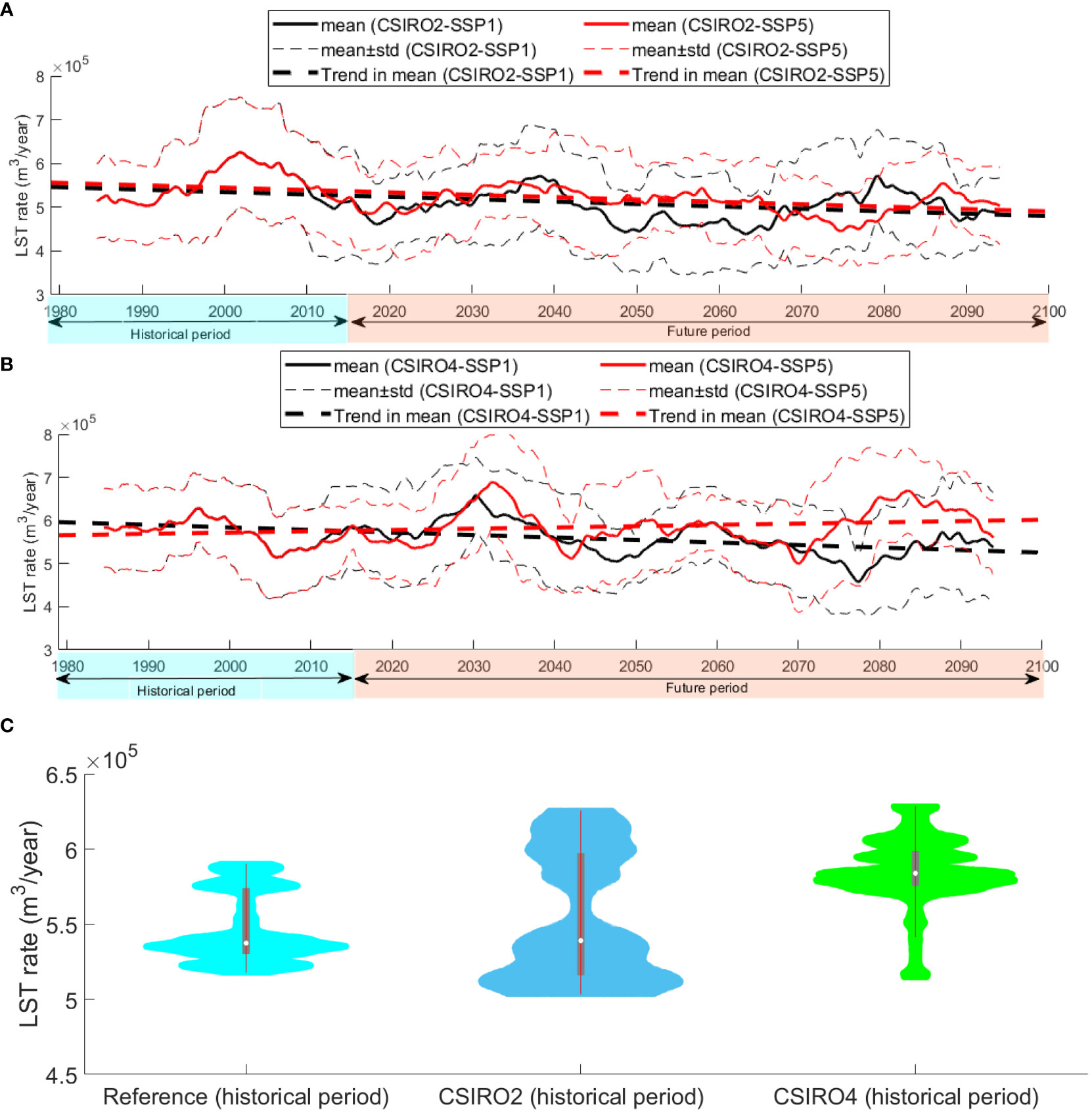
Figure 7 Smoothed annual net LST rates at site D associated with (A) CSIRO2-Ws and (B) CSIRO4-Ws under SSP1 and SSP5; (C) Violin plots of the response of all LST modes to the datasets of CAWCR 24 min resolution (Reference), CSIRO2-Ws and CSIRO4-Ws for historical period; all LST models were used for these plots; The violin plot shaded area is the approximation of the probability density function (PDF) through a kernel density estimation, while the remaining information corresponds with that of a boxplot.

Noteworthy points can be perceived from smoothed annual LST patterns. Firstly, the smoothed signal is periodic in nature with a period of ~20 to 30 years which suggest significant inter-decadal natural climate variability (i.e., combination of variability of earth-climate systems in the presence and absence of external forcing; IPCC, 2021). This finding suggests that using block time slice averaging (e.g. far future from 2080-2100) to estimate projected changes in sediment transport rates/coastal evolution could lead to erroneous outcomes because of the significant natural variability. For example, if one decides to employ CSIRO2-Ws under SSP1-2.6 and SSP5-8.5 for the period 2020 to 2040, they might conclude that global warming yields increasing LST rates, while the long-terms trends of LST rates for CSIRO2-Ws-SSP1-2.6 and CSIRO2-Ws-SSP5-8.5 are negative and positive, respectively. Secondly, the importance of model selection (i.e., both GCM-Ws, large source of uncertainty and LST models, less uncertainty; Zarifsanayei et al., 2022b) seems to be significant for both the near future (e.g., 2030-2050) and the far future (2080-2100). Additionally, scenario uncertainty becomes increasingly significant for LST projections after 2050.

These points have vital implications for coastal management planning, where the time horizon of projects should first be clearly defined, and then according to that, uncertainty sampling (i.e., incorporating sources of uncertainty within the modelling chains) should be conducted properly to inform the decision-makers about the range of uncertainty. Continuous time series of wave-driven sediment transport patterns provide the opportunity for coastal planners to estimate the contribution of internal variability, model, and scenario uncertainty to the total uncertainty of sediment transport projections. The results of uncertainty decomposition (see Figure 8) clearly show that for near-future planning, a large part of uncertainty arises from model selection and natural variability of the system (i.e., for the period 2030-2050 on average, 4% scenario, 57% model, and 39% internal variability). To reduce model uncertainty, significant effort in future works should continue to be directed towards understanding the earth-atmospheric system and improving models, particularly GCMs. While the importance of natural variability decreases significantly in time and the fraction of total model uncertainty slightly decreases in time, the fraction of uncertainty due to assumed emissions scenario increases dramatically. For the far future, on average for all sites, 25% scenario, 54% model and 21% internal variability contribute to total uncertainty. Note that isolation of the natural variability in projected LST rates was based on the underlying assumption that climate change is captured by a linear trend as assumed in other sediment transport studies (Splinter et al., 2012; Chowdhury and Behera, 2017; Başaran and Arı Güner, 2021).

FIGURE 8

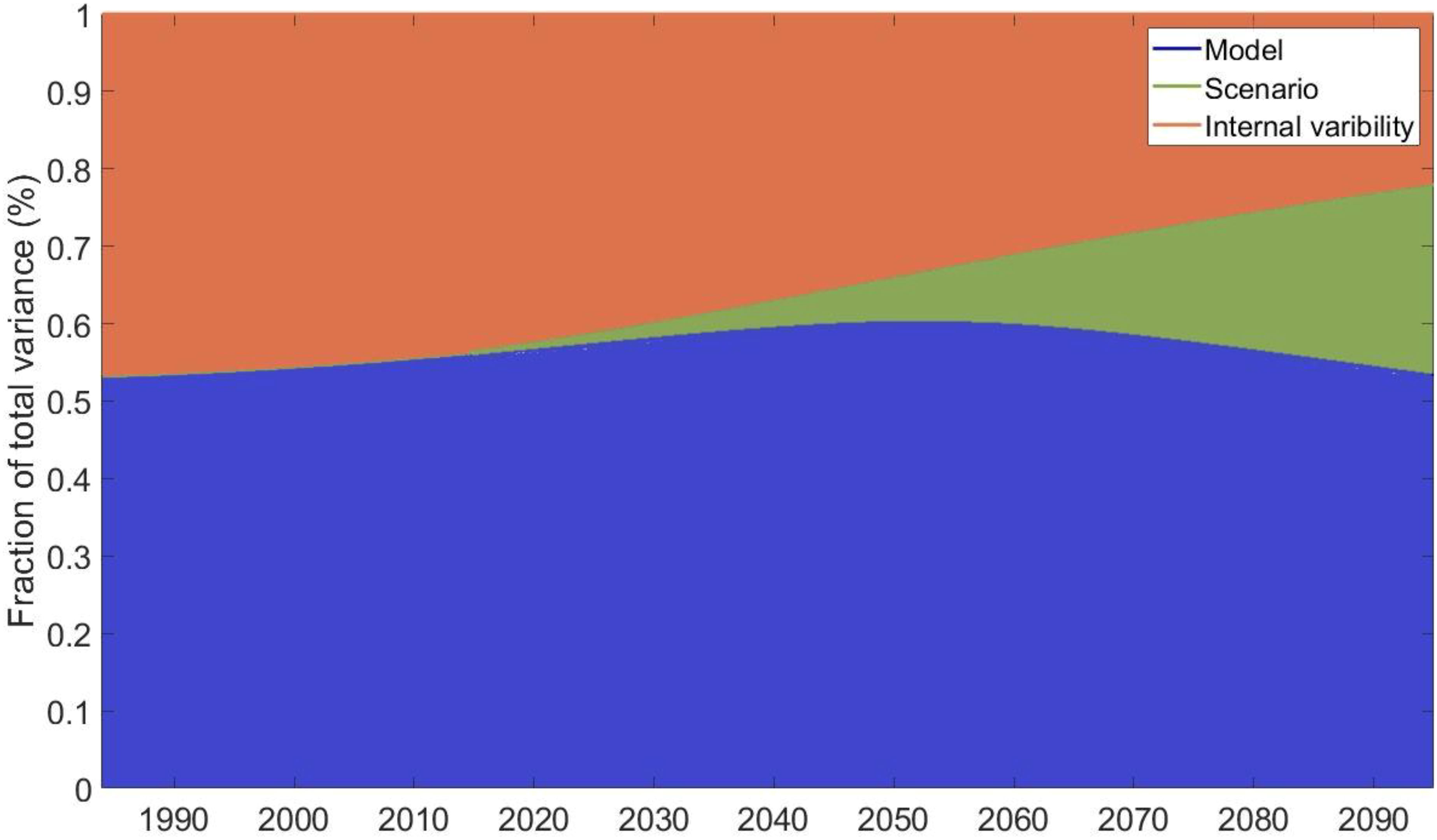
Figure 8 Decomposition of total uncertainty into model, scenario and internal variability; averaged over all sites.

3.3 LST projections, experiment # 2

To compare the CSIRO-CMIP6-Ws driven LST patterns and the corresponding uncertainty with those of CSIRO-CMIP5-Ws (Zarifsanayei et al., 2022b), sliced time series of LST rates for both baseline and the far future periods (1979-2005 and 2080-2100) for all sites were analysed. For the historical period, the annual mean LST rates associated with the ensemble are consistent with those of the reference, showing a good performance of bias correction and weighting schemes that were applied to decrease the errors in the projection of LST patterns (see Supplementary Material, Part D). Under SSP1-2.6 and SSP-5-8.5, the ensemble mean projects 7% and 9% decreases in net annual mean LST rates, respectively (see Figure 9). The decrease in the LST rates along the coast, and the predominance of net northward LST rates under both scenarios are in agreement with the CMIP5 findings of Zarifsanayei et al. (2022b). Note that CSIRO-CMIP5-Ws datasets were projected under one middle scenario (RCP4.5) and a pessimistic scenario (RCP8.5), while CSIRO-CMIP6-Ws datasets sampled uncertainty from an optimistic (SSP1-2.6) and a pessimistic scenario (SSP5-8.5). That is why the range of uncertainty in LST projections under SSP5-8.5 is significantly larger than that of SSP1-2.6 (as depicted by the highlighted areas in Figure 9A in comparison with Figure 9B).

FIGURE 9

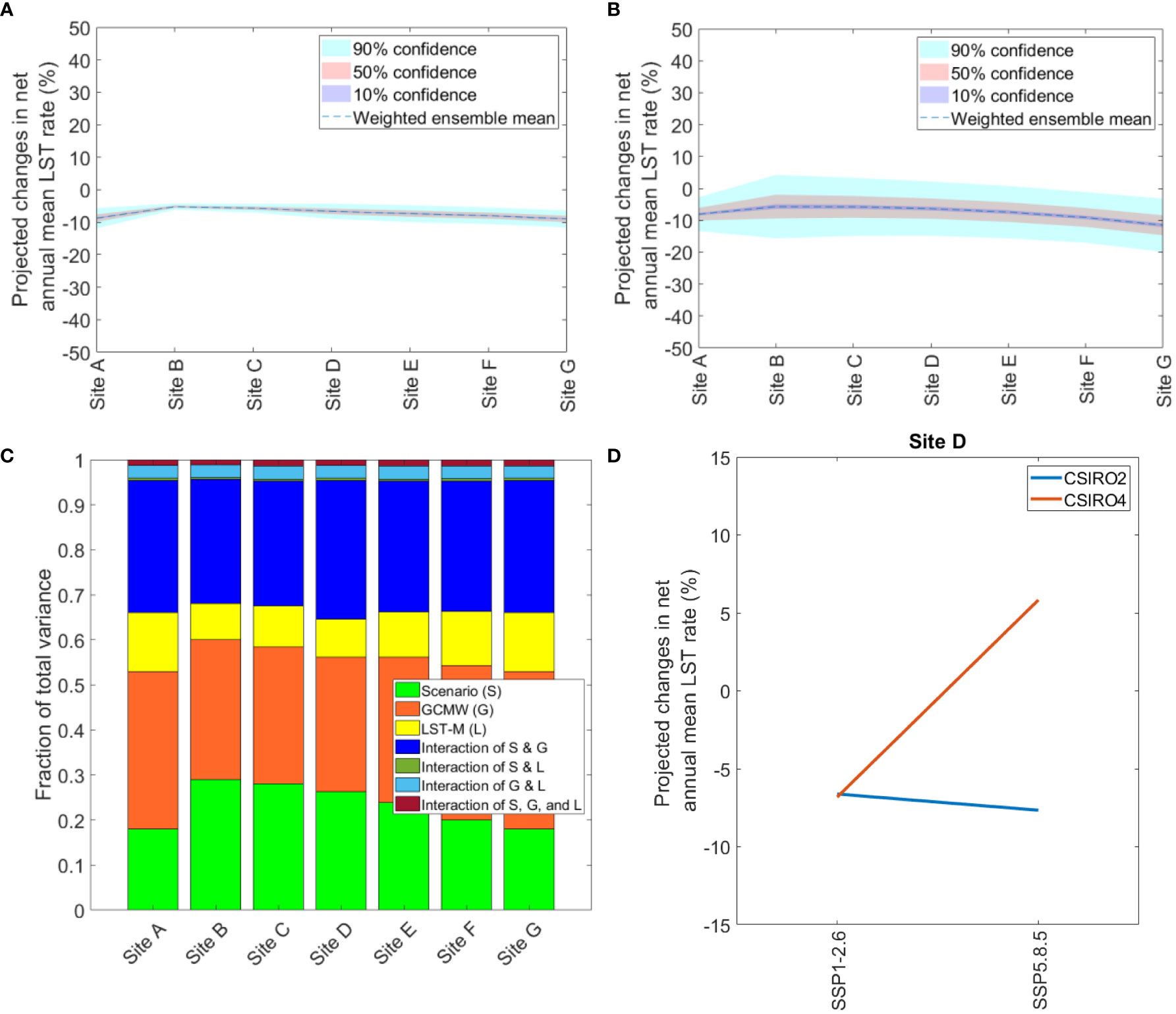
Figure 9 Uncertainty analysis for sliced timeseries of waves for far future period 2080-2100; projected changes in annual mean LST rates (A) under SSP1-2.6 and (B) under SSP5-8.5, (C) uncertainty contributions obtained from ANOVA, (D) interaction of GCM-Ws and scenarios to project LST rates at site D.

Seasonal LST rates (Supplementary Material Part D) indicate that a large fraction of the annual net LST rate occurs during summer and then winter (particularly during March, April and May). The ensemble mean projects that the net LST rates decrease during these seasons (5% to 10% (10% to 20%) during summer (winter), under SSP1-2.6 and SSP5-8.5, respectively). During spring, significant (relative) changes in LST rates are projected but note that significantly less LST occurs during spring compared to the other seasons and so the corresponding absolute changes have an insignificant influence on annual LST projections (detailed graphs on the projected changes in seasonal northward and southward LST rates can be found in Supplementary Material Part D).

The ANOVA results (Figure 9C) imply that, on average, scenario uncertainty contributes to 23% of total uncertainty, which is larger than previous findings for CMIP5 (16% for scenario uncertainty; Zarifsanayei et al., 2022b). The contributions of GCM-Ws and LST model uncertainty to total uncertainty are 30% and 10%, respectively. Compared to previous findings for CMIP5 (~ 35% for GCM-Ws uncertainty; Zarifsanayei et al., 2022b), slight decrease (~ 5% decrease) in contribution of GCM-Ws to total uncertainty, is observed. Nonlinear interaction of GCM-Ws and scenario is also significant (24%, see Figures 9C, D), questioning the reliability of LST projections based on a single emission scenario (e.g., Chowdhury et al., 2020; Fernández-Fernández et al., 2020).

3.4 LST projections, experiment # 3

In experiment #3, an ensemble of wave projections, generated under different parameterizations, was employed to project LST rates. To determine the importance of this source of uncertainty, the results of LST rates obtained from the full ensemble forcing (CSIRO3 and 4 plus EU1 to EU7) were compared with those of the subset of ensemble forcing CSIRO-3 and 4 in terms of intra- and inter-annual variabilities (see Figures 10A, B for site D). Such discrepancies can increase the range of uncertainty in the LST projections (as shown in Figures 10C, D) and, at the same time, can impact the robustness of the projections as the standard deviation of the ensemble gets larger than the ensemble mean. As wave model parameterizations also have an impact on the distribution of wave driven LST rates (see violin plots in Supplementary Material, Part D) then will also flow on to increased uncertainty in the projection of erosion and recovery periods of the coast (e.g., Antolínez et al., 2018; Toimil et al., 2022). Note that compared to the other sites, a larger level of uncertainty in the LST projections for site A is observed. This is likely due to the fact that the nearshore bathymetry in this area is more complex (reefs and headlands) and as such more complicated refraction patterns result.

FIGURE 10

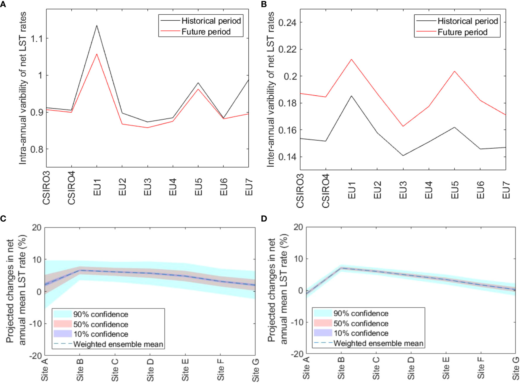
Figure 10 Implications of wind-wave parameterization uncertainty for LST projections; (A) Intra-annual variability (i.e., standard deviation of the monthly means/time slice mean) of net LST rates at site D; (B) Inter-annual variability (i.e., standard deviation of the annual means/time slice mean) of net LST rates at site D; (C) LST projections associated with the ensemble forcing CSIRO 3 &4 and EU1-EU7; (D) LST projections associated with the ensemble forcing CSIRO 3 & 4.

3.5 LST projections, experiment # 4

Experiment #4 examined the influence of SLR on LST projections based on sliced timeseries of CSIRO-3 and 4 for the far future under SLRs corresponding to SSP1-2.6 and SSP5-8.5. In essence, the effect of SLR on wave transformation depends on the characteristics of the lower shoreface and shelf, and how wave dissipation due to bottom friction, wave refraction and shoaling takes place. The results imply that the inclusion of SLR in wave transformation, under SSP1-2.6, yields only meagre changes in the LST projections (~ -0.5%), compared to the case of no-SLR (compare Figure 11A with Figure 9A). This is due to the small value of the projected SLR under SSP1-2.6 (i.e., 0.4 m) that does not have a significant influence on wave transformation. Under SSP5-8.5, the inclusion of SLR leads to a larger decrease in the projected rates of LST (~ -2%), compared to the case of no SLR, indicating that in this case the offshore waves are slightly more dissipated (compare Figure 11B with Figure 9B).

FIGURE 11

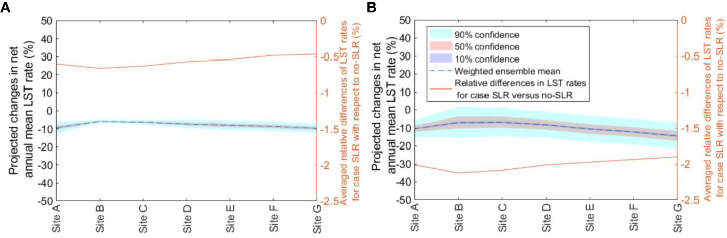
Figure 11 Projected changes in annual mean LST rates for case SLR inclusion, under (A) SSP1-2.6 and (B) SSP5-8.5.

4 Limitations and the way forward

Although efforts were made in this study to shed light on some aspects of uncertainty in the LST projections, still many other experiments are recommended for future work.

First, as shown, continuous time series of waves are required to reveal climate variability patterns and their implications for coastal studies. However, only a limited number of projected offshore wave datasets covering a continuous long-period are currently available (e.g., CSIRO CMIP6-Ws for two GCMs). Ideally, a larger number of GCMs for each scenario/pathway are required to understand how much the wave-driven sediment transport projections are consistent with each other and to better resolve the significant uncertainty associated with GCM and scenario selection (e.g., Lehner et al., 2020). In this regard, using statistical wave downscaling rather than dynamical wave simulations is preferred to consider a large number of GCMs (e.g., 50 GCMs) for wave projections. However, as the findings of this research showed, the reference forcing required for statistical downscaling is impacted by wind-wave parametrizations, using more than one reference forcing dataset (an ensemble) is also recommended.

Secondly, the spatial resolution of GCMs (e.g., 0.5-3 deg) is too coarse to resolve local scale wind fields and so finer-scale climate models are needed for this purpose. The impact of local wind on wave transformation, as shown by Zarifsanayei et al. (2022a), may increase the uncertainty in LST calculations. In this study, wave parameters associated with total wave energy were used as the offshore boundary condition of a wave transfer function. For future works, working with directional spectral boundary conditions and transferring them to the nearshore zone is also recommended. In this regard, bias correction of spectral data at the offshore boundary of a wave model, transferring offshore forcing, and reconstruction of the nearshore spectra are very challenging goals.

Another challenge is that, even if nearshore spectra are projected properly, the current LST models used in this study, only work with integrated wave parameters rather than full spectral data. This implies that the nearshore spectrum should be converted to integral parameters again, increasing the errors in LST projections, particularly in the case of prevalent multi-modal nearshore spectra. Hence, development of a new generation of computationally efficient, wave spectra driven LST models is encouraged.

The present study examined the effect of SLR on wave transformation and hence LST projections under the assumption of a fixed profile shape such that the relative water depth from the beach to 15m depth remained unchanged. Whilst this assumption aligns with the current coastal protection policy of the City of Gold Coast to preserve coastal profiles by beach nourishment, using more sophisticated approaches in the literature to update the upper and lower shoreface profiles in response to SLR (e.g., McCarroll et al., 2021) is suggested for future research.

Finally, for potential future work, it could be valuable to apply additional bias correction methods (e.g., multivariate bias correction or correction of the full wave energy spectrum) and compare their results to the univariate approach used in this study.

5 Summary and conclusions

Four experiments were conducted for seven sites along the Gold Coast shoreline to investigate uncertainty sources in LST projections due to: (1) working with continuous time series of wave forcing (experiment #1); (2) CMIP experiment family based on sliced time series of waves from CSIRO-CMIP6-Ws and CSIRO-CMIP5-Ws (experiment #2); (3) wave-model parametrizations to generate wave projections (experiment #3); and (4) the influence of SLR on regional wave transformation (experiment #4). For each experiment, a separate weighted ensemble consisting of offshore wave forcing conditions, a hybrid wave transformation method and eight LST models were used.

The results of experiment #1 indicated that the annual LST rates obtained from continuous time series of waves were subject to the influence of inter-decadal climate variability acting on timescales of 20-30 years. Such findings imply that LST projections based on sliced time series of waves (which do not capture inter-decadal natural variability), would be prone to unreliable conclusions about the impacts of climate change on LST.

The results of uncertainty decomposition clearly show that for near-future coastal planning, a large part of uncertainty arises from model selection and natural variability of the system (e.g., for period 2030-2050 on average, 4% scenario, 57% model, and 39% internal variability). While the influence of natural variability decreases significantly over time, model uncertainty only slightly decreases in time and scenario uncertainty increases dramatically. Considering the far future, averaged over all sites, 25% scenario, 54% model and 21% internal variability contribute to total uncertainty.

In experiment #2, sliced time series of waves (for the far future) were used to facilitate a comparison of LST projections between CSIRO-CMIP6-Ws and CSIRO-CMIP5-Ws. The results showed that CSIRO-CMIP6-Ws driven LST projections are broadly similar to their CMIP5 counterparts, namely decreasing LST rates along the coast and net northward LST rates. However, due to different definitions of emission scenarios adopted in AR6 compared to AR5, the range of uncertainty in the LST projections due to scenario selection increased. On average, uncertainty of the projected changes in the LST rates is controlled by scenario (23% of total uncertainty), GCM-Ws (30% of total uncertainty), LST model (10% total uncertainty), non-linear interaction of GCM-Ws and scenario (24%), and other nonlinear interactions (3%). Compared to the previous findings for CMIP5 (Zarifsanayei et al., 2022b), a slight increase (~7% increase) was observed in the contribution of scenarios uncertainty to total uncertainty, while the contribution of GCM-Ws uncertainty to total uncertainty decreased slightly (~5% decrease). Additionally, no significant change in the contribution of other sources to total uncertainty was identified.

The results of experiment #3 indicated that the intra- and inter-annual variability of LST rates were greatly influenced by the choice of wave model parameterization schemes. This influence can increase the overall range of uncertainty in LST projections and at the same time, can affect the robustness of the projections as the standard deviation of the ensemble could become larger than the ensemble mean. Additionally, wave model parameterizations also have an impact on the distribution of LST rates, potentially leading to higher uncertainty when trying to project erosion and recovery periods at the coast.

The results of experiment #4 showed that the inclusion of SLR in wave transformation, under SSP1-2.6, yields only meagre changes in the LST projections (-0.5%), compared to the case of no SLR. Under SSP5-8.5, the inclusion of SLR leads to a greater decrease in the projected rates of LST (-2%), compared to the case of no SLR, accentuating that in this case offshore waves are slightly more dissipated.

Projecting future patterns of shoreline change/coastal evolution, as well as shore protection schemes (e.g., beach nourishment), along open sandy coasts is heavily reliant on the projected patterns of LST rates. The findings from the present study (CMIP6) along with those of (Zarifsanayei et al., 2022a; Zarifsanayei et al., 2022b). (for CMIP5 waves) has clearly demonstrated the importance of adequately sampling the uncertainty space in the LST modelling chain. In particular, the following sources of uncertainty should be considered:

- Wave forcing conditions: This involves utilizing an adequate number of offshore wave datasets projected by different wave models, which are forced by different GCMs’ outputs under different emissions scenarios/pathways. It is highly recommended to use continuous time series of offshore wave forcing conditions instead of sliced time series of forcing conditions. Additionally, applying bias correction approaches to the forcing conditions (on GCM outputs or wave simulations) should be explored as a potential way to reduce uncertainty.

- Wave transformation methods: This includes decisions regarding the inclusion or exclusion of local wind, the inclusion or exclusion of SLR, and updating nearshore bathymetry.

- Sediment transport models: Both simplified and process-based sediment transport models should be considered.

Data availability statement

The original contributions presented in the study are included in the article/Supplementary Material. Further inquiries can be directed to the corresponding author.

Author contributions

AZ, JA and NC: conceptualization, methodology, modelling and coding, and writing-review and editing. AE-S: conceptualization, methodology, writing-review and editing, funding acquisition, and supervision. DS: conceptualization, methodology, and writing-review and editing. GL, AS, RK, MD, AA: modellers of EU wave projections and writing-review and editing. All authors contributed to the article and approved the submission.

Acknowledgments

The authors would like to acknowledge the financial support from Griffith University, Australia and TU Delft, the Netherlands. The authors also appreciate DHI (Danish Hydraulic Institute) for providing the license of the required models. The city of Gold Coast, the Queensland Government, and CSIRO (particularly Claire Trenham) are appreciated for providing the required data of this research.

Conflict of interest

The authors declare that the research was conducted in the absence of any commercial or financial relationships that could be construed as a potential conflict of interest.

Publisher’s note

All claims expressed in this article are solely those of the authors and do not necessarily represent those of their affiliated organizations, or those of the publisher, the editors and the reviewers. Any product that may be evaluated in this article, or claim that may be made by its manufacturer, is not guaranteed or endorsed by the publisher.

Supplementary material

The Supplementary Material for this article can be found online at: https://www.frontiersin.org/articles/10.3389/fmars.2023.1188136/full#supplementary-material

Glossary

References

Almar R., Kestenare E., Reyns J., Jouanno J., Anthony E. J., Laibi R., et al. (2015). Response of the Bight of Benin (Gulf of Guinea, West Africa) coastline to anthropogenic and natural forcing, Part1: Wave climate variability and impacts on the longshore sediment transport. Cont. Shelf Res. 110, 48–59. doi: 10.1016/j.csr.2015.09.020

CrossRef Full Text | Google Scholar

Anderson D., Ruggiero P., Antolínez J. A. A., Méndez F. J., Allan J. (2018). A climate index optimized for longshore sediment transport reveals interannual and multidecadal littoral cell rotations. J. Geophys. Res. Earth Surf. 123, 1958–1981. doi: 10.1029/2018JF004689

CrossRef Full Text | Google Scholar

Antolínez J. A. A., Méndez F. J., Camus P., Vitousek S., González E. M., Ruggiero P., et al. (2016). A multiscale climate emulator for long-term morphodynamics (MUSCLE-morpho). J. Geophys. Res. Ocean. 121, 775–791. doi: 10.1002/2015JC011107

CrossRef Full Text | Google Scholar

Antolínez J. A. A., Murray A. B., Méndez F. J., Moore L. J., Farley G., Wood J. (2018). Downscaling changing coastlines in a changing climate: the hybrid approach. J. Geophys. Res. Earth Surf. 123, 229–251. doi: 10.1002/2017JF004367

CrossRef Full Text | Google Scholar

Başaran B., Arı Güner H. A. (2021). Effect of wave climate change on longshore sediment transport in Southwestern Black Sea. Estuar. Coast. Shelf Sci. 258, 107415. doi: 10.1016/J.ECSS.2021.107415

CrossRef Full Text | Google Scholar

Battjes J. A., Stive M. J. F. (1985). Calibration and verification of a dissipation model for random breaking waves. J. Geophys. Res. Ocean. 90, 9159–9167. doi: 10.1029/JC090iC05p09159

CrossRef Full Text | Google Scholar

Bi D., Dix M., Marsland S., O’Farrell S., Sullivan A., Bodman R., et al. (2020). Configuration and spin-up of ACCESS-CM2, the new generation Australian Community Climate and Earth System Simulator Coupled Model. J. South. Hemisph. Earth Syst. Sci. 70, 225–251. doi: 10.1071/ES19040

CrossRef Full Text | Google Scholar

Bonaldo D., Benetazzo A., Sclavo M., Carniel S. (2015). Modelling wave-driven sediment transport in a changing climate: a case study for northern Adriatic Sea (Italy). Reg. Environ. Change 15, 45–55. doi: 10.1007/s10113-014-0619-7

CrossRef Full Text | Google Scholar

Camus P., Losada I. J., Izaguirre C., Espejo A., Menéndez M., Pérez J. (2017). Statistical wave climate projections for coastal impact assessments. Earth’s Futur. 5, 918–933. doi: 10.1002/2017EF000609

CrossRef Full Text | Google Scholar

Casas-Prat M., McInnes K. L., Hemer M. A., Sierra J. P. (2016). Future wave-driven coastal sediment transport along the Catalan coast (NW Mediterranean). Reg. Environ. Change 16, 1739–1750. doi: 10.1007/s10113-015-0923-x

CrossRef Full Text | Google Scholar

Chataigner T., Yates M. L., Le Dantec N., Harley M. D., Splinter K. D., Goutal N. (2022). Sensitivity of a one-line longshore shoreline change model to the mean wave direction. Coast. Eng. 172, 104025. doi: 10.1016/J.COASTALENG.2021.104025

CrossRef Full Text | Google Scholar

Chowdhury P., Behera M. R. (2017). Effect of long-term wave climate variability on longshore sediment transport along regional coastlines. Prog. Oceanogr. 156, 145–153. doi: 10.1016/j.pocean.2017.06.001

CrossRef Full Text | Google Scholar

Chowdhury P., Behera M. R., Reeve D. E. (2020). Future wave-climate driven longshore sediment transport along the Indian coast. Clim. Change. doi: 10.1007/s10584-020-02693-7

CrossRef Full Text | Google Scholar

City of Gold Coast (2015). Gold Coast Surf Management Plan (Australia).

Google Scholar

Cooper J. A. G., Pilkey O. H. (2007). Field measurement and quantification of longshore sediment transport: an unattainable goal? Geol. Soc London Spec. Publ. 274, 37–43. doi: 10.1144/GSL.SP.2007.274.01.05

CrossRef Full Text | Google Scholar

D’Anna M., Idier D., Castelle B., Le Cozannet G., Rohmer J., Robinet A. (2020). Impact of model free parameters and sea-level rise uncertainties on 20-years shoreline hindcast: the case of Truc Vert beach (SW France). Earth Surf. Process. Landforms 45, 1895–1907. doi: 10.1002/esp.4854

CrossRef Full Text | Google Scholar

Dastgheib A., Reyns J., Thammasittirong S., Weesakul S., Thatcher M., Ranasinghe R. (2016). Variations in the wave climate and sediment transport due to climate change along the coast of Vietnam. J. Mar. Sci. Eng. 4, 86. doi: 10.3390/jmse4040086

CrossRef Full Text | Google Scholar

DHI (2017). Mike 21, Spectral Wave Module, scientific documentation (Denmark).

Google Scholar

DHL (1992). “Southern gold coast littoral sand supply,” in Technical Report H85 (Netherlands: Delft Hydraulics Laboratory).

Google Scholar

Fernández-Fernández S., Silva P. A., Ferreira C. C., Carracedo-García P. E. (2020). Longshore Sediment Transport Estimation at Areão Beach (NW Portugal) under Climate Change Scenario. J. Coast. Res. 95, 479–483. doi: 10.2112/SI95-093.1

CrossRef Full Text | Google Scholar

Ferro C. A. T., Hannachi A., Stephenson D. B. (2005). Simple nonparametric techniques for exploring changing probability distributions of weather. J. Clim. 18, 4344–4354. doi: 10.1175/JCLI3518.1

CrossRef Full Text | Google Scholar

GCCM (2017). Seaway Evolution - Morphological Trends and Processes - GCWA SRMP-006 (Australia: Gold Coast).

Google Scholar

Hamed K. H., Ramachandra Rao A. (1998). A modified Mann-Kendall trend test for autocorrelated data. J. Hydrol. 204, 182–196. doi: 10.1016/S0022-1694(97)00125-X

CrossRef Full Text | Google Scholar

Hawkins E., Sutton R. (2009). The potential to narrow uncertainty in regional climate predictions. Bull. Am. Meteorol. Soc 90, 1095–1107. doi: 10.1175/2009BAMS2607.1

CrossRef Full Text | Google Scholar

Hawkins E., Sutton R. (2010). The potential to narrow uncertainty in projections of regional precipitation change. Clim. Dyn. 37, 407–418. doi: 10.1007/S00382-010-0810-6

CrossRef Full Text | Google Scholar

Hemer M. A., Fan Y., Mori N., Semedo A., Wang X. L. (2013). Projected changes in wave climate from a multi-model ensemble. Nat. Clim. Change 3, 471–476. doi: 10.1038/nclimate1791

CrossRef Full Text | Google Scholar

Hemer M. A., Trenham C. E. (2016). Evaluation of a CMIP5 derived dynamical global wind wave climate model ensemble. Ocean Model. 103, 190–203. doi: 10.1016/j.ocemod.2015.10.009

CrossRef Full Text | Google Scholar

Hersbach H., Bell B., Berrisford P., Hirahara S., Horányi A., Muñoz-Sabater J., et al. (2020). The ERA5 global reanalysis. Q. J. R. Meteorol. Soc 146, 1999–2049. doi: 10.1002/qj.3803

CrossRef Full Text | Google Scholar

Holman R. A., Lalejini D. M., Edwards K., Veeramony J. (2014). A parametric model for barred equilibrium beach profiles. Coast. Eng. 90, 85–94. doi: 10.1016/j.coastaleng.2014.03.005

CrossRef Full Text | Google Scholar

IPCC. (2021). “Climate change 2021: the physical science basis,” in Contribution of Working Group I to the Sixth Assessment Report of the Intergovernmental Panel on Climate Change[Masson-Delmotte, V., P. Zhai, A. PIrani, S.L. Connors, C. Péan, S. Berger, N. Caud, Y. Chen, L. Available at: https://www.ipcc.ch/report/ar6/wg1/downloads/report/IPCC_AR6_WGI_SummaryVolume.pdf.

Google Scholar

Kamphuis J. W. (2010). Introduction to Coastal Engineering and Management. doi: 10.1142/7021

CrossRef Full Text | Google Scholar

Kristensen S. E., Drønen N., Deigaard R., Fredsoe J. (2016). Impact of groyne fields on the littoral drift: A hybrid morphological modelling study. Coast. Eng. 111, 13–22. doi: 10.1016/J.COASTALENG.2016.01.009

CrossRef Full Text | Google Scholar

Kroon A., de Schipper M. A., van Gelder P. H. A. J. M., Aarninkhof S. G. J. (2020). Ranking uncertainty: Wave climate variability versus model uncertainty in probabilistic assessment of coastline change. Coast. Eng. 158, 103673. doi: 10.1016/j.coastaleng.2020.103673

CrossRef Full Text | Google Scholar

Kumar R., Lemos G., Semedo A., Alsaaq F. (2022). Parameterization-driven uncertainties in single-forcing, single-model wave climate projections from a CMIP6-derived dynamic ensemble. Climate 10, 51. doi: 10.3390/CLI10040051/S1

CrossRef Full Text | Google Scholar

Larson M., Hoan L. X., Hanson H. (2010). Direct formula to compute wave height and angle at incipient breaking. J. Waterw. Port Coast. Ocean Eng. 136, 119–122. doi: 10.1061/(ASCE)WW.1943-5460.0000030

CrossRef Full Text | Google Scholar

Lehner F., Deser C., Maher N., Marotzke J., Fischer E. M., Brunner L., et al. (2020). Partitioning climate projection uncertainty with multiple large ensembles and CMIP5/6. Earth Syst. Dyn. 11, 491–508. doi: 10.5194/ESD-11-491-2020

CrossRef Full Text | Google Scholar

Lemos G., Menendez M., Semedo A., Camus P., Hemer M., Dobrynin M., et al. (2020a). On the need of bias correction methods for wave climate projections. Glob. Planet. Change 186, 103109. doi: 10.1016/j.gloplacha.2019.103109

CrossRef Full Text | Google Scholar

Lemos G., Semedo A., Dobrynin M., Menendez M., MIranda P. M. A. (2020b). Bias-corrected CMIP5-derived single-forcing future wind-wave climate projections toward the end of the twenty-first century. J. Appl. Meteorol. Climatol. 59, 1393–1414. doi: 10.1175/JAMC-D-19-0297.1

CrossRef Full Text | Google Scholar

Lemos G., Semedo A., Hemer M., Menendez M., MIranda P. M. A. (2021). Remote climate change propagation across the oceans—the directional swell signature. Environ. Res. Lett. 16, 064080. doi: 10.1088/1748-9326/ac046b

CrossRef Full Text | Google Scholar

Lemos G., Semedo A., Kumar R., Dobrynin M., Akpinar A., Kamranzad B., et al. (2023). Performance evaluation of a global CMIP6 single forcing, multi wave model ensemble of wave climate simulations. Under Rev. at Ocean Model. doi: 10.1016/j.ocemod.2023.102237

CrossRef Full Text | Google Scholar

Lima D. C. A., Soares P. M. M., Semedo A., Cardoso R. M., Cabos W., Sein D. V. (2019). A climatological analysis of the benguela coastal low-level jet. J. Geophys. Res. Atmos. 124, 3960–3978. doi: 10.1029/2018JD028944

CrossRef Full Text | Google Scholar

Lobeto H., Semedo A., Menendez M., Lemos G., Kumar R., Akpinar A., et al. (2023). On the assessment of the wave modeling epistemic uncertainty in wave climate projections. Under Rev. at Environ. Res. Lett.

Google Scholar

Mangor K., Drønen N. K., Kærgaard K. H., Kristensen S. E. (2017) Shoreline Management Guidlines - DHI. Available at: https://www.dhigroup.com/upload/campaigns/shoreline/assets/ShorelineManagementGuidelines_Feb2017-TOC.pdf.

Google Scholar

McCarroll R. J., Masselink G., Valiente N. G., Scott T., Wiggins M., Kirby J.-A., et al. (2021). A rules-based shoreface translation and sediment budgeting tool for estimating coastal change: ShoreTrans. Mar. Geol. 435, 106466. doi: 10.1016/j.margeo.2021.106466

CrossRef Full Text | Google Scholar

Meucci A., Young I. R., Hemer M., Kirezci E., Ranasinghe R. (2020). Projected 21st century changes in extreme wind-wave events. Sci. Adv. 6, eaaz7295. doi: 10.1126/sciadv.aaz7295

PubMed Abstract | CrossRef Full Text | Google Scholar

Meucci A., Young I. R., Hemer M., Trenham C., Watterson I. G. (2022). 140 years of global ocean wind-wave climate derived from CMIP6 ACCESS-CM2 and EC-earth3 GCMs. Global trends, regional changes, and future projections. J. Clim. 1, 1–56. doi: 10.1175/JCLI-D-21-0929.1

CrossRef Full Text | Google Scholar

Mil-Homens J., Ranasinghe R., van Thiel de Vries J. S. M., Stive M. J. F. (2013). Re-evaluation and improvement of three commonly used bulk longshore sediment transport formulas. Coast. Eng. 75, 29–39. doi: 10.1016/j.coastaleng.2013.01.004

CrossRef Full Text | Google Scholar

Morim J., Erikson L. H., Hemer M., Young I., Wang X., Mori N., et al. (2022). A global ensemble of ocean wave climate statistics from contemporary wave reanalysis and hindcasts. Sci. Data 91 (9), 1–8. doi: 10.1038/s41597-022-01459-3

CrossRef Full Text | Google Scholar

Morim J., Hemer M., Cartwright N., Strauss D., Andutta F. (2018). On the concordance of 21st century wind-wave climate projections. Glob. Planet. Change 167, 160–171. doi: 10.1016/j.gloplacha.2018.05.005

CrossRef Full Text | Google Scholar

Morim J., Hemer M., Wang X. L., Cartwright N., Trenham C., Semedo A., et al. (2019). Robustness and uncertainties in global multivariate wind-wave climate projections. Nat. Clim. Change 9, 711–718. doi: 10.1038/s41558-019-0542-5

CrossRef Full Text | Google Scholar

OCDI. (2009). TECHNICAL STANDARDS AND COMMENTARIES FOR PORT AND HARBOUR FACILITIES IN JAPAN 2009 Ports and Harbours Bureau, Ministry of Land, Infrastructure, Transport and Tourism (MLIT) National Institute for Land and Infrastructure Management, MLIT Port and Airport R (Japan).

Google Scholar

Odériz I., Silva R., Mortlock T. R., Mori N., Shimura T., Webb A., et al. (2021). Natural variability and warming signals in global ocean wave climates. Geophys. Res. Lett. 48, e2021GL093622. doi: 10.1029/2021GL093622

CrossRef Full Text | Google Scholar

O’Grady J., Babanin A., McInnes K. (2019). Downscaling future longshore sediment transport in South Eastern Australia. J. Mar. Sci. Eng. 7, 289. doi: 10.3390/jmse7090289

CrossRef Full Text | Google Scholar

Ranasinghe R. (2016). Assessing climate change impacts on open sandy coasts: A review. Earth-Science Rev. 160, 320–332. doi: 10.1016/j.earscirev.2016.07.011

CrossRef Full Text | Google Scholar

Ruggiero P., Buijsman M., Kaminsky G. M., Gelfenbaum G. (2010). Modeling the effects of wave climate and sediment supply variability on large-scale shoreline change. Mar. Geol. 273, 127–140. doi: 10.1016/j.margeo.2010.02.008

CrossRef Full Text | Google Scholar

Semedo A., Dobrynin M., Lemos G., Behrens A., Staneva J., de Vries H., et al. (2018). CMIP5-derived single-forcing, single-model, and single-scenario wind-wave climate ensemble: configuration and performance evaluation. J. Mar. Sci. Eng. 6, 90. doi: 10.3390/JMSE6030090

CrossRef Full Text | Google Scholar

Semedo A., Weisse R., Behrens A., Sterl A., Bengtsson L., Günther H. (2012). Projection of global wave climate change toward the end of the twenty-first century. J. Clim. 26, 8269–8288. doi: 10.1175/JCLI-D-12-00658.1

CrossRef Full Text | Google Scholar

Shaeri S., Etemad-Shahidi A., Tomlinson R. (2020). Revisiting longshore sediment transport formulas. J. Waterw. Port Coastal Ocean Eng. 146, 04020009. doi: 10.1061/(ASCE)WW.1943-5460.0000557

CrossRef Full Text | Google Scholar

Sierra J. P., Casas-Prat M. (2014). Analysis of potential impacts on coastal areas due to changes in wave conditions. Clim. Change 124, 861–876. doi: 10.1007/s10584-014-1120-5

CrossRef Full Text | Google Scholar

Smith G. A., Hemer M., Greenslade D., Trenham C., Zieger S., Durrant T. (2020). Global wave hindcast with Australian and Pacific Island Focus: From past to present. Geosci. Data J. 1–10. doi: 10.1002/gdj3.104

CrossRef Full Text | Google Scholar

Soares P. M. M., Cardoso R. M. (2018). A simple method to assess the added value using high-resolution climate distributions: application to the EURO-CORDEX daily precipitation. Int. J. Climatol. 38, 1484–1498. doi: 10.1002/JOC.5261

CrossRef Full Text | Google Scholar

Splinter K. D., Davidson M. A., Golshani A., Tomlinson R. (2012). Climate controls on longshore sediment transport. Cont. Shelf Res. 48, 146–156. doi: 10.1016/j.csr.2012.07.018

CrossRef Full Text | Google Scholar

Stronkhorst J., Huisman B., Giardino A., Santinelli G., Santos F. D. (2018). Sand nourishment strategies to mitigate coastal erosion and sea level rise at the coasts of Holland (The Netherlands) and Aveiro (Portugal) in the 21st century. Ocean Coast. Manage. 156, 266–276. doi: 10.1016/j.ocecoaman.2017.11.017

CrossRef Full Text | Google Scholar

Toimil A., Álvarez-Cuesta M., Losada I. J. (2022). Neglecting the effect of long- and short-term erosion can lead to spurious coastal flood risk projections and maladaptation. Coast. Eng. 104248. doi: 10.1016/J.COASTALENG.2022.104248

CrossRef Full Text | Google Scholar

Toimil A., Losada I. J., Hinkel J., Nicholls R. J. (2021). Using quantitative dynamic adaptive policy pathways to manage climate change-induced coastal erosion. Clim. Risk Manage. 33, 100342. doi: 10.1016/J.CRM.2021.100342

CrossRef Full Text | Google Scholar

Toimil A., Losada I. J., Nicholls R. J., Dalrymple R. A., Stive M. J. F. (2020). Addressing the challenges of climate change risks and adaptation in coastal areas: A review. Coast. Eng. 156, 103611. doi: 10.1016/j.coastaleng.2019.103611

CrossRef Full Text | Google Scholar

van Rijn L. C. (2014). A simple general expression for longshore transport of sand, gravel and shingle. Coast. Eng. 90, 23–39. doi: 10.1016/j.coastaleng.2014.04.008

CrossRef Full Text | Google Scholar

Vieira Da Silva G., Murray T., Strauss D. (2018). Longshore wave variability along non-straight coastlines. Estuar. Coast. Shelf Sci. 212, 318–328. doi: 10.1016/j.ecss.2018.07.022

CrossRef Full Text | Google Scholar

Vieira da Silva G., Strauss D., Murray T., Tomlinson R., Taylor J., Prenzler P. (2021). Building coastal resilience via sand backpassing - A framework for developing a decision support tool for sand management. Ocean Coast. Manage. 213, 105887. doi: 10.1016/J.OCECOAMAN.2021.105887

CrossRef Full Text | Google Scholar

Vitousek S., Cagigal L., Montaño J., Rueda A., Mendez F., Coco G., et al. (2021). The application of ensemble wave forcing to quantify uncertainty of shoreline change predictions. J Geophysical Research: Earth Surface 126 (7), e2019JF005506. doi: 10.1029/2019JF005506

CrossRef Full Text | Google Scholar

Zacharioudaki A., Reeve D. E. (2011). Shoreline evolution under climate change wave scenarios. Clim. Change 108, 73–105. doi: 10.1007/s10584-010-0011-7

CrossRef Full Text | Google Scholar

Zarifsanayei A. R., Antolínez J. A. A., Etemad-Shahidi A., Cartwright N., Strauss D. (2022a). A multi-model ensemble to investigate uncertainty in the estimation of wave-driven longshore sediment transport patterns along a non-straight coastline. Coast. Eng. 173, 104080. doi: 10.1016/j.coastaleng.2022.104080

CrossRef Full Text | Google Scholar

Zarifsanayei A. R., Antolínez J. A. A., Etemad-Shahidi A., Cartwright N., Strauss D., Lemos G. (2022b). Uncertainties in the projected patterns of wave-driven longshore sediment transport along a non-straight coastline. Front. Mar. Sci. 9. doi: 10.3389/FMARS.2022.832193/BIBTEX

PubMed Abstract | CrossRef Full Text | Google Scholar

Zarifsanayei A. R., Etemad-Shahidi A., Cartwright N., Strauss D. (2020). Long-term prediction of longshore sediment transport in the context of climate change. Coast. Eng. Proc. 15. doi: 10.9753/icce.v36v.papers.15

CrossRef Full Text | Google Scholar