 Sachini Pathirana
 Ian Young
 Alberto Meucci
- Department of Infrastructure Engineering, The University of Melbourne, Parkville, VIC, Australia
Ocean wave swell generated in the vicinity of Campbell Island in the Southern Ocean is tracked along Great Circle paths across the Pacific Ocean. Data from a wave buoy at Campbell Island provides data on the directional spectrum in the generation region. The swell is measured at locations along a series of 19 Great Circle paths across the Pacific using Sentinel-1 SAR and CFOSAT satellite data. The WAVEWATCH III spectral wave model is used as a diagnostic tool to investigate the physical processes active in the swell propagation and decay. The results indicate that present day spectral wave models over-estimate the decay rate of swell. Although these models contain source terms to represent swell decay and negative wind input, these terms still largely remain tuning parameters. The data indicates that further research is required to adequately represent the observed magnitudes of the swell decay. In addition, the data show that currents have only a small impact on the observed swell decay and that islands can have a major impact. Such island impacts are poorly represented by spectral wave models.
1 Introduction
More than 75% of the world’s oceans are believed to be dominated by storm-generated oceanic swell (Chen et al., 2002; Semedo et al., 2011) and the combination of wind waves and swell can carry more than half of the energy of all the waves found in the ocean (i.e. tides, tsunamis and coastal storm surges) (Alves, 2006). This is due to their ability to propagate great distances with little decay and relatively small impact from local winds along their propagation paths (Munk, 1947; Barber and Ursell, 1948; Ardhuin et al., 2009; Portilla, 2012; Babanin and Jiang, 2017; Zaug and Carter, 2021). In a pioneering study, Snodgrass et al. (1966) conducted field experiments which showed that swell can propagate across oceanic basins (Pacific) with little decay. Munk et al. (1963) also discussed how swell propagation occurs with momentum and energy radiating across ocean basins. Whilst the phase speed of the swell remains greater than the local wind, it is generally assumed that there is little interaction between winds and the propagating swell (Young and Sobey, 1988; Young et al., 2013). However, should this difference decrease, swells can reconnect with local wind along their propagation paths and increase or decrease the energy of the waves (Wiegel, 1960; Ardhuin et al., 2009; Babanin et al., 2019). Since the wave climate of the world’s oceans is significantly dependent on swell wave conditions, studying the properties and the behavior of swell is important. Swell plays an important part in transferring momentum, heat and energy between the atmosphere and the ocean at the air-sea boundary (Fairall et al., 2003; Hanley et al., 2010; Semedo et al., 2011; Högström et al., 2012) which is a major contributor to ocean mixing (Ardhuin et al., 2009; Cavaleri et al., 2012).
Also, when swell impacts ice regions, it can affect the ice dynamics and accelerate melting rates by breaking floating ice (Rapley, 1984; Cathles et al., 2009). It also affects sediment transport in coastal areas (Jiang et al., 2016a). Just as swell can define the wave climate, it also potentially can cause detrimental effects on coastal areas which are considered highly important due to high population densities living along coastlines of the world (Amores and Marcos, 2020). The energy in swell can result in serious coastal hazards such as wave overtopping of sea defenses and significant wave runup, which can result in coastal flooding and inundation (Lefèvre, 2008; Hoeke et al., 2013; Palmer et al., 2014). The combination of projected sea level rise and changes in swell climate may affect beach stability and cause coastal erosion and nearshore flooding (Harley et al., 2017), as well as placing coastal construction and facilities at risk (Wang et al., 2016). Coastal and offshore operations such as dredging, ship to ship loadings and port and recreational activities can also be impacted due to the regular monochromatic and long wave properties of swells (Babanin and Jiang, 2017). Operation of floating facilities, under keel clearance of LNG carriers, side by side LNG product transfers and fatigue loadings are some of the activities in the offshore oil and gas industry that can be affected by inaccurate swell wave predictions (Williams and Buchan, 2015). Therefore, the ability to predict swell wave decay, swell arrival times and swell direction accurately can facilitate enhanced forecasts. A better understanding of potential changes in wave climate will also allow appropriate actions to mitigate potential risks and plan construction of coastal structures, offshore activities and shipping routes (Echevarria et al., 2019).
Over recent decades, a number of studies have attempted to understand swell behavior using different approaches. Despite this, many gaps still remain in this knowledge area (Cavaleri et al., 2007). The limitations in measurement instrumentation and theoretical assumptions about the physical processes active in swell decay and propagation have been some of the main reasons behind the lack of understanding of swell propagation and decay (Phillips, 1977; Komen et al., 1994; Tolman and Chalikov, 1996; Rogers et al., 2003). This lack of understanding has led to poor predictions of swell heights and swell arrival times which ultimately affects the accuracy of forecasts and decision-making processes (Rogers, 2002; Rascle et al., 2008; Stopa et al., 2016c; Babanin et al., 2019). According to Babanin (2012), the presence or absence of swell is more vital than swell height and steepness for practical purposes.
One of the main assumptions common in swell studies is the point source assumption which assumes that swells are generated and radiate from a point source (storm system) in the deep ocean. This assumption forms a key element of modelling frequency and angular dispersion of waves propagating from the generation source. As high latitude storms may have significant spatial extent, this assumption may not always be valid (Young et al., 2013).
Also, the use of the point source assumption, often means storms with smaller diameters will be preferentially selected (Jiang et al., 2016b; Stopa et al., 2016c) and this may limit both the available data and possibly bias conclusions. Another limitation identified by Stopa et al. (2016c) was that the point source assumption matches better with more intense meteorological events which tend to generate longer wavelength waves, thus limiting the variability of swell considered.
In addition, when analyzing data using the point source assumption, data within 4000km from the source point are generally considered as being in the nearfield where frequency and angular dispersion and nonlinear interactions dominate (Ardhuin et al., 2009; Collard et al., 2009; Jiang et al., 2016b). As such, these nearfield data are generally ignored. These kinds of approaches also do not resolve the full spectrum and assume that there will not be any interaction between coexisting winds or wave fields (Alves, 2006).
By design, the point source analysis approach is typically aimed at determining the magnitude of an empirical decay coefficient (Ardhuin et al., 2009; Collard et al., 2009), rather than modelling the physical processes which may be active in swell dissipation/evolution (Ardhuin et al., 2009; Babanin, 2012).
A potential alternative is to use a full spectral wave model as a diagnostic tool to model the observed swell decay. The propagation terms of such a model explicitly include the effects of both frequency and directional dispersion and do not require the assumption of a point generation source. In addition, the source terms of a typical third generation model include physical representations which account for atmospheric input, nonlinear wave-wave interactions and white-cap dissipation (WAMDI, 1988; WW3DG T.W.I.D.G, 2019). Also, such models generally include specific swell decay terms, which can be tested/optimized to model the observed swell decay. The importance of wave-current interactions can also be included in such a model analysis.
Use of a full spectral model as described above has the potential to include all processes which our present understanding indicates could influence swell propagation. These processes are: frequency dispersion, angular spreading (Collard et al., 2009), wind, wind wave breaking, nonlinear interactions (Snodgrass et al., 1966), friction at the air-sea interface (Ardhuin et al., 2009), turbulence (Jiang et al., 2016b), mixing in the upper ocean (Babanin, 2006) and current interaction.
The aim of this study is to investigate ocean wave swell decay and the physical processes responsible for this decay using the WAVEWATCH III (WW3) model as a diagnostic tool. The study takes advantage of buoy data recently obtained from swell generation regions in the Southern Ocean (Young et al., 2020), together with Synthetic Aperture Radar (SAR) (Khan et al., 2021) and CFOSAT (Hauser et al., 2021) data acquired along great circle swell propagation paths from these Southern Ocean generation sites. The Southern Ocean is considered as it is a major swell generation region for much of the world’s oceans (Alves, 2006; Semedo et al., 2011).
Following this Introduction, Section 2 describes the data sources used for the study. This is followed by a description of how swell events were identified and tracked in Section 3 and a determination of swell decay rates in Section 4. A description of the WW3 wave model used as the diagnostic analysis tool is presented in Section 5, followed by the tests performed to understand the relative importance of the physical processes responsible for the observed swell propagation and decay in Section 6. Conclusions are presented in Section 7.
2 Data sources
An extensive dataset of satellite (SAR and CFOSAT), buoy and numerical model data were used in this study. Each of these data sources is described below.
2.1 Sentinel-1 SAR
The Sentinel-1 satellites are the first platforms in the Copernicus program of the Sentinel Collection developed by the European Commission and the European Space Agency to capture data used in sea and land monitoring (SUHET, 2013). Sentinel-1, as used here, consists of two satellites namely, Sentinel-1A and Sentinel-1B launched in 2014 and 2016, respectively. These satellites fly in the same polar orbital plane at an altitude of 693 km with an 180° orbital phasing difference, covering the entire Earth with a 6-day temporal frequency.
Both satellites contain C band (5.405 GHz) Synthetic Aperture Radar (SAR) instruments. Due to the limitations in the imaging mechanism, SAR cannot measure the full 2D wave spectrum, with a high wavenumber cut-off of 150m in the azimuth direction. Waves shorter than this limit cannot be imaged by the instrument. Although Sentinel-1 data have their limitations, the directional spectrum measured represents a valuable dataset, particularly for swell studies, where the high wavenumber cut off is not a significant limitation. (Holt et al., 1998; Heimbach and Hasselmann, 2000; Wang et al., 2016).
The Level 2 (L2) Sentinel 1 product has directional spectra with a resolution of 60 wave number bins and 72 directions bins of 5 degree spacing. Data were obtained via https://peps.cnes.fr/rocket/#/home in December 2020.
2.2 CFOSAT
CFOSAT is a mission jointly developed by China and France to monitor the ocean surface and its interaction with wind and waves and aimed at improving predictions and existing knowledge of ocean/atmosphere exchanges (Hauser et al., 2017; Centre National d’Etudes Spatiales, 2020). CFOSAT consists of a Chinese scatterometer to measure wind speed and direction and the French radar SWIM to measure the direction, amplitude and wavelength of surface waves (Tison and Hauser, 2018). The SWIM instrument is designed to measure directional ocean wave spectra and consists of a Ku-band real aperture radar with 6 rotating beam radars at small incidence angles (0° to 10°) (Grelier et al., 2016). The incidence angles of 6°, 8° and 10° are used for measuring 2D spectra over an image area of 70km by 90km. The resulting slope spectra of the Level 2 CFOSAT spectrum product is defined on a grid with directional resolution of 15 degrees and an unequally spaced wavenumber vector from 0.0126 rad/m to 0.2789 rad/m. The satellite was launched on 29th October 2018 and has been providing data at a repeat cycle of 13 days.
The advantage of CFOSAT data over Sentinel-1 data is that the measured spectra are free from Doppler distortions inherent in the SAR imaging process, and that it can resolve the wave spectrum to shorter wavelengths (i.e., less than 150m in wavelength). This is possible because of the scanning geometry of the real aperture azimuth radar. However, the limitation with CFOSAT is that the spectrum is imaged over a relatively large spatial region (70km by 90km) with an along track resolution between images of several tens of kilometers. In contrast, SAR has a 10 – 20 km along track resolution (Hauser et al., 2017). CFOSAT data for this study were accessed via https://aviso-data-center.cnes.fr/in December 2020.
2.3 WAVEWATCH III
In this study we use WAVEWATCH III (WW3) v6.07, which is a third-generation wave model developed by the US National Centers for Environmental Prediction (NOAA/NCEP) (Tolman and Chalikov, 1996; WW3DG T.W.I.D.G, 2019). A global implementation of the model was used with a regular spatial grid of 1° resolution over a domain from 79.5°. The model spectral resolution used 52 frequency components and 36 directions (Δθ = 10°) (Meucci et al., 2023). The spectral frequencies were discretized using an increment factor of 1.07 (7% incremental step) from 0.03 Hz to 0.95 Hz. The WW3 model uses a number of different integration time steps. These were set following the recommendations of WW3DG, T.W.I.D.G (2019) as: Maximum global time step = 2600 s, Maximum CFL time step for x, y = 1300 s, Maximum CFL time step for k, theta = 1300 s and Minimum source term time step = 10 s. The “garden sprinkler effect” was addressed using the default WW3 spatial averaging approach of Tolman (2002).
The wave related physical processes (source terms) in the model can be parametrized using a range of packages representing (in deep water): atmospheric input, nonlinear interactions, white-cap dissipation and swell decay. The interpretations of the source term parametrizations that represent the most recent understanding of wind-wave physical processes are the ST4 (Ardhuin et al., 2010) and the ST6 (Zieger et al., 2015) packages. Both packages have been shown to model global wave conditions to relatively high accuracy (Umesh and Behera, 2020; Soran et al., 2022). For the present application, both packages include processes to model swell dissipation. ST4 has been found to have regional biases with overestimations in swell conditions (Stopa et al., 2016a). According to Bi et al. (2015), the ST4 package has been shown to provide an accurate representation of overall wave parameters for open ocean wave systems while the ST6 package can produce better swell energy variations. In the present analysis both source term packages have been tested, as they provide different representations of a number of important physical processes impacting swell.
2.4 Buoys
Satellite data (Sentinel-1 SAR and CFOSAT) can monitor large spatial regions of an oceanic basin. As such, swell can be tracked across the full region. In contrast, measurements at a fixed location are obviously limited by the fact that they are only at that specific location. They have the advantage, however, that they can monitor the arrival time of the swell and the change in frequency of the arriving swell with time, as a result of frequency dispersion. Data from several moored buoys located across the Pacific Ocean were utilized to both monitor swell propagation at fixed locations and to validate the WW3 model performance (Figure 1).
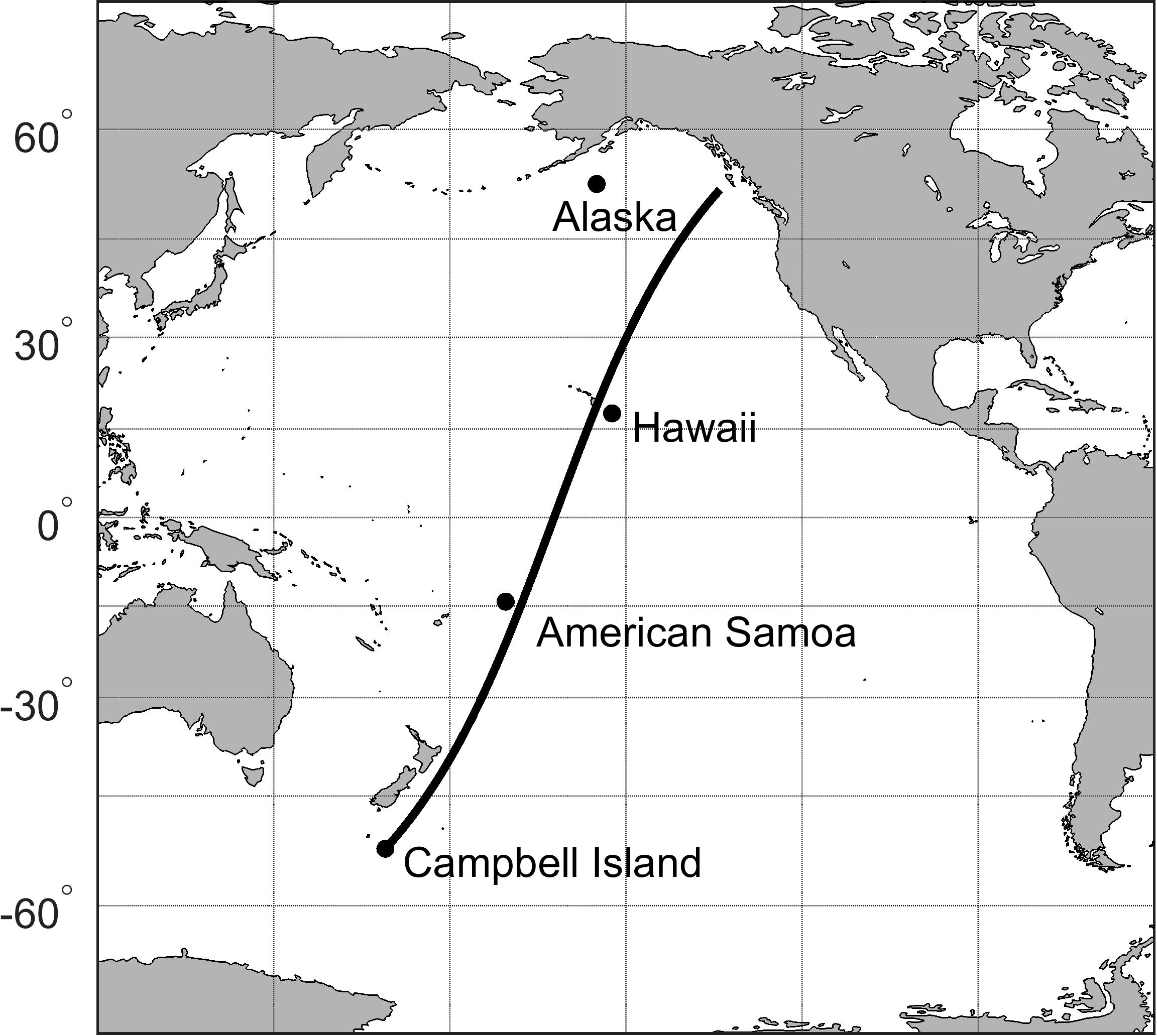
Figure 1 Selected buoys in the Pacific Ocean (Campbell Island, American Samoa, Hawaii, Alaska). The solid line shows a Great Circle path from Campbell Island.
The buoys were located at Campbell Island (Southern Ocean), American Samoa, Hawaii and Alaska. As shown in Figure 1, these buoys are approximately located on a Great Circle path from Campbell Island. This is approximately the same path considered by Snodgrass et al. (1966).
Table 1 shows the details of each of the buoys including: location, buoy type, sampling frequency, water depth and period for which data were extracted. Note that there are a range of buoys near Hawaii which could have been selected for this site. Examination of data from these buoys indicated that buoys to the north of the islands (51000, 51001) were clearly influenced by shadowing. As such, Buoy 51004, which is Southeast of the islands and open to Southern Ocean swell was selected for this location.

Table 1 Details of the buoys used in the study.
The combined instruments (Sentinel-1 SAR, CFOSAT and buoys) provide a unique dataset to study swell propagation across the Pacific. The buoy located at Campbell Island provides a direct measure of the directional spectrum at, or close to, the generation site of the swell. Such Southern Ocean data are extremely rare (Smith et al., 2021; Young et al., 2020; McComb et al., 2021). The subsequent buoys on the Great Circle to Alaska provide a useful insight into the swell propagation, but as identified by Snodgrass et al. (1966) and as shown below in Figure 2 of Section 3, the dominant swell propagation path is further to the southeast (from Campbell Island to Central America). Except for the data from the Campbell Island buoy, the data from the rest of the buoys were not used beyond the validation process due to a relatively smaller number of swell events along this path. To monitor these more energetic swell pathways, and greatly increase the quantity of data, the satellite data have been utilized.
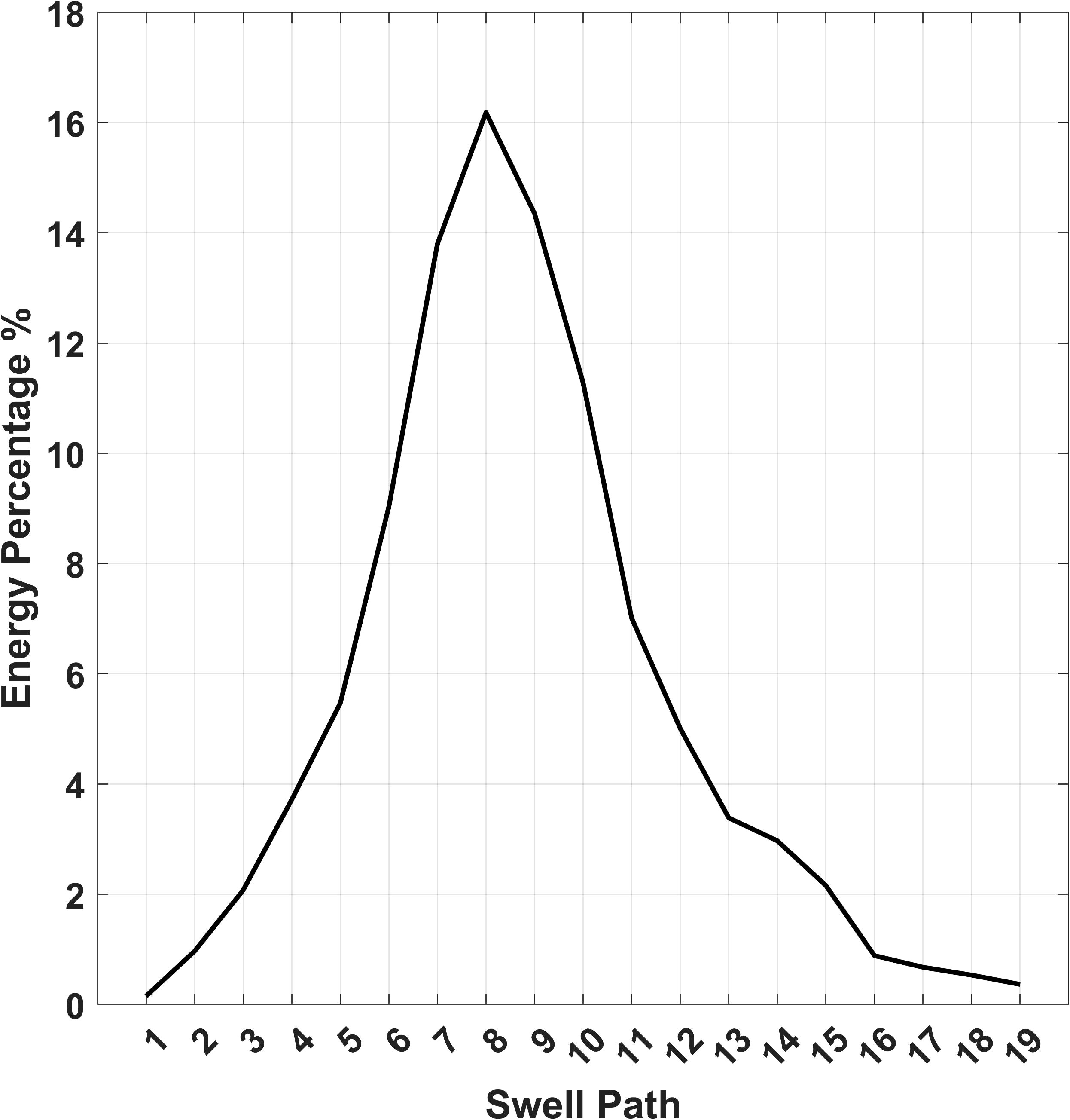
Figure 2 Distribution of swell energy propagating along each of the swell paths from Campbell Island for the years 2017-2020 calculated from WW3 modelled directional spectra.
The Campbell Island buoy data can be obtained as in McComb et al. (2021) and data from the other buoys from https://www.ndbc.noaa.gov/.
3 Swell event identification and tracking
3.1 Swell event identification
As detailed in Section 2, a global implementation of the WW3 wave model was run with ERA5 defined wind and sea ice for a period of 4 years from 2017 – 2020 (Cabral et al., 2022). Initially, ST6 source term physics was used. Figure 3 shows a comparison of WW3 and Campbell Island buoy values of significant wave height, , peak wave period, and peak wave direction, for the month of August, 2018. As seen in the figure, the model reproduces these bulk parameters in the swell generation region well over this period, adding confidence that the model is a useful diagnostic tool to represent the subsequent swell propagation.
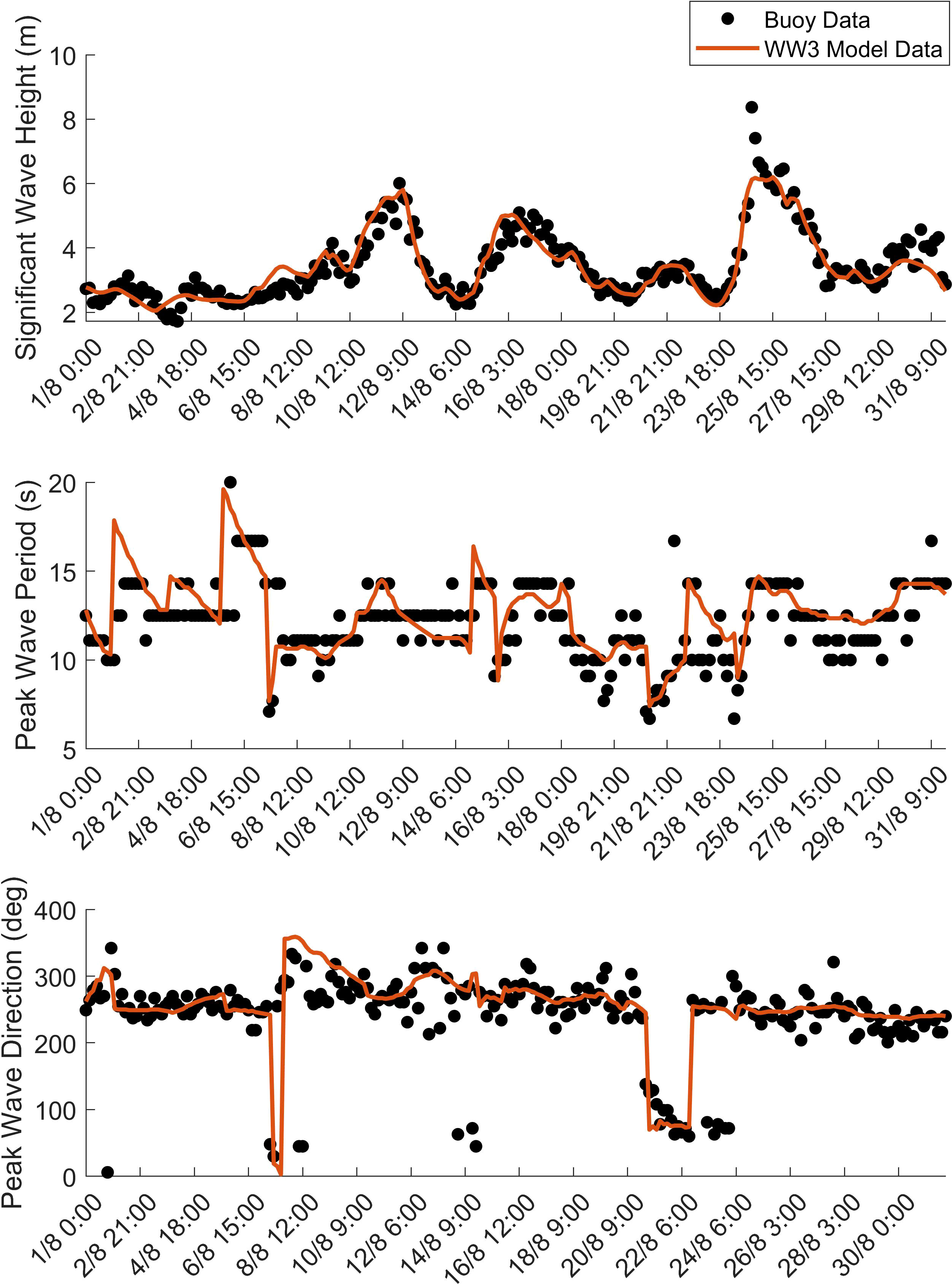
Figure 3 Comparison of values of significant wave height, , peak wave period, and peak wave direction, between buoy and WW3 model (ST6) at Campbell Island. Data are shown for the month of August 2018.
Previous studies of swell propagation and decay have generally observed swell at specific locations and then back propagated along Great Circle paths to the approximate generation site (Ardhuin et al., 2009; Collard et al., 2009; Jiang et al., 2016b). In the present case, both buoy and validated WW3 model results are available in the approximate generation region. Therefore, we rely on these data to identify swell generation events. Swell events generated in the region of Campbell Island were selected by identifying storm peaks with equal to or greater than 4m. Both model and buoy data were used for this purpose, producing similar results, as seen in Figure 3. Once these high-energy events were identified, a further filtering was undertaken by selecting events with waves travelling toward angles between 0°to 180° (nautical convention where angles are measured clockwise from North and waves are propagating to this direction) to capture only the events where swell will propagate across the Pacific Ocean.
For this study, 19 swell paths (Great Circles) equally spaced at 5° angles were defined covering the Pacific Ocean as shown in Figure 4. The angle between the peak wave direction of waves at Campbell Island and the azimuth of each swell path was calculated and if this angle falls within a wedge of ±5° from a defined swell path, that path was adopted as the propagation path for the specific event.
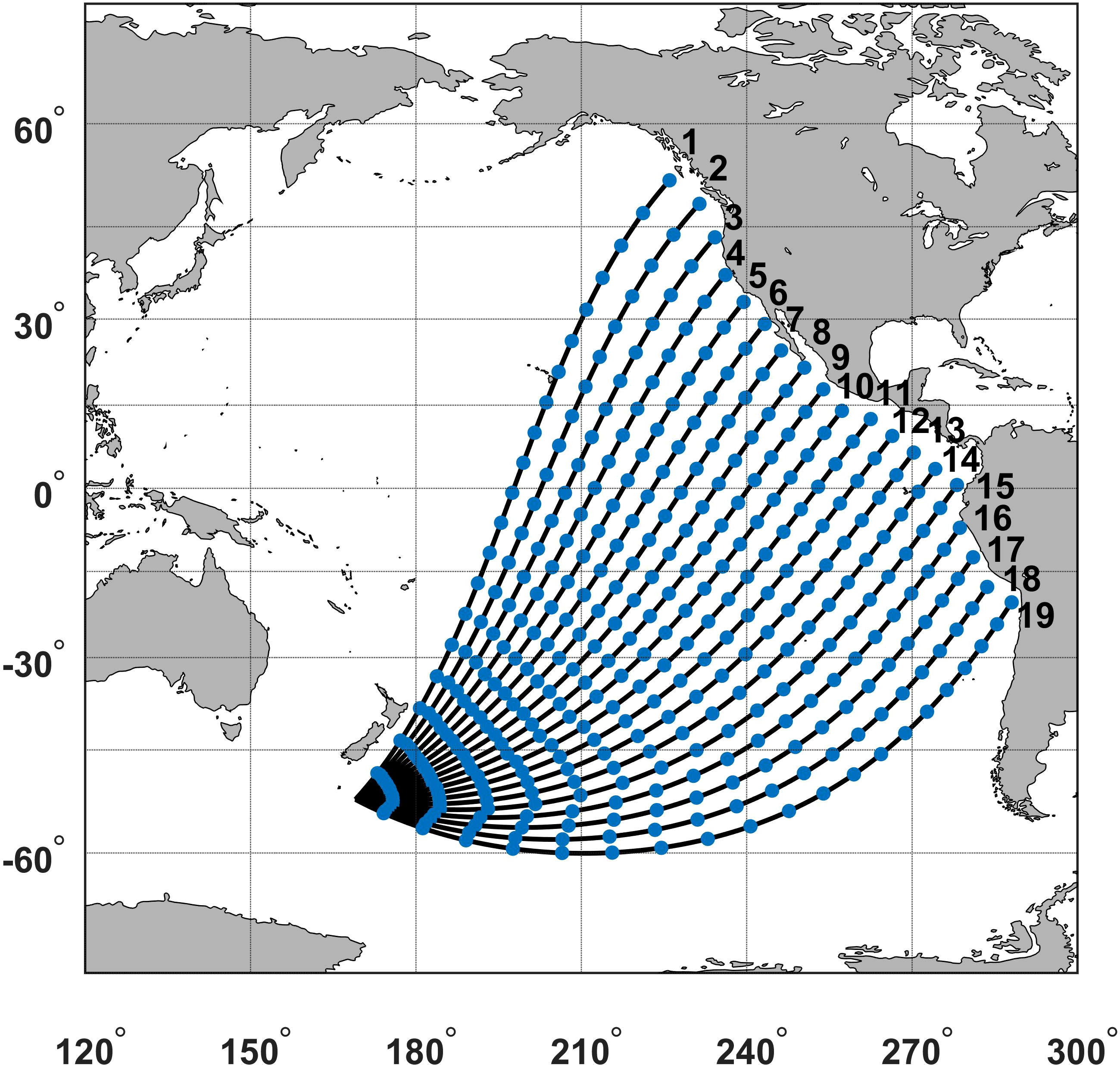
Figure 4 Potential Great Circle swell paths at 5° intervals across the Pacific Ocean from Campbell Island.
Using the above selection method, a total of 708 storms were identified, with Table 2 showing the distribution of storms for each year. Not surprisingly, the majority of the storms were found in the Southern Hemisphere winter months of July – September.
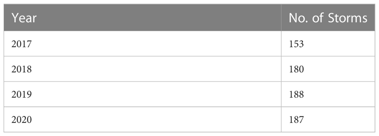
Table 2 Number of storm peaks identified at Campbell Island for which swell propagated along the Great Circle paths in Figure 4.
3.2 Swell energy propagation from the Campbell Island region
With the assumption that swell energy propagates at its group velocity, the group velocity, , for the waves at the peak of each identified storm event at Campbell Island was computed using linear theory, as in Equation (1)
With the computed value of , the energy from each swell generation event was tracked along its respective swell path. Since satellite data are available only at discrete times along satellite ground tracks, it is necessary to identify times when there is a satellite overpass at the approximate arrival time of the swell. At 500 km intervals along the swell path, a region of 1.5-degree radius was identified. These locations are shown by the blue dots in Figure 4. If the computed swell arrival time at the location and a satellite ground track through the search circle agreed within a period of day, this was considered as an approximate “match up” between the arriving swell energy and satellite data. This swell tracking process was undertaken for Sentinel-1A and 1B for the years 2017 – 2020 and for CFOSAT for the period from Aug 2019 – Dec 2020.
A swell partition was then applied to both satellite and WW3 model spectra which satisfy the above “match-up” criteria. The partition was applied by considering only components with a frequency less than 0.08Hz and a directional wedge ±15° of the local azimuth of the Great Circle propagation path. The total energy of this frequency-direction partition was then calculated for both satellite and WW3 model spectra. As there will be multiple satellite spectra which satisfy the “match up” criteria for each satellite pass (i.e., 1.5-degree search radius and day search window), the maximum energy values were selected for the satellite observations. This is consistent with the aim to identify the arriving swell from the energy peak observed at the approximate generation region (Campbell Island). The spectral peak frequency was also calculated from the partitioned spectra. The spatial and temporal window adopted (1.5° and day) is significantly larger than typically used for buoy/satellite collocations for altimeter calibration studies (Ribal and Young, 2019). However, the context is quite different, as we are here searching for the arrival of a swell peak at the location. Thus, in addition to the window size, the data selection is constrained by the search for a swell peak.
As an example, Figure 5 shows time series plots at points along the Great Circle path number 8 in Figure 4, tracking the values of peak wave period for the propagation of a swell event directed along this path. The peak of this storm event was identified at Campbell Island at 05.00 UTC on Aug 3rd, 2019, with a value of 14s. The vertical blue lines show the predicted time of arrival based on the calculated value of the group velocity (Equation (1)). The solid lines show the WW3 model values of from the swell partition, as defined above. Therefore, if the swell arrives at each location at the predicted time, the local values of should also be 14s. Values of from both Sentinel-1 SAR and CFOSAT are shown as data points in each of the panels. Note, that for CFOSAT, there are a range of potential imaged regions that satisfy the above co-location criteria, represented by the multiple data points at the same co-location time.
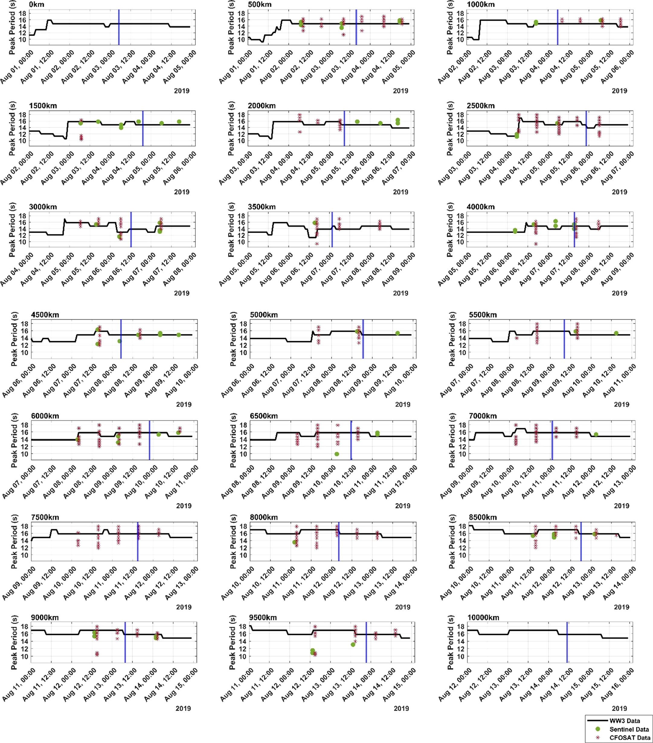
Figure 5 Values of peak wave period as a function of time from Sentinel 1-SAR, CFOSAT and WW3 (black solid line) at selected values along Great Circle path 8 for a storm event on Aug 3rd at 05.00 UTC at Campbell Island. The distance from Campbell Island along the Great Circle path is shown by the number in the upper left of each panel.
Due to frequency dispersion, the panels typically show a rapid increase in as the first “fore runners” of swell arrive. The values of then gradually decrease as higher frequency (smaller ) components arrive. Although there is some variability in the recorded values of satellite data, there is general agreement between the satellite data and the WW3 model, in terms of values of . At longer values of propagation distance (greater than 6,000km), the values of from both the model and satellite data, at the times of the expected arrival (blue vertical lines) are larger than the linear propagation model (i.e. >14s). This suggests that processes other than just propagation at the group velocity are active in the swell transformation across the Pacific.
The distribution of swell energy from all identified swell events across the swell paths was calculated using the WW3 modelled directional spectra and shown in Figure 2. To form the figure, the energy within the swell partition for each identified swell generation event, was integrated over all frequencies and directions. This total energy was then associated with the swell path closest to its peak wave direction. Figure 2 shows the distribution of the energy totals formed by summing over all swell events. It is clear that the principal direction of swell energy propagation is along paths 7, 8 and 9. These paths run from Campbell Island approximately to the northeast towards Central America.
4 Swell decay rate calculation from observations
As noted above, there are two broad processes believed responsible for the observed reduction, at a measurement location, of energy for propagating swell. These are the spatial spreading of wave energy due to frequency dispersion and angular spreading and decay due to physical processes (Jiang et al., 2016b).
Collard et al. (2009) and Ardhuin et al. (2010) showed that with the assumption of a point generation source for the swell, and at a location distant from this generation source, the frequency dispersion and spherical spreading can be described by
In Equation (2), is the swell energy and is the angular distance from the generation source (i.e. ), where is the propagation distance on the Earth’s surface of the swell over a period of time equal to at group velocity on the Earth of radius . The term accounts for the frequency dispersion and the term for the spherical spreading.
The spatial dissipation rate of swell along a great circle path was represented by Ardhuin et al. (2009) using Equation (3), where dissipation rate is assumed constant.
Ardhuin et al. (2010) showed that the spatial dissipation rate, can be represented by
where is the swell energy at location measured along a Great Circle path and is the swell energy at a reference location, taken far from the assumed point generation source. This value has typically been taken as 4000km (Ardhuin et al., 2010; Jiang et al., 2016b). Equation (4) can be linearized as
Values of and can be determined from a least squares fit of Equation (5) to observed values of along a Great Circle path.
Using the swell selection process described above, at each of the regularly spaced points (500km intervals) along the Great Circle paths, values of were calculated from the Sentinel-1 SAR and CFOSAT directional spectra partitioned in the frequency band of 0 – 0.08 Hz and ±15° in the directional band. The space (1.5-degree radius circle) and time ( day) search intervals, define the location and time of the arrival of the swell event generated at Campbell Island. The satellite datasets were searched for observations within these space/time windows. Multiple satellite observations typically occur within the search window at each location along the swell path. Consistent with the fact that the maximum wave energy of the storm event was selected at Campbell Island for the swell initiation, the maximum energy case from this range of values was also taken as the observed satellite swell energy at each location along the Great Circle path. Data at each of the locations (500km intervals) along the Great Circle path for each swell event were then used in a least squares curve fit to Equation (5), and a value of the swell decay coefficient determined for each storm event. Data within 4000km of Campbell Island were excluded, as they are considered to be in the nearfield (see above). Figure 6 shows the values of the swell decay coefficient as a function of the significant wave slope at 4,000km for Sentinel-1 SAR and CFOSAT datasets. The significant wave slope is defined as the significant wave height of the swell, divided by the swell wavelength, . The data shown is for all observed swell cases at Campbell Island, over a range of swell wavelengths, .
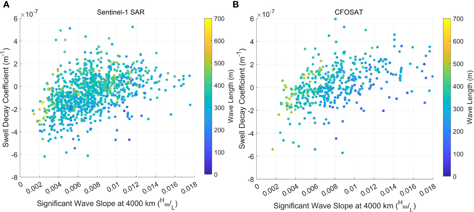
Figure 6 Swell decay coefficient, as a function of significant wave slope at 4,000km for (A) Sentinel-1 SAR data and (B) CFOSAT data.
The analysis in Figure 6 was undertaken to demonstrate that the present data is comparable to previous studies, rather than to define values of the swell decay coefficient, . The detailed analysis of the swell evolution is considered in the following sections, using the wave model as a diagnostic tool. The present results give consistent values of for both Sentinel-1 SAR and CFOSAT, ranging between m-1. Positive values of represent decay. Such values are of similar magnitude to previous studies (Ardhuin et al., 2009; Collard et al., 2009; Jiang et al., 2016b; Stopa et al., 2016c). The data generally shows values of increase with increasing significant wave slope. There is, however, significant scatter in the data, with also negative values of (amplification). Previous studies have considered error analyses, showing a range of potential error sources, including: a 20% deviation in (approximately m-1 for ) due to the storm shape (Collard et al., 2009), errors in the curve fitting approach of around m-1 (Jiang et al., 2016b) and errors due to the point source assumption of magnitude m-1 (Ardhuin et al., 2009).
The present analysis does not apply a filtering criterion that the wind speed along the propagation path must be relatively low (Young et al., 2013), although the data is partitioned to frequencies less than 0.08Hz, meaning that there will be little wind input for all but the strongest wind speeds. Two other error sources, which will be subsequently considered, are current refraction and island sheltering. The distribution of the values obtained for the Sentinel-1 SAR and CFOSAT data are shown in Figure 7. As seen in this figure, the mean of both datasets is approximately zero, (i.e., swell both decaying and amplifying) showing the significant errors in this type of analysis.
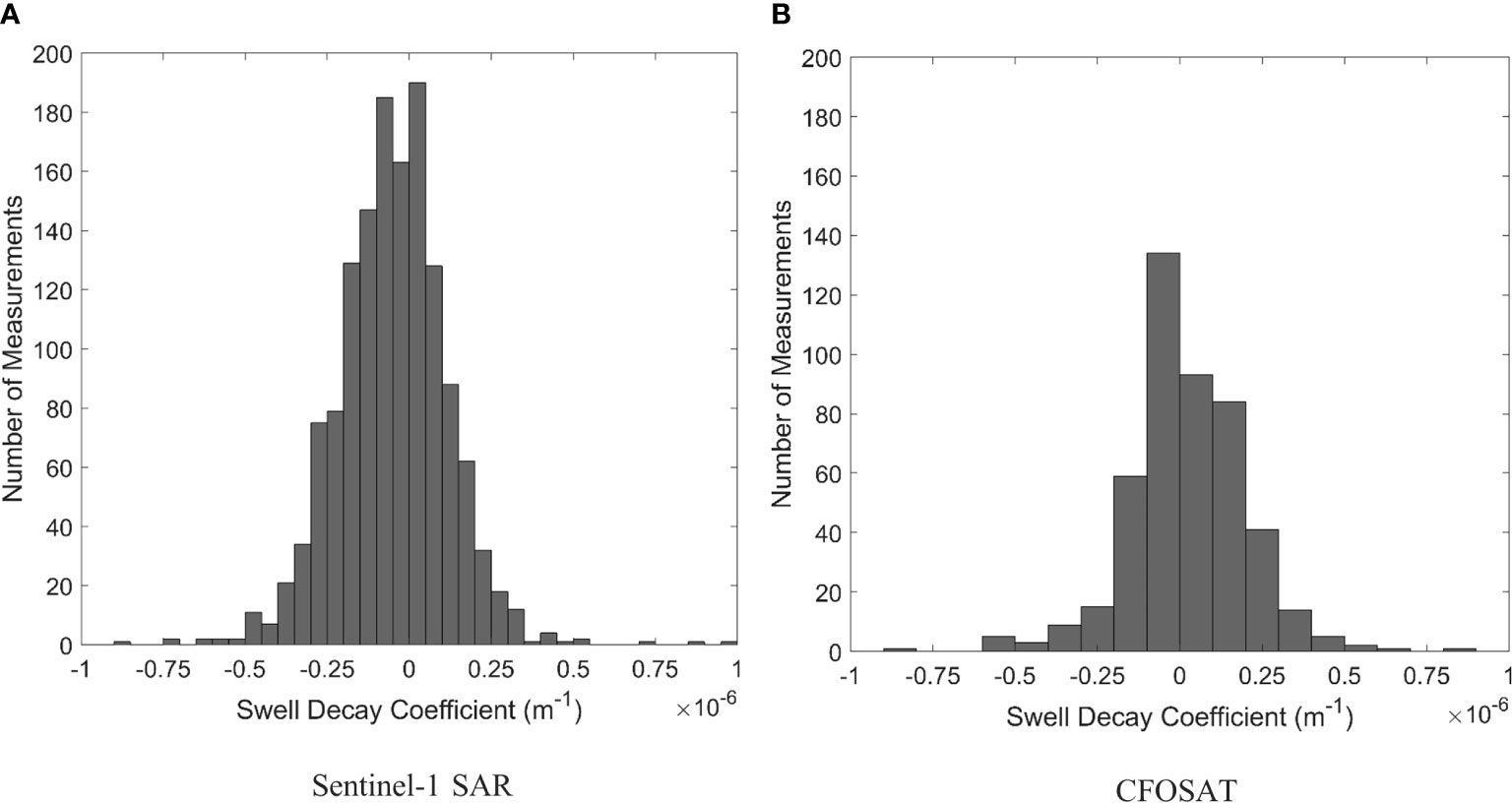
Figure 7 Statistical distribution of the swell decay coefficient, from (A) Sentinel-1 SAR data and (B) CFOSAT data.
5 Swell modelling with WAVEWATCH III and standard ST4 and ST6 source term packages
The calculation of an empirical decay coefficient, such as the analysis above provides little insight into the physical process responsible for the observed swell decay. The analysis also relies on the assumption that the swell is generated from a point source. Analyzing the data using a spectral wave model, such as WW3, potentially overcomes these limitations. Such a model can provide high sampling resolution in space and time and will account for both frequency and angular dispersion as well as wave current effects (Liu et al., 2021). In addition, the model can include impacts such as interaction with local winds, current refraction, and nonlinear wave-wave interactions, together with explicit source terms for swell decay.
The WW3 model represents the evolution of the wave action equation (Equation (6)) in space and time (Komen et al., 1984; Tolman, 1990)
where is the wave action and is the radian frequency. The wave related physical processes impacting the wave action spectrum, are included as a summation of multiple spectral functions in the total source term ( . Spectral source functions typically included for deep water conditions are: - atmospheric input from following wind, - decay from opposing winds, - non-linear wave-wave interactions, , white-cap dissipation and , swell decay (Komen et al., 1994; Young, 1999). Note that in many publications it is not uncommon to call the sum the wind input and the sum the dissipation. As we are interested in each of these components in the present application, we explicitly define each term. The propagation of the spectrum on the Earth’s surface (terms on left hand side of Equation (6)) accounts for frequency dispersion, lateral spreading and current refraction (if included), here modelled using a third-order propagation scheme to reduce numerical dispersion (Wingeart et al., 2002).
There are a range of source term packages available within the WW3 model. In the present application, we have investigated both the ST4 (Ardhuin et al., 2010) and the ST6 (Liu et al., 2021) packages. These packages are described briefly in the following sections. In each package, the nonlinear term, is solved using the Discrete Interaction Approximation (DIA) (Hasselmann et al., 1985).
5.1 ST4 parametrization
The atmospheric input term in the ST4 source term package is based on the earlier ST3 version, which parameterizes the air pressure – wave slope correlation (Miles, 1957; Janssen, 1982) as proposed by Janssen (1991) and Abdalla and Bidlot (2002).
where is a dimensionless constant growth parameter, is a constant describing the spreading of the atmospheric input, the terms define the magnitude of the surface stress, is the von Karman constant (0.41), and are the densities of air and water, respectively, is the wind friction velocity, is the wind direction, is the wave action spectrum which is a function of wavenumber and direction and is a wave age tuning parameter.
The ST3 package also included a term to potentially account for linear dissipation of swell (Janssen, 2004).
where is a roughness length, m. The value is set to 1 if damping is to be included and 0 otherwise and is the wave phase speed. The physical basis of Equation (8) is not clear and it seems to be intended to be a combination of swell dissipation and negative wind input.
The ST4 package (Ardhuin et al., 2010; Rascle and Ardhuin, 2013; Stopa et al., 2016b; Stopa, 2018) applies a reduction to in Equation (7) to balance changes made to the dissipation term, used. In this package, the input is limited only to spectral components with a positive input (i.e., not opposing wind decay).
In contrast to Equation 8, the swell dissipation term in the ST4 package is formulated as the summation of a linear viscous, , and a turbulent, term (Ardhuin et al., 2009)
where and are empirical weighting terms. As summarized by Young et al. (2013) flow within the air above waves is almost always turbulent and hence the turbulent term in Equation (9) dominates. The turbulent term is given by (Ardhuin et al., 2009) as
where is the significant orbital velocity and Ardhuin et al. (2009) report the decay coefficient based on SAR observations of swell decay. In comparisons of model results with observations, it was found that the model tended to underestimate large swells and overestimate small swells (WW3DG, T.W.I.D.G 2019). To correct this, the decay coefficient was represented as a function of wind speed and direction.
where is the friction factor given by the theory of Grant and Madsen (1979) and , and are tuning parameters.
Although parameterizations such as Equation (11) may enhance model performance, they, coupled with the tuning parameters in Equation (9) effectively mean that the swell decay term, is largely reduced to a tuning parameter to optimize model performance. In addition, the inclusion of a dependence on wind speed in Equation 11 means that this “swell dissipation” term can also include some impact of negative wind input for opposing winds.
5.2 ST6 parametrization
The atmospheric input term in the ST6 package is based on field measurements of wave-induced pressure over waves conducted at Lake George, Australia (Donelan et al., 2005; Young et al., 2005; Donelan et al., 2006). These experiments highlighted a number of processes, contributing to , not previously considered, including: (i) air flow separation over steep waves, (ii) dependence of wave steepness and (iii) enhanced atmospheric input in the presence of wave breaking. The ST6 atmospheric input term takes the form:
where
In the above, is the spectral saturation, which is a measure of wave steepness; is the inverse of the spectral narrowness (Babanin and Soloviev, 1987) and is a scaling wind speed. Following Komen et al. (1994) and Rogers et al. (2012); Liu et al. (2019) adopted . The wind growth coefficient α is equal to 1 for following winds or set to for opposing winds.
Wave decay in opposing winds (negative wind input, ) is not well understood, either theoretically or experimentally. There have been no field measurements of the active processes and only limited laboratory studies (Young and Sobey, 1985; Donelan, 1999). The ST6 package adopts the formulation proposed by Donelan (1999), that is, the same representation as for following wind (Equation (12)), but with a value for in Equation (13) (Liu et al., 2019). That is, is approximately 10% of for the same wind. The laboratory data supports the conclusion that and the value of 0.05 was proposed by Liu et al. (2019) by model tuning against measured buoy data.
Swell dissipation in the ST6 package follows the approach of Babanin (2011) and Young et al. (2013) and takes the form
where the term is wave steepness dependent
By tuning model performance against buoy and altimeter observations, Liu et al. (2019) obtained .
As noted above, the ST6 package includes an explicit negative wind input term, through opposing winds in Equation 12. For the case of swell propagation through regions of near zero winds, the form of Equation 16, means there will be decay due the negative relative wind speed. In contrast, the form of Equation 11, means there will be approximately no comparable negative wind input for ST4 in such a case. Therefore, one might assume that negative wind input would be larger in ST6 than ST4 for swell propagation.
5.3 Initial WW3 model runs
Initially, the WW3 model was run for both the standard ST4 and ST6 source term packages, as specified below, for a period of 4 years from 2017 to 2020.
The ST6 package has few “tunable” parameters. One such parameter is the CDFAC term, which scales the wind input. This was chosen as CDFAC=1.0, which was the original calibration factor of ST6 with CFSR winds. Both and were set at their default values: and . Two simulations were performed: one with the model forced with ERA5 winds and ERA5 sea ice, and the second with the same ERA5 wind and sea ice but with the inclusion of COPERNICUS-GLOBCURRENT currents (https://resources.marine.copernicus.eu/product-detail/MULTIOBS_GLO_PHY_REP_015_004/INFORMATION). A regular, 1 degree resolution grid, covering the region 79.50 N to 79.50 S was used. A model “spin up” of one month was used and data were output hourly.
A model run with the ST4 package (TEST471) was also undertaken with currents added for the same model setup. The following parameters were set in TEST471: , , , -0.018 and 0.022 (WW3DG, T.W.I.D.G 2019).
Figure 8 shows the time series of significant wave height, , at Campbell Island for the wave buoy and the two ST6 model simulations (with and without currents) for October 2018.
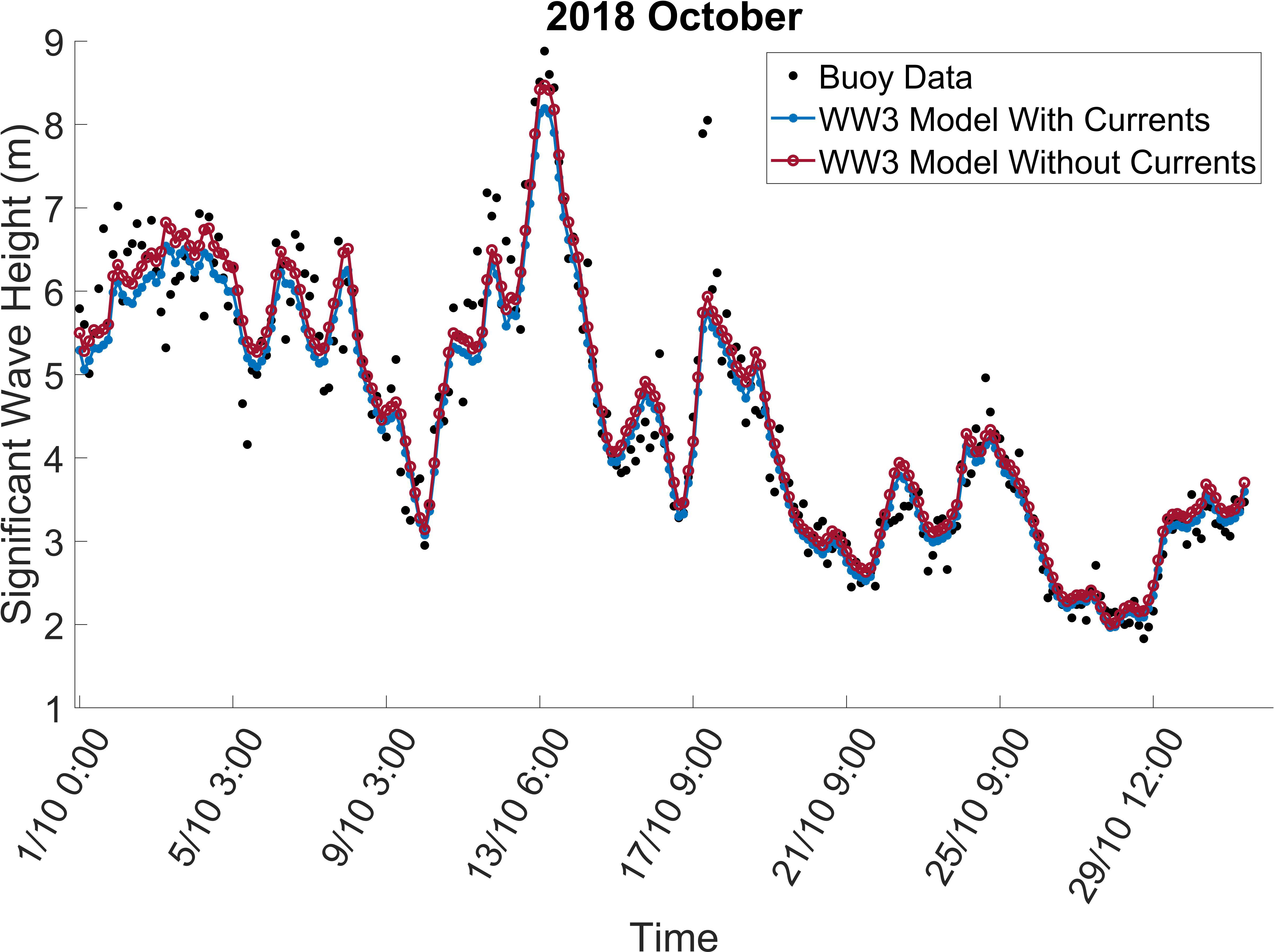
Figure 8 Significant wave height at Campbell Island for October 2018. The figure shows buoy data, together with WW3 ST6 results with and without the inclusion of currents.
The model results are in good agreement with the buoy data and the addition of currents make only a very small difference in model performance compared to the buoy. Absolute values of bias with and without currents are less than 4%. Although currents may not have a significant impact at Campbell Island, subsequent swell propagation from this location may be more impacted by current refraction. Subsequent tests (see Figure 9), however, showed that current effects also do not have a significant impact on the swell propagation.
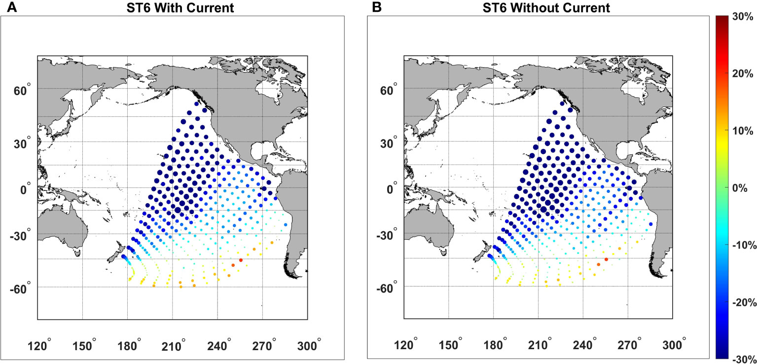
Figure 9 Relative normalized bias () for the original ST6 source term package for Sentinel-1 SAR (A) with currents and (B) without currents. The size and color of the markers are proportional to the values of the relative normalized bias.
Figure 10 shows the time series of significant wave height at Campbell Island for October 2018 for the buoy and the ST4 and ST6 runs, both with the inclusion of currents.
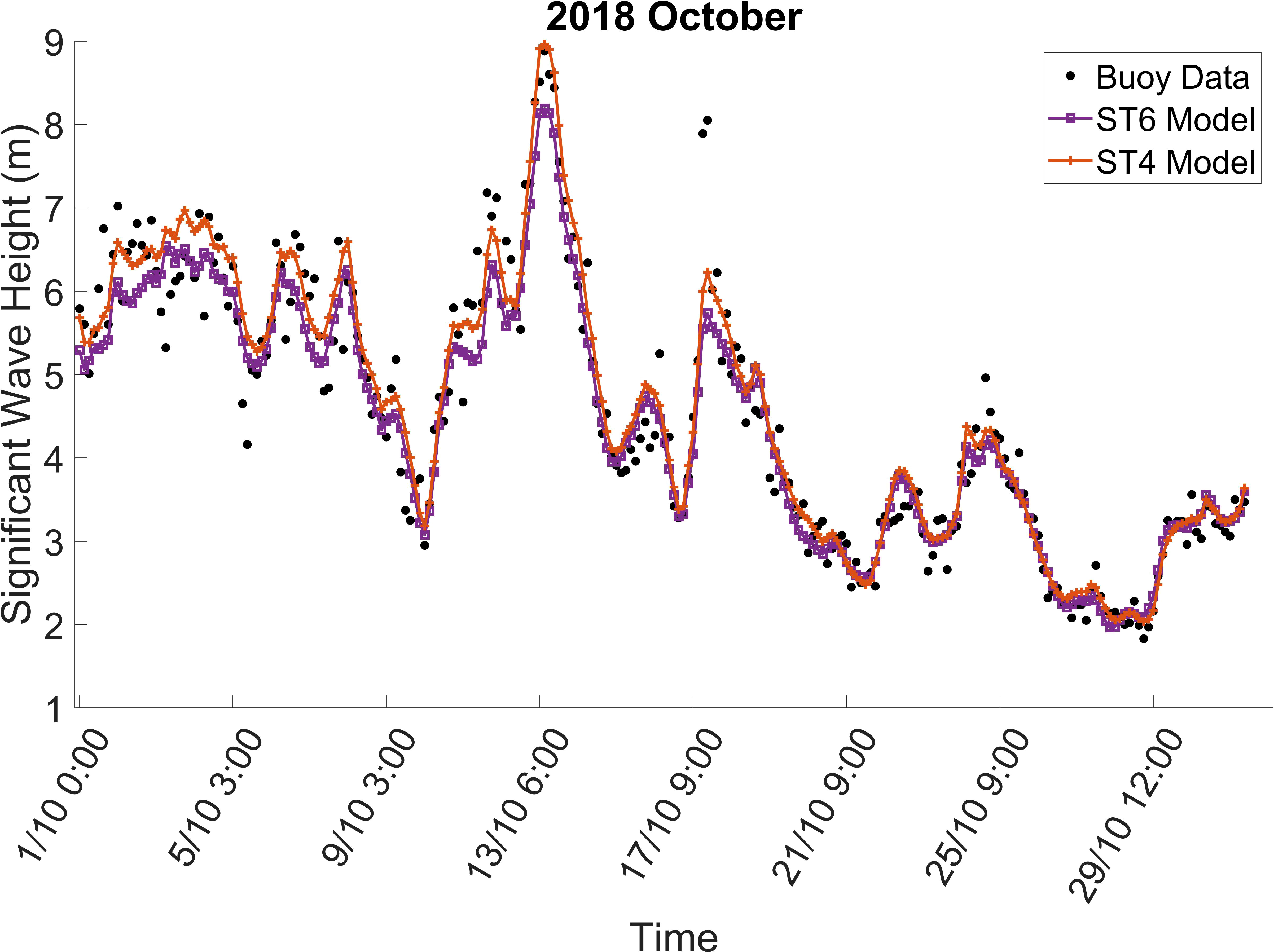
Figure 10 Significant wave height at Campbell Island for October 2018. The figure shows buoy data, together with WW3 results from ST6 and ST4 source term packages.
The results in Figure 10, indicate that both source term packages reproduce the significant wave height at Campbell Island well. However, the ST4 package shows greater skill in reproducing the wave height peaks, suggesting that either: it models the physics more adequately, it is better calibrated or the process it uses to determine the wind forcing, performs better. Such a comparison cannot determine which of these processes is most important. The key finding for the present context, however, is that both source term packages adequately model wave conditions in the swell generation region of interest for the present application.
5.4 Validation of WAVEWATCH III model against observational data
The results in Figures 8, 10 show the performance of the model in reproducing significant wave height in the swell generation region around Campbell Island. However, these results do not validate model performance in terms of swell propagation across the Pacific.
As described in Section 3, for each of the swell generation events identified at Campbell Island, the times of arrival at the specified locations along the Great Circle paths (see Figure 4) were determined within an arrival window of 1 day. Sentinel-1 SAR and CFOSAT passes through a 1.5 deg radius region around each of these locations were defined and the satellite passes through these regions extracted. Model data were compared to satellite data that met these time/space windows to validate model performance across the Pacific.
Due to its imaging mechanism, SAR cannot resolve wavelengths shorter than 150m. Therefore, integration of the SAR spectrum will underestimate the true significant wave height (i.e., energy at higher frequencies is not considered) (Khan et al., 2021). Therefore, we term the wave height obtained from integration of the SAR spectrum as the “SAR wave height”. To obtain comparable results from the WW3 model for validation purposes, the WW3 spectra were integrated over the bandwidth from 0 Hz to the high-frequency SAR cutoff-wavelength. In the case of CFOSAT, data of the 10-degree incidence angle beam were selected as it has been shown to produce the most reliable results (Hauser et al., 2021; Le Merle et al., 2021). For the comparison with CFOSAT, the full directional spectra of both CFOSAT and WW3 were used as there is no, high-frequency imaging issue in the CFOSAT instrument. The frequency range of CFOSAT was 0.06Hz – 0.26Hz, while for the WW3 model the range was 0.03Hz - 0.95Hz.
Figure 11 shows reasonable agreement between the WW3 ST6 model and both Sentinel-1 SAR and CFOSAT, with normalized biases of -15.1% and -13.8%, respectively (i.e., model is less than satellite data). At Campbell Island (Figure 8), the ST6 model showed a normalized bias (over the same period) of -2%.

Figure 11 Validation of WW3 ST6 wave height against Sentinel-1 SAR and CFOSAT 10° beam for all the swell paths across the Pacific (Figure 4). (A) SAR wave height versus WW3 wave height determined over the same frequency range (B) CFOSAT significant wave height versus WW3 significant wave height.
The comparison between the Sentinel-1 SAR and CFOSAT satellite data and the ST4 model is shown in Figure 12 for the same data period as Figure 11. Again, there is a negative bias, of magnitude -10.1% for Sentinel-1 SAR and -9.03% for CFOSAT. Hence, the two source term packages perform similarly, and both appear to underestimate significant wave heights across the Pacific during swell events. Note that as these validation results consider the full available frequency ranges of both satellite instruments, the observed differences cannot be attributed to swell propagation alone. Local wind forcing may also play a role in the observed negative bias.
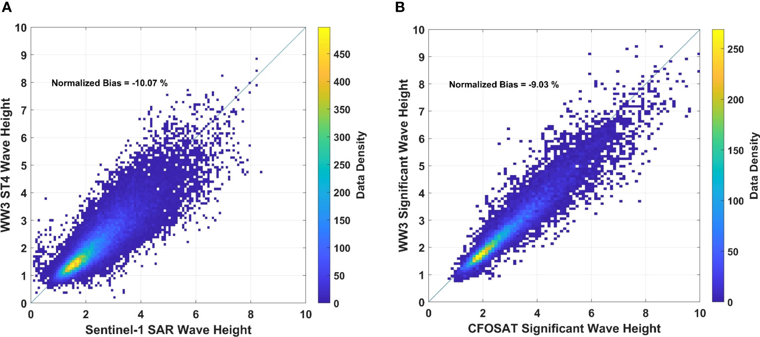
Figure 12 Validation of WW3 ST4 wave height against Sentinel-1 SAR and CFOSAT for all the swell paths across the Pacific (Figure 4). (A) SAR wave height versus WW3 wave height determined over the same frequency range (B) CFOSAT significant wave height versus WW3 significant wave height.
5.5 Swell modelling performance
The WAVEWATCH III model performance, in terms of swell propagation, was analyzed by calculating the normalized bias of the model relative to the observed wave heights from the respective satellites along each propagation path (Equation (19)). Initially, data were filtered such that only spectral components less than 0.08Hz (swell components) and within of the azimuth of the Great Circle path (components propagating along this swell path) were considered. However, the directional filtering resulted in very large values of bias, due to the different directional spreading between model and satellite data. It is well known that the discrete interaction approximation to the nonlinear source term in the WW3 model results in excessively broad directional spreading (Zieger et al., 2015). As a result, the directional filtering was not subsequently used. Rather, we take the mean direction of the model at Campbell Island and assume the energy propagates along the Great Circle path closest to this direction (i.e., 5°). The full energy of the waves at Campbell Island is assumed to propagate along the path with no directional filtering. Similarly, the full directional spread of both model and satellite data is considered at each matchup location/time. This means that it is possible for some energy to arrive at locations being considered which did not originate at Campbell Island and propagate along the Great Circle path under consideration. Also, as Sentinel-1 SAR data does not capture higher frequency components, the cutoff wavelength value from Sentinel-1 SAR was again applied to WW3 directional spectra for the comparisons. However, as the data are filtered to retain only components for Hz, this second frequency filtering has insignificant impact. We term this filtered energy, swell energy, and its resulting wave height the swell significant wave height, . The normalized bias of these swell components thus becomes
where N is the number of observations.
The normalized bias was calculated at each of the locations along the 19 Great Circle paths (separated by 500km) from Campbell Island. In order to understand the trend in the bias along each propagation path, the values of normalized bias, at point 1 (500km from Campbell Island, see Figure 4) were subtracted from the remainder of the points along that Great Circle path. The results for the original ST6 source term package are shown in Figure 9 for the 19 swell paths for Sentinel-1 SAR for cases both with and without currents. For visual interpretation, both the size and the color of the markers in Figure 9 are varied according to the magnitude of the relative bias, .
The vast majority of the points across the Pacific Ocean have a negative bias, which increases in magnitude with distance along the swell propagation path. This suggests that the model dissipates more energy than indicated by the satellite (SAR) data. The study by Stopa et al. (2016a) also saw a stronger dissipation of swells far away from storms. The negative bias along swell paths 5 to 7 (see Figure 4) increase significantly in magnitude and then decrease in the central Pacific. The region in the central South Pacific where there is this apparent discontinuity in the normalized bias, corresponds with the location of South Pacific islands. Also, the impact of the Galapagos Islands is seen for the final few points of swell path 14. These final points close to the coastal regions of North and South America also show an increase in the magnitude of the relative normalized bias. These results generally indicate that the swell decay in the WW3 model with the ST6 source term package is larger than indicated by the satellite data. In order to model such small islands, we adopted the default sub-grid scale blocking approach of Chawla and Tolman (2008) in WW3. An alternative explicit source term for such unresolved obstacles has been proposed by Mentaschi et al. (2018). Further investigation of island impacts was beyond the scope of the present work and not considered further.
In addition, in the presence of islands, the model also dissipates more energy than indicated by the satellite data. An examination of Figures 9A, B indicates that currents have little impact on the magnitude of the swell decay across the Pacific.
It is noticeable that for the swell paths to the south (paths 17, 18, 19), the values of relative swell bias are much closer to zero, indicating the model and observations are in better agreement. These regions remain in the strong wind belts of the Southern Ocean/Southern Pacific, where it is likely that the frequency bands under consideration (0 to 0.08Hz) are still receiving energy from the local (strong) winds. Therefore, these swell paths are more likely responding to the impacts of all source terms, not simply swell decay. As we know the model performs well at Campbell Island, it is not surprising that these paths also agree well with the satellite data (Bi et al., 2015).
6 Optimization of WAVEWATCH III ST6 source term package
6.1 WAVEWATCH III test runs
The above results show that the ST4 and ST6 source term packages have similar performance. As seen in the formulations in Equations (7) to (18), ST6 has a clearer separation of the physical processes of swell decay and negative wind input. In contrast, ST4 includes terms which can be considered negative wind input as part of the swell decay. Due to the clearer descriptions of these separate processes in ST6, we select this package for further analysis.
The results in Figure 9 indicate that there are significant differences in terms of normalized bias between the ST6 WW3 model and observed swell propagation across the Pacific. In order to understand the reasons for these differences and to potentially improve model performance, a series of three tests were undertaken. Each test was designed to investigate elements of the model physics and to understand sensitivity to individual processes in the predicted swell propagation. It should be noted that, the intention here is to explore the physical processes active and not to “tune” the model. It is likely that optimization of the swell decay using the approach/data available here, without subsequent global tuning, would actually result in poorer overall global model performance. As shown by Liu et al. (2019), model tuning requires careful consideration of the interaction of different source terms.
6.1.1 Test 1: Scaling coefficient in the swell dissipation term
As the results in Figure 9 appear to indicate there is excessive swell dissipation in the WW3 ST6 model, the first test involved a reduction (halving) of the value of the scaling coefficient in Equation (18). The original value of in the ST6 configuration was 0.0041 (Liu et al., 2019) and for this initial trial, the value was reduced to 0.00205. Such a reduction can be expected to reduce the overall swell dissipation and hence reduce the magnitude of the values of normalized bias.
6.1.2 Test 2: Exponent of the wave steepness term in the swell dissipation formulation
Zieger et al. (2015) and Liu et al. (2019) assumed that the term in (Equation (17)) is a function of wave steepness. This is a reasonable assumption but there is little theory to support the assumption. In the absence of further information, it was assumed that the dependence was linear (Equation (18)) (Liu et al., 2019). Examination of Figure 9 indicates that the magnitude of the negative bias increases with swell propagation distance across the Pacific. As the swell steepness is always less than one and will decrease with propagation distance (period constant but wave height decreases), the effective swell dissipation could be decreased as a function of propagation distance by raising the steepness dependence to a higher power.
In the original ST6 formulation of Zieger et al. (2015) such a form was utilized with . For this test, we have investigated this squared dependence.
6.1.3 Test 3: Change in the negative wind input
The negative wind input term in the ST6 source term package also has an impact on swell dissipation. For the case of zero wind, the term in Equation (16) becomes negative, resulting in swell decay. To investigate the magnitude of such decay, we have considered the relative magnitudes of the swell dissipation term, and the negative wind input, at each location along swell propagation path 8 (see Figure 4). Figure 13 shows the average values of and over the 4-year data period. Each sub-plot relates to locations separated by 1,000km along the great circle path (every second point shown). It is evident from Figure 13 that at the beginning of the path, both the swell dissipation and the negative wind input are of similar magnitude and hence both play a significant role. Both terms are negative, as the waves are propagating faster than any local wind. But as waves propagate along the swell path and the steepness decreases, the relative magnitude of increases. By Point 4 (2,000km), the magnitude of the negative wind input exceeds the swell dissipation ( ). At long propagation distances, the negative wind input becomes an order of magnitude larger than the total dissipation ( ). This indicates that the negative wind input plays a significantly larger role than the swell dissipation for distances larger than approximately 5,000km.
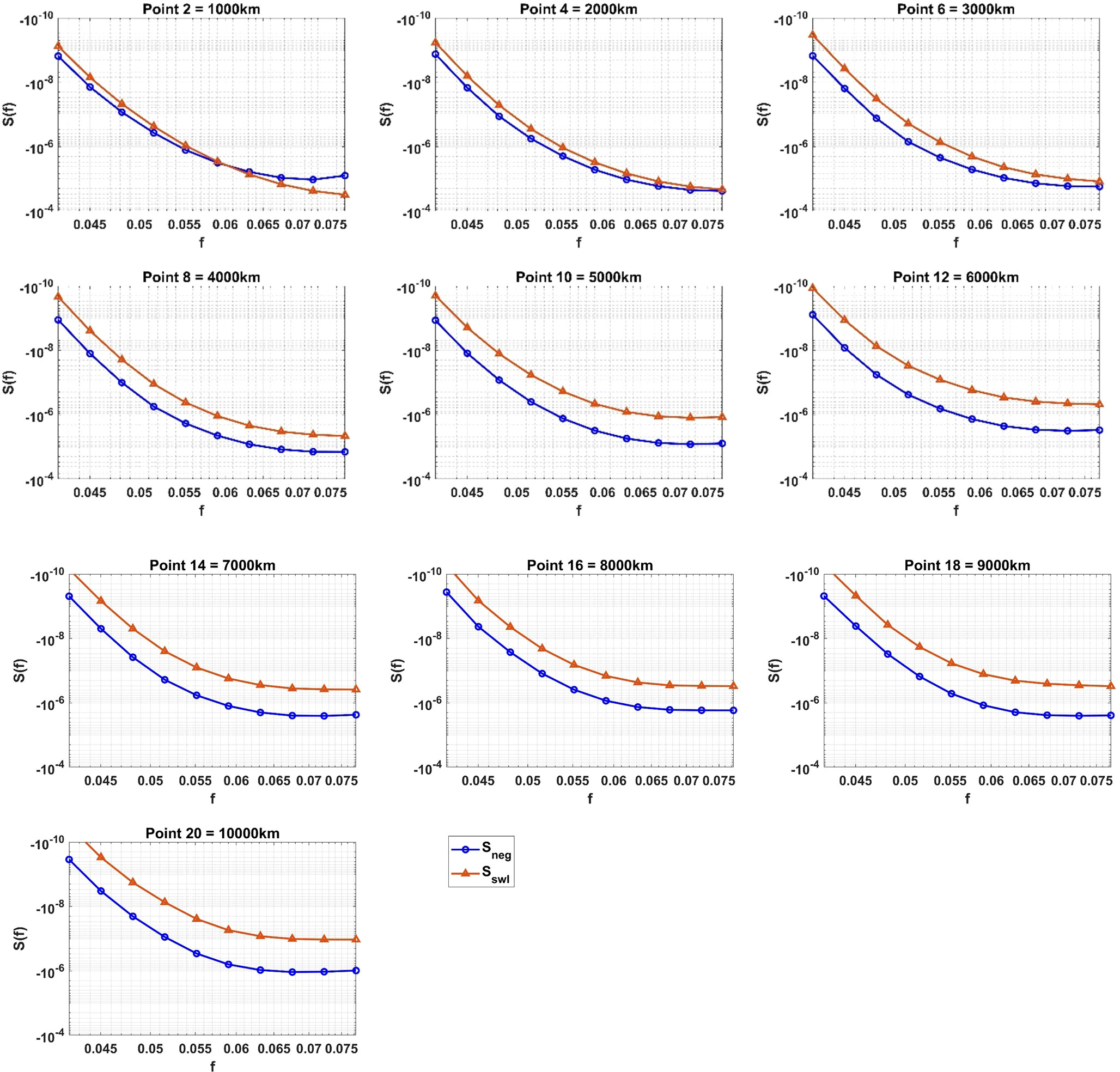
Figure 13 The relative magnitudes of the swell dissipation term, and the negative wind input () averaged over the 4-year period for swell path 8. Each subplot relates to points spaced 1,000 km (every second point) apart along the swell path (see Figure 4). The units of the source terms are [m2/rad].
Noting the relative magnitudes of and , a further test was undertaken with the negative input scaling coefficient, in Equation (13) reduced to a value of 0.05, approximately half its original value.
6.2 Test run results
Figure 14 shows values of the relative normalized bias along each swell path for the original ST6 formulation, the three test runs discussed in Section 6.1 and the standard ST4 run. The color and the size of the markers are proportional to the relative normalized bias values. Note that each of these changes to the source terms will have some impact on the model performance at Campbell Island and no attempt has been made to re-tune the model at this location. Rather, as we use the relative normalized bias by subtracting values of the bias at point 1 along each great circle, these differences in the swell generation region are removed.

Figure 14 Values of relative normalized bias along the 19 Great Circle swell paths for the 5 cases of: (A) Original ST6 case, (B) Test 1 - halved value of in the swell dissipation term, , (C) Test 2 - dependence on wave steepness squared in swell dissipation term, , (D) Test 3 - value of a0 reduced to 0.05 in negative wind term, , (E) Standard ST4 run.
As can be seen from Figure 14, the ST6 and ST4 source term package results are very similar. This is perhaps, not surprising, as both models have been tuned against buoy and altimeter data to model the overall significant wave height optimally. Neither package, however, was tuned to optimally model the swell portion of the spectrum, as investigated here. Therefore, the relatively large biases reported here are not just an artifact of the ST6 package.
Test 1 halved the value of in the swell dissipation term, , and, as seen in Figure 14B, this results in only a relatively small reduction in the relative normalized bias values along each path. In Test 2, the dependence on wave steepness was increased by including a squared dependence on wave slope in swell dissipation term, . As expected (Figure 14C), this further reduces the bias values, with a greater reduction at longer swell propagation distances. In Test 3, the value of was reduced to 0.05 in the negative wind input term, . This change has the largest impact (Figure 14D), with values of bias being significantly reduced at all points except those in the vicinity of the central Pacific Islands and close to the shoreline of Central and South America.
Figure 15 shows the relative normalized bias for the five cases considered along swell path 14, which travels south of the Pacific Islands towards Central America. The original ST6 run has less bias compared to ST4 at shorter propagation distances but larger bias at longer propagation distances. As noted above, this is probably a result of the stronger negative wind input term in the ST6 package. As noted in Figure 14, the absolute values of bias gradually decrease for Test cases 1 and 2, respectively. Test 3, which reduces the negative wind input has the most significant impact, resulting in a flatter bias relationship, which reaches a magnitude of approximately 7% at the longest propagation distances (approx. 8,500km). The bias becomes very large close to the coast of Central and South America. The reason for this is not clear but appears to be a result of either finite depth influences or winds in the region not resolved adequately by the global model and potentially corrupting the swell data.
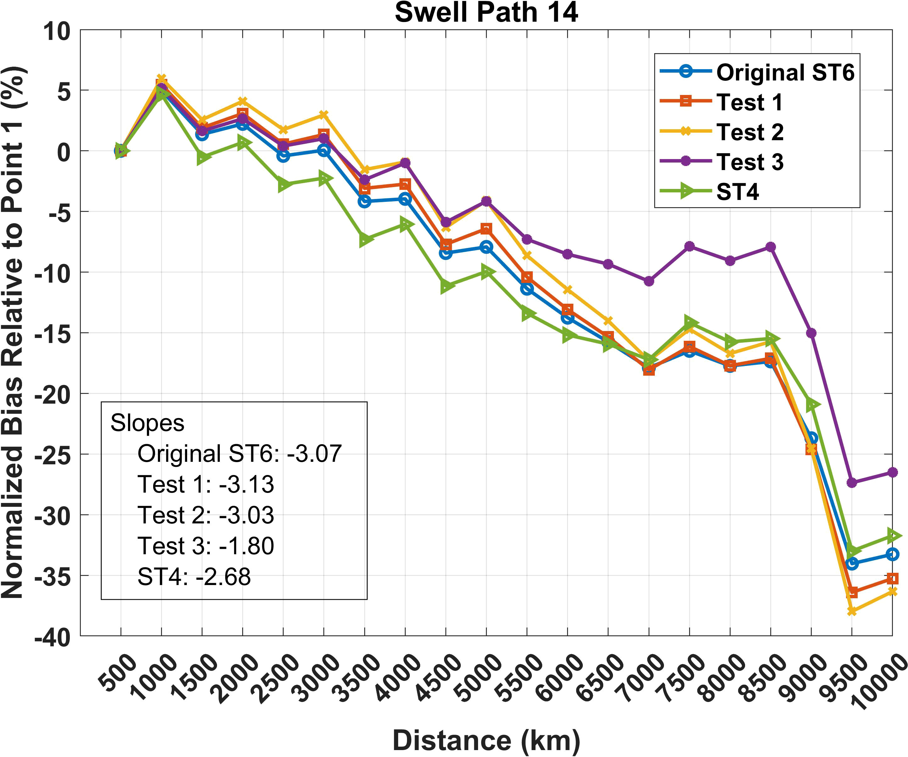
Figure 15 Relative normalized bias for the various tests (Original, ST6, Tests 1 to 3 and ST4) along swell path 14. The slope values for each test were calculated over points 1 to 17.
As a convenient summary diagnostic, the slope of the relative normalized bias as a function of distance (units percent/1000km) for each of the 19 swell paths was calculated for each of the test cases. These values are shown in Table 3. Due to the impact of the coastlines and islands such as Galapagos for points 18 - 20, the slope of each path was calculated over points 1 – 17. The individual slope values for each swell path and the average slope value for each scenario clearly show the relative impact of each test, with Tests 1 and 2 not showing any significant improvement in the performance of the model in reproducing the observed swell decay. The largest improvement, however, occurs in Test 3, as a result of the reduction in the negative wind input. These results suggest that this term in the ST6 package requires further consideration. The results also clearly show that both swell decay and negative wind input terms in contemporary wave models are largely “tuning” terms and, when compared to data of swell decay show significant bias.
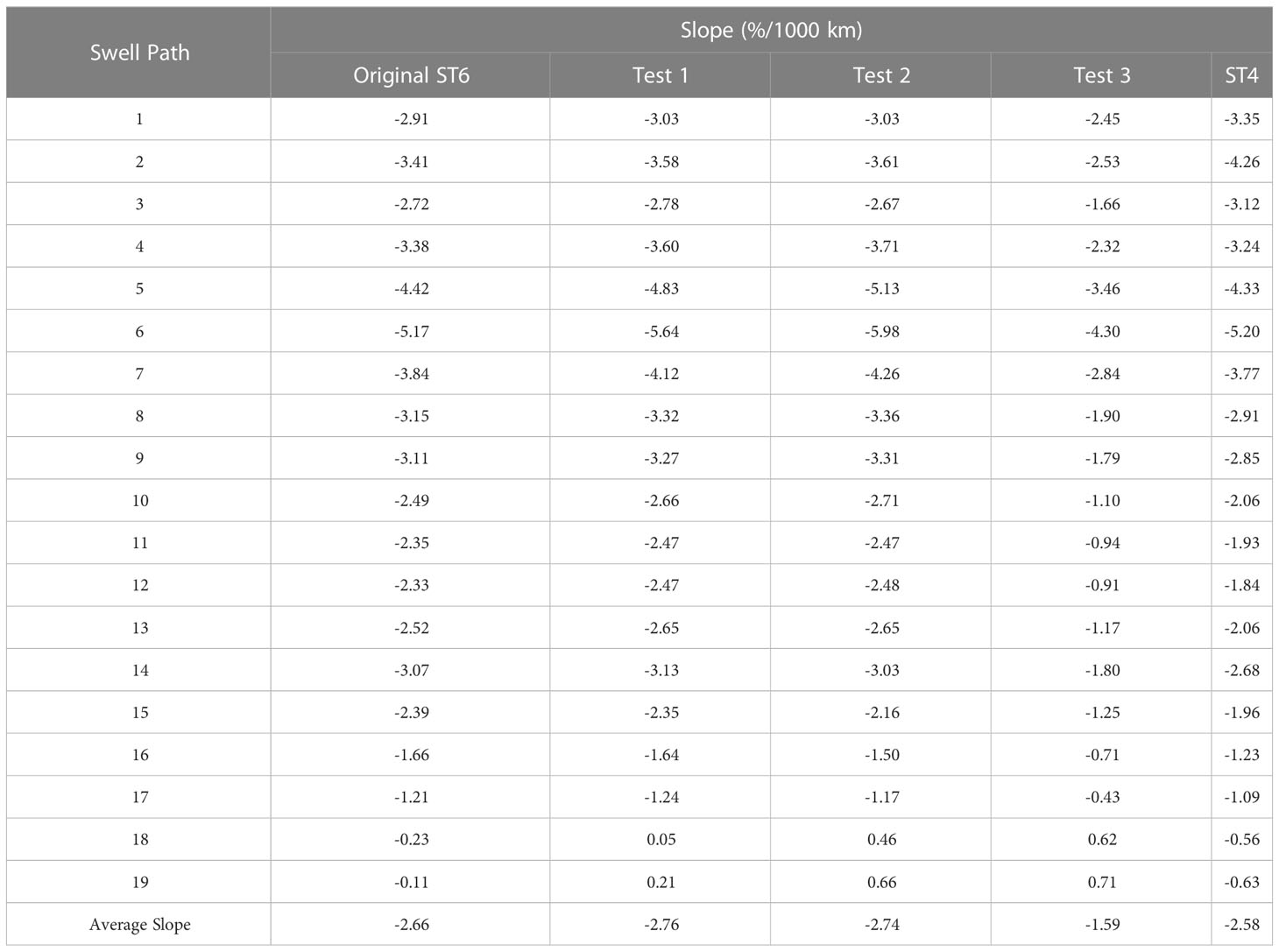
Table 3 Slope value of the 19 swell paths.
In the ST6 package, the negative wind input ( ) and the swell coefficient ( ) have been balanced to obtain an acceptable overall bias and RMS error (Zieger et al., 2015). Although global model validations (Liu et al., 2021) indicate that this works well in predicting overall bulk parameters, such as and , the above results indicate that the model package does not optimally model swell decay. The same conclusion holds for the ST4 package.
7 Conclusions
In this study, swells generated in the region of Campbell Island in the Southern Ocean and propagating across the Pacific Ocean for the years 2017 – 2020 were studied. Observational data collected through the Sentinel-1 SAR and CFOSAT satellites, in-situ buoy networks and model simulated data from the WAVEWATCH III model were utilized as data sources to determine the magnitude of swell decay.
A new methodology was introduced to identify and track Southern Ocean storm swell events. This was done by selecting peaks in the significant wave height measured and modelled at Campbell Island and filtering the events based on mean wave direction, to select cases where the swell generated, propagated across the Pacific Ocean. The swell tracking was achieved by partitioning the spectra in the frequency band 0 – 0.08Hz and propagating the swell from these events along Great Circle paths. Related data for each storm event were extracted from the Sentinel-1 SAR, CFOSAT and WAVEWATCH III datasets, assuming that the swells propagate at their respective group velocities. Comparing the results extracted from each dataset along the selected Great Circle paths showed that the swell tracking method is able to successfully identify swell events and track them along their propagation paths.
The swell decay coefficients calculated from the relationship proposed by Jiang et al. (2016b) for the Sentinel-1 SAR and CFOSAT dataset lie in the same range as previous studies (Ardhuin et al., 2009; Jiang et al., 2016b; Stopa et al., 2016c). The magnitude of the decay coefficient was shown to increase with the wave steepness which implies that steep swell decay at a faster rate.
In order to investigate the physical processes active in the observed swell decay, the WAVEWATCH III model was used as a diagnostic tool. The model was investigated for both ST6 and ST4 source term packages. Both packages produced very similar results, although both showed a strong negative bias for swell, the bias increasing with propagation distance. This indicated that in their present form, such global models appear to dissipate swell too strongly. A series of tests were performed with the ST6 package in an attempt to understand the key processes responsible for the observed dissipation. Tests in which the overall magnitude and dependence on swell steepness of the swell dissipation term, were altered, had only a small impact on the performance and these changes did not remove the model bias, which increases in magnitude with propagation distance. A further test showed that the negative wind input term, has a significant impact on swell dissipation in the ST6 source term package. In fact, at propagation distances greater than approximately 5,000km, this term is actually larger than the swell dissipation term, .
The observed bias in the swell energy within both ST4 and ST6 source term packages, occurs despite the fact that they have been tuned to reproduce observed significant wave height from buoys and altimeters. Thus, the overall may have little bias but the lower frequency swell components are not represented well. There appears to be no simple remedy to these differences and further research is required to better understand the magnitudes of both and . These deficiencies explain why swell prediction in such models continues to remain problematic.
The tests also investigated the impact of currents on swell propagation, with the results indicating currents have only a small effect compared to other physical processes. The results also indicated that the Pacific islands have a large impact on swell propagation which is not well represented by the WW3 sub-grid scale blocking approach.
Data availability statement
The raw data supporting the conclusions of this article will be made available by the authors, without undue reservation.
Author contributions
SP conducted the detailed data analysis and modelling. AM advised on the model development. IY conceived the project and provided supervision. All authors contributed in preparing the manuscript. All authors contributed to the article and approved the submitted version.
Funding
This research was financially supported by the Australian Research Council through grant DP210100840.
Acknowledgments
The authors would like to thank the University of Melbourne for supporting SP through a University of Melbourne postgraduate student scholarship.
Conflict of interest
The authors declare that the research was conducted in the absence of any commercial or financial relationships that could be construed as a potential conflict of interest.
Publisher’s note
All claims expressed in this article are solely those of the authors and do not necessarily represent those of their affiliated organizations, or those of the publisher, the editors and the reviewers. Any product that may be evaluated in this article, or claim that may be made by its manufacturer, is not guaranteed or endorsed by the publisher.
References
Abdalla S., Bidlot J. (2002). Wind gustiness and air density effects and other key changes to wave model in CY25R1. Tech. Rep. Memomrandum R60. 9/SA/0273. Research Department, ECMWF, Reading, U. K.
Alves J. H. G. M. (2006). Numerical modeling of ocean swell contributions to the global wind-wave climate. Ocean Model. 11 (1-2), 98–122. doi: 10.1016/j.ocemod.2004.11.007
Amores A., Marcos M. (2020). Ocean swells along the global coastlines and their climate projections for the twenty-first century. J. Climate 33 (1), 185–199. doi: 10.1175/jcli-d-19-0216.1
Ardhuin F., Chapron B., Collard F. (2009). Observation of swell dissipation across oceans. Geophysical Res. Lett. 36 (6). doi: 10.1029/2008GL037030
Ardhuin F., Rogers E., Babanin A. V., Filipot J. F., Magne R., Roland A., et al. (2010). Semiempirical dissipation source functions for ocean waves. Part I: Definition, calibration, and validation. J. Phys. Oceanography 40 (9), 1917–1941. doi: 10.1175/2010jpo4324.1
Babanin A. V. (2006). On a wave-induced turbulence and a wave-mixed upper ocean layer. Geophysical Res. Lett. 33 (L20605). doi: 10.1029/2006GL027308
Babanin A. V. (2012). “Swell attenuation due to wave-induced turbulence,” in Proceedings of the ASME 31st International Conference on Ocean, Offshore and Arctic Engineering, Vol. 2. 439–443.
Babanin A. V., Jiang H. Y. (2017). “Ocean swell, how much do we know,” in Proceedings of the ASME 36th International Conference on Ocean, Offshore and Arctic Engineering, Vol. 57656.
Babanin A. V., Rogers W. E., de Camargo R., Doble M., Durrant T., Filchuk K., et al. (2019). Waves and swells in high wind and extreme fetches, measurements in the Southern Ocean. Front. Mar. Sci. 6. doi: 10.3389/fmars.2019.00361
Babanin A. V., Soloviev Y. P. (1987). Parameterization of width of directional energy distributions of wind-generated waves at limited fetches. Izvestiya - Atmospheric Ocean Phys. 23 (8), 645–651.
Barber N. F., Ursell F. (1948). The generation and propagation of ocean waves and swell. Part I. Wave periods and velocities. Philos. Trans. R. Soc. London. Ser. A Math. Phys. Sci. 240, 527–560. doi: 10.1098/rsta.1948.0005
Bi F., Song J., Wu K., Xu Y. (2015). Evaluation of the simulation capability of the WAVEWATCH III model for Pacific Ocean wave. Acta Oceanologica Sin. 34 (9), 43–57. doi: 10.1007/s13131-015-0737-1
Cabral I. S., Young I. R., Toffoli A. (2022). Long-term and seasonal variability of wind and wave extremes in the Arctic Ocean. Front. Mar. Sci. 9, 802022. doi: 10.3389/fmars.2022.802022
Cathles L. M., Okal E. A., MacAyeal D. R. (2009). Seismic observations of sea swell on the floating Ross Ice Shelf, Antarctica. J. Geophysical Res. 114 (F2). doi: 10.1029/2007jf000934
Cavaleri L., Alves J. H. G. M., Ardhuin F., Babanin A., Banner M., Belibassakis K., et al. (2007). Wave modelling – The state of the art. Prog. Oceanography 75 (4), 603–674. doi: 10.1016/j.pocean.2007.05.005
Cavaleri L., Fox-Kemper B., Hemer M. (2012). Wind waves in the coupled climate system. Bull. Am. Meteorological Soc. 93 (11), 1651–1661. doi: 10.1175/BAMS-D-11-00170.1
Centre National d’Etudes Spatiales (2020) SWIM product simplified handbook. Available at: https://www.aviso.altimetry.fr/fileadmin/documents/data/tools/SWIM_simplified_handbook.pdf.
Chawla A., Tolman H. L. (2008). Obstruction grids for spectral wave models. Ocean Model. 22 (1-2), 12–25. doi: 10.1016/j.ocemod.2008.01.003
Chen G., Chapron B., Ezraty R., Vandemark D. (2002). A global view of swell and wind sea climate in the ocean by satellite altimeter and scatterometer. J. Atmospheric Oceanic Technol. 19 (11), 1849–1859. doi: 10.1175/1520-0426(2002)019<1849:AGVOSA>2.0.CO;2
Collard F., Ardhuin F., Chapron B. (2009). Monitoring and analysis of ocean swell fields from space: New methods for routine observations. J. Geophysical Res. 114 (C7). doi: 10.1029/2008jc005215
Donelan M. A. (1999). “Wind-induced growth and attenuation of laboratory waves,” in Wind-Over-Wave-Couplings: Perspectives and Prospects. Eds. Sajjadi S. G., Thomas N. H., Hunt J. C. R. (Clarendon Press), 183–194. doi: 10.1175/JPO2933.1
Donelan M. A., Babanin A. V., Young I. R., Banner M. L. (2006). Wave-Follower Field Measurements of the Wind-Input Spectral Function. Part II_ Parameterization of the Wind Input. J. Phys. oceanography 36 (8), 1672–1689. doi: 10.1175/JPO2933.1
Donelan M. A., Babanin A. V., Young I. R., Banner M. L., McCormick C. (2005). Wave Follower Field Measurements of the Wind-Input Spectral Function. Part I Measurements and Calibrations. J. Atmospheric Oceanic Technol. 22 (7), 799–813. doi: 10.1175/JTECH1725.1
Echevarria E. R., Hemer M. A., Holbrook N. J. (2019). Seasonal variability of the global spectral wind wave climate. J. Geophysical Research: Oceans 124 (4), 2924–2939. doi: 10.1029/2018jc014620
Fairall C. W., Bradley E. F., Hare J. E., Grachev A. A., Edson J. B. (2003). Bulk parameterization of air–sea fluxes: Updates and verification for the COARE algorithm. J. Climate 16 (4), 571–591. doi: 10.1175/1520-0442(2003)016<0571:BPOASF>2.0.CO;2
Grant W. D., Madsen O. S. (1979). Combined wave and current interaction with a rough bottom. J. Geophysical Research: Oceans 84 (C4), 1797–1808. doi: 10.1029/JC084iC04p01797
Grelier T., Amiot T., Tison C., Delaye L., Hauser D., Castillan P. (2016). “The SWIM instrument, A wave scatterometer on CFOSAT mission,” in 2016 IEEE International Geoscience and Remote Sensing Symposium (IGARSS). 5793–5796.
Hanley K. E., Belcher S. E., Sullivan P. P. (2010). A global climatology of wind–wave interaction. J. Phys. Oceanography 40 (6), 1263–1282. doi: 10.1175/2010jpo4377.1
Harley M. D., Turner I. L., Kinsela M. A., Middleton J. H., Mumford P. J., Splinter K. D., et al. (2017). Extreme coastal erosion enhanced by anomalous extratropical storm wave direction. Sci. Rep. 7 (1), 1–9. doi: 10.1038/s41598-017-05792-1
Hasselmann S., Hasselmann K., Allender J. H., Barnett T. P. (1985). Computations and Parameterizations of the Nonlinear Energy Transfer in a Gravity-Wave Specturm. Part II Parameterizations of the Nonlinear Energy Transfer for Application in Wave Models. J. Phys. Oceanography 15 (11), 1378–1391. doi: 10.1175/1520-0485(1985)015<1378:CAPOTN>2.0.CO;2
Hauser D., Tison C., Amiot T., Delaye L., Corcoral N., Castillan P. (2017). SWIM: The first spaceborne wave scatterometer. IEEE Trans. Geosci. Remote Sensing Institute Electrical Electron. Engineers 55 (5), 3000–3014. doi: 10.1109/TGRS.2017.2658672
Hauser D., Tourain C., Hermozo L., Alraddawi D., Aouf L., Chapron B., et al. (2021). New Observations From the SWIM Radar On-Board CFOSAT: Instrument Validation and Ocean Wave Measurement Assessment. IEEE Trans. Geosci. Remote Sens. 59 (1), 5–26. doi: 10.1109/TGRS.2020.2994372
Heimbach P., Hasselmann K. (2000). “Development and application of satellite retrievals of ocean wave spectra,” in Elsevier Oceanography Series (Elsevier), 5–33.
Hoeke K., McInnes K. L., Kruger J. C., McNaught R. J., Hunter J. R., Smithers S. G. (2013). Widespread inundation of Pacific islands triggered by distant-source wind-waves. Global Planetary Change 108, 128–138. doi: 10.1016/j.gloplacha.2013.06.006
Högström U., Rutgersson A., Sahlée E., Smedman A. S., Hristov T. S., Drennan W. M., et al. (2012). Air–sea interaction features in the Baltic sea and at a Pacific trade-wind site: An inter-comparison study. Boundary-Layer Meteorology 147 (1), 139–163. doi: 10.1007/s10546-012-9776-8
Holt B., Liu A. K., Wang D. W., Gnanadesikan A., Chen H. S. (1998). Tracking storm-generated waves in the Northeast Pacific Ocean with ERS-1 Synthetic Aperture Radar imagery and buoys. J. Geophysical Research: Oceans 103 (C4), 7917–7929. doi: 10.1029/97jc02567
Janssen P. A. E. M. (1982). Quasilinear approximation for the spectrum of wind-generated water waves. J. Fluid Mechanics 117, 493–506. doi: 10.1017/S0022112082001736
Janssen P. A. (1991). Quasi-linear theory of wind-wave generation applied to wave forecasting. J. Phys. Oceanography 21 (11), 1631–1642. doi: 10.1175/1520-0485(1991)021<1631:QLTOWW>2.0.CO;2
Jiang H., Babanin A. V., Chen G. (2016a). Event-based validation of swell arrival time. J. Phys. Oceanography 46 (12), 3563–3569. doi: 10.1175/jpo-d-16-0208.1
Jiang H., Stopa J. E., Wang H., Husson R., Mouche A., Chapron B., et al. (2016b). Tracking the attenuation and nonbreaking dissipation of swells using altimeters. J. Geophysical Research: Oceans 121 (2), 1446–1458. doi: 10.1002/2015jc011536
Khan S. S., Echevarria E. R., Hemer M. A. (2021). Ocean swell comparisons between Sentinel-1 and WAVEWATCH III around Australia. J. Geophysical Research: Oceans 126 (2). doi: 10.1029/2020jc016265
Komen G. J., Cavaleri L., Donelan M., Hasselmann K., Hasselmann S., Janssen P. A. E. M. (1994). Dynamics and modelling of ocean waves (Cambridge University Press). 532pp.
Komen G. J., Hasselmann S., Hasselmann K. (1984). On the existence of a fully developed wind-sea spectrum. J. Phys. Oceanography 14 (8), 1271–1285. doi: 10.1175/1520-0485(1984)014<1271:OTEOAF>2.0.CO;2
Lefèvre J. M. (2008). High swell warnings in the Caribbean Islands during March 2008. Natural Hazards 49 (2), 361–370. doi: 10.1007/s11069-008-9323-6
Le Merle E., Hauser D., Peureux C., Aouf L., Schippers P., Dufour C., et al. (2021). Directional and Frequency Spread of Surface Ocean Waves From SWIM Measurements. J. Geophysical Research: Oceans 126 (7). doi: 10.1029/2021jc017220
Liu Q., Babanin A. V., Rogers W. E., Zieger S., Young I. R., Bidlot J. R., et al. (2021). Global Wave Hindcasts Using the Observation-Based Source Terms: Description and Validation. J. Adv. Modeling Earth Syst. 13 (8). doi: 10.1029/2021ms002493
Liu Q., Rogers W. E., Babanin A. V., Young I. R., Romero L., Zieger S., et al. (2019). Observation-based source terms in the third-generation wave model WAVEWATCH III: Updates and verification. J. Phys. Oceanography 49 (2), 489–517. doi: 10.1175/jpo-d-18-0137.1
McComb P., Garrett S., Durrant T., Perez J. (2021). Directional wave buoy data measured near Campbell Island, New Zealand. Sci. Data 8 (1), 239. doi: 10.1038/s41597-021-01025-3
Mentaschi L., Kakoulaki G., Vousdoukas M., Voukouvalas E., Feyen L., Besio G. (2018). Parameterizing unresolved obstacles with source terms in wave modeling: A real-world application. Ocean Model. 126, 77–84. doi: 10.1016/j.ocemod.2018.04.003
Meucci A., Young I. R., Hemer M., Trenham C., Watterson I. G. (2023). 140 years of global ocean wind-wave climate derived from CMIP6 ACCESS-CM2 and EC-Earth3 GCMs: Global trends, regional changes, and future projections. J. Climate 36 (6), 1605–1631. doi: 10.1175/JCLI-D-21-0929.1
Miles J. W. (1957). On the generation of surface waves by shear flows. J. Fluid Mechanics 3 (2), 185–204. doi: 10.1017/S0022112057000567
Munk W. H. (1947). Tracking Storms by Forerunners of Swell. J. Atmospheric Sci. 4 (2), 45–57. doi: 10.1175/1520-0469(1947)004<0045:TSBFOS>2.0.CO;2
Munk W. H., Miller G. R., Snodgrass F. E., Barber N. F. (1963). Directional recording of swell from distant storms. Philos. Trans. R. Soc. London. Ser. A Math. Phys. Sci. 255 (1062), 505–584. doi: 10.1098/rsta.1963.0011
Palmer T., Nicholls R. J., Wells N. C., Saulter A., Mason T. (2014). Identification of ‘energetic’ swell waves in a tidal strait. Continental Shelf Res. 88, 203–215. doi: 10.1016/j.csr.2014.08.004
Phillips O. M. (1977). The dynamics of the upper ocean (New York: Cambridge University Press). 336pp.
Portilla J. (2012). Storm-source-locating algorithm based on the dispersive nature of ocean swells. Avances-USFQ 4 (1), C22–C36.
Rapley C. G. (1984). First observations of the interaction of ocean swell with sea ice using radar altimeter data. Nature 307 (5947), 150–152. doi: 10.1038/307150a0
Rascle N., Ardhuin F. (2013). A global wave parameter database for geophysical applications. Part 2: Model validation with improved source term parameterization. Ocean Model. 70, 174–188. doi: 10.1016/j.ocemod.2012.12.001
Rascle N., Ardhuin F., Queffeulou P., Croizé-Fillon D. (2008). A global wave parameter database for geophysical applications. Part 1: Wave-current–turbulence interaction parameters for the open ocean based on traditional parameterizations. Ocean Model. 25 (3-4), 154–171. doi: 10.1016/j.ocemod.2008.07.006
Ribal A., Young I. R. (2019). 33 years of globally calibrated wave height and wind speed data based on altimeter observations. Sci. Data 6 (1), 77. doi: 10.1038/s41597-019-0083-9
Rogers W. E. (2002). The US Navy's global wind-wave models: An investigation into sources of errors in low-frequency energy predictions. Tech. Report Oceanography Division Naval Res. Laboratory Stennis Space Center, 7320–02-10035.
Rogers W. E., Babanin A. V., Wang D. W. (2012). Observation-consistent input and whitecapping dissipation in a model for wind-generated surface waves: Description and simple calculations. J. Atmospheric Oceanic Technol. 29 (9), 1329–1346. doi: 10.1175/JTECH-D-11-00092.1
Rogers W. E., Hwang P. A., Wang D. W. (2003). Investigation of wave growth and decay in the SWAN model: Three regional-scale applications. J. Phys. Oceanography 33 (2), 366–389. doi: 10.1175/1520-0485(2003)033<0366:IOWGAD>2.0.CO;2
Semedo A., Sušelj K., Rutgersson A., Sterl A. (2011). A global view on the wind sea and swell climate and variability from ERA-40. J. Climate 24 (5), 1461–1479. doi: 10.1175/2010jcli3718.1
Smith G. A., Hemer M., Greenslade D., Trenham C., Zieger S., Durrant T. (2021). Global wave hindcast with Australian and Pacific Island focus: From past to present. Geosci. Data J. 8 (1), 24–33. doi: 10.1002/gdj3.104
Snodgrass F. E., Groves G. W., Hasselmann K. F., Miller G. R., Munk W. H., Powers W. H. (1966). Propagation of ocean swell across the Pacific. Philos. Trans. R. Soc. London. Ser. A Math. Phys. Sci. 259 (1103), 431–497. doi: 10.1098/rsta.1966.0022
Soran M. B., Amarouche K., Akpınar A. (2022). Spatial calibration of WAVEWATCH III model against satellite observations using different input and dissipation parameterizations in the Black Sea. Ocean Eng. 257, 111627. doi: 10.1016/j.oceaneng.2022.111627
Stopa J. E. (2018). Wind forcing calibration and wave hindcast comparison using multiple reanalysis and merged satellite wind datasets. Ocean Model. 127, 55–69. doi: 10.1016/j.ocemod.2018.04.008
Stopa J. E., Ardhuin F., Babanin A., Zieger S. (2016a). Comparison and validation of physical wave parameterizations in spectral wave models. Ocean Model. 103, 2–17. doi: 10.1016/j.ocemod.2015.09.003
Stopa J. E., Ardhuin F., Girard-Ardhuin F. (2016b). Wave climate in the Arctic 1992–2014: seasonality and trends. Cryosphere 10 (4), 1605–1629. doi: 10.5194/tc-10-1605-2016
Stopa J. E., Ardhuin F., Husson R., Jiang H., Chapron B., Collard F. (2016c). Swell dissipation from 10 years of Envisat Advanced Synthetic Aperture Radar in wave mode. Geophysical Res. Lett. 43 (7), 3423–3430. doi: 10.1002/2015GL067566
Tison C., Hauser D. (2018). "Swim products users guide: Product description and algorithm theoretical baseline description" (Toulouse). Available at: https://www.aviso.altimetry.fr/fileadmin/documents/data/tools/SWIM_ProductUserGuide.pdf.
Tolman H. L. (1990). The influence of unsteady depths and currents of tides on wind-wave propagation in shelf seas. J. Phys. Oceanography 20 (8), 1166–1174. doi: 10.1175/1520-0485(1990)020<1166:TIOUDA>2.0.CO;2
Tolman H. L. (2002). Alleviating the garden sprinkler effect in wind wave models. Ocean Modeling 4, 269–289. doi: 10.1016/S1463-5003(02)00004-5
Tolman H. L., Chalikov D. (1996). Source terms in a third-generation wind wave model. J. Phys. Oceanography 26 (11), 2497–2518. doi: 10.1175/1520-0485(1996)026<2497:STIATG>2.0.CO;2
Umesh P. A., Behera M. R. (2020). Performance evaluation of input-dissipation parameterizations in WAVEWATCH III and comparison of wave hindcast with nested WAVEWATCH III-SWAN in the Indian Seas. Ocean Eng. 202, 106959. doi: 10.1016/j.oceaneng.2020.106959
WAMDI (1988). The WAM model—A third generation ocean wave prediction model. J. Phys. Oceanography 18 (12), 1775–1810.
Wang X., Jiang H., Chen G., Yu F. (2016). Identifying storm-induced wave origins using SAR wave mode data. Sci. China Earth Sci. 59 (10), 1971–1980. doi: 10.1007/s11430-015-5478-3
Wiegel R. L. (1960). Wind waves and swell. Proc. Seventh Conf. Coast. Eng. 7), 1–40. doi: 10.9753/icce.v7.1
Williams G., Buchan S. (2015). “Advances in swell prediction for Australia’s North West shelf,” in 14th International Workshop on Wave Hindcasting and Forecasting and 5th Coastal Hazard Symposium.
Wingeart K. M., Herbers T. H., O'Reilly W. C., Wittmann P. A., Jensen R. E., Tolman H. L. (2002). Validation of operational global wave prediction models with spectral buoy data. Ocean Wave Measurement Anal. 2001, 590–599. doi: 10.1061/40604(273)61
WW3DG, T.W.I.D.G (2019). User manual and system documentation of WAVEWATCH III R version 6.07 (MD, USA: NOAA/NWS/NCEP/MMAB, College Park).
Young I. R., Babanin A. V., Zieger S. (2013). The decay rate of ocean swell observed by altimeter. J. Phys. Oceanography 43 (11), 2322–2333. doi: 10.1175/jpo-d-13-083.1
Young I. R., Banner M. L., Donelan M. A., McCormick C., Babanin A. V., Melville W. K., et al. (2005). An integrated system for the study of wind-wave source terms in finite-depth water. J. Atmospheric Oceanic Technol. 22 (7), 814–831. doi: 10.1175/JTECH1726.1
Young I. R., Fontaine E., Liu Q., Babanin A. V. (2020). The wave climate of the Southern Ocean. J. Phys. Oceanography 50 (5), 1417–1433. doi: 10.1175/jpo-d-20-0031.1
Young I. R., Sobey R. J. (1985). Measurements of the wind-wave energy flux in an opposing wind. J. Fluid Mechanics 151, 427–442. doi: 10.1017/s0022112085001033
Young I. R., Sobey R. J. (1988). Deep water swell and spectral wave decay in opposing winds. J. Waterway Port Coastal Ocean Eng. 114 (6), 732–744. doi: 10.1061/(asce)0733-950x(1988)114:6(732
Zaug C. R., Carter J. D. (2021). Dissipative models of swell propagation across the Pacific. Stud. Appl. Mathematics 147 (4), 1519–1537. doi: 10.1111/sapm.12423
Keywords: Ocean swell, WAVEWATCH III, wave modelling, swell dissipation, sentinel-1 SAR, negative wind input
Citation: Pathirana S, Young I and Meucci A (2023) Modelling swell propagation across the Pacific. Front. Mar. Sci. 10:1187473. doi: 10.3389/fmars.2023.1187473
Received: 16 March 2023; Accepted: 06 July 2023;
Published: 24 July 2023.
Edited by:
Jingsong Yang, Ministry of Natural Resources, ChinaReviewed by:
Yukiharu Hisaki, University of the Ryukyus, JapanJohn Carter, Seattle University, United States
Kejian Wu, Ocean University of China, China
Copyright © 2023 Pathirana, Young and Meucci. This is an open-access article distributed under the terms of the Creative Commons Attribution License (CC BY). The use, distribution or reproduction in other forums is permitted, provided the original author(s) and the copyright owner(s) are credited and that the original publication in this journal is cited, in accordance with accepted academic practice. No use, distribution or reproduction is permitted which does not comply with these terms.
*Correspondence: Ian Young, aWFuLnlvdW5nQHVuaW1lbGIuZWR1LmF1