 Ramin Familkhalili
 Jenny Davis
 Carolyn A. Currin
 Madison E. Heppe
 Susan Cohen
- 1National Centers for Coastal Ocean Science, National Oceanic and Atmospheric Administration, Beaufort, NC, United States
- 2Consolidated Safety Services, Inc., Fairfax, VA, United States
- 3EA Engineering, Science, and Technology, Inc., PBC, Hunt Valley, MD, United States
- 4Institute for the Environment, University of North Carolina at Chapel Hill, Chapel Hill, NC, United States
The capacity of vegetated coastal habitats to mitigate erosion and build elevation in response to sea-level rise (SLR) has led to growing interest in their application as Nature Based Solutions (NBS) for shoreline protection. However, a significant uncertainty in the performance of NBS is how these features will respond to future rates of SLR. In this study, we applied the Sea Level Affecting Marshes Model (SLAMM) to a fringing shoreline wetland complex that is directly adjacent to the primary runway of a regional airport in coastal North Carolina, US. The SLAMM model was run at high spatial resolution (1 m cell size) to investigate the effects of projected SLR by 2100 on the wetland communities and to estimate the potential benefits of a proposed NBS project involving the use of dredged sediment to increase wetland surface elevation. Modeling future habitat extent under three SLR scenarios (i.e., intermediate, intermediate-high, and high) with no land modification reveals a consistent pattern of salt marsh expanding into fresh marsh, salt marsh transitioning to higher elevations, and substantially larger overall extents of intertidal and subtidal habitats within the project footprint at relatively high rates of SLR. Simulations that include the NBS indicate changes in the composition of wetland types over time compared with the no-action scenario. Model results help to better understand the long-term behavior of fringing coastal wetlands and the efficacy of their use as part of coastal resilience strategies.
1 Introduction
Fringing coastal wetlands are common along estuarine shorelines of the Southeastern US. These narrow bands of wetland are a vital transition zone between land and water and are highly dynamic environments that are influenced by both natural and anthropogenic factors including accelerating rates of SLR, wind-induced wave erosion, altered sediment supply, boat wakes, land-use changes, and manmade urban development (e.g., Gilby et al., 2021). The traditional approach to protecting coastal shorelines from these hazards has involved shoreline hardening (e.g., seawalls, revetments, and bulkheads), also known as “hard” or “gray” structures (e.g., Dugan et al., 2011; Polk et al., 2022). In the US, almost 14% of the estuarine shoreline has been hardened to maintain the shoreline position (Gittman et al., 2015). These gray shoreline protection structures, which are generally installed at the transition between coastal wetland and uplands, interrupt the estuarine shoreline’s natural function by altering sediment transport and deposition (e.g., Kirwan and Murray, 2008; Currin, 2019) and impeding wetland migration (e.g., Spencer et al., 2016). In addition, the wave energy that reflects off of hard structures, can lead to increased erosion of marsh seaward of the structure and shoreline adjacent to the structure (e.g., Bozek and Burdick, 2005; Bendoni et al., 2016).
There are many benefits associated with natural coastal wetland habitats, including protecting against erosion and storm impacts (e.g., Temmerman et al., 2013; Möller et al., 2014), sequestering carbon (e.g., Kirwan and Guntenspergen, 2012; Duarte et al., 2013), providing habitat for wildlife (e.g., Bilkovic et al., 2006), and improving water quality by trapping coastal sediments and sequestering nutrients. Furthermore, it has been estimated that the ecosystem services (such as food control, climate regulation, natural hazard mitigation, water purification, and soil formation) provided by coastal wetlands worldwide are valued at ~$194,000 per hectare per year, while wetland protection against floods and storms could have a yearly benefit of $23 billion to coastal communities in the US (Costanza et al., 2008; Costanza et al., 2014). Wetlands also saved ~$625 million in direct flood damage from Hurricane Sandy (Narayan et al., 2017). Growing recognition of the value of intact natural habitats for shoreline protection has fueled an interest in their use as NBS to coastal hazards (e.g., Gittman et al., 2016; Smith et al., 2020). NBS practices involve the use of natural habitats either alone or in combination with man-made structures to mitigate erosion and preserve valuable shoreline habitats (e.g., Arkema et al., 2013). One of the major impediments to widespread acceptance of NBS practices is uncertainty about how these sites will change overtime as they mature and adapt to environmental stressors like SLR (Möller, 2019).
The impacts of SLR on the environment have been identified in a variety of studies as one of the most certain and potentially destructive effects of climate change (e.g., IPCC, 2007). Similarly, coastal wetlands are threatened by global climate change, land loss, and anthropogenic activities, and their long-term sustainability depends on sediment delivery and biological productivity (e.g., Nicholls et al., 2007; Karl et al., 2009). Satellite imagery analysis revealed that there has been ~360,000 acres of global salt marsh loss between 2000 and 2019 (Campbell et al., 2022) and within the US alone, ~62,300 acres of wetland lost between 2004 and 2009 due to erosion, land subsidence, SLR, and human activities (Dahl, 2011). It is estimated that 20–60% of the world’s coastal wetlands could be submerged as a result of SLR by the end of the 21st century (e.g., Nicholls et al., 2007; Craft et al., 2009) and if greenhouse gas emissions are not mitigated, this loss could exceed 90% which would convert productive tidal marshes to subtidal habitats (Crosby et al., 2016). The susceptibility of coastal habitats to climate change-induced SLR naturally calls into question the efficacy of using NBS approaches for shoreline stabilization.
In this study, we quantify the impacts of projected SLR scenarios on the evolution of coastal wetlands around the Michael J. Smith Field Airport (NC) - a strategic infrastructure in the area - by developing a numerical model (SLAMM). We further use SLAMM to investigate the effects of implementing an NBS project that involves the use of dredged sediments and shore parallel sills to restore and sustain wetlands. We simulate the transformation of coastal environments in response to long-term SLR and beneficially used dredged sediments by accounting for nearshore geomorphological processes such as accretion, erosion, and marsh migration. SLAMM uses a simple framework and simulates the main processes involved in wetland conversions, habitat, and shoreline changes to evaluate potential changes in the distribution and extent of marshlands (see SLAMM technical documentation).
We first provide a brief overview of the marshland area and describe in detail the morphological changes, both natural and manmade, observed during the last 60-70 years. We then outline the main features of the numerical model employed in this study, together with a description of the model input used. Finally, we report the results of the model simulations and discuss in detail the findings of this investigation. This study helps to build bridges from fundamental research to engineering applications with environmental and societal benefits. The approach and results of this study could be used to plan for the management of coastal wetland systems in the context of SLR.
2 Study area
North Carolina, located in the mid-Atlantic region of the US (Figure 1A), has ~12000 miles of estuarine shoreline, much of which is characterized by intertidal salt marsh communities that provide critical habitat for a wide range of plant and animal species. Our project area includes the nearshore subtidal, intertidal fringing marsh system, and low elevation upland regions adjacent to Michael J. Smith Field Airport in Beaufort, NC (Figure 1B) that serves as key regional infrastructure. The airport upland regions and adjacent open water are separated by a narrow band of marsh, and the marsh shoreline has receded at an average rate of 0.62 m/yr over the past 60 years (see blue and red lines in Figure 1B). Continuous losses of this magnitude threaten the runways’ long-term stability. Additionally, runways hinder inland marsh migration, so restoring the marsh by raising the elevation of the marsh platform and building seaward sills to counter historical losses is one of the few NBS strategies available to promote marsh persistence without migration.
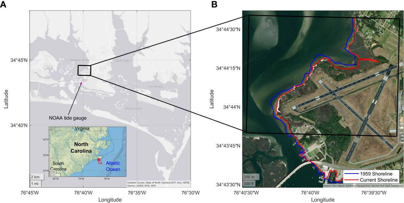
Figure 1 (A) The project area is within the Newport River estuary on the central coast of North Carolina and (B) The model domain is restricted to the intertidal region directly adjacent to the Michael J. Smith Field Airport. Blue line is the digitized shoreline position in 1959 and the red line in 2022.
The nearest available NOAA long-term tide gauge (National Water Level Observation Network, NWLON#8656483) is within 1 mile of the project site (Figure 1A). A comparison of the historic 1959 and current shorelines (i.e., water-land boundary position) obtained from aerial imagery (Figure 1B) was used to calculate erosion rates (see Sec 3.5). Ground-based surveys were conducted to determine the elevation tolerances of the existing wetland plant communities and to ground truth the accuracy of available LiDAR-generated digital elevation models of the area. These data provided the basis for design of a restoration project that would restore the marsh footprint to its 1959 extent with a NBS using sediments dredged from the nearby Atlantic Intracoastal Waterway. The modeling effort described here is intended to evaluate the impact of this project, should it be implemented, on the future evolution of this critical shoreline habitat.
3 Methods and data
We applied SLAMM to predict the wetland landscape in 2100 using two starting scenarios: 1) baseline conditions (reflecting the current distribution of shoreline habitats) and 2) restored conditions, using the restoration design described above (see also Sec 5 for details). SLAMM has been widely used to estimate the impacts of SLR on wetlands (e.g., Craft et al., 2009; Glick et al., 2013; Clough et al., 2016). Using SLAMM, we can assess the extent to which seawater inundation contributes to the conversion of one wetland type to another based on the land elevation and coverage type, slope, and rates of accretion, sedimentation, and erosion. By reducing the relative elevations of each model cell as water level increases, SLAMM tracks inundation and corresponding rises in the salt boundary (the elevation that defines the transition between salt marsh and upland). The spatial data required for SLAMM include elevation, slope, initial habitat distribution, impervious land, vegetation and soil characteristics (e.g., accretion and erosion rates), tidal datums, and SLR.
3.1 Elevation data
The digital elevation model used here (Figure 2A) to represent current conditions is based on a 1 m Topo-Bathymetric Digital Elevation Model (TBDEM relative to the North American Vertical Datum of 1988, NAVD88) from the Coastal National Elevation Database (CoNED) which consists of both LiDAR and bathymetry data (https://www.usgs.gov/special-topics/coastal-national-elevation-database-applications-project). The LiDAR data cover dry land, wetlands area, and shallow waters (shallower than approximately 0.75 m NAVD88), and the bathymetry data cover the navigation channel and other deep-water regions. SLAMM processes all elevations referenced to Mean Tide Level (MTL) and therefore elevation data were transformed to MTL using the relationships published for the nearby NOAA long-term tide gauge (https://tidesandcurrents.noaa.gov/datums.html?id=8656483). All elevations were < ~5 m above MTL, with 27%, 56%, and 72% of elevations above high, intermediate-high, and intermediate SLR scenarios, respectively (Figure 2B).
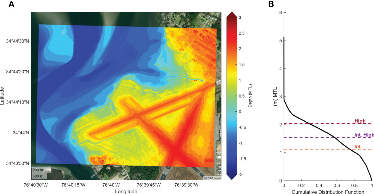
Figure 2 (A) TBDEM of the model domain and (B) Cumulative distribution function of ground elevation above 0-MTL.
In addition to the elevation layer, a slope layer was created. The slope of a TBDEM in degrees is required input data and is calculated by determining the maximum rate of change (rise over run) between an individual cell and its eight neighbors. SLAMM calculates a partial cell conversion based on the slope data, which provides a range of elevations in a cell.
As wetland response to SLR and inundation modeling is particularly dependent on topography (e.g., Mogensen and Rogers, 2018; Alizad et al., 2020), we validated the quality of the TBDEM by comparison with ~2300 real-time kinematic global positioning system (RTK-GPS) elevation measurements collected (vertical accuracy of ±0.02m based on standard error of repeated measures of a reference point) at the site. The RTK-GPS measurements were not used to create a new TBDEM, but only to verify accuracy of the CoNED TBDEM. Based on a high coefficient of determination of 0.94 and root-mean-square error of 0.13 m (Figure 3), the TBDEM is a reasonable representation of the wetland topography. Overall, RTK-measured and TBDEM-modeled elevations differ slightly, likely due to a combination of the georeferencing of the lidar point cloud and the dynamic nature of the sandy berm that exists at the shoreward edge of the marsh on the west-facing shoreline (defined in the model as estuarine beach). In the regularly flooded marsh (i.e., intermediate to high marsh at elevations between 0 and 0.4 NAVD88), the elevation discrepancy is larger due to dense vegetation (see cyan color dots in Figure 3), which results in an overestimate of surface elevation by LiDAR data.
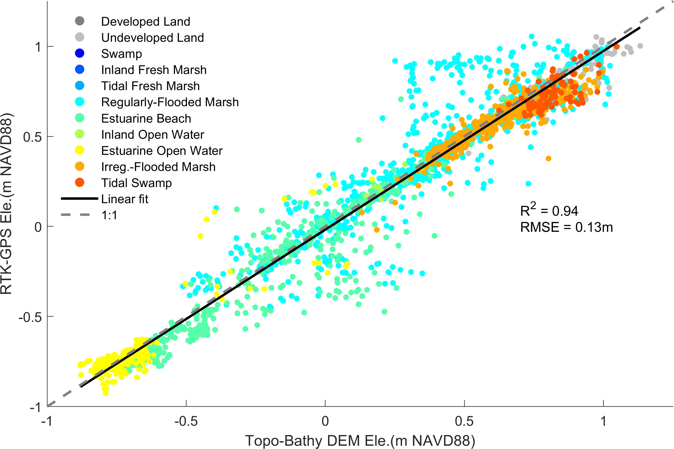
Figure 3 Comparison of RTK-GPS elevation measurements with respective elevation values of the TBDEM. The color coding corresponds to the land/water cover (see Sec 3.2).
3.2 Land and water cover
Land and water cover information were obtained from the 2019 National Wetlands Inventory (NWI) maps of wetlands and deep-water habitats from the US Fish and Wildlife Service (USFWS, https://www.fws.gov/program/national-wetlands-inventory). We also used a high-resolution land cover layer obtained from the Multi-Resolution Land Characteristics Consortium (MRLC; https://www.mrlc.gov) to split dry land into developed and undeveloped categories. To prepare a land/water cover layer for the SLAMM model, we categorized the NWI land-water classifications to 26 SLAMM categories that determine the dominant processes involved in wetland conversions and shoreline modifications (Figure 4, also see SLAMM 6.7 technical documentation for more details). NWI maps were converted from polygon data to raster-based maps with the same spatial resolution as the elevation and slope raster maps (i.e., 1 m cell size). Land and water cover types for the entire 252 ha study area are summarized in Table 1.
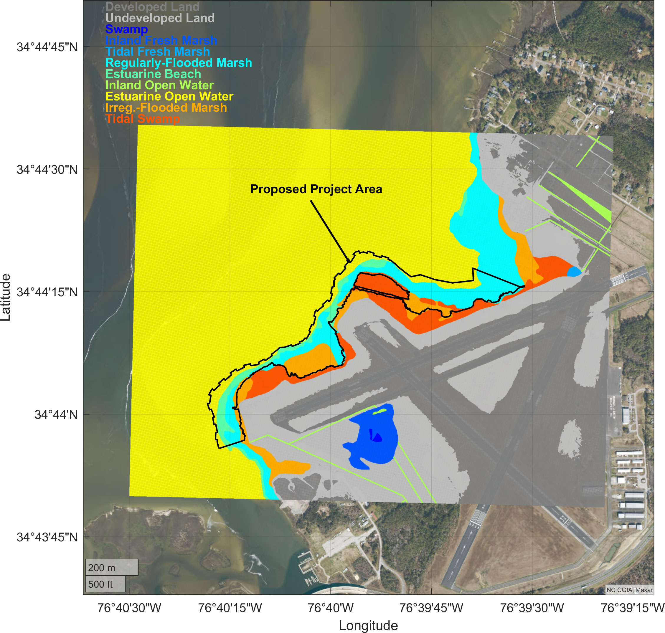
Figure 4 Land and water cover area for SLAMM model.
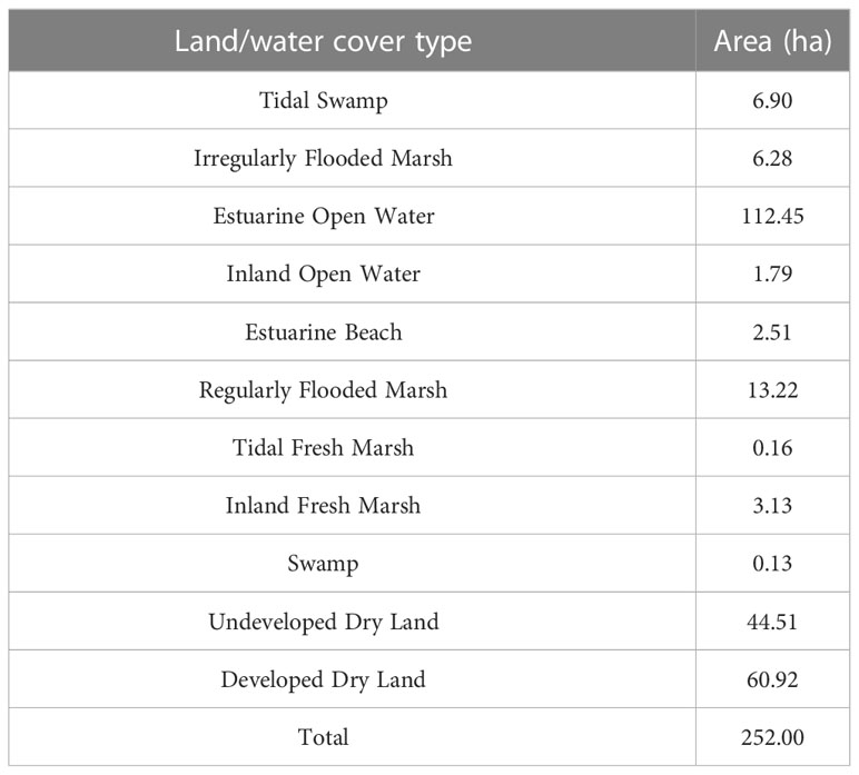
Table 1 Initial condition land/water cover categories for the model domain.
As shown in Table 1, ~42% of the model area is dry land (both developed and undeveloped) and open water covers ~45% of the area. The most prominent wetland types in the model area are regularly flooded marsh (13.22 ha, ~5.25% of model domain), tidal swamp (6.9 ha, ~2.74% of model domain), and irregularly flooded marsh (6.28 ha, ~2.49% of model domain). Other types of wetlands combined comprise less than 3% of the study area. Dry land (developed and undeveloped) areas could be inundated under the projected SLR scenarios used in the model as they are not protected by dikes, levees, or other coastal armoring.
3.3 Tidal datum and mean sea level
The primary tidal datums relative to NAVD88 at the NOAA Beaufort station (Figure 1A) are presented in Table 2. Due to the area of interest being very close to the ocean inlet, it is reasonable to use the oceanic MSL instead of the estuary MSL and thus we derived the MSL from ocean water level records (available from NWLON#8656483).
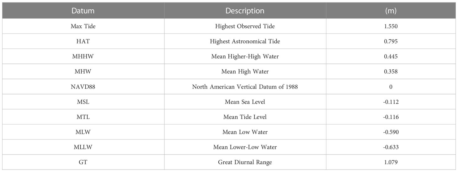
Table 2 Tidal elevation statistics at Beaufort, NC.
Hourly tide data used to calculate tidal variations, mean sea level, and to validate the model were obtained from the NOAA Beaufort NWLON station (data period 1967–2022, Figure 5A). We use the gauge data to calculate both tidal exceedance and salt elevation and to determine model tidal boundary conditions. Tidal datum, present epoch (1983-2001) data, and historic SLR trend data were downloaded from the NOAA NOS/CO-OPS website for Beaufort, NC (NWLON#8656483). The long-term (1967-2022) mean sea-level trend for Beaufort is increasing at 3.4 mm/yr (Figure 5A), while a linear regression analysis over the last 20 years of data indicate a recent rate of 8.6 mm/yr. From the hourly tide records, we extracted the monthly mean high and low tides and the difference was used to calculate mean tidal range, which has been increasing at a rate of 3.04 mm/yr since the 1960s (Figure 5B).
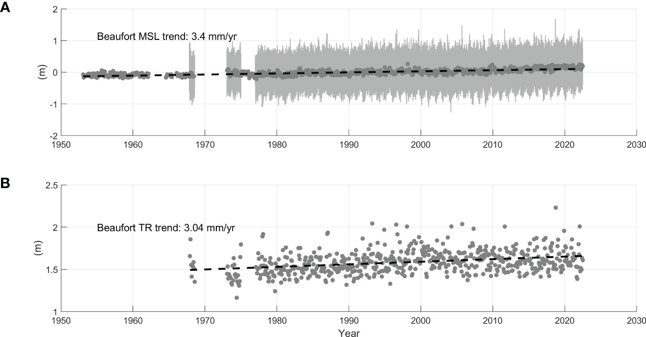
Figure 5 (A) Changes in hourly water level (gray line, 1967-2022) and monthly mean sea level (gray dots 1953-2022) relative to MSL, and (B) Changes in monthly mean tidal range (TR) since the 1960s at Beaufort, NC. Trends were calculated using a robust linear regression (black dash lines) with a standard error of 0.2 mm/yr.
Analyzing historical hourly water level data from the NOAA Beaufort tide gauge provides valuable insights into the frequency and extent of high-water levels in the region. The analysis shows that around 12% of the time, water levels exceed the MHW threshold of 0.47 m-MSL while the majority of the time (approximately 78%), water levels fall between the MLW and MHW thresholds (Figure 6). Based on the data collected through field observations, it has been determined that the elevations of the local coastal wetlands fall within the range of ~-0.04 to 1.18 m-MSL.
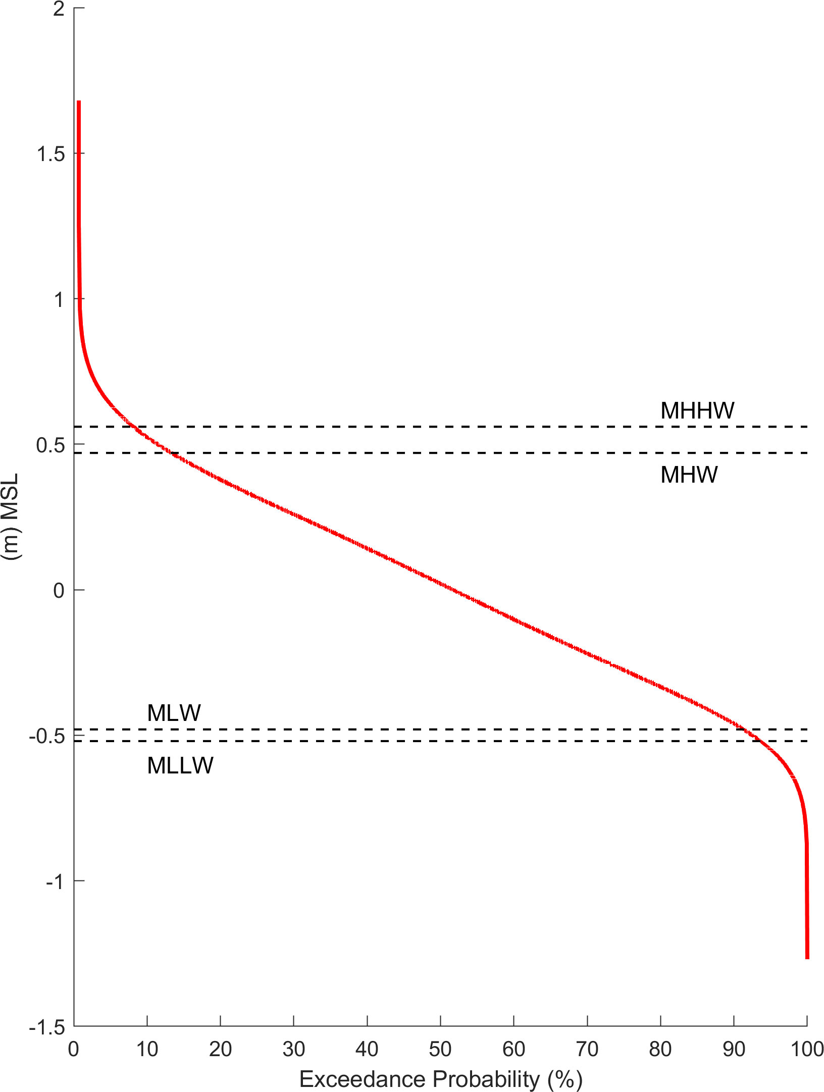
Figure 6 Water-level exceedance probability curve for Beaufort, NC.
3.4 SLR scenarios
The Earth’s average temperature has warmed gradually over the last century, mostly due to human influence of burning of fossil fuels and resulting accumulation of greenhouse gasses in the atmosphere (IPCC, 2012) which resulted in accelerated SLR. SLR is a result of a variety of factors, including thermal expansion of ocean water and increasing freshwater inputs from melting glaciers (Sweet et al., 2022). The global increase by 2100 is predicted to range between 0.3 m and 2.0 m (e.g., Sweet et al., 2022). In addition to global factors, local variations in SLR such as vertical land movement (uplift or subsidence), changing gravitational attraction due to ice masses, and changes in regional ocean circulation (e.g., Nicholls et al., 2014; Valle-Levinson et al., 2017) may influence local relative SLR.
Currently, SLR projections are based on the latest national tidal datum epoch (1983 to 2001) with a baseline year of 1992 (Sweet et al., 2022). Thus, we updated the projected SLR to reflect the latest 19-year period. The US southeast intermediate, intermediate-high, and high SLR are expected to be 1.12, 1.54, and 2.04 m, respectively by 2100 (Sweet et al., 2022, Figure 7) after being corrected for the projection baseline year of 2010.
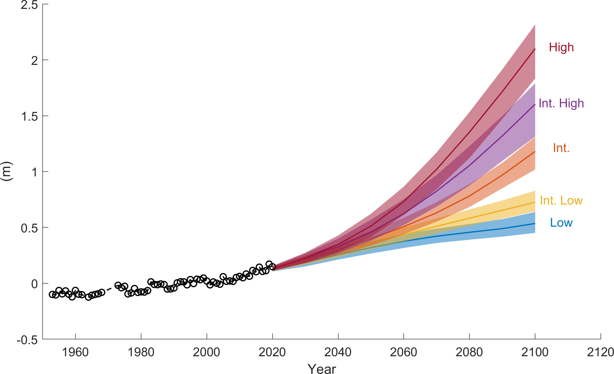
Figure 7 The US southeast SLR projections relative to a baseline of 2000.
The model was run using these three SLR scenarios with model-solution time steps of 2030, 2040, 2050, 2075, and 2100. The long-term historical (1953-2022) SLR trend along the Beaufort coast is 3.4 mm/yr (see Sec 3.3) and thus, each of the three scenarios simulated here represents a significant acceleration of SLR from the historical trend. We note that the long-term trend provides a conservative estimate of sea level change relative to what the site has been experiencing in recent years. Rates of SLR over the past two tidal epochs (1983-2001, and 2002-2020) calculated as the slope of the detrended monthly mean water levels were 2.9 and 8.7 mm/yr, respectively.
3.5 Vegetation and soil data
Field measurements or estimates based on nearby regional studies in NC with sites of similar vegetation types (USFWS studies of national wildlife refuges; http://warrenpinnacle.com/prof/SLAMM/USFWS) provide the majority of non-spatial data used for SLAMM simulations (see Table 3).

Table 3 Main model input parameters.
The elevation of a wetland surface increases as a result of the deposition of inorganic sediments throughout the tidal cycle and the belowground production of biogenic material. Vertical accretion rates depend in part on how often marshes are flooded, and thus are a key factor affecting predictions of future coastal wetland distribution (e.g., Rogers et al., 2013). Based on surface elevation table (SET) data measured at nearby Pivers Island, and at NC Maritime Museum shoreline marshes adjacent to the airport shoreline, the accretion rate for regularly and irregularly flooded marshes was set to 1.5 mm/yr (Currin et al., 2017).
Marsh erosion can be calculated in SLAMM as a function of wave power, which is a function of dominant wind direction, wind speed, fetch, and water depth, but SLAMM assumes erosion occurs over land areas that are in contact with open water and have fetch (i.e., the distance a wave travels across water) larger than 9 km. Maximum fetch around the airport is less than 6 km. Therefore, we estimated the erosion rate by measuring the distance between the historic 1959 and the current shorelines, which is shown in Figure 1B. By averaging the shoreline transition over the 63 yr time period, we calculate an erosion rate of 0.62 m/yr. It is important to note that erosion is not the same across the site and ranges from 0.1 to 1.2 m/yr for 36 transects used over ~1700 m of shoreline (at ~50 m transects spacing).
Lacking site-specific data, values of 1 m/yr and 0.5 m/yr were assigned to swamp and tidal flat erosion, respectively, as these values were commonly used at other SLAMM modeled sites in NC (Table 3). Both values are required model inputs. Swamp erosion in SLAMM can only be projected at the interface between swamps and open water, and since swamps are not exposed to open wave action at this site (see Figure 4) and only cover 0.05% of the total area, this parameter has no significance in this study. It was assumed that beach sedimentation is 0.5 mm/yr, a value commonly used in SLAMM simulations (see other studies in NC; Table 3). Since there is no vegetation to trap suspended sediments on beach shoreface, beach sedimentation rates are generally lower than marsh sedimentation rates.
4 SLAMM conceptual model and calibration
The SLAMM conceptual model makes assumptions about the distribution of the various vegetation cover classes with respect to elevation based on site specific tide range. In general, field-observed relationships between wetland types and elevations are similar to those in SLAMM, however, there are some site-specific differences, particularly in microtidal regimes (Clough et al., 2016). To evaluate the accuracy of the conceptual model for this project site, we used the initial conditions without SLR, accretion, and erosion to compare the conceptual model outputs (e.g., wetland coverage) to the true initial condition (e.g., wetland coverage inputs). This process ensures that the model runs to equilibrium based on current tide ranges and elevation data. Discrepancies between the conceptual model and true starting conditions can result from disagreement between NWI-modeled and true vegetation cover classes and LiDAR uncertainty (particularly in vegetated areas), among other factors. In cases where model predictions do not match the initial wetland types, adjustments can include shifting land elevation, changing tide ranges, and/or altering wetland types as appropriate.
Table 4 provides the minimum allowable elevation for land cover categories and the conversion category that the cells would be reassigned to if their elevation falls below the minimum threshold. Estuarine open water elevation ranges are irrelevant, and this type is merely mentioned to bring the total to 252 ha. We consider the model calibrated when the land cover conversion falls below 5%.
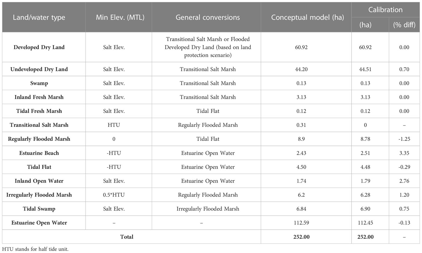
Table 4 Model calibration results and land cover elevations in SLAMM conceptual model and land type conversion when cells fall below their lower elevation range.
The model input analysis (i.e., wetland elevation to tide range relationship) confirms no orderly horizontal offset between the elevation and wetland categories. In addition, conceptual model initial condition results demonstrate that regularly flooded and tidal fresh marsh have large differences (>5%) between the true initial land cover and that predicted by the SLAMM conceptual model, mainly due to the cell elevations that are categorized as tidal flat in the conceptual model.
The conceptual model underpredicted the area of regularly flooded marsh by 33% (i.e., 8.89 ha predicted vs. 13.22 ha observed). As we further analyzed the GIS inundation files (i.e., SLAMM conceptual model output) and the land cover layers (see Table 4), we noticed that this difference is mainly in cells classified in the conceptual model as tidal flats. Therefore, to calibrate the NWI initial input we relabeled regularly flooded marsh areas with elevations below 0-MTL to tidal flat. Tidal fresh marsh is a fresh-water category and therefore must be located above the salt boundary with respect to elevation, otherwise the cells would be converted to tidal flat. A 25% reduction (i.e., from 0.16 to 0.12 ha) has been observed in tidal fresh marsh and following the same approach as described above, we re-categorized that area (0.04 ha) as tidal flat. Analyzing aerial photographs and visiting the site confirm the accuracy of the calibrated land cover layers.
5 Restoration design
As mentioned before (Sec 2), the Michael J. Smith Field airport in NC is a critical regional infrastructure with adjacent shoreline marshes that are highly vulnerable to SLR. The restoration design involves filling and planting ~13.87 ha to restore the marsh shoreline to its historic (1959) extent (see Figure 1B) and installing a series of staggered, overlapping sills at the seaward edge, effectively returning the current erosion rate to 0 m/yr.
The restoration design was informed by on-the-ground analysis of the elevation ranges occupied by existing native plant communities. The restoration design involves placement of dredged sediments to raise the entire footprint to elevations that are appropriate for the target vegetative species (S. alterniflora near the shoreline transitioning to S. patens near the upland boundary). To achieve this transition, we regulate the land elevation in the restoration area with a mild slope from -0.6 and 0.0 m-MTL waterward to 0.8 m-MTL landward (Figure 8). In the model iterations that represent restoration conditions, the input data are recategorized to reflect the restored elevations and starting vegetative communities.
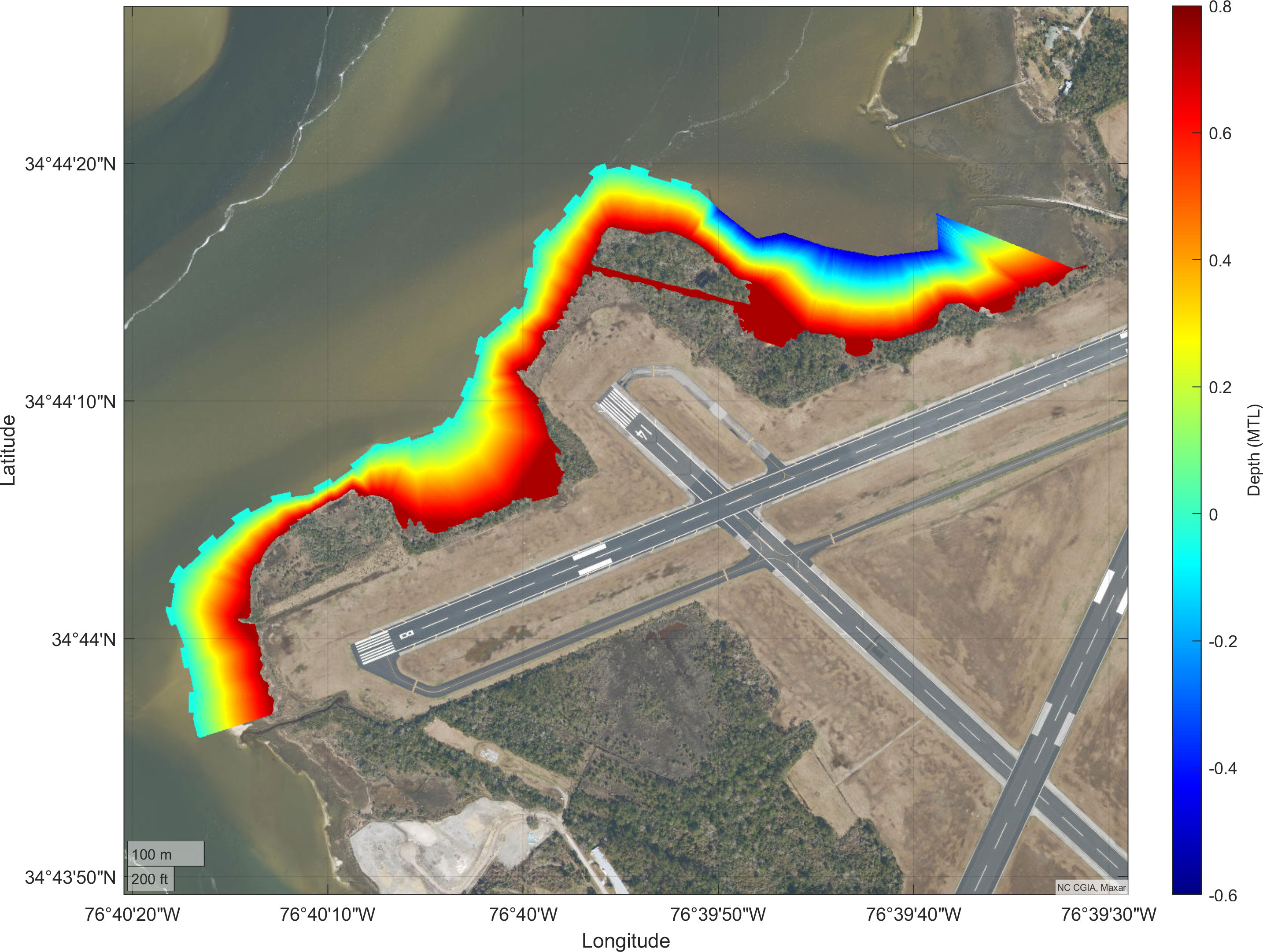
Figure 8 Proposed restoration elevation relative to MTL.
6 Model results
The calibrated model is used with model parameters (see Table 3) and projected SLR to predict the wetland coverage changes under future SLR scenarios for (I) no restoration and (II) restoration conditions.
6.1 No restoration scenario
Modeling three SLR scenarios with no site modification (i.e., no restoration) reveals a consistent pattern of salt marsh expanding into fresh marsh, salt marsh transitioning to higher elevations, and substantially larger flooded marshes and open water areas at relatively high rates of SLR. Model results suggest that several land-cover categories are vulnerable to accelerated SLR scenarios. In particular, current irregularly flooded marshes (higher elevation marshes) are predicted to lose 1.41-3.62 ha (~23-60%) of their current area by 2100 under intermediate and high SLR scenarios, respectively (Figures 9, 10). However, some of the losses of the irregularly flooded marshes will be compensated by the creation of new salt marshes through upland migration as dry lands are predicted to convert to transitional salt marsh when regularly inundated (see Figure 9). By 2100, much of the area initially categorized as regularly flooded marsh is converted to estuarine beach and tidal flat under all SLR scenarios.
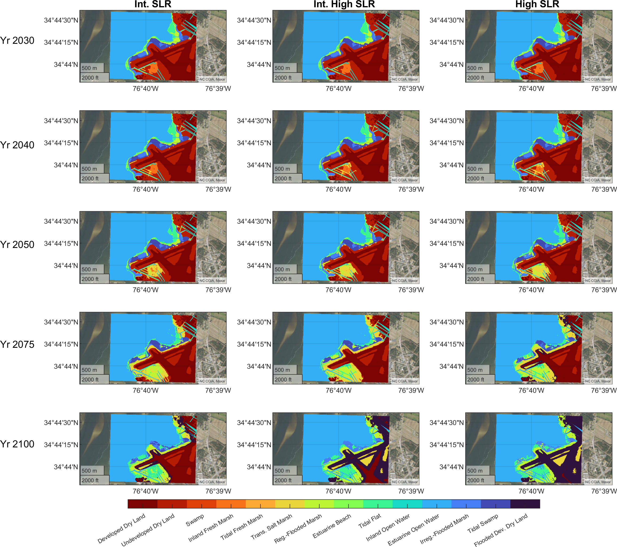
Figure 9 Projected coverage area changes over time for each three different SLR scenarios by 2100 with no restoration.
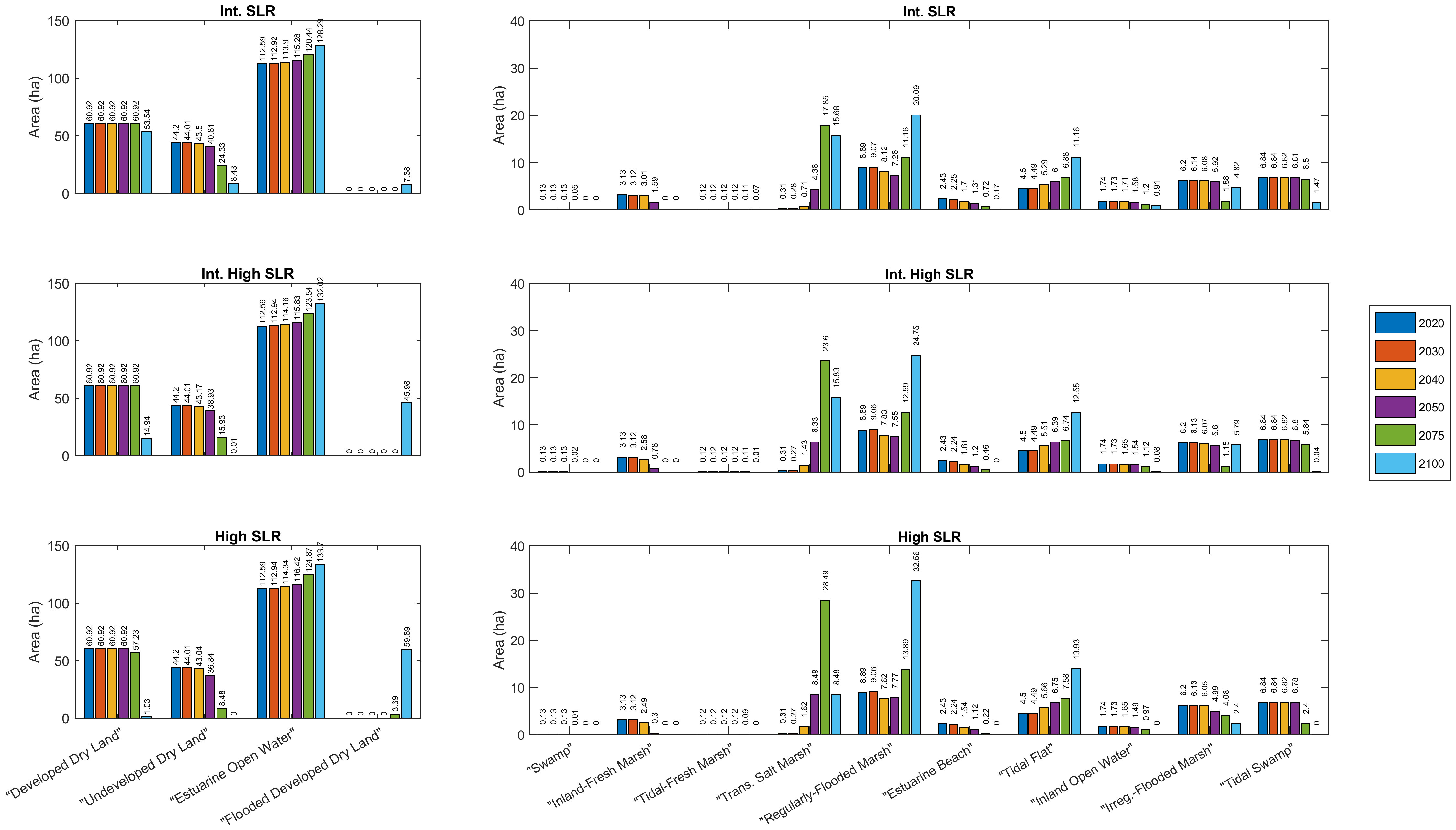
Figure 10 Land coverage changes over time for three different SLR scenarios with no restoration. For each category, the bars represent the area for that land/water cover type for each model year (i.e., 2020, 2030, 2040, 2050, 2075, 2100). Note that subplot panels have different vertical axis limits.
On the other hand, regularly flooded (low elevation marshes) are predicted to gain ~127% to 270% of their current coverage by 2100. Overall, tidal marsh areas (regularly flooded, irregularly flooded, transitional, and tidal-fresh marshes) are predicted to increase by ~20.23 ha by 2100, which means that the overall losses reduce with higher SLR scenarios by 2100. Significant reductions in tidal swamp, tidal fresh marsh, and estuarine beaches are also expected with increasing SLR by 2100 (Figures 9, 10). Simulations conducted using higher SLR scenarios suggest that inland fresh marshes will be unable to adjust to higher SLR rates because higher water levels will penetrate farther inland and eliminate them. The comparison of wetland resilience between intermediate and high SLR simulations shows a similarity to SLAMM modeling of lagoon marshes in Portugal (Carrasco et al., 2021), in which nonlinearity in wetland responses to SLR are reported.
In Table 5 we sum the areas from individual wetland categories (Figure 10) to create broader categories for simpler comparisons between wetland changes. Table 5 describes which wetland types were combined to create these broader categories.
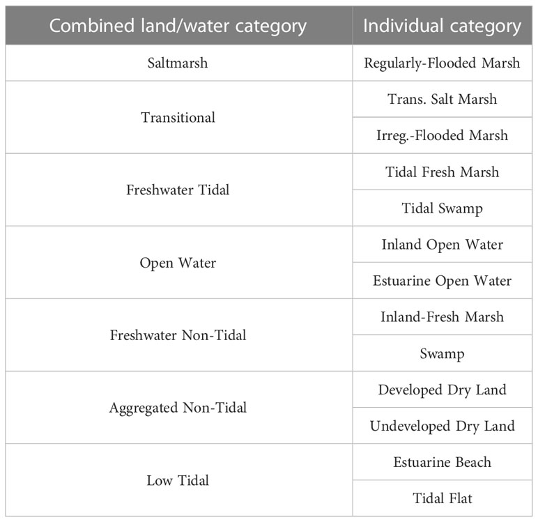
Table 5 Land/water types merged to form combined categories.
Aggregated non-tidal (i.e., combined developed and undeveloped dry land) area continues to decrease at a relatively low rate until 2050 under all SLR scenarios. The magnitude of losses in these areas increases in years 2075 and 2100. Most of the changes are due to conversion of dry land to low tidal and open water areas (Table 6).
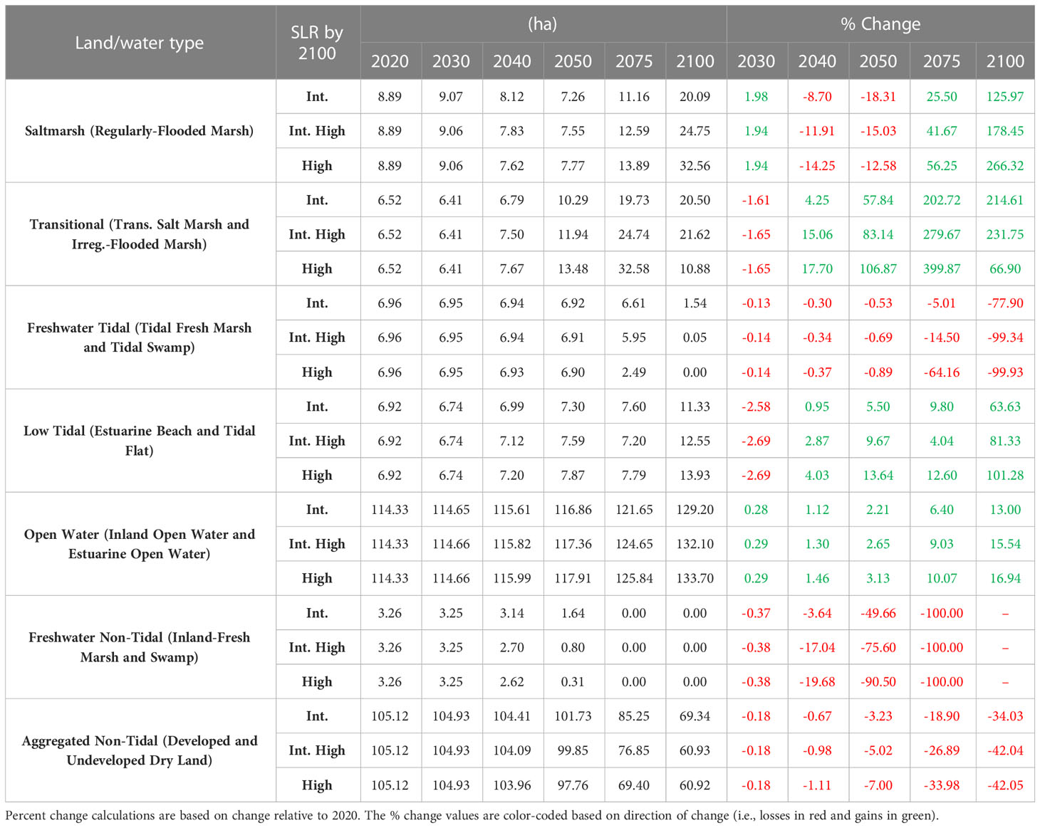
Table 6 Projected changes in land/water categories from initial time (2020) to 2100 for three SLR scenarios with no restoration (Int. SLR=1.12m, Int. High SLR=1.54m, High SLR=2.04m).
The salt marsh area would initially increase 2% by 2030 and then drop by 8.7% to 18.3% by 2040 and 2050, and then increase again as transitional and parts of undeveloped dry lands would be converted to salt marshes (see Table 6 and Figure 9). The largest changes in the transitional category (combined trans. salt and irreg.-flooded marsh) will occur from mid- to late-century and represent the largest gains of any of the wetland types. Under all three projected SLR scenarios and in all model years, freshwater tidal marsh losses are caused by rising water levels and surrounding elevations (see also Figure 2), while the non-tidal freshwater would disappear by 2075.
6.2 Restoration scenario
Projected SLR-induced changes in land/water categories are shown in Figure 11, illustrating the potential alterations in the distribution of these categories in the future. Table 7 shows numerical results for projected wetlands and percentage of difference between no-restoration and restoration conditions. Low tidal areas and salt marshes experience the most significant change (i.e., positive % change in Table 7) by gaining area under the restoration condition. Model results show that the restoration scenario is more effective in maintaining the salt marsh habitat than the no restoration scenario under all three SLR projections. Specifically, the restoration scenario is associated with an average decrease of ~2.8% in open water and an average increase of ~75% in salt marsh habitat compared to the no-restoration scenario until the year 2050 (Table 7).

Figure 11 Projected spatial distribution of land cover over time for each three different SLR scenarios by 2100 with restoration.
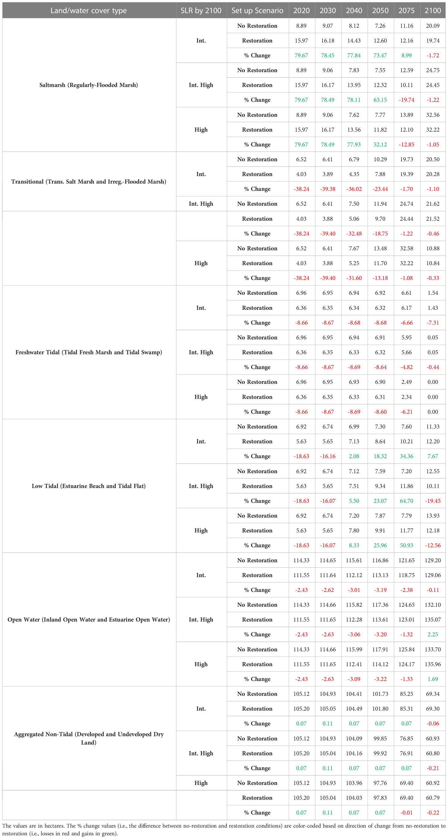
Table 7 Projected changes in land/water categories between the restoration and no-restoration conditions for three SLR scenarios (Int. SLR=1.12m, Int. High SLR=1.54m, High SLR=2.04m).
The restoration project would result in increased cover of regularly flooded salt marsh through mid-century. The restoration configuration will differ from the no-restoration less over time as projected SLR increases, and all existing shoreline marsh will be submerged and classified as open water by the end of the century (2100) under both conditions.
In general, the wetland categories show similar trends across all three SLR scenarios. Low tidal areas experience net gains under intermediate, intermediate-high, and high SLR scenarios in 2040, 2050, 2075 and a small gain under intermediate SLR in 2075, then a net loss in area under intermediate-high and high SLR after 2075.
Overall, transitional (i.e., irregularly flooded) area is vulnerable habitat under restoration condition and projected SLR with an average projected decline of ~22%. The modeled predictions under three SLR scenarios with restoration condition suggest that salt marsh would be resilient to SLR by 2075 before being inundated and converted to tidal flat and later to open water.
7 Discussion and conclusion
Increasing SLR trends pose a threat to much of our coastal infrastructure and the natural systems that protect it (IPCC, 2012; Sweet et al., 2022). Coastal cities and communities around the world are at risk of inundation, storm surges, and flooding, which can cause severe damage to homes, businesses, and critical infrastructure such as ports, airports, and power plants. Moreover, many of the natural systems that protect these coastal areas, such as wetlands, are also under threat from SLR and erosion. For example, in the coming decades, the global extent of coastal salt marsh is predicted to decrease dramatically due to the inability of these systems to keep pace with accelerating SLR (Horton et al., 2018; Osland et al., 2022). Losses in salt marsh habitat are also projected along the mid-Atlantic and gulf coasts (Waldron et al., 2021; Warnell et al., 2022). The coastal regions of NC have experienced substantial land-cover changes over the past 50 years due to suburban development, silviculture, and agriculture, as well as shoreline erosion (Bost et al., 2023). These changes, combined with the region’s relatively low tide range (<1m) and suspended sediment supply, have made the marshes in NC particularly susceptible to SLR (Kirwan et al., 2010; Warnell et al., 2022). As a result, there is an urgent need to implement strategies that can enhance the resilience of coastal infrastructure and protect the natural systems that support it in the face of SLR and other climate-related stressors.
Here, we investigate how the use of dredged sediments to restore coastal fringing wetlands to their historical extent can be used to sustain these critical habitats against rising sea levels. The particular study site’s coastal wetlands protect critical infrastructure in NC and have experienced significant shoreline erosion in recent decades. The developed model was parameterized with site-specific data and applied to predict effects of future SLR on wetland types and migration given SLR scenarios ranging from 1.12 m to 2.04 m by 2100. Model results suggest overall delayed losses of salt marsh under the restoration condition, which means that under all SLR scenarios, the restoration condition creates and maintains more salt marsh habitat than no-restoration condition for a longer period of time. The proportion of wetland changes (Tables 6, 7) is sensitive to the rate of SLR, and the proposed restoration project (i.e., application of dredged sediment) would result in increased salt marsh coverage through mid-century. Afterward, the restoration configuration will not have a significant impact compared to the no-restoration configuration as the projected SLR increases because, regardless of starting condition, existing shoreline marshes will be submerged and converted to open water by the end of the century (2100). Restoration would result in an increase of ~50-80% of salt marsh area by 2030-2050 under all SLR projections. Much of this increase in marsh over time is at the expense of upland, while the restoration scenario provides protection against erosion, it does not stop the marsh from migrating closer to the runway or mitigate the susceptibility of the adjacent uplands to SLR. Under both the intermediate-high and high SLR scenarios, the runways are flooded by 2100 regardless of project implementation.
It is important to note that SLAMM assumes a linear relationship between SLR and marsh migration, meaning that the rate of marsh migration will be constant over time. However, in reality, the rate of migration may be affected by factors such as sediment availability, elevation gain, and the presence of barriers, which could lead to non-linear patterns of marsh migration and impact the accuracy of our model’s predictions. Additionally, we assumed no changes in land use or development patterns that could impact the availability of suitable habitat for marsh migration uplands.
In conclusion, this study provides insight into the efficacy of NBS for mitigating the future impacts of SLR in coastal regions. Understanding SLR and marsh interactions in coastal wetlands has important implications for system management and flood protection. By working with natural systems, NBS can help to enhance resilience and reduce the vulnerability of critical infrastructure to climate change and other environmental stressors. Additionally, these solutions extend the provision of marsh co-benefits such as carbon sequestration, biodiversity conservation, water quality improvement, fishery habitat, and recreational opportunities. Therefore, investing in NBS can be a win-win approach for protecting critical infrastructure while also promoting ecological sustainability. The results presented here can help decision makers and engineers better understand the effects of SLR and restoration on marsh resilience, and therefore help provide a better environment for marsh survival.
Data availability statement
The original contributions presented in the study are included in the article/supplementary material. Further inquiries can be directed to the corresponding author.
Author contributions
RF: Conceptualization, Methodology, Modeling, Visualization, Writing, Review and Editing. JD: Conceptualization, Formal Analysis, Writing, Review and Editing. CC: Conceptualization, Review and Editing. MH: Design, Review and Editing. SC: Review and Editing. All authors contributed to the article and approved the submitted version.
Funding
This work was supported and funded by the NOAA, Effects of Sea Level Rise Program (ESLR), Grant number NA20NOS4780192.
Acknowledgments
We thank Brandon Puckett, Molly Bost, Tomma Barnes, and the reviewers for their thoughtful feedback on the manuscript.
Conflict of interest
Author RF was employed by Consolidated Safety Services, Inc. Authors MH and CC were employed by the company EA Engineering Group.
The remaining authors declare that the research was conducted in the absence of any commercial or financial relationships that could be construed as a potential conflict of interest.
Publisher’s note
All claims expressed in this article are solely those of the authors and do not necessarily represent those of their affiliated organizations, or those of the publisher, the editors and the reviewers. Any product that may be evaluated in this article, or claim that may be made by its manufacturer, is not guaranteed or endorsed by the publisher.
References
Alizad K., Medeiros S. C., Foster-Martinez M. R., Hagen S. C. (2020). Model sensitivity to topographic uncertainty in meso- and microtidal marshes. IEEE J. Selected Topics Appl. Earth Observ. Remote Sens. 13, 807–814. doi: 10.1109/JSTARS.2020.2973490
Arkema K. K., Guannel G., Verutes G., Wood S. A., Guerry A., Ruckelshaus M., et al. (2013). Coastal habitats shield people and property from sea-level rise and storms. Nat. Climate Change 3, 913–918. doi: 10.1038/nclimate1944
Bendoni M., Mel R., Solari L., Lanzoni S., Francalanci S., Oumeraci H. (2016). Insights into lateral marsh retreat mechanism through localized field measurements. Water Resour. Res. 52, 1446–1464. doi: 10.1002/2015WR017966
Bilkovic D. M., Roggero M., Hershner C. H., Havens K. H. (2006). Influence of land use on macrobenthic communities in nearshore estuarine habitats. Estuaries Coasts 29, 1185–1195. doi: 10.1007/BF02781819
Bost M. C., Deaton C. D., Rodriguez A. B., McKee B. A., Fodrie F. J., Miller C. B. (2023). Anthropogenic impacts on tidal creek sedimentation since 1900. PLoS One 18, e0280490. doi: 10.1371/journal.pone.0280490
Bozek C. M., Burdick D. M. (2005). Impacts of seawalls on saltmarsh plant communities in the great bay estuary, new Hampshire USA. Wetlands Ecol. Manage. 13, 553–568. doi: 10.1007/s11273-004-5543-z
Campbell A. D., Fatoyinbo L., Goldberg L., Lagomasino D. (2022). Global hotspots of salt marsh change and carbon emissions. Nature 612, 701–706. doi: 10.1038/s41586-022-05355-z
Carrasco A. R., Kombiadou K., Amado M., Matias A. (2021). Past and future marsh adaptation: lessons learned from the ria Formosa lagoon. Sci. Total Environ. 790, 148082. doi: 10.1016/j.scitotenv.2021.148082
Clough J., Polaczyk A., Propato M. (2016). Modeling the potential effects of sea-level rise on the coast of new York: integrating mechanistic accretion and stochastic uncertainty. Environ. Model. Software 84, 349–362. doi: 10.1016/j.envsoft.2016.06.023
Costanza R., de Groot R., Sutton P., van der Ploeg S., Anderson S. J., Kubiszewski I., et al. (2014). Changes in the global value of ecosystem services. global environmental change Glob. Environ. Change 26, 152–158. doi: 10.1016/j.gloenvcha.2014.04.002
Costanza R., Pérez-Maqueo O., Martinez M. L., Sutton P., Anderson S. J., Mulder K. (2008). The value of coastal wetlands for hurricane protection. AMBIO: A J. Hum. Environ. 37, 241–248. doi: 10.1579/0044-7447(2008)37[241:tvocwf]2.0.co;2
Craft C., Clough J., Ehman J., Joye S., Park R., Pennings S., et al. (2009). Forecasting the effects of accelerated sea-level rise on tidal marsh ecosystem services. Front. Ecol. Environ. 7, 73–78. doi: 10.1890/070219
Crosby S. C., Sax D. F., Palmer M. E., Booth H. S., Deegan L. A., Bertness M. D., et al. (2016). Salt marsh persistence is threatened by predicted sea-level rise. Estuarine Coast. Shelf Sci. 181, 93–99. doi: 10.1016/j.ecss.2016.08.018
Currin C. A., Davis J., Malhotra A., Currin C. A. (2017). Response of salt marshes to wave energy provides guidance for successful living shoreline implementation. In Bilkovic J., Toft M., Mitchell M., La Peyre M. (eds), (Living Shorelines: The Science and Management of Nature-based Coastal Protection, CRC Press, Taylor & Francis Group). pp. 211–234.
Currin C. A. (2019). “Chapter 30 - living shorelines for coastal resilience,” in Coastal wetlands, 2nd ed. Eds. Perillo G. M. E., Wolanski E., Cahoon D. R., Hopkinson C. S. (Elsevier), 1023–1053. Available at: https://www.sciencedirect.com/science/article/pii/B9780444638939000307.
Dahl T. E. (2011). Status and trends of wetlands in the conterminous united states 2004 to 2009 (Washington, D. C: U.S. Department of the Interior; Fish and Wildlife Service), 108.
Duarte C. M., Losada I. J., Hendriks I. E., Mazarrasa I., Marbà N. (2013). The role of coastal plant communities for climate change mitigation and adaptation. Nat. Climate Change 3, 961–968. doi: 10.1038/nclimate1970
Dugan J. E., Airoldi L., Chapman M. G., Walker S. J., Schlacher T. (2011). “8.02 - estuarine and coastal structures: environmental effects, a focus on shore and nearshore structures,” in Treatise on estuarine and coastal science. Eds. Wolanski E., McLusky D. (Waltham: Academic Press), 17–41.
Gilby B. L., Weinstein M. P., Baker R., Cebrian J., Alford S. B., Chelsky A., et al. (2021). Human actions alter tidal marsh seascapes and the provision of ecosystem services. Estuaries Coasts 44, 1628–1636. doi: 10.1007/s12237-020-00830-0
Gittman R. K., Fodrie F. J., Popowich A. M., Keller D. A., Bruno J. F., Currin C. A., et al. (2015). Engineering away our natural defenses: an analysis of shoreline hardening in the US. Front. Ecol. Environ. 13, 301–307. doi: 10.1890/150065
Gittman R. K., Scyphers S. B., Smith C. S., Neylan I. P., Grabowski J. H. (2016). Ecological consequences of shoreline hardening: a meta-analysis. BioScience 66, 763–773. doi: 10.1093/biosci/biw091
Glick P., Clough J., Polaczyk A., Couvillion B., Nunley B. (2013). Potential effects of Sea-level rise on coastal wetlands in southeastern Louisiana. J. Coast. Res. 63, 211–233. doi: 10.2112/SI63-0017.1
Horton B. P., Shennan I., Bradley S. L., Cahill N., Kirwan M., Kopp R. E., et al. (2018). Predicting marsh vulnerability to sea-level rise using Holocene relative sea-level data. Nat. Commun. 9, 2687. doi: 10.1038/s41467-018-05080-0
IPCC (2007). Climate change 2007: synthesis report. contribution of working groups I, II and III to the fourth assessment report of the intergovernmental panel on climate change. Eds. Pachauri R. K., Reisinger A. (Geneva, Switzerland: IPCC). Core Writing Team.
IPCC (2012). Managing the risks of extreme events and disasters to advance climate change adaptation. a special report of working groups I and II of the intergovernmental panel on climate change. Eds. Field C. B., Barros V., Stocker T. F., Qin D., Dokken D. J., Ebi K. L., Mastrandrea M. D., Mach K. J., Plattner G.-K., Allen S. K., Tignor M., Midgley P. M. (Cambridge, UK, and New York, NY, USA: Cambridge University Press), 582.
Karl T. R., Melillo J. M., Peterson T. C. (2009). Global climate change impacts in the united states (New York, NY: Cambridge University Press).
Kirwan M. L., Guntenspergen G. R. (2012). Feedbacks between inundation, root production, and shoot growth in a rapidly submerging brackish marsh. J. Ecol. 100, 764–770. doi: 10.1111/j.1365-2745.2012.01957.x
Kirwan M. L., Guntenspergen G. R., D'Alpaos A., Morris J. T., Mudd S. M., Temmerman S. (2010). Limits on the adaptability of coastal marshes to rising sea level. Geophysical Res. Lett. 37. doi: 10.1029/2010GL045489
Kirwan M. L., Murray A. B. (2008). Ecological and morphological response of brackish tidal marshland to the next century of sea level rise: westham island, British Columbia. Global Planetary Change 60, 471–486. doi: 10.1016/j.gloplacha.2007.05.005
Mogensen L. A., Rogers K. (2018). Validation and comparison of a model of the effect of Sea-level rise on coastal wetlands. Sci. Rep. 8, 1369. doi: 10.1038/s41598-018-19695-2
Möller I. (2019). Applying uncertain science to nature-based coastal protection: lessons from shallow wetland-dominated shores. Front. Environ. Sci. 7. doi: 10.3389/fenvs.2019.00049
Möller I., Kudella M., Rupprecht F., Spencer T., Paul M., van Wesenbeeck B. K., et al. (2014). Wave attenuation over coastal salt marshes under storm surge conditions. Nat. Geosci. 7, 727–731. doi: 10.1038/ngeo2251
Narayan S., Beck M. W., Wilson P., Thomas C. J., Guerrero A., Shepard C. C., et al. (2017). The value of coastal wetlands for flood damage reduction in the northeastern USA. Sci. Rep. 7, 9463. doi: 10.1038/s41598-017-09269-z
Nicholls R. J., Hanson S. E., Lowe J. A., Warrick R. A., Lu X., Long A. J. (2014). Sea-Level scenarios for evaluating coastal impacts. WIREs Climate Change 5, 129–150. doi: 10.1002/wcc.253
Nicholls R. J., Wong P. P., Burkett V. R., Codignotto J. O., Hay J. E., McLean R. F., et al. (2007). “Coastal systems and low-lying areas,” in Climate change 2007: impacts, adaptation and vulnerability. contribution of working group II to the fourth assessment report of the intergovernmental panel on climate change. M.L. Parry, O.F.
Osland M. J., Chivoiu B., Enwright N. M., Thorne K. M., Guntenspergen G. R., Grace J. B., et al. (2022). Migration and transformation of coastal wetlands in response to rising seas. Sci. Adv. 8, eabo5174. doi: 10.1126/sciadv.abo5174
Polk M. A., Gittman R. K., Smith C. S., Eulie D. O. (2022). Coastal resilience surges as living shorelines reduce lateral erosion of salt marshes. Integ. Environ. Assess. Manage. 18, 82–98. doi: 10.1002/ieam.4447
Rogers K., Saintilan N., Copeland C. (2013). Reprint of modelling wetland surface elevation dynamics and its application to forecasting the effects of sea-level rise on estuarine wetlands. Ecol. Model. 264, 27–36. doi: 10.1016/j.ecolmodel.2013.04.016
Smith C. S., Rudd M. E., Gittman R. K., Melvin E. C., Patterson V. S., Renzi J. J., et al. (2020). Coming to terms with living shorelines: a scoping review of novel restoration strategies for shoreline protection. Front. Mar. Sci. 7. doi: 10.3389/fmars.2020.00434
Spencer T., Schuerch M., Nicholls R. J., Hinkel J., Lincke D., Vafeidis A. T., et al. (2016). Global coastal wetland change under sea-level rise and related stresses: the DIVA wetland change model. Global Planetary Change 139, 15–30. doi: 10.1016/j.gloplacha.2015.12.018
Sweet W. V., Hamlington B. D., Kopp R. E., Weaver C. P., Barnard P. L., Bekaert D., et al. (2022). Global and regional Sea level rise scenarios for the united states: updated mean projections and extreme water level probabilities along U.S. coastlines. NOAA technical report NOS 01 (Silver Spring, MD: National Oceanic and Atmospheric Administration, National Ocean Service), 111.
Temmerman S., Meire P., Bouma T. J., Herman P. M. J., Ysebaert T., De Vriend H. J. (2013). Ecosystem-based coastal defence in the face of global change. Nature 504, 79–83. doi: 10.1038/nature12859
Valle-Levinson A., Dutton A., Martin J. B. (2017). Spatial and temporal variability of sea level rise hot spots over the eastern united states. Geophysical Res. Lett. 44, 7876–7882. doi: 10.1002/2017GL073926
Waldron M. C. B., Carter G. A., Biber P. D. (2021). Using aerial imagery to determine the effects of sea-level rise on fluvial marshes at the mouth of the pascagoula river (Mississippi, USA). J. Coast. Res. 37 (2), 389–407. doi: 10.2112/JCOASTRES-D-20-00037.1
Keywords: coastal resilience, nature-based solutions, sea-level rise, SLAMM, restoration
Citation: Familkhalili R, Davis J, Currin CA, Heppe ME and Cohen S (2023) Quantifying the benefits of wetland restoration under projected sea level rise. Front. Mar. Sci. 10:1187276. doi: 10.3389/fmars.2023.1187276
Received: 15 March 2023; Accepted: 19 May 2023;
Published: 06 June 2023.
Edited by:
Jamie Ruprecht, University of New South Wales, AustraliaReviewed by:
Maike Paul, Leibniz University Hannover, GermanyPatrick Biber, University of Southern Mississippi, United States
Copyright © 2023 Familkhalili, Davis, Currin, Heppe and Cohen. This is an open-access article distributed under the terms of the Creative Commons Attribution License (CC BY). The use, distribution or reproduction in other forums is permitted, provided the original author(s) and the copyright owner(s) are credited and that the original publication in this journal is cited, in accordance with accepted academic practice. No use, distribution or reproduction is permitted which does not comply with these terms.
*Correspondence: Ramin Familkhalili, cmFtaW4uZmFtaWxraGFsaWxpQG5vYWEuZ292