Toward efficient deep learning system for in-situ plankton image recognition

Plankton is critical for the structure and function of marine ecosystems. In the past three decades, various underwater imaging systems have been developed to collect in-situ plankton images and image processing has been a major bottleneck that hinders the deployment of plankton imaging systems. In recent years, deep learning methods have greatly enhanced our ability of processing in-situ plankton images, but high-computational demands and longtime consumption still remain problematic. In this study, we used knowledge distillation as a framework for model compression and improved computing efficiency while maintaining original high accuracy. A novel inter-class similarity distillation algorithm based on feature prototypes was proposed and enabled the student network (small scale) to acquire excellent ability for plankton recognition after being guided by the teacher network (large scale). To identify the suitable teacher network, we compared emerging Transformer neural networks and convolution neural networks (CNNs), and the best performing deep learning model, Swin-B, was selected. Utilizing the proposed knowledge distillation algorithm, the feature extraction ability of Swin-B was transferred to five more lightweight networks, and the results had been evaluated in taxonomic dataset of in-situ plankton images. Subsequently, the chosen lightweight model and the Bilateral–Sobel edge enhancement were tested to process in-situ images with high level of noises captured from coastal waters of Guangdong, China and achieved an overall recall rate of 91.73%. Our work contributes to effective deep learning models and facilitates the deployment of underwater plankton imaging systems by promoting both accuracy and speed in recognition of plankton targets.

1 Introduction

Plankton play a pivotal role in marine food webs and are essential for integrated ecosystem assessment (Brun et al., 2015; Piredda et al., 2017; Braz et al., 2020). For example, plankton often provide information on living resources (Wang et al., 2022), environmental conditions (Lv et al., 2022), and fisheries (Azani et al., 2021). Effective monitoring of plankton allows researchers to deduce their dynamics and identify the underlying processes (Bi et al., 2022). Thus underwater imaging systems are increasingly being deployed to collect in-situ plankton images on various platforms (Davis et al., 1996; Benfield et al., 2000; Gorsky et al., 2000; Cowen and Guigand, 2008) to estimate abundances of different plankton groups and examine their spatial and temporal dynamics (Bi et al., 2013; Hermand et al., 2013; Guo et al., 2018; Luo et al., 2018). In recent years, imaging systems have increasingly been used for high-frequency long-term plankton monitoring (Campbell et al., 2020; Orenstein et al., 2020; Song et al., 2020; Bi et al., 2022).

In plankton image processing, it is difficult to balance accuracy and processing speed. To improve accuracy, researchers utilize not only advanced optical mechanisms to acquire more information (Buskey and Hyatt, 2006; Hermand et al., 2013; Guo et al., 2018) but also deep learning systems to achieve high accuracy (Li and Cui, 2016; Luo et al., 2018; Kyathanahally et al., 2021; Li et al., 2021; Kyathanahally et al., 2022). As a result of these evolutions, the speeds of computing have dropped, making it difficult to deploy excellent algorithms on site because of the following: (1) The amount of raw data increases with the continuous sampling; (2) neural networks in deep learning have a huge number of parameters and computations; (3) as data transmission is often limited in open ocean, the processing ability of underwater computing hardware is extremely limited. Therefore, it is necessary to develop portable data processing procedures for independent underwater equipment to deal with abovementioned problems. In other words, the algorithm should be improved in terms of computing speed and storage capacity while ensuring the accuracy and generalization.

In the era of deep learning, researchers try to compress the neural network models to reduce the amount of parameters and complexity of calculation. The mainstream methods include model pruning (Tanaka et al., 2020), model quantization (Fan et al., 2020), parameter sharing (Wu et al., 2018), and knowledge distillation (Hinton et al., 2015). Knowledge distillation is able to realize the interaction of parameters and features among multiple neural networks and possesses excellent performance and flexibility. In general, large-scale models tend to have better learning abilities and can accurately extract the key features of the samples in datasets. According to the core idea of knowledge distillation, large-scale models are taken as the teacher networks, and the iterative operations aim to reduce the loss function between the probability distributions or feature vectors output of the teacher networks and other smaller scale models (called the student networks). With the progress of training, the student networks gradually learn the feature extraction mechanisms guided by the teacher networks. It means that small-scale models can achieve equal accuracy in specific tasks as large-scale models through this method. Knowledge distillation was proposed by Hinton et al., 2015 and initially used Kullback–Leibler (KL) divergence as the loss function. Subsequently, various works were proposed in multiple distillation strategies. For example, Romero et al., 2014 proposed the distillation method using feature maps computed by middle layers in neural network (FitNet). Peng et al., 2019 and Tung and Mori, 2019 demonstrated the distillation processes based on correlation congruence (CC) and similarity preserving (SP), respectively. Similarly, it is also worth exploring to propose model compressing techniques in the scenarios of in-situ plankton image processing.

Based on the characters of PlanktonScope (an in-situ underwater imaging system proposed by Bi et al., 2022 and attached algorithm pipeline), the present study attempts to introduce knowledge distillation method and demonstrate efficient detection and recognition tasks on in-situ plankton images. We designed and implemented an inter-class similarity distillation algorithm based on feature prototype projection (prototype projection distillation, PPD) to realize the compression of forward calculation model. In order to seek the appropriate teacher network and ensure the original accuracy, we carried out a comparative study and examined the accuracy of five convolution neural networks (CNNs) and three Transformer architectures. Combined with transfer learning, the Swin-B network model (from Transformer architectures) was found to express the highest accuracy and was selected as the preliminary algorithm for classification (teacher network). Meanwhile, a Bilateral–Sobel edge enhancement method was proposed to highlight the edge pixel regions of targets to suppress the noise and background of in-situ images. This technique aimed to solve the segmentation difficulties caused by noise stickiness and edge destruction. Finally, the selected student networks and Bilateral–Sobel edge enhancement were integrated into algorithm pipeline, and these schemes were evaluated in accuracy and time consumption on the dataset captured via PlanktonScope in the coastal areas of Guangdong, China.

2 Materials and methods

The knowledge distillation and edge enhancement method are employed in the procedures of recognition and detection in algorithm pipeline, respectively. In Section 2.1, the algorithm pipeline of PlanktonScope is presented and the datasets applied in experiments are described. In Section 2.2, the basic theory and mathematical model of the proposed inter-class similarity knowledge distillation method based on feature prototype projection (PPD) are illustrated in details. In Section 2.3, as candidates for the teacher network in distillation, Transformer and CNN model families are described. In Section 2.4, the Bilateral–Sobel edge enhancement algorithm used to improve effect of detection is presented.

2.1 Description of algorithm pipeline and datasets

2.1.1 Basic algorithm pipeline of PlanktonScope

Figure 1 presents the content of algorithm pipeline. Plankton image detection and recognition include two stages: extraction and classification (Bi et al., 2015). Extraction is to extract the pixel regions of the targets from the in-situ images to separate the targets and background. Classification is to extract the features of the segmented targets and judge the class of the targets according to their features. The steps can be summarized as follows: (1) input the in-situ image and adjust the brightness; (2) operate denoising and edge enhancement; (3) implement the threshold segmentation proposed by (Otsu, 1979) based on maximum between-cluster variance to finish binarization; (4) demonstrate the morphological closing operation (Said et al., 2016) to fill the discontinuities, holes, and edge breaks; (5) implement the contour extraction based on boundary tracking (Suzuki, 1985; Marini et al., 2018) to obtain the regions of interest (ROIs) of the targets; (6) classify the detected targets using the selected calculation model; and (7) operate statistics of the quantity and species of plankton. The contributions of PPD method and Bilateral–Sobel edge enhancement are in steps (6) and (2), respectively.

FIGURE 1

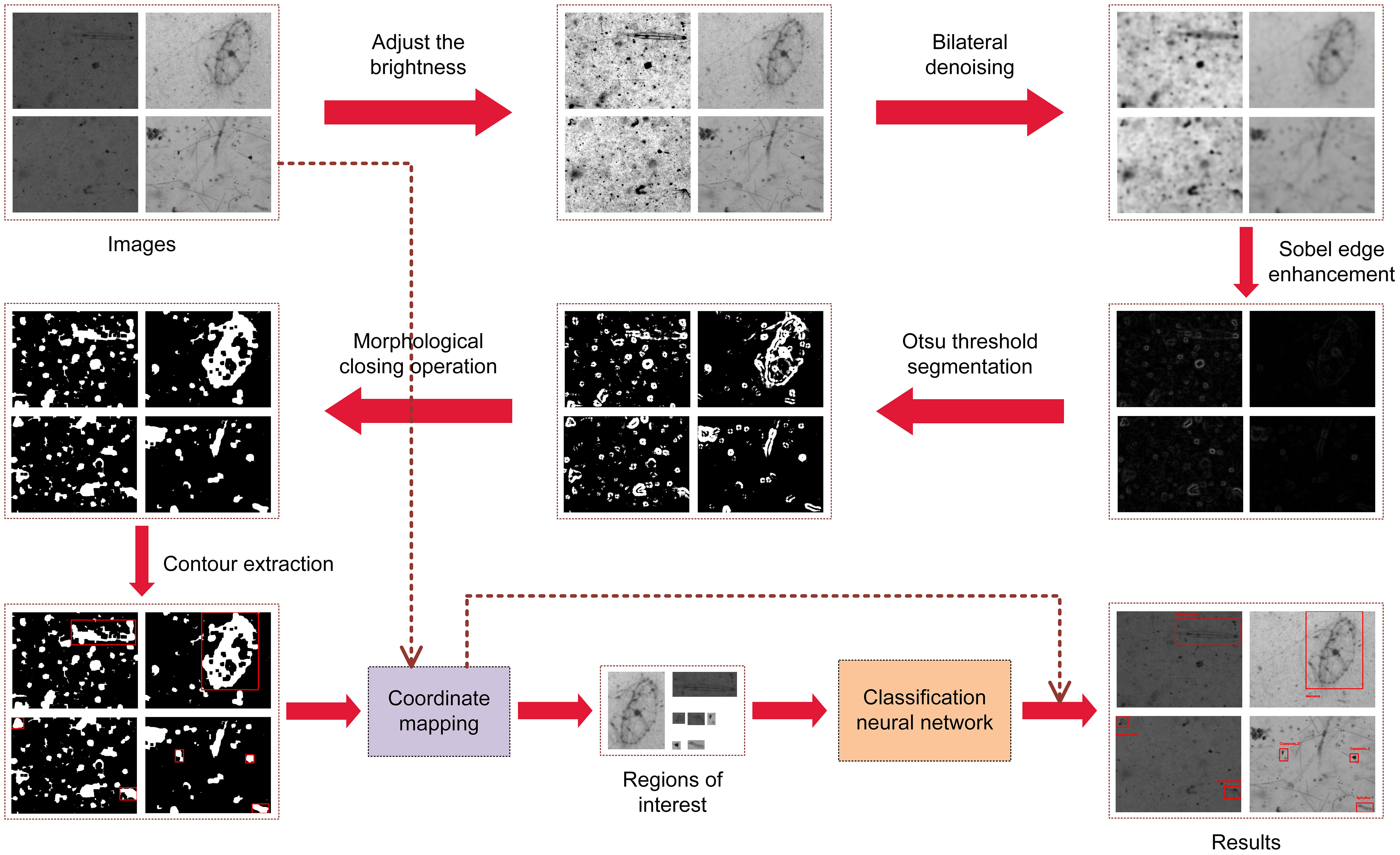
Figure 1 The flowchart of the algorithm pipeline and related results.

2.1.2 Test dataset for detection and recognition tasks

The dataset for efficiency test of the proposed methods was collected by PlanktonScope in the coastal area of Guangdong, China. This dataset contains 209 in-situ images (2180 × 1635) for testing. These images are all 8-bit, and the whole set contains a total of 494 plankton targets, of which 258 are Medusaes. In addition, the other classes include Copepoda, Spirulina, Appendicularia, Chaetognatha, and Echinodermata (in Figure 2). The ground truths of ROIs are manually annotated. As the result of deep diving depth and illumination conditions of the monitoring system, the collected in-situ images are relatively dark, with pixel value of brightness ranging from 22 to 163. Even the human eye cannot distinguish a target in such weak contrast. Therefore, brightness adaptive processing is carried out for images:

FIGURE 2

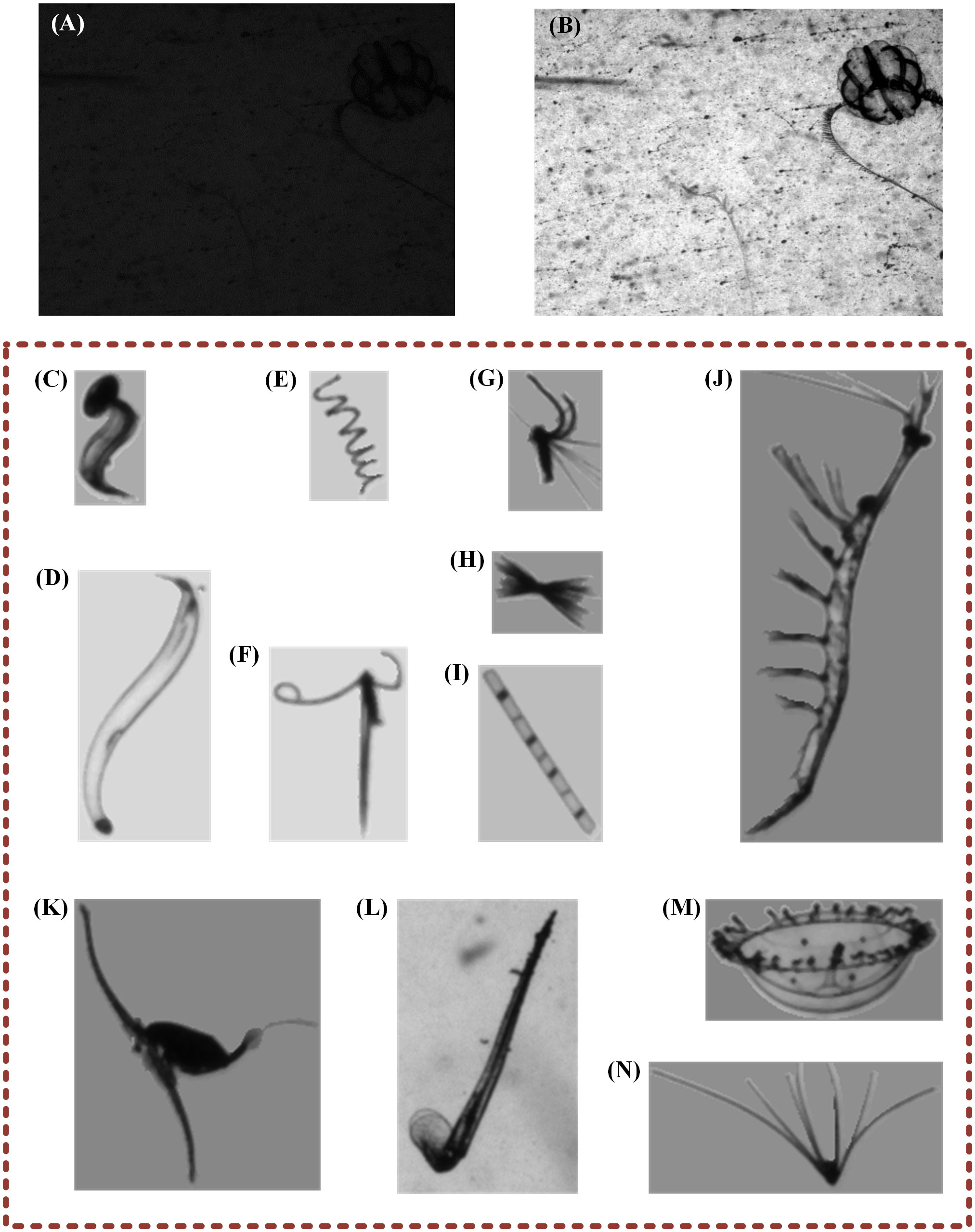
Figure 2 Samples of datasets. (A) Original image before brightness adjustment; (B) processed result after brightness adjustment; (C–N) examples of taxonomic dataset captured in South China Sea: (C) Appendicularia; (D) Chaetognatha; (E) Spirulina; (F) Copepoda_1; (G) Copepoda_3; (H) Unknown classes; (I) Skeletonema; (J) Euphausiids; (K) Copepoda_2; (L) Creseis; (M) Medusae; and (N) Echinodermata.

$\begin{array}{ll}{I^{\prime }}_{u,v}=\{\begin{array}{l}{p}_{\max }{I}_{u,v}>p_{\max }\\ I_{u,v}{p}_{\max }\ge I_{u,v}\ge p_{\min }\\ p_{\min }{I}_{u,v}<p_{\min }\end{array}& (1)\end{array}$

$\begin{array}{ll}{I^{″}}_{u,v}=\frac{255({I^{\prime }}_{u,v}-p_{\min })}{p_{\max }-p_{\min }}& (2)\end{array}$

When the pixel values of one image are sorted, if the first 1% and last 1% pixel values are removed, $p_{\min }$ to $p_{\max }$ is the value range of rest pixels. Moreover, Equation 1 removes the extreme values, and Equation 2 normalizes the other values to obtain the final result of brightness adjustment. Figures 2A, B show a pair of original and processed images.

2.1.3 Plankton dataset for classification training

To train and evaluate the classification networks, we used a large-scale and standardized taxonomic dataset of plankton captured in the South China Sea. This dataset was created over a long period via PlanktonScope, and it has 30,720 segmented targets, which have been divided into 12 classes. Each class contains 2,560 images (8-bit), of which 2,048 are in the training set, and 512 in the test set. In addition, the size span of ROIs is in the range of 15²–1200² (pixels). The actual field of view corresponding to one image is 4.796 cm × 3.597 cm, and one pixel converts to 22 microns. Figures 2C–N show examples from different classes.

2.2 Knowledge distillation framework for model deployment

2.2.1 Basic theory of the method

Processing image on-site often suffers from limited computing hardware. Therefore, it is necessary to reduce the number of parameters and improve computing speed. An inter-class similarity distillation method based on feature prototypes projection (PPD) was proposed for model compression. This method can reduce the scale of parameters and time consumption under the maintenance of accuracy.

The intermediate data output by the hidden layers of neural networks are abstract representations after undergoing nonlinear calculations and feature transformations. These data are the results of feature extractions, and the corresponding calculations are the expected knowledge. The core idea of knowledge distillation is to impart expected knowledge from the teacher network (usually with large parameters and high-recognition performance) to the student network (usually with small parameters and high-computing speed). The expected knowledge is generally the intermediate or final result (feature or probability, etc.) from the teacher network (Romero et al., 2014; Hinton et al., 2015; Peng et al., 2019; Tung and Mori, 2019). Therefore, the loss function in the training of the student network consists of two parts: one is the cross-entropy (CE) loss $L_1$ between the real label and the logical value output from the student network and the other is the difference $L_2$ of the intermediate or final result between teacher and student networks. The linear combination of these two parts constitutes the final loss function $L$($L=\text{α}{L}_1+(1-\text{α})L_2$) to guide the training, where the weight α balances the loss of the two parts and it is a hyperparameter which needs to be selected artificially. This hyperparameter α would bring great uncertainty to the distillation effect, so we proposed a distillation method without this hyperparameter through the experiments on the plankton in-situ images.

Figure 3 shows the overview of our distillation process. First, the teacher network was trained on taxonomic dataset and converged after multiple epochs. Then, we used the trained teacher network to calculate (extract) the features of all samples, and took the arithmetic mean value of features in each class as the respective feature prototypes $c$. Subsequently, the training of student network started. On forward calculation, both the teacher and student network operated the calculation (extraction) of all samples to obtain the feature expression $t_i$ and$s_i$(the vectors output from hidden layers). Then, the cosine similarity between the features of all samples and the feature prototypes of each class is calculated to obtain ${\text{φ}}^{(Teacher)}$ and ${\text{φ}}^{(Student)}$. Therefore, we could arrange the results and obtain the inter-class similarity matrix of both teacher and student networks. Next, we took the mean square error (MSE) between the two matrices as loss function and operated back propagation.

FIGURE 3

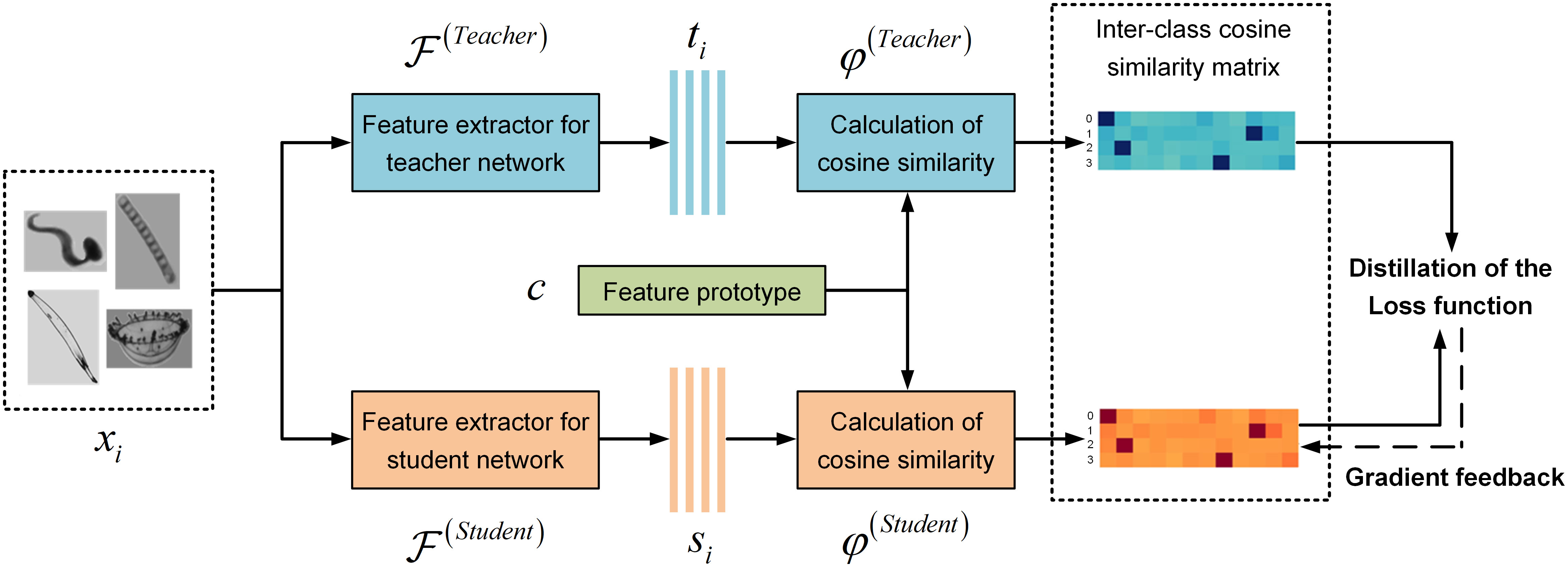
Figure 3 Process overview of the proposed PPD methods.

The inter-class similarity matrix of the teacher network was regarded as the expected knowledge, so we only updated the parameters of the student network to learn the distribution of inter-class similarity. This resulted in the gradual improvement of the recognition accuracy of the student network. Compared with the classical knowledge distillation methods, the advantages of our method are as follows: (1) The selection of feature prototype helps to avoid the interference of feature outliers. (2) Only one loss function relying on inter-class similarity is used, without extra calculation of classification loss. (3) There is no need to set hyperparameters $\alpha$, which reduces the impact of manual factors on performance.

2.2.2 Mathematic details of the model

The learning mechanism of neural network can be understood as the mapping from the sample space (input data) to the high-dimensional feature space. Using $x_i$ and $f_i$ to represent the sample and feature vectors, respectively, the cosine similarity between two feature vectors is defined as follows:

$\begin{array}{ll}{\text{σ}}_{i,j}=\frac{f_i{f}_j^T}{{\Vert f_i\Vert }_2{\Vert f_j\Vert }_2}& (3)\end{array}$

For classification tasks, the ideal situation is that the feature vectors of different classes are orthogonal to each other, and those of the same classes are toward the common direction, corresponding to 0 and 1 in similarity, respectively. The network is aimed at reducing the inter-class similarity and increasing the intra-class similarity. A trained network which satisfies the test standard is considered to satisfy the aforementioned requirements. The network can be regarded as a feature extractor$ℱ$to encode the sample vectors:

$\begin{array}{ll}{t}_i=ℱ(x_i)& (4)\end{array}$

for the class labeled by$k$, we calculate the means of all vectors $t_k$ in feature space ${\mathcal{T}}_k$ and normalize them by l₂-norm to obtain the feature prototype:

$\begin{array}{ll}\begin{array}{cc}{\mathit{\text{c}}}_k=\frac{{{\mathit{\text{t}}}^{\prime }}_k}{{\Vert {{\mathit{\text{t}}}^{\prime }}_k\Vert }_2}=\frac{{{\mathit{\text{t}}}^{\prime }}_k}{\sqrt{{\displaystyle \sum _{j=1}^D{({{\mathit{\text{t}}}^{\prime }}_{k,j})}^2}}},& {{\mathit{\text{t}}}^{\prime }}_k=\frac{1}{M_k}{\displaystyle \sum _{t_i\in {\mathcal{T}}_k}{t}_i}\end{array}& (5)\end{array}$

$\begin{array}{ll}C=\text{Concat}(c_1,c_2,\dots ,c_K)& (6)\end{array}$

where $M_k$ donates the number of vectors labeled by class $k$ and $D$ donates the dimension of $t_k$. Equation 6 is the matrix representation of the combination of all classes’ feature prototypes.

Furthermore, the inner product of the teacher feature $t_i$ (also standardized by l₂-norm), and the feature prototype $c_k$ is performed to obtain the cosine similarity distance, which is the expected knowledge in distillation, as shown in Equation 7. To simplify the calculation, the cosine similarity calculation between the teacher feature $t_i$ and all feature prototypes can be obtained in the form of matrices, as shown in Equation 8.

$\begin{array}{ll}{\text{φ}}_{i,k}=\frac{t_i{c}_k^T}{{\Vert t_i\Vert }_2}=\frac{{\displaystyle \sum _{j=1}^D{t}_{i,j}{c}_{k,j}}}{\sqrt{{\displaystyle \sum _{j=1}^D{t}_{i,j}^2}}}& (7)\end{array}$

$\begin{array}{ll}\text{Φ}(t_i)=\frac{t_i{C}^T}{{\Vert t_i\Vert }_2}=\frac{t_i{C}^T}{\sqrt{{\displaystyle \sum _{j=1}^D{(t_{i,j})}^2}}}& (8)\end{array}$

For the student network, the untrained encoder is considered unreliable. However, it can calculate the student feature $s_i$ initially. Using Equations 7, 8, we obtain Equations 9, 10 to calculate the cosine similarity of student features:

$\begin{array}{ll}{\text{φ}}_{i,k}=\frac{s_i{c}_k^T}{{\Vert s_i\Vert }_2}=\frac{{\displaystyle \sum _{j=1}^D{s}_{i,j}{c}_{k,j}}}{\sqrt{{\displaystyle \sum _{j=1}^D{s}_{i,j}^2}}}& (9)\end{array}$

$\begin{array}{ll}\text{Φ}(s_i)=\frac{s_i{C}^T}{{\Vert s_i\Vert }_2}=\frac{s_i{C}^T}{\sqrt{{\displaystyle \sum _{j=1}^D{(s_{i,j})}^2}}}& (10)\end{array}$

We calculate the MSE loss and use the gradient descent algorithm to guide the student network to learn the similarity between the individual samples encoded by the teacher network and finally improve the recognition ability of the lightweight networks. The loss function is expressed as follows:

$\begin{array}{ll}{ℒ}_{PPD-MSE}=\frac{1}{N}{\displaystyle \sum _{i=1}^N{\Vert \text{Φ}(t_i)-\text{Φ}(s_i)\Vert }_2^2}& (11)\end{array}$

2.3 Transformer models

Underwater plankton images are often acquired under suboptimal imaging conditions. Despite the complete extraction of ROIs, targets often remain visually unclear. A CNN model can continuously be iterated into a forward computing graph for feature extraction through gradient descent. The spatial perception of CNN is the regular expansion of receptive field with the convolutional layers increasing. This implies a fixed interaction mode of global and local information of the image and causes a trend of overfitting and parameter redundancy. Therefore, plagued with complex features and high requirements of data processing, new neural network architecture, that is, the Transformer was chosen to improve the recognition accuracy at the beginning of teacher networks’ training. This network architecture has demonstrated its strong performance over CNN in ecological automatic classification (Kyathanahally et al., 2022).

Transformer was proposed by Google in 2017 (Vaswani et al., 2017) and has achieved great success in the field of natural language processing (NLP). It employs a multi-head attention mechanism to extract features at any distance in the entire text, so that a single piece of information can flexibly implement multi-position and cross-scale interactive encodings. In 2020, Vision Transformer (ViT) was proposed (Dosovitskiy et al., 2020), and the encoder part of the initial Transformer was applied to extract image features. This scheme achieved the highest results in various computer vision (CV) tasks. To further incorporate the characteristics of image processing, the hierarchy of feature interactions in sub-regions of image (tokens) and their internal pixels were considered, which led to the proposal of Swin Transformer (Liu et al., 2021). This network shows better performance in characterization process and improves computational efficiency, which renders it potentially applicable to various fields.

This study focuses on the performance of Transformer architectures on the plankton taxonomic dataset (Section 2.1.3). We utilized several CNN and Transformer neural networks to evaluate the classification accuracy and computing speed. Furthermore, given the effectiveness of transfer learning (Pan and Yang, 2010) in plankton classification studies (Orenstein and Beijbom, 2017; Lumini and Nanni, 2019), we introduced transfer learning to provide pre-trained models (PTMs) for neural networks. These PTMs showed excellent performance in general CV scenarios, and their parameters experienced many iterations on large-scale public datasets. In some applications with specific requirements, these models can reach the accuracy by secondly training on the small datasets and fine-tuning the parameters. Under traditional training modes, the same accuracy needs a large amount of data and training times. The pre-training is beneficial to save computing resources and reduce data consumption.

2.4 Bilateral–Sobel edge enhancement

We proposed an edge enhancement method for fragile image texture to preprocess the images. The edge enhancement was divided into two steps: suppression of high-frequency noise and highlight of visual edge. The kernel of Bilateral filtering (Tomasi and Manduchi, 1998; Bhonsle et al., 2012) was used, and on the basis of Gaussian kernel which considers the spatial relationship of pixels, it pays extra attention to the value distribution of adjacent pixels. Therefore, Bilateral filtering can protect the weak edge while denoising, so we choose it as the denoising procedure. In an odd-order Bilateral filtering kernel, the weights of matrix are set as follows:

$\begin{array}{ll}{G}_{x,y}=\frac{1}{{\text{τ}}_G}\exp \left(-\frac{x^2+y^2}{2{\text{σ}}_G^2}\right)& (12)\end{array}$

$\begin{array}{ll}{W}_{x,y,u,v}=\frac{1}{{\text{τ}}_W}\exp \left(-\frac{{(I_{u+x,u+y}-I_{u,v})}^2}{2{\text{σ}}_W^2}\right)& (13)\end{array}$

where $(u,v)$ denotes the global position of the central pixel; $x$and$y$represent the local coordinates of adjacent pixels; ${\text{σ}}_G$ and ${\text{σ}}_W$ are the standard deviations of the normal distribution; ${\text{τ}}_G$ and ${\text{τ}}_W$ are weight coefficients applied to ensure the sum of the weights in the kernels are 1; and $I$ is the pixel value before processing. As one can see, in the spatial kernel $G$ and value kernel $W$, the closer the adjacent pixel to the central pixel in Euclidean distance and grayscale value, respectively, the greater its contribution to smoothing calculation. Furthermore, the final kernel function $B$ is the inner product of the two matrices.

The above design can prevent the smooth denoising from breaking slight and thin edges and, thus, preserve the complete foreground information within in-situ images. However, the foreground and background remain indistinguishable in case of close pixel values of areas. To extract the objects submerged into the background, we further applied the Sobel operator (Vincent and Folorunso, 2009) to completely separate the edge part in the gradient dimension for the images obtained after bilateral filtering. The gradient values in the two directions of images, $S_x$ and $S_y$ are calculated using standard Sobel kernels $D_x$ and $D_y$, respectively, and synthesize into the final result $S_{xy}$ through vector addition. The entire process is expressed as follows:

$\begin{array}{ll}\begin{array}{ccc}{D}_x=\left[\begin{array}{ccc}-1& 0& 1\\ -2& 0& 2\\ -1& 0& 1\end{array}\right],& D_y=\left[\begin{array}{ccc}-1& -2& -1\\ 0& 0& 0\\ 1& 2& 1\end{array}\right],& S_{xy}=\sqrt{S_x^2+S_y^2}\end{array}& (14)\end{array}$

After the gradient image $S_{xy}$ is obtained through the above steps, and it is used as input for steps (3) to (7) in the algorithm pipeline described in Section 2.1.1.

3 Results

In order to examine the effectiveness of proposed methods and their contribution to the performance of algorithm pipeline, in this part, we designed a set of experiments and present the results. The sequence of results is shown in the order of algorithm pipeline. In Section 3.1, the effects of Bilateral–Sobel edge enhancement on in-situ images from test dataset (Section 2.1.2) are shown. In Section 3.2, we compared the performance of CNN and Transformer families on taxonomic dataset (Section 2.1.3), and took the outstanding model as the teacher network to verify the superiority of the knowledge proposed distillation method over the traditional ones in Section 3.3. Finally, in Section 3.4, we validated the selected methods using test dataset, and paid extra attention to the results on gelatinous plankton (Medusae). These experiments were conducted on the same computing hardware, using an Intel Core i7-8750H processor, 16GB of RAM, and Nvidia GeForce GTX 1060 graphics cards.

3.1 Effects of Bilateral–Sobel edge enhancement

3.1.1 Visualization of Gaussian, Bilateral, and Sobel processing results

First, we compared Gaussian and Bilateral operators to filter an image of an individual of Medusae and evaluated the results of subsequent binarization. As shown in Figure 4A, the boundary on both sides of the upper part in the raw image is weakly connected. Upon the application of Gaussian filtering, as shown in Figure 4C, the concerned edge breaks, whereas Bilateral filtering retains the shape of the edge to the best extent (Figure 4B).

FIGURE 4

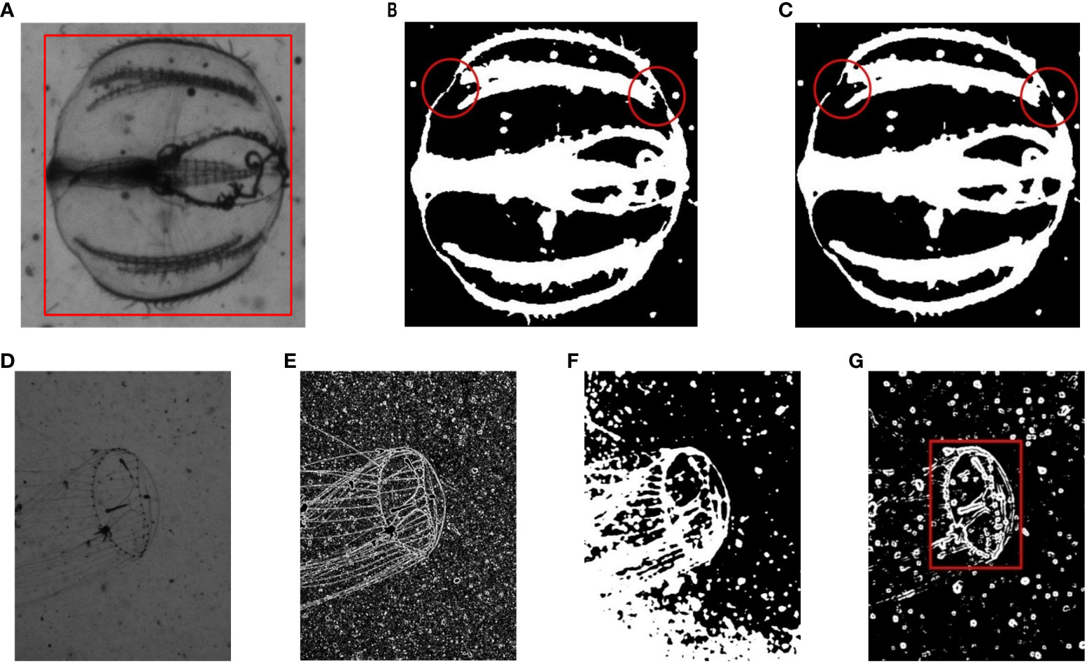
Figure 4 Visual evaluation of enhancement methods. (A) Before processing; (B) Bilateral filtering; (C) Gaussian filtering; (D) before processing; (E) operation by Sobel kernel only; (F) operation by Bilateral kernel only; and (G) operation by Bilateral and Sobel kernels; (B–G) experienced subsequent binarization.

Figures 4D–G show the independent and united results of the Bilateral and Sobel operators. As shown in Figure 4E, it is obvious that the single gradient calculation cannot suppress the high-frequency noise of the background. Although a single Bilateral filter can preserve the weak edges as much as possible while denoising, some too weak edges are still stick together with the background (Figure 4F). This will make some background regions be recognized as part of ROIs. Therefore, we used a combination of Bilateral–Sobel edge enhancement to perform a comprehensive operation in spatial, value, and gradient domains, so as to achieve complete segmentation of the target in binarization step.

3.1.2 Comparative experiments on edge enhancement

In order to quantitatively analyze the effect of Bilateral–Sobel edge enhancement and other preprocessing methods on target extraction, we used steps (1)–(5) of the algorithm pipeline described in Section 2.1.1 for target extraction. We used the find contours function in the OpenCV library for target extraction at step (5). In addition, we set the denoising and edge enhancement operations for step (2) as follows: no denoising and edge enhancement, only Gaussian filtering, only Bilateral filtering, combination of Gaussian filtering and Sobel gradient calculation, and combination of Bilateral filtering and Sobel gradient calculation. All experimental subjects were raw images from the dataset presented in Section 2.1.2. The evaluation indicators were the precision (the quantity ratio of complete ROIs to extracted ROIs) and recall (the quantity ratio of complete ROIs to the total targets), as well as the extraction speed [number of images processed by steps (1) to (5) within 1 s]. In in-situ images, some targets have blurry edges, which can easily cause edge breaks during the process of extraction, resulting in one target being divided into multiple ROIs. The complete ROI refers to the fact that the specific target does not have broken pixel connections, which means that the complete ROI does not share a target with other ROIs. The results present in Table 1 show that our preferred method exhibits the best extraction result, implying our edge enhancement renders the target much easier to be detected.

TABLE 1

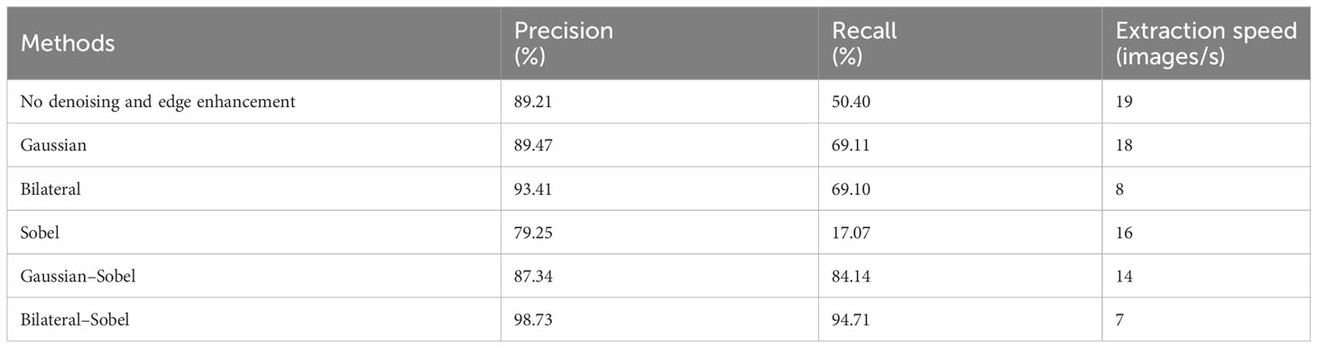
Table 1 Results of comparative experiments on edge enhancement.

3.2 Performance of CNN and Transformer schemes

In this section, we compared the performance of neural networks with extensive parameter volumes both in CNN and Transformer families. We demonstrated the test on the taxonomic dataset from South China Sea (Section 2.1.3). Furthermore, the effectiveness of the parameters pre-trained by the ImageNet dataset (Ridnik et al., 2021) was verified in the plankton classification task. In this experiment, MobileNet V2 (Sandler et al., 2018), ShuffleNet V2 (Ma et al., 2018), ResNet50, ResNet101, and ResNet152 (He et al., 2016) were selected from the CNN architectures; Swin-T (Liu et al., 2021), ViT-B (Dosovitskiy et al., 2020), and Swin-B (Liu et al., 2021) were selected from the Transformer architectures. We conducted two types of training modes: (1) direct training on the taxonomic dataset and (2) loading the pre-training model and then fine-tuning by the taxonomic dataset. The accuracy (the number of correctly classified samples divided by the total number of samples) results and the size (quantified as storage memories) of models are presented in Table 2. The CE loss function was used in the training process.

TABLE 2

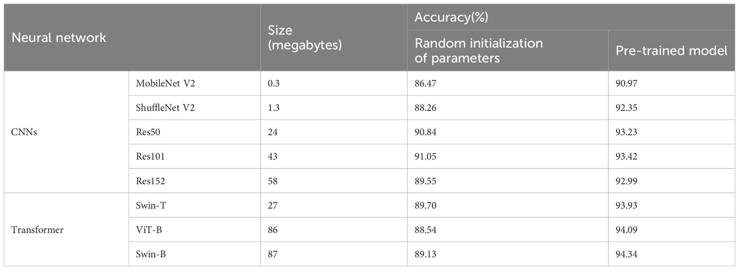
Table 2 Performance of different neural networks and training strategies on taxonomic dataset.

As shown in Table 2, the best performance is reached by pre-trained Swin-B with an accuracy of 94.34%. Furthermore, for both two network families, transfer learning yields higher accuracy than direct training. In addition, the performances of the Transformer variants are inferior to that of the CNN variants in direct training when the network is initialized by random parameters. Thus, the Transformer architectures may not be suitable for medium and small-scale datasets without any priori information, and its feature perception is not as experienced as the mode of CNNs in this case. However, pre-training may equivalently improve the amount of data in the source domain, and resulted in the Transformers’ performance exceeding that of the CNNs. We have discussed this situation at the end of this paper. From the results, we considered that the pre-trained Swin-B model stood out in the application of plankton classification and planned to integrate it into the following knowledge distillation algorithm.

3.3 Experimental results of the proposed knowledge distillation method

3.3.1 Comparison with classical knowledge distillation methods

The trained Swin-B model in Section 3.2 was selected as the teacher network to guide the convergence of student network. This model occupies storage of 87M and its reasoning speed is 26 targets per second. We compared the proposed knowledge distillation method with the other four classic technologies reported in recent years mentioned in Part 1, including: KD: knowledge distillation (Hinton et al., 2015); FitNet (Romero et al., 2014); SP: similarity preserving (Tung and Mori, 2019); CC: correlation congruence(Peng et al., 2019); and CE: cross-entropy (Ferdous et al., 2020). Five neural networks with different parameter volumes and reasoning speeds were used as student networks. In addition, a multi-layer perceptron structure was used to match the output dimensions of student networks with the teacher network. Using the dataset described in Section 2.1.3, the final results of the five methods are presented in Table 3.

TABLE 3

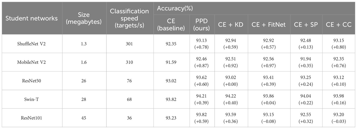
Table 3 Comparative experimental results of different knowledge distillation methods.

The column of CE (baseline) represents classification training by using cross entropy loss function, without any knowledge distillation processes. The accuracy achieved in this column is taken as the baseline. As shown in the table, the proposed method (PPD) guides five student networks to improve the accuracy (number of correctly classified samples divided by the total number of samples), and achieves a higher or nearly equal increase compared with other methods. Moreover, the accuracy of ShuffleNet V2 with the help of PPD (93.13%) exceeds ResNet50 under traditional training (93.02%), whereas the parameter volume of the former is only 5% of the latter. This implies that our method can make the lightweight network show better recognition ability than large scale neural networks under traditional training.

All networks use Adam (Kingma and Ba, 2014) as the training optimizer. After each epoch of training and validation, the model parameters were saved once, and the current highest validation accuracy rate was recorded. If the highest validation accuracy rate remained unchanged for several epochs, the learning rate was reduced (the learning rates of ShuffleNet V2 and MobileNet V2 are reduced by 10 times; the learning rate of ResNet50, Swin-T and ResNet101 are reduced by four times.) and load the model parameters corresponding to the highest accuracy to continue the training.

3.3.2 Evaluation of different loss functions

One of the key points of the proposed method is the similarity enhancement of feature descriptions between teacher and student networks. In the experiments above, we used MSE as the loss function (Equation 11), which usually appears in regression tasks. In this section, we discussed other two common loss functions from classification tasks: the CE and KL divergence loss functions. ShuffleNet V2 and Swin-T with better performance in Table 3 were used as the student network and the results are presented in Table 4. It can be seen that the MSE was most applicable to our frameworks, implying that the learning of our defined knowledge should be regarded as a regression process. The reasons for the poor performance of the other two loss functions can be inferred as follows: The dot product of the similarity matrix and the one-hot coding resulted in the loss of the relationship information between classes, leading the degradation of the final effect; Because the features are processed by the l₂-norm during distillation, the value of similarity was distributed in a narrow range of [−1,1], and both CE and KL loss need to perform softmax operation on the outputs similarity value; thus, they caused the output probability distribution being excessively smooth and weakening the positive response of intra-class features.

TABLE 4

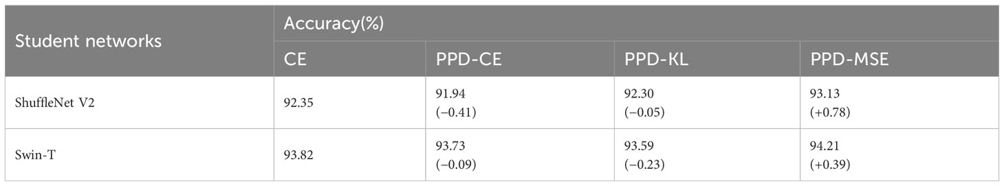
Table 4 Effect of PPD method with different loss functions.

3.4 Examination of the update of algorithm pipeline

We finally demonstrated the experiments to examine the upgrade of algorithm pipeline, hoping that the quality of image processing can reach excellent performance. As for the segmentation stage, the Bilateral–Sobel edge enhancement aided in the target extraction and location. In the stage of classification, we further verified the three student networks that performed well in the previous experiments (Section 3.3.1) and the selected teacher network, Swin-B (Section 2.1.2). In addition, Medusae is difficult in target extraction and classification due to its weak edge connection and similar gray value to background and so forth, so we paid extra attention to the detection effect of Medusae. The results are presented in Table 5.

TABLE 5

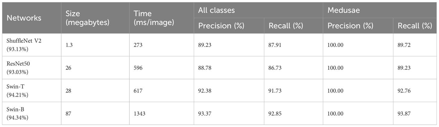
Table 5 Performance of different models on test dataset.

It can be summarized that the trained Swin-B still exhibits the best performance. However, the model is very large and the processing time is more than 1 s, which is not suitable for terminal deployment. ShuffleNet V2 and Swin-T, which were guided by Swin-B with the proposed PPD, also perform better. The lightweight ShuffleNet V2 exhibits better performance than ResNet50 and requires only 273 milliseconds to process one in-situ image. Swin-T exhibits a better accuracy and also satisfies the acceptable storage capacity and processing speed.

4 Discussion

4.1 Deep understanding of the operations on plankton features

We applied knowledge distillation and updated the algorithm pipeline to pursue better detection and recognition effects of targets in plankton in-situ images. Here, it should be emphasized that our design inspirations of the methods focus on the mathematical operations on plankton features. In order to explain understandably, we define two temporary terms of plankton ROIs: (1) regional features, which represent the relative spatial position of ROIs in the background, and (2) classification features, which represent the class properties (including shape, texture features, etc.). Regional features and classification features are the features of ROIs in space and as objects, respectively. According to the steps of algorithm pipeline, we enhance the regional features and extract the classification features.

Bilateral–Sobel edge enhancement enhances the regional features of targets and makes them be easily separated. In the previous segmentation tasks, it is challenged to distinguish the targets, interference noise, and chaotic background. For example, as for gelatinous plankton, their narrow edges of and dense noises possess the same spatial frequency, and the gray scale of interest pixel region and background are visually fused. Therefore, ROIs, noises, and background are mixed in regional features and cannot be separated by single methods such as filtering. To solve these problems, we combined the distinguishing abilities of the filter kernel functions (Bilateral–Sobel operator) in the spatial, value, and gradient domains, to reduce the correlation of the mixed region features. In addition, the subsequent separation can be easily realized to obtain the complete ROIs. The verified experiments of the complete extraction reached the accuracy and recall rate of 98.73% and 94.73%, respectively.

For the classification steps, the discrimination of classification features of extracted ROIs is weak. However, neural networks can be used to map them to high-dimensional expressions, which can be easily distinguished. According to the experimental results, the best way for us to demonstrate the extraction of classification features is to fine-tune the calculation model of the pre-trained Swin-B on the taxonomic dataset, with the best accuracy of 94.34%. Moreover, the multi-head attention mechanism of the Transformer variants implements global and long-distance perception, which is different from the layer-by-layer expansion of CNN. The Transformer variants require sufficient training data, and the performance of the Transformers was inferior to that of CNNs without transfer learning. However, the perception mechanisms of neural network to ordinary images and in-situ images are naturally similar; thus, the application of the pre-training network is equivalent to increasing the size of the dataset. Consequently, the Transformer variants can fully explore their potentials. To illustrate this inference, we used principal components analysis (PCA) to compress the output features from Swin-B before and after fine-tuning to two-dimensional representations, as shown in Figure 5. The network pre-trained by large ordinary image datasets exhibits a certain ability to distinguish the plankton targets. After transfer learning, it can further realize the feature clustering in small datasets and make each class region preserve sufficient feature distance. Therefore, the method we adopted has the potential to be applied in various specific scenarios.

FIGURE 5

Figure 5 Visual evaluation of the ability to distinguish features before (A) and after (B) fine-tuning of the pre-training model.

Knowledge distillation is to transplant the extraction ability of classification features. Here, we discuss the characteristics of the proposed PPD method, classical knowledge distillation method, and traditional supervised learning. For the classification tasks, traditional supervised learning utilizes the cross-entropy loss to push the outputs close to the extreme values of 1 and 0. Whereas, the classical knowledge distillation methods attempt to learn the information of probability distribution output by the teacher networks and promote the student networks’ perception of inter-class similarity. The proposed PPD method demonstrates the similarity calculation of classification features via interactions between an independent sample and a complete class. Our distillation mode combined intermediate feature learning with the generation of classification probabilities by using inter-class similarity. So, the gradient descent can simultaneously perform feature learning and supervised classification. The feature prototype extracted from the teacher network Swin-B and the sample features output from the teacher network were compressed into two-dimensional representation through PCA, and the results are shown in Figure 6. It can be seen that the feature prototypes are located in the centers of each cluster, which fully have the enough ability to express the features of each class. More importantly, some individual outlier features do not have obvious influences on the feature prototypes. Therefore, it can be seen that the average features as the characteristic prototypes are in line with the mathematical expectation. The interference from an outlier value is avoided and the damage of noise data to the classification performance is reduced. The proposed knowledge distillation method was tested through sufficient comparative experiments and obtained satisfactory results, and our novel method can be considered in wide range of applications.

FIGURE 6

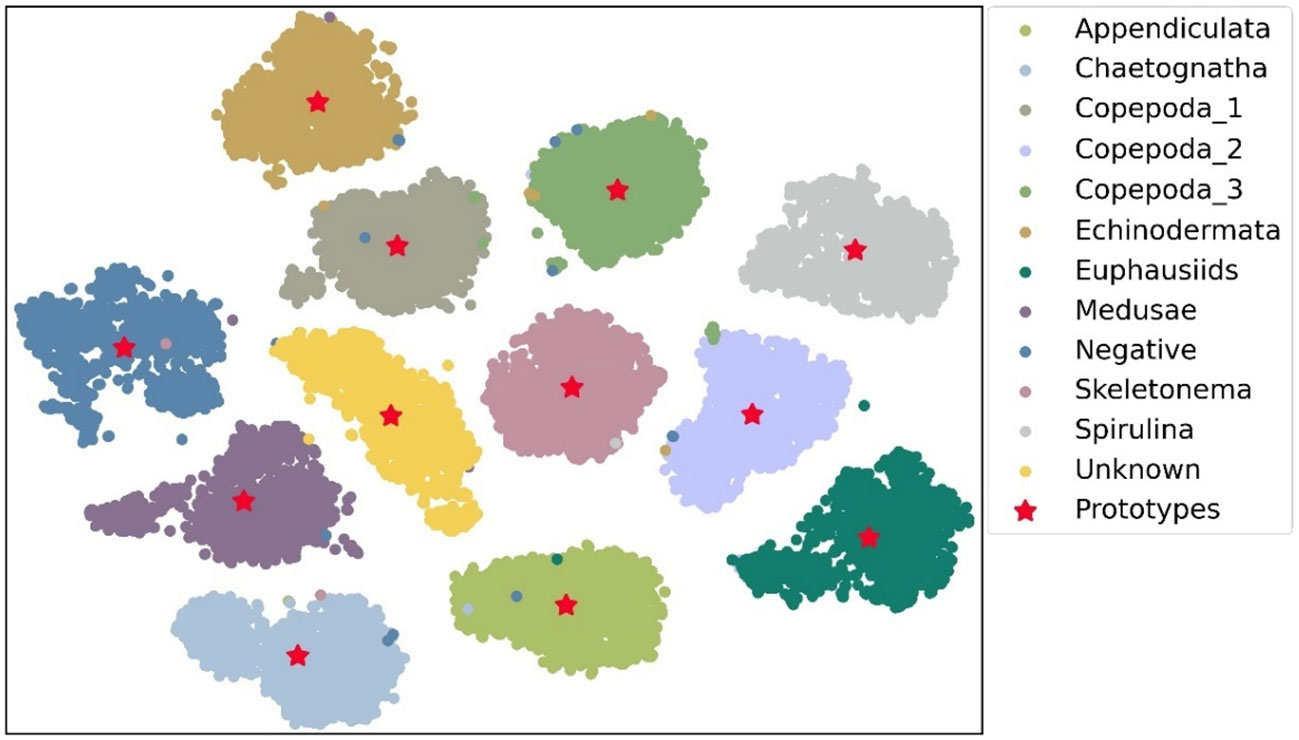
Figure 6 The visualization results of the feature prototype and the features of each sample output by the teacher network.

4.2 Prospects for the development of in-situ monitoring

According to extensive experiments conducted above, our proposed methods have updated the algorithm pipeline and achieved satisfactory results on the test dataset. The lightweight neural networks can reach high accuracy and be appropriate to be deployed. The excellent effects and the practicability of Transformer variants and the proposed PPD method are verified in the plankton in-situ images.

The image processing for the current algorithm pipeline can be developed continuously. We are considering designing end-to-end deep learning object detection frameworks in our systems as many works have done in CV field. In addition, as the qualities of in-situ images are generally not ideal, it is necessary to build a large-scale plankton object detection dataset in the next period. Furthermore, unsupervised learning for plankton classification may be discussed and unlabeled data may be used to improve the representation ability of the models. In addition, the use of computer programs to assist in labeling and cleaning in-situ data are also expected to rapidly expand the database. For recognition tasks, compared with CNN in most recognition tasks, Transformer has not been saturated with the growth of network parameters and dataset size (Vaswani et al., 2017). Therefore, we still believe that with the continuous surge of underwater data, the Transformer will have a broader prospect in plankton monitoring applications. In terms of model compression, in addition to knowledge distillation, pruning is another kind of effective method. In recent years, researchers have explored how to effectively combine the two methods, and related works have been carried out (Park and No, 2022; Liang et al., 2023), revealing the excellent effect that the combination schemes can bring.

In addition, the quality of dataset at the sensor side should be also focused on, especially the development of high-quality underwater optical imaging system. The adaptability of the imaging systems to the coastal, estuarine, and other complex water areas especially with high turbidity and water velocity need to be improved. A sincere suggestion is to introduce new hardware aids from the perspective of optical design, and the high quality of the source information will greatly reduce the difficulty of subsequent image processing.

4.3 Conclusions

This study proposed and demonstrated a novel knowledge distillation method and synchronously equipped new algorithm system for target detection and recognition regarding in-situ images of plankton. The experiments were based on the datasets captured by the experienced underwater imaging system PlanktonScope. Furthermore, the method expanded the analytical ability to gelatinous plankton, which has been a challenge till now, and achieved high recognition recall rate and short processing time. Especially, a new inter-class similarity distillation algorithm based on feature prototypes was proposed. For the first time, we used the similarity assessment of features among independent samples and complete classes as a regression task to realize knowledge distillation. Consequently, better performance was shown on the taxonomic dataset of plankton. Moreover, through experiments and comparisons with classical methods, we formed the final update of algorithm pipeline and discussed the work results and inner principle. The improvement of optical imaging and the exploration in image processing in the field of deep learning will be the two main focus points of future work.

Data availability statement

The data and the code used for algorithm implementation will be made available by the authors, without undue reservation.

Author contributions

JY, ZC, and YL completed the background investigation, method design, and experiments, and led the writing of the paper. KC provided materials of the original algorithm pipeline and participated in the comparative experiments. HB and XC provided valuable suggestions for the whole work and revised the paper. All authors contributed to the article and approved the submitted version.

Funding

This work was supported in part by the National Key Research and Development Program of China (No. 2017YFC1403602) and the Shenzhen Science and Technology Innovation Program (Nos. KCXFZ20211020163557022, JSGG20191129110031632, JCYJ20170412171011187), and the National Natural Science Foundation of China (Nos. 61527826, 51735002), and the Major Scientific and Technological Innovation Project of the Shandong Provincial Key Research and Development Program (2019JZZY020708).

Acknowledgments

The authors express their sincere gratitude to the reviewers and editors who provided valuable comments and assistance for the publication.

Conflict of interest

The authors declare that the research was conducted in the absence of any commercial or financial relationships that could be construed as a potential conflict of interest.

Publisher’s note

All claims expressed in this article are solely those of the authors and do not necessarily represent those of their affiliated organizations, or those of the publisher, the editors and the reviewers. Any product that may be evaluated in this article, or claim that may be made by its manufacturer, is not guaranteed or endorsed by the publisher.

References

Azani N., Ghaffar M., Suhaimi H., Azra M., Hassan M., Jung L., et al. (2021). “The impacts of climate change on plankton as live food: A review,” in IOP Conf. Ser.: Earth Environ. Sci. (Virtual, Indonesia: IOP Science) 869(1), 012005. doi: 10.1088/1755-1315/869/1/012005

CrossRef Full Text | Google Scholar

Benfield M. C., Shaw R. F., Schwehm C. J. (2000). Development of a vertically profiling, high-resolution, digital still camera system. Louisiana State Univ. Baton Rouge Dept Oceanogr. Coast. Sci. 2000. doi: 10.21236/ADA609777

CrossRef Full Text | Google Scholar

Bhonsle D., Chandra V., Sinha G. R. (2012). “Medical image denoising using bilateral filter,” in Int. J. Image Graph. Sign. Proces (MECS Publisher) 4(6). 36–43. doi: 10.5815/ijigsp.2012.06.06

CrossRef Full Text | Google Scholar

Bi H., Cook S., Yu H., Benfield M. C., Houde E. D. (2013). Deployment of an imaging system to investigate fine-scale spatial distribution of early life stages of the ctenophore Mnemiopsis leidyi in Chesapeake Bay. J. Plankton Res. 35 (2), 270–280. doi: 10.1093/plankt/fbs094

CrossRef Full Text | Google Scholar

Bi H., Guo Z., Benfield M. C., Fan C., Ford M., Shahrestani S., et al. (2015). A semi-automated image analysis procedure for in situ plankton imaging systems. PloS One 10 (5), e0127121. doi: 10.1371/journal.pone.0127121

PubMed Abstract | CrossRef Full Text | Google Scholar

Bi H., Song J., Zhao J., Liu H., Cheng X., Wang L., et al. (2022). Temporal characteristics of plankton indicators in coastal waters: High-frequency data from PlanktonScope. J. Sea. Res. 189, 102283. doi: 10.1016/j.seares.2022.102283

CrossRef Full Text | Google Scholar

Braz J. E. M., Dias J. D., Bonecker C. C., Simoes N. R. (2020). Oligotrophication affects the size structure and potential ecological interactions of planktonic microcrustaceans. Aquat. Sci. 82 (3), 1–10. doi: 10.1007/s00027-020-00733-z

PubMed Abstract | CrossRef Full Text | Google Scholar

Brun P., Vogt M., Payne M. R., Gruber N., O'brien C. J., Buitenhuis E. T., et al. (2015). Ecological niches of open ocean phytoplankton taxa. Limnol. Oceanogr. 60 (3), 1020–1038. doi: 10.1002/lno.10074

CrossRef Full Text | Google Scholar

Buskey E. J., Hyatt C. J. (2006). Use of the FlowCAM for semi-automated recognition and enumeration of red tide cells (Karenia brevis) in natural plankton samples. Harmful Algae 5 (6), 685–692. doi: 10.1016/j.hal.2006.02.003

CrossRef Full Text | Google Scholar

Campbell R. W., Roberts P. L., Jaffe J. (2020). The Prince William Sound Plankton Camera: a profiling in situ observatory of plankton and particulates. ICES J. Mar. Sci. 77 (4), 1440–1455. doi: 10.1093/icesjms/fsaa029

CrossRef Full Text | Google Scholar

Cowen R. K., Guigand C. M. (2008). In situ ichthyoplankton imaging system (ISIIS): system design and preliminary results. Limnol. Oceanogr.-Meth. 6 (2), 126–132. doi: 10.4319/lom.2008.6.126

CrossRef Full Text | Google Scholar

Davis C. S., Gallager S. M., Marra M., Stewart W. K. (1996). Rapid visualization of plankton abundance and taxonomic composition using the Video Plankton Recorder. Deep-Sea Res. Pt. II 43 (7-8), 1947–1970. doi: 10.1016/S0967-0645(96)00051-3

CrossRef Full Text | Google Scholar

Dosovitskiy A., Beyer L., Kolesnikov A., Weissenborn D., Zhai X., Unterthiner T., et al. (2020). An image is worth 16x16 words: Transformers for image recognition at scale. doi: 10.48550/arxiv.2010.11929

CrossRef Full Text | Google Scholar

Fan A., Stock P., Graham B., Grave E., Gribonval R., Jegou H., et al. (2020). Training with quantization noise for extreme model compression. arXiv preprint arXiv. doi: 10.48550/arXiv.2004.07320

CrossRef Full Text | Google Scholar

Ferdous R. H., Arifeen M. M., Eiko T. S., Mamun S. A. (2020). “Performance analysis of different loss function in face detection architectures,” in Proc. Int. Conf. Trends in Comput. Cognit. Eng. 659–669. doi: 10.1007/978-981-33-4673-4_54

CrossRef Full Text | Google Scholar

Gorsky G., Picheral M., Stemmann L. (2000). Use of the Underwater Video Profiler for the study of aggregate dynamics in the North Mediterranean. Estuar. Coast. Shelf Sci. 50 (1), 121–128. doi: 10.1006/ecss.1999.0539

CrossRef Full Text | Google Scholar

Guo B., Yu J., Liu H., Xu W., Hou R., Zheng B. (2018). Miniaturized in situ dark-field microscope for in situ detecting plankton. Ocean Opt. Inf. Technol. 10850, 243–250. doi: 10.1117/12.2505639

CrossRef Full Text | Google Scholar

He K., Zhang X., Ren S., Sun J. (2016). “Deep residual learning for image recognition,” in Proc. IEEE Conf. Comput. Vis. Pattern Recognit. (Las Vegas, USA: IEEE), 770–778.

Google Scholar

Hermand J. P., Randall J., Dubois F., Queeckers P., Yourassowsky C., Roubaud F., et al. (2013). “In-situ holography microscopy of plankton and particles over the continental shelf of Senegal,” in 2013 Ocean Elec. (SYMPOL). (Kochi, India: IEEE), 1–10. doi: 10.1109/SYMPOL.2013.6701926

CrossRef Full Text | Google Scholar

Hinton G., Vinyals O., Dean J. (2015). Distilling the knowledge in a neural network. doi: 10.48550/arxiv.1503.02531

PubMed Abstract | CrossRef Full Text | Google Scholar

Kingma D. P., Ba J. (2014). Adam: a method for stochastic optimization. arXiv [Preprint] arXiv.1412.6980.

Google Scholar

Kyathanahally S. P., Hardeman T., Merz E., Bulas T., Reyes M., Isles P., et al. (2021). Deep learning classification of lake zooplankton. Front. Microbiol 12. doi: 10.3389/fmicb.2021.746297

CrossRef Full Text | Google Scholar

Kyathanahally S. P., Hardeman T., Reyes M., Merz E., Bulas T., Brun P., et al. (2022). Ensembles of data-efficient vision transformers as a new paradigm for automated classification in ecology. Sci. Rep. 12 (1), 18590. doi: 10.1038/s41598-022-21910-0

PubMed Abstract | CrossRef Full Text | Google Scholar

Li X., Cui Z. (2016). Deep residual networks for plankton classification. Oceans 2016 MTS/IEEE Monterey IEEE, 1–4. doi: 10.1109/OCEANS.2016.7761223

CrossRef Full Text | Google Scholar

Li Y., Guo J., Guo X., Zhao J., Yang Y., Hu Z., et al. (2021). Toward in situ zooplankton detection with a densely connected YOLOV3 model. Appl. Ocean Res. 114, 102783. doi: 10.1016/j.apor.2021.102783

CrossRef Full Text | Google Scholar

Liang C., Jiang H., Li Z., Tang X., Yin B., Zhao T., et al (2023). HomoDistil: homotopic task-agnostic distillation of pre-trained transformers. arXiv preprint arXiv: 2302.09632. doi: 10.48550/arxiv.2302.09632

CrossRef Full Text | Google Scholar

Liu Z., Lin Y., Cao Y., Hu H., Wei Y., Zhang Z., et al. (2021). “Swin transformer: Hierarchical vision transformer using shifted windows,” in Proc. Proc. IEEE Int. Conf. Comput. Vis. (Montreal, Canada: IEEE), 10012–10022.

Google Scholar

Lumini A., Nanni L. (2019). Deep learning and transfer learning features for plankton classification. Ecol. Inform. 51, 33–43. doi: 10.1016/j.ecoinf.2019.02.007

CrossRef Full Text | Google Scholar

Luo J. Y., Irisson J. O., Graham B., Guigand C., Sarafraz A., Mader C., et al. (2018). Automated plankton image analysis using convolutional neural networks. Limnol. Oceanogr.-Meth 16 (12), 814–827. doi: 10.1002/lom3.10285

CrossRef Full Text | Google Scholar

Lv Z., Zhang H., Liang J., Zhao T., Xu Y., Lei Y. (2022). Microalgae removal technology for the cold source of nuclear power plant: A review. Mar. pollut. Bull. 183, 114087. doi: 10.1016/j.marpolbul.2022.114087

PubMed Abstract | CrossRef Full Text | Google Scholar

Ma N., Zhang X., Zheng H.-T., Sun J. (2018). “Shufflenet v2: Practical guidelines for efficient cnn architecture design,” in Proc. Eur. Conf. Comput. Vis. (Munich, Germany: Springer), 116–131.

Google Scholar

Marini S., Fanelli E., Sbragaglia V., Azzurro E., Del Rio Fernandez J., Aguzzi J. (2018). Tracking fish abundance by underwater image recognition. Sci. Rep. 8 (1), 1–12. doi: 10.1038/s41598-018-32089-8

PubMed Abstract | CrossRef Full Text | Google Scholar

Orenstein E. C., Beijbom O. (2017). “Transfer learning and deep feature extraction for planktonic image data sets,” in IEEE Winter Conf. App. Comput. Vis. (Santa Rosa, USA: IEEE), doi: 10.1109/WACV.2017.125

CrossRef Full Text | Google Scholar

Orenstein E. C., Kenitz K. M., Roberts P. L. D., Franks P. J. S., Jaffe J. S., Barton A. D. A. (2020). Semi-and fully supervised quantification techniques to improve population estimates from machine classifiers. Limnol. Oceanogr.-Meth. 18 (12), 739–753. doi: 10.1002/lom3.10399

CrossRef Full Text | Google Scholar

Otsu N. (1979). A threshold selection method from gray-level histograms. IEEE Tran. Syst. Man Cybern. 9 (1), 62–66. doi: 10.1109/TSMC.1979.4310076

CrossRef Full Text | Google Scholar

Pan S. J., Yang Q. (2010). “A survey on transfer learning,” in IEEE Tran. Knowl. Data Eng. (IEEE). Vol. 22. 1345–1359. doi: 10.1109/TKDE.2009.191

CrossRef Full Text | Google Scholar

Park J., No A. (2022). “Prune your model before distill it,” in Proc. Eur. Conf. Comput. Vis. (Tel-Aviv, Israel: Springer), 120–136.

Google Scholar

Peng B., Jin X., Liu J., Li D., Wu Y., Liu Y., et al. (2019). “Correlation congruence for knowledge distillation,” in Proc. IEEE Int. Conf. Comput. Vis. (Seoul, South Korea: IEEE), 5007–5016.

Google Scholar

Piredda R., Tomasino M. P., D'Erchia A. M., Manzari C., Pesole G., Montresor M., et al. (2017). Diversity and temporal patterns of planktonic protist assemblages at a Mediterranean Long Term Ecological Research site. FEMS Microbiol. Ecol. 93 (1). doi: 10.1093/femsec/fiw200

PubMed Abstract | CrossRef Full Text | Google Scholar

Ridnik T., Ben-baruch E., Noy A., Zelnik-manor L. (2021). Imagenet-21k pretraining for the masses. doi: 10.48550/arxiv.2104.10972

CrossRef Full Text | Google Scholar

Romero A., Ballas N., Kahou S. E., Chassang A., Gatta C., Bengio Y. (2014). Fitnets: Hints for thin deep nets. doi: 10.48550/arxiv.1412.6550

CrossRef Full Text | Google Scholar

Said K. A. M., Jambek A. B., Sulaiman N. (2016). A study of image processing using morphological opening and closing processes. Int. J. Control Theor. App. 9 (31), 15–21.

Google Scholar

Sandler M., Howard A., Zhu M., Zhmoginov A., Chen L.-C. (2018). “Mobilenetv2: Inverted residuals and linear bottlenecks,” in Proc. IEEE Conf. Comput. Vis. Pattern Recognit. (Salt Lake City, USA: IEEE), 4510–4520.

Google Scholar

Song J., Bi H., Cai Z., Cheng X., He Y., Benfield M. C., et al. (2020). Early warning of Noctiluca scintillans blooms using in-situ plankton imaging system: an example from Dapeng Bay, PR China. Ecol. Indic. 112, 106123. doi: 10.1016/j.ecolind.2020.106123

CrossRef Full Text | Google Scholar

Suzuki S. (1985). Topological structural analysis of digitized binary images by border following. Comput. Gr. Image Process. 30 (1), 32–46. doi: 10.1016/0734-189X(85)90016-7

CrossRef Full Text | Google Scholar

Tanaka H., Kunin D., Yamins D. L. K., Gnguli S. (2020). Pruning neural networks without any data by iteratively conserving synaptic flow. Proc. Adv. Neural Inf. Process. Syst. 33, 6377–6389. doi: 10.48550/arXiv.2006.05467

CrossRef Full Text | Google Scholar

Tomasi C., Manduchi R. (1998). “Bilateral filtering for gray and color images,” in 6th Int. Conf. Comput. Vis. (Mumbai, India: IEEE). doi: 10.1109/ICCV.1998.710815

CrossRef Full Text | Google Scholar

Tung F., Mori G. (2019). “Similarity-preserving knowledge distillation,” in Proc. IEEE Int. Conf. Comput. Vis. (Seoul, South Korea: IEEE), 1365–1374.

Google Scholar

Vaswani A., Shazeer N., Parmar N., Uszkoreit J., Jones L., Gomez A., et al. (2017). Attention is all you need. Proc. Adv. Neural Inf. Process. Syst. 30. doi: 10.48550/arXiv.1706.03762

CrossRef Full Text | Google Scholar

Vincent O. R., Folorunso O. (2009). “A descriptive algorithm for sobel image edge detection,” in Proc. Inf. Sci. IT Educ. Conf, Vol. 40. 97–107.

Google Scholar

Wang Y., Liu Y., Guo H., Zhang H., Li D., Yao Z., et al. (2022). Long-term nutrient variation trends and their potential impact on phytoplankton in the southern Yellow Sea, China. Acta Oceanol. Sin. 41 (6), 54–67. doi: 10.1007/s13131-022-2031-3

CrossRef Full Text | Google Scholar

Wu J., Wang Y., Wu Z., Veeraraghavan A., Lin Y. (2018). Deep k-means: Re-training and parameter sharing with harder cluster assignments for compressing deep convolutions. doi: 10.48550/arXiv.1806.09228

CrossRef Full Text | Google Scholar