The impact of environmental factors on the phytoplankton communities in the Western Pacific Ocean: HPLC-CHEMTAX approach

The distribution characteristics, biomass, and communities of phytoplankton in the western Pacific Ocean (WPO) were investigated using high-performance liquid chromatography (HPLC)-CHEMTAX analysis. The results revealed significant differences in the distribution of phytoplankton communities among different water masses in the WPO. Haptophytes were the dominant group, followed by Prochlorophytes, Cyanobacteria, Prasinophytes, and Diatoms. The distribution of phytoplankton communities was primarily determined by the level of nitrate, phosphate, and silicate, while temperature showed a negative correlation with major phytoplankton communities. In the 130°E section, the divergence caused by Halmahera Eddy (HE) and Mindanao Eddy (ME) provided the abundant nutrients, making them the primary environmental influence factor near the equator. This divergence brought relatively eutrophic deep seawater into the euphotic layer, resulting higher biomass of phytoplankton communities. In the 20°N section, the distribution of phytoplankton was mainly influenced by the invasion of Kuroshio Current and its offshore flow. Additionally, due to the low surface-to-volume ratios, microphytoplankton dominated the phytoplankton community in this section instead of nanophytoplankton or picophytoplankton. In summary, this study confirms previous findings on distribution characteristics of phytoplankton and provides new insights into the environmental and biological regulations of phytoplankton communities in the WPO.

Introduction

The western Pacific Ocean (WPO) is known for its complex hydrological system and ecosystem, with significant impacts on global climate, ocean circulation, biodiversity, and the atmosphere (Turk-Kubo et al., 2018). Despite its vast area, the WPO is characterized as an oligotrophic sea with low biomass (Ma et al., 2021). Seawater stratification, seafloor topography, atmosphere cycle are among the several factors that can cause oligotrophic characteristics (Zhang et al., 2012). As a complex region, the WPO is affected by numerous ocean eddies and currents. Previous studies have observed massive wind-driven ocean circulation in the WPO (Collins et al., 2010; Yuan et al., 2011), particularly within the western boundary currents, such as Kuroshio Current (KC), Mindanao Current (MC), North Equatorial Current (NEC), North Equatorial Counter Current (NECC), as well as a series of eddies, including Halmahera Eddy (HE) and Mindanao Eddy (ME) (Hu et al., 2015). These eddies and currents can significantly influence nutrient transport, seawater stratification, and anomalous water properties in the WPO. Additionally, Mindanao Dome, a large-scale thermal upwelling dome in the WPO (Masumoto and Yamagata, 1991), provides a stable system for the western boundary current (Suzuki et al., 2005). Monsoons and warm pool can also seasonally influence the sea surface temperature (SST) in the WPO for mass transportation and temperature control (Jia et al., 2018), playing an essential role in the heat budget and global ocean circulation.

As a result of its diverse hydrological activities and vast area, the WPO has been recognized as a critical region for the global carbon cycle (Waga et al., 2022), marine primary production, biodiversity, and other ecological processes (Lin et al., 2011). Marine phytoplankton play critical roles in regulating the efficiency of the biological carbon pump, contributing nearly half of primary production and serving as biomarkers (Field et al., 1998), the WPO is an important carbon sink for marine carbon cycle (Mori et al., 2021), and understanding phytoplankton communities and their distribution is essential to study the ecosystem functions in the WPO (Liu et al., 2021a). Several studies have indicated that eddies and currents can transport nutrients from deep layers into the euphotic layer, resulting in increased primary production (Zhang et al., 2012; Hong et al., 2014). Moreover, cyclonic eddies and other oceanic dynamic phenomenon can enhance phytoplankton production rates by raising the thermocline and providing more nutrients (Behrens et al., 2018). These marine processes determine the distribution of phytoplankton communities, which can serve as indicators of the valuation in the marine environment (Zhang et al., 2012; Paul et al., 2021).

Although various methods can be used to identify and enumerate phytoplankton communities, such as microscopy and photosensitive probes (Liu et al., 2021b; Song et al., 2022), these methods may not accurately identify picophytoplankton, which is the primary phytoplankton community in the WPO (Hong et al., 2014). To observe phytoplankton more efficiently, identifying the diagnostic pigments within phytoplankton cells is valuable to determine the biomass and distribution of phytoplankton communities (Wright and Jeffrey, 2006; Higgins et al., 2011; An et al., 2018), and chemical taxonomy (CHEMTAX) is a program that allocates diagnostic pigments into taxa of interest (Mackey et al., 1996). CHEMTAX is more efficient and accurate in identifying phytoplankton communities at the class level and has been widely used in marine ecosystem research (Wright et al., 2010; Swan et al., 2016; Nomaki et al., 2021; Wang et al., 2021; Hyun et al., 2022).

In this study, phytoplankton pigment samples were collected from two sections of the WPO in 2016. Unlike previous studies in this area that rarely focus on the distribution of phytoplankton communities or their interaction with environmental factors, this study enables for the analysis of phytoplankton communities over a large spatial coverage. The phytoplankton pigments were analyzed by high-performance liquid chromatography (HPLC) (Mackey et al., 1998). Based on the results of CHEMTAX analysis, this study aims to: (i) investigate diagnostic pigments of phytoplankton to reveal the impacts of currents and eddies on phytoplankton communities; (ii) explore the controlling factors for the temporal and spatial distribution of phytoplankton communities; and (iii) indicate the influence of phytoplankton biochemical processes on the distribution of phytoplankton communities.

Materials and methods

Study area and sample collection

Oceanographic sampling was performed onboard R/V KEXUE in the WPO from 28 September to 25 October 2016 (Figure 1). A total of 6 stations in the 20°N section and 18 stations in the 130°E section were investigated during the cruise. At each station, seawater samples were collected by using 12 L Niskin bottles equipped with a Sea-bird CTD (SBE 19 Plus) rosette sampler at seven depths (5 m, 25 m, 50 m, 75 m, 100 m, 150 m, and 200 m). Physical parameters, such as depth, salinity, and temperature, were also recorded in situ at the same time using the CTD sensors. For nutrients analysis, 100 ml of seawater was collected without filtered and directly refrigerated at -20° until laboratory analysis. For diagnostic pigment samples, 4-6 L per each sample was collected and filtered using GF/F filter (0.7 µm pore-size, Whatman), and the membrane was immediately frozen in liquid nitrogen prior until analysis in the laboratory (Zhang et al., 2019b).

FIGURE 1

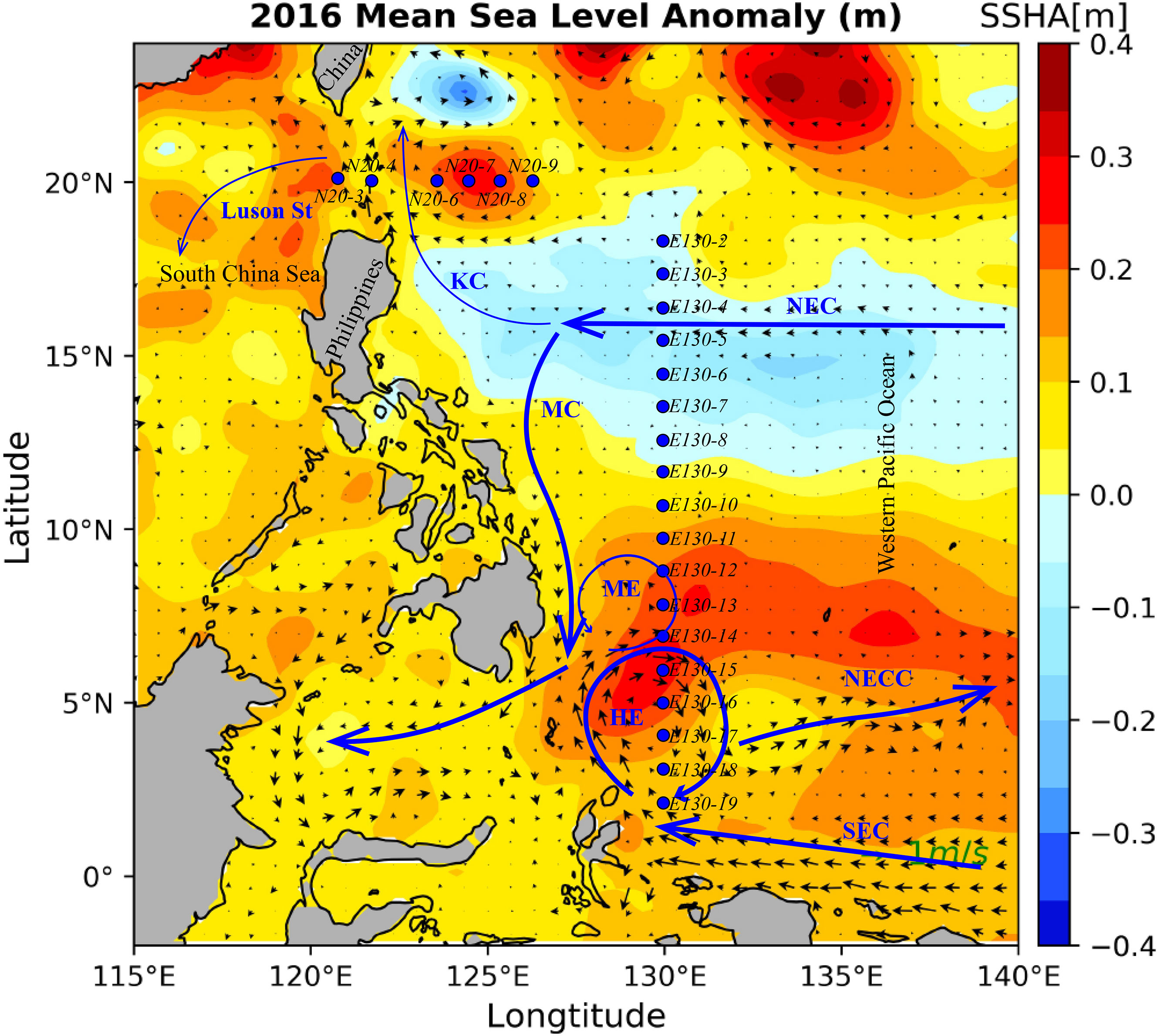
Figure 1 Map of sampling area with major surface currents and eddy system in the western Pacific Ocean (NEC, North Equatorial Current; KC, Kuroshio Current; MC, Mindanao Current; NECC, North Equatorial Counter Current; ME, Mindanao Eddy; HE, Halmahera Eddy). Blue dots are sampling stations and background plots the averaged sea surface height anomaly during the study period in 2016. The locations of eddies were identified using the gridded daily sea surface height anomaly (SSHA) with a spatial resolution of 0.25° acquired from the archiving validation and interpretation of satellite oceanography (https://www.aviso.altimetry.fr/en/home.html).

Sample analysis

Nutrient analysis

Nutrients, including dissolved inorganic ammonium (NH₄-N), nitrate (NO₃-N), nitrite (NO₂-N), phosphate (PO₄-P), and silicate (SiO₃-Si), were analyzed by Technicon Auto-Analyzer 3 (Bran + Luebbe, SEAL, Germany) based on continuous flow injection analysis (Grasshoff et al., 2009). The determination principles of nutrients were as follows: cadmium–copper reduction method for nitrate (detection limit: 0.015 µmol/L), azo dye formation method for nitrite (detection limit: 0.003 µmol/L), Berthelot reaction for ammonium (detection limit: 0.040 µmol/L), molybdenum blue method for phosphate (detection limit: 0.024 µmol/L) and silicate (detection limit: 0.030 µmol/L), respectively. In numerical terms, dissolved inorganic nitrogen (DIN) was the sum of ammonium, nitrite, and nitrate.

Diagnostic pigments analysis

Diagnostic pigments filters were extracted with 100% methanol for 1 h, then ultrasonic degassing for 30 s,(ice-bath), and finally preserved at -20° for 1 h. After preservation, all pigments extractions were filtered through 0.22 μm filters (Nylon) to remove impurities and mixed with 28 mmol/L of tetrabutylammonium acetate (TBAA). All the procedures were done under subdued light. Diagnostic pigments quantification was analyzed by the high-performance liquid chromatography system (Agilent Technologies 1260) with an Eclipse XDB C8 column (4.6×150 mm, 3.5 μm particle size) at a flow rate of 1 ml/min. The solvent included solvent A (methanol: 28 mmol/L TBAA (pH = 6.5), v/v = 70/30) and solvent B (100% methanol). Gradient elution procedure started with 80% solvent A and 20% solvent B, 30 min with 5% solvent A and 95% solvent B. The procedure ended at 50 min, and mobile phase ratio was 80% solvent A and 20% solvent B. The gradient eluting pigments were detected at 440 and 660 nm by the diode array detector. In our study, all the diagnostic pigments were identified and quantified using the pigment standards which were purchased from DHI Water and Environment, Hørsholm, Denmark. The following pigments were detected and quantified: Chlorophyll c3 (Chl c3), Chlorophyll c2 (Chl c2), Pheophorbide a (Phide a), Peridinin (Perid), 19’-but-fucoxanthin (But-fuco), Fucoxanthin (Fuco), Neoxanthin (Neo), Prasinoxanthin (Pras), Violaxanthin (Viola) 19’-hex-fucoxanthin (Hex-fuco), Diadinoxanthin (Diadino), Alloxanthin (Allo), Diatoxanthin (Diato), Zeaxanthin (Zea), Lutein (Lut), Chlorophyll b (Chl b), Divinyl Chlorophyll a (DV Chl a), Chlorophyll a (Chl a), Pheophytin a (Phytin a), α-carotene (α-car), and β-carotene (β-car).

Data analysis

Size-fractionated chlorophyll a calculation

Seven diagnostic pigments (Fuco, Perid, Allo, Hex-fuco, But-fuco, Zea, and Chl b) were used to calculated the contributions of microphytoplankton (fmicro), nanophytoplankton (fnano), and picophytoplankton (fpico) size-fractionated to total Chl a [Chl a] concentration (Uitz et al., 2006).

$\begin{array}{ll}fmicro=(1.41*[\text{Fu}co]+1.41*[\text{Perid}])/\text{ DP}& (1)\end{array}$

$\begin{array}{ll}fnano=(1.27*[\text{Hex}-\text{fuco}]+0.6*[\text{Allo}]+0.35*[\text{But}-\text{fuco}])/\text{ DP}& (2)\end{array}$

$\begin{array}{ll}fpico=(1.01*[\text{Chl b}]+0.86*[\text{Zea}])/\text{ DP} & (3)\end{array}$

Where DP is the weighted sum of the concentrations of seven diagnostic pigments, was calculated using equation (4):

$\begin{array}{ll}\begin{array}{c}\text{DP }=1.41*[\text{Fuco}]+1.41*[\text{Perid}]+1.27*[\text{Hex}-\text{fuco}]+0.6*[\text{Allo}]+\\ 0.35*[\text{But}-\text{fuco}]+1.01*[\text{Chl b}]+0.86*[\text{Zea}]\end{array}& (4)\end{array}$

The size-fractionated Chl a concentrations were then calculated as follows:

$\begin{array}{ll}\text{Micro}-\text{Chl }a=fmicro*[Chla]& (5)\end{array}$

$\begin{array}{ll}\text{Nano}-\text{Chl }a=fnano*[Chla]& (6)\end{array}$

$\begin{array}{ll}\text{Pico}-\text{Chl }a=fpico*[Chla]& (7)\end{array}$

CHEMTAX calculation

The phytoplankton community finds the most consistent phytoplankton community structure composition of the sample according to the factor analysis of CHEMTAX program and the steepest descent algorithm for the total Chlorophyll a (the sum of Chl a and DV Chl a in this study). According to the pigment composition of the WPO, the 14 initial diagnostic pigments ratio was applied to the WPO (Table 1) (Schlüter et al., 2011). The CHEMTAX results are mainly used to evaluate the dominant position of different phytoplankton communities. The CHEMTAX results of this project include 10 phytoplankton communities, namely, Chlorophytes, Chrysophytes, Cryptophytes, Cyanobacteria, Diatoms, Dinoflagellates, Euglenophytes, Haptophytes, Prasinophytes, and Prochlorophytes.

TABLE 1

Table 1 Preliminary pigment ratio of CHEMTAX analysis.

All contour maps were created using Ocean Data View (ODV) 5.6.2 (Schlitzer, 2002). Color scatter diagrams and linear regressions were processed by OriginPro 8.5.0. Redundancy analysis (RDA) and Person’s correlation coefficients were displayed to assess the corresponding relationship between the phytoplankton communities and the environmental parameters (e.g., temperature, salinity, and nutrients) and variances of phytoplankton communities in the different water masses, respectively.

Results

Hydrography and nutrients during the sampling period

According to the temperature-salinity diagram of water samples in survey area (Figure 2C), five water masses including ME (E130-10 to E130-14), HE (E130-17 to E130-19), NEC (E130-3 to E130-8), KC (N20-6 to N20-9), and SCS (N20-3 to N20-4) were identified. Due to high dispersion, other stations were classified as interval stations. Water temperature within upper the 200 m varied from 16° to 30° (Figure 2A), and salinity ranged from 33.5 to 35.5 (Figure 2B). The temperature exhibited relative stratification, with higher values above 100 m and lower values below 100 m. Similarly, the salinity stratification displayed in the upper layer was higher than that in the deeper layer.

FIGURE 2

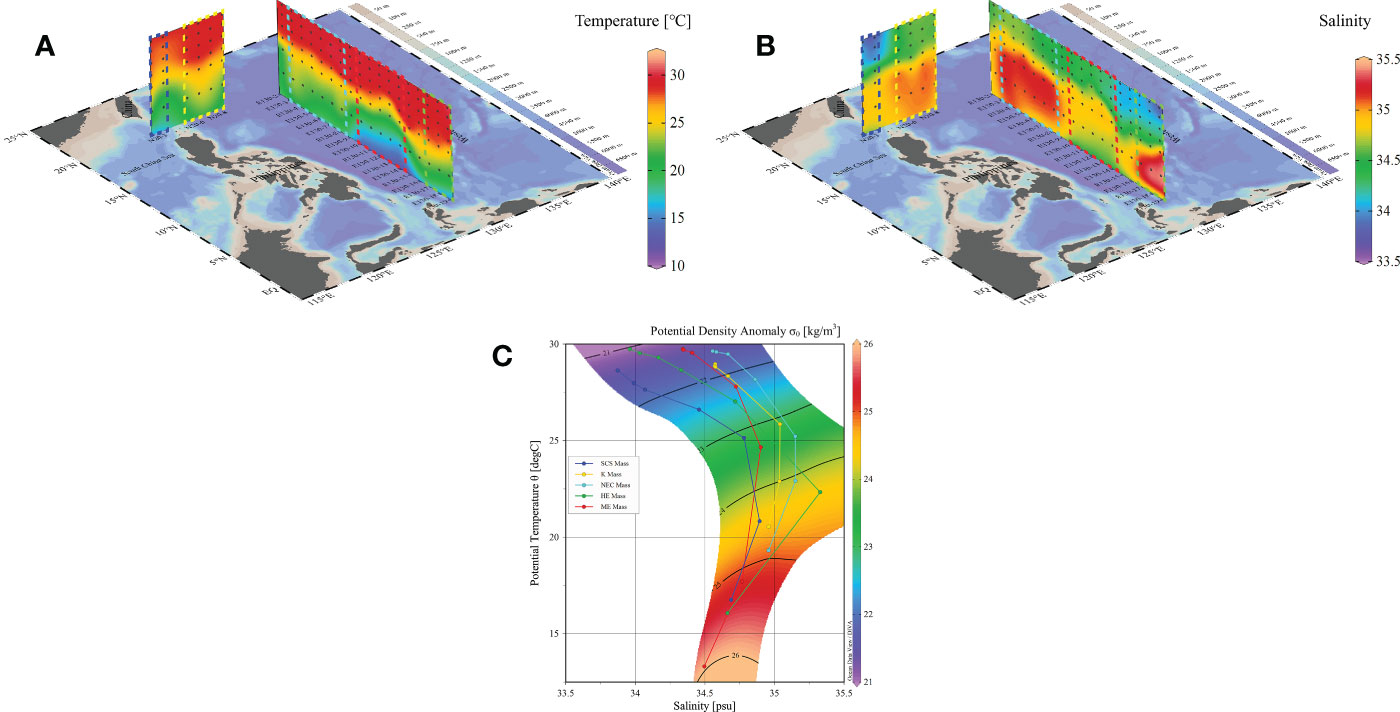
Figure 2 Diagram of temperature distribution (A), salinity distribution (B), and temperature-salinity (S-T) (C) during the sample period in the WPO.

In the 20°N section, a colder upwelling invaded the upper layer, causing the water temperature to be lower near N20-4 station. Additionally, the salinity was much lower than at other stations at surface layer of N20-4, with a low salinity upwelling invaded in the bottom. In the 130°E section, the water temperature mixed well on vertical gradients in 50-100 m, but salinity exhibited a different pattern. From station E130-2 to E130-6, salinity was considerably lower than at other stations in 50-100 m. Furthermore, from E130-6 to E130-11, the distribution of salinity and temperature varied in 100-200 m seawater, with low salinity and low temperature water entering the upper layer water. Notably, the salinity in the area between E130-2 and E130-6 was much lower than in other areas.

The major inorganic nutrients exhibited significant spatio-temporal variation (Figure 3). The distribution of major dissolved inorganic nitrogen, phosphate, and silicate in the study area showed distinctive spatio-temporal variation. The nutrients were predominantly concentrated in the 130° section between E130-11 and E130-15 (ME mass), with a secondary high-value area observed between E130-2 and E130-4 (KC mass). However, it is noteworthy that a slightly high concentration of nutrients was observed near the N20-3 station in the 20°N section (SCS mass). The nutrient concentration was extremely low in 0-100 m depth range and remained oligotrophic even in 100-150 m depth range. Specifically, the concentrations of NO₃-N, NO₂-N, NH₄-N, PO₄-P, and SiO₃-Si basically ranged from 0.02-16.17 μmol/L, 0.01-0.29 μmol/L, 0.01-0.63 μmol/L, 0-1.41 μmol/L, and 0.44-14.04 μmol/L, respectively. Notably, the concentrations of major nutrients, such as NO₃-N, PO₄-P, and SiO₃-Si, were significantly lower in the KC mass than in other masses. Moreover, major nutrients tended to accumulate in the ME mass and the junction area of the ME and HE mass, where the concentration of NO₃-N, PO₄-P, and SiO₃-Si was remarkably higher than in other areas.

FIGURE 3

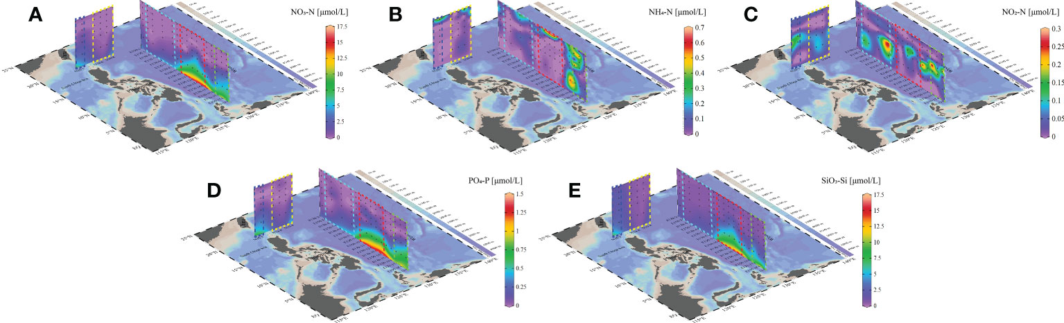
Figure 3 Inorganic Nutrients [NO₃-N (A), NH₄-N (B), NO₂-N (C), PO₄-P (D), SiO₃-Si (E)] distribution during the sample period in the WPO.

Distribution of diagnostic pigments and phytoplankton communities

According to the results of HPLC-CHEMTAX, the spatio-temporal variation of each phytoplankton and its diagnostic pigments exhibited similarity, with pigments primarily concentrated in the SCS mass and the junction of ME and HE mass, and distributed in 25-100 m range (Figure 4). Notably, Chl a (0-1.172 μg/L) and DV-Chl a (0-0.230 μg/L) were the most abundant and contributed them most of biomass of total pigments, while the abundance of Chl b (0-0.229 μg/L) was also higher than other pigments. This made Prochlorophytes (0-0.173 μg/L) one of the dominant phytoplankton in the WPO. Hex-Fuco (0-0.154 μg/L), Fuco (0-0.192 μg/L), and Pras (0-0.024 μg/L) were associated with Haptophytes (0-0.576 μg/L), Diatoms (0-0.252 μg/L), and Prasinophytes (0-0.130 μg/L), respectively, and were also dominant phytoplankton in the shallow layer of the WPO, primarily distributed in the 50-100 m layer.

FIGURE 4

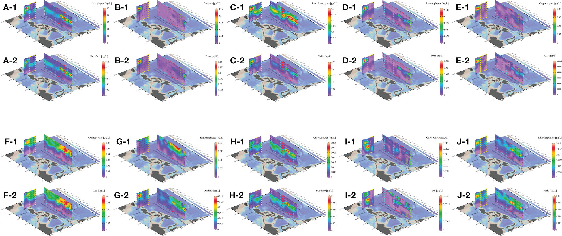
Figure 4 Phytoplankton communities and their marker pigment distributions during the sample period in the WPO. Haptophytes (A-1), Hex-Fuco (A-2), Diatoms (B-1), Fuco (B-2), Prochlorophytes (C-1), Chl b (C-2), Prasinophytes (D-1), Pras (D-2), Cryptophytes (E-1), Allo (E-2), Cyanbacteria (F-1), Zea (F-2), Euglenopytes (G-1), Diadino (G-2), Chrysophytes (H-1), But-Fuco (H-2), Chlorophytes (I-1), Lut (I-2), Dinoflagellates (J-1), Perid (J-2).

In the 130°E section, Haptophytes and Prasinophytes only found in the 0-10°N area, while Prochlorophytes were distributed throughout the 50-100 m layer. The high concentration area of Diatoms (0-0.252 μg/L) only appeared in 100 m of equatorial region, and another high concentration region was observed in the 20°N section, located in 50 m of the SCS mass. Allo (0-0.007 μg/L), Zea (0-0.102 μg/L), Diadino (0-0.017 μg/L), But-fuco (0-0.095 μg/L), Lut (0-0.004 μg/L), and Perid (0-0.014 μg/L) represented the concentration of Cryptophytes (0-0.097 μg/L), Cyanobacteria (0-0.068 μg/L), Chrysophytes (0-0.040 μg/L), Dinoflagellates (0-0.015 μg/L), Euglenophytes (0-0.021 μg/L), and Chlorophytes (0-0.033 μg/L), respectively (Figure 5). These were found to be lower than the aforementioned phytoplankton, with distinctive differences in distribution. Cyanobacteria was the dominant community in the surface of the WPO and gathered prominently in the junction of the HE and ME mass, while Euglenophytes were the second major community in the surface. The concentration of Chlorophytes was the lowest, and their distribution was dispersed with almost no continuous distribution. Other pigments, namely α-Car (0-0.039 μg/L) and β-Car (0-0.051 μg/L), exhibited distinct distribution in the study area. Specifically, α-Car was primarily distributed in the shallow layer, particularly in 0-100 m layer, while β-Car was more prevalent in the 100-200 m layer. Interestingly, the variation of these two carotene pigments displayed opposite variations, with α-Car being concentrated in the 100-200 m layer and β-Car in 0-100 m.

FIGURE 5

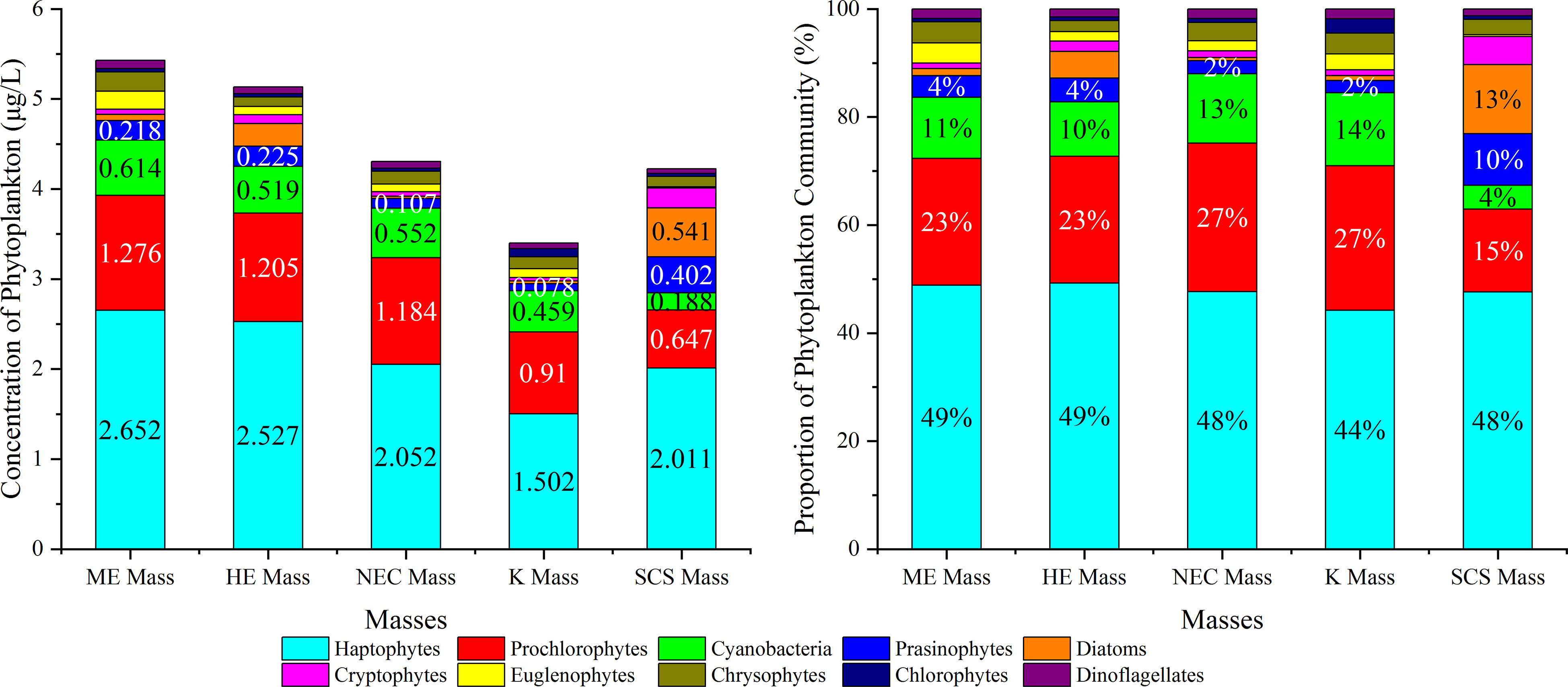
Figure 5 Concentrations (left) and Proportions (right) of phytoplankton community during the sample period in the WPO.

Haptophytes and Prochlorophytes were the primary contributors to the total biomass across all masses, with Cyanobacteria being the third most abundant phytoplankton biomass. However, in the SCS mass, Diatoms and Prochlorophytes accounted for almost the same proportion, and the abundance of Diatoms and Prasinophytes was higher than in other masses. Cryptophytes, Euglenophytes, Chrysophytes, Chlorophytes, and Dinoflagellates comprised less than 5% of the total phytoplankton biomass.

Size-fractionated phytoplankton

According to previous study, the concentrations and proportions of microphytoplankton, nanophytoplankton and picophytoplankton were calculated (Figure 6) (Uitz et al., 2006). The phytoplankton communities in the study area were dominated by nanophytoplankton (0-0.32 μg/L) and picophytoplankton (0-0.51 μg/L), with nanophytoplankton distributed in the 100-200 m layer and picophytoplankton contributing the most primary production in the 0-100 m layer. The contribution of microphytoplankton (0-0.52 μg/L) was negligible in most areas, except for the SCS and HE mass, where microphytoplankton concentration in the 25-100 m layer was slightly higher than in other regions. It is evident that, except in the SCS mass, nanophytoplankton and picophytoplankton accounted for 36.1-42.1% and 49.1-53.0%, respectively, while microphytoplankton only occupied 7.7-14.8%. In contrast, the proportion of microphytoplankton in the SCS mass rose to 22.3%, which was clearly different from in other masses.

FIGURE 6

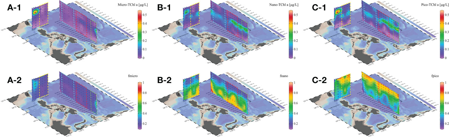
Figure 6 Size-fractionated concentrations [Micro-Chl a (A-1), Nano-Chl a (B-1), Pico-Chl a (C-1)] and proportion [f_micro (A-2), f_nano (B-2), f_pico (C-2)] of phytoplankton during the sample period in the WPO.

Discussion

Impacts of currents and eddies in the WPO

Marine dynamics can have a significant impact the phytoplankton community composition and spatio-temporal variability. Conversely, the distribution characteristics of phytoplankton can reflect spatio-temporal variability in the marine ecosystem. The diagnostic pigments of phytoplankton can clarify their community compositions and regulate their response to environmental factors. Estuarine-coastal waters are generally nutrient-rich, with DIN, phosphate, silicate of 10.4 μmol/L, 0.38 μmol/L, and 14.7 μmol/L (Carstensen et al., 2015), respectively, which were higher than those in the 75m-100m layer of our survey area. Our study results indicate that the WPO is a classical oligotrophic ocean that may be affected by complex hydrological and chemical conditions. The distribution of phytoplankton was found to be limited in several zones, which was obviously related to nutrient concentration. This lack of nutrients in the euphotic zone directly restricted the biomass and distribution of phytoplankton.

According to previous studies, the survey area was influenced by a north equatorial current system (Lukas et al., 1997; Xie et al., 2009). During the sampling period, hydrological conditions were similar to those in spring, with light intensity and temperature were suitable for phytoplankton. A relative high upwelling of nutrients in study area was observed, which was consistent with high phytoplankton biomass. Notably, the concentration of phytoplankton was particularly high in the junction area between HE and ME mass, specifically between E130-12 and E130-19 station, which differed from other stations (Figure 7). The advection flow and upwelling caused by HE and ME were likely responsible for this phenomenon, as they enabled the phytoplankton in the upper layer of water to uptake more nutrient and have more time for photosynthesis. The interaction of HE and ME led to the formation of baroclinic field that brought cold hypohaline intermediate layer water with relatively high nutrients into surface layer (Messié and Radenac, 2006). As there was an upwelling water mass phenomenon in the junction area between HE and ME mass caused by the divergence interaction, it extracted deeper seawater with high nutrient concentrations into the surface layer.

FIGURE 7

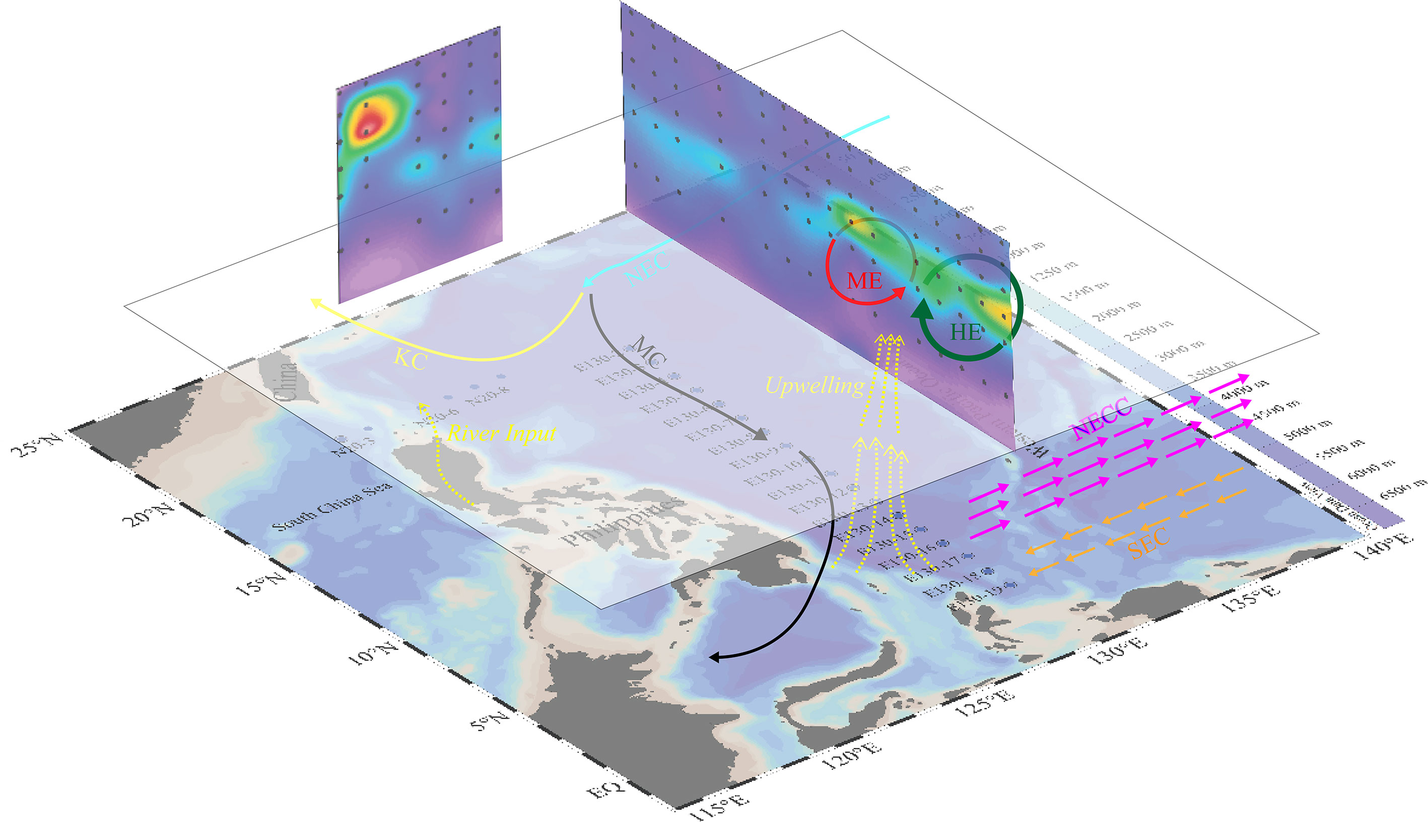
Figure 7 Currents and eddies impacts on phytoplankton communities during the sample period in the WPO. (Light blue arrows represent NEC, purple arrows represent NECC, yellow arrows represent KC, and black arrows represent MC. Red cycle represents ME and green cycle represents HE).

The gathering of phytoplankton in the SCS mass may be caused by the KC, but there was no eddy to interact with the KC. In this case, the offshore flow could scour materials from lands, and caused upwelling in the SCS mass area (Ranthodsang et al., 2020; Li et al., 2021). NH₄-N in seawater is typically produced by the degradation of phytoplankton organisms. In junction of ME and HE mass, NH₄-N was widely distributed from the surface to deeper seawater layer. However, in the SCS mass, NH₄-N was only distributed in the surface layer, with lower concentrations of other nutrients than in the ME and HE mass. Nevertheless, the biomass of phytoplankton communities suggested that there must have been sufficient nutrients input to sustain this biomass. Another nutrients source was rivers runoff (Amaya et al., 2012). The rivers runoff and KC offshore flow would have been assimilated by phytoplankton before settlement happened, affording high biomass of phytoplankton communities.

Controlling factors of the temporal and spatial distribution of phytoplankton communities

The RDA ordination analysis of phytoplankton community dataset identifies temperature, salinity, NH₄-N, NO₃-N, NO₂-N, PO₄-P, SiO₃-Si, DIN, N/P, and DIN/DSi as subset of environmental variables that explain significant and independent amounts of variation. Basically, the result reveals that NO₃-N, PO₄-P, SiO₃-Si, DIN, DIN/DSi were primary nutrient variables in all masses. The RDA analysis indicates that NO₃-N, PO₄-P, SiO₃-Si, DIN, DIN/DSi, and salinity were negatively correlated with temperature and NH₄-N, whereas NO₂-N and N/P were not strongly related to other environmental variables.

The RDA analysis of the phytoplankton community dataset in the SCS mass identified NO₃-N, SiO₃-Si, PO₄-P, and salinity as strongly correlated variables, while negatively correlated to temperature and NH₄-N. However, NO₂-N was weakly correlated with other environmental variables. The correlation between environmental variables and phytoplankton communities in the SCS mass was weak, with only Cryptophytes and Chlorophytes showing a positive correlation with temperature (Figure 8A). In turn, temperature, NO₃-N, PO₄-P, and DIN were largely associated with phytoplankton communities. In the KC (Figure 8B) and the ME mass (Figure 8D), Haptophytes showed a strong positive correlation with NO₃-N, PO₄-P, and DIN, while being negatively correlated with temperature. Cryptophytes, Dinoflagellates and Euglenophytes were weakly correlated with other variables in the KC mass. Prasinophytes, Chlorophytes, and Chrysophytes were positively correlated with salinity and NO₂-N. In the NEC mass (Figure 8C), Prochlorophytes and Cyanobacteria were positively correlated with these nutrients, but negatively correlated with temperature. On the other hand, Chlorophytes was positively correlated with NO₃-N, PO₄-P, and DIN. Notably, the axis 1 in ME mass accounted for 73.09% of the variance. Therefore, it can be concluded that Cyanobacteria, Euglenophytes, Dinoflagellates were positively correlated with temperature, but negatively correlated with NO₃-N, PO₄-P, and DIN, while Haptophytes, Chrysophytes, and Prasinophytes were strongly positively correlated with NO₃-N, PO₄-P, and DIN. In the HE mass (Figure 8E), Chrysophytes, Haptophytes, and Prasinophytes were strongly positively correlated with NO₃-N, PO₄-P, DIN, and salinity, while being negatively with temperature and NH₄-N. In turn, the correlation of Cyanobacteria, Dinoflagellates, Euglenophytes and Prochlorophytes was opposite. Combined with the impacts of currents and eddies, it can be inferred that the main contributors of phytoplankton communities in the ME and HE mass were related to nutrients, while this correlation was weaker in the NEC and KC mass. In the SCS mass, the distribution of phytoplankton communities was weakly correlated to environmental factors.

FIGURE 8

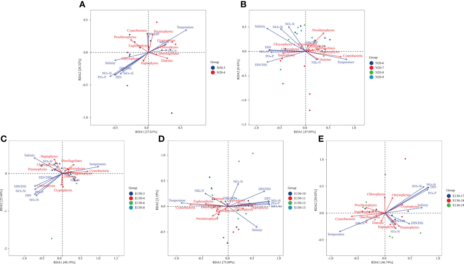
Figure 8 Redundancy analysis of phytoplankton communities and environmental parameters during the sample period in the WPO [SCS mass (A), KC mass (B), NEC mass (C), ME mass (D), HE mass (E)].

Based on the RDA of variant trend and phytoplankton biomass, it can be concluded that hydrological factors had little impact on limiting the distribution and biomass of phytoplankton in the KC and NEC mass, where nutrients only played a minor role. In the HE and HE mass, however, hydrological factors, particularly PO₄-P and NO₃-N, significantly determined the biomass and distribution of phytoplankton communities. Combined with the currents and eddies conditions during the sample period, it appears that the primary influence factor causing the invasion of rich-nutrient upwelling into the euphotic layer is located at the junction between HE and ME mass, as demonstrated by the divergence. The redundancy analysis shows a significant trend that the primary phytoplankton communities in the SCS mass were still related to nutrients. Additionally, the biomass of phytoplankton communities was even higher than KC mass and similar to NEC mass, indicating that hydrological factors, especially nutrient conditions, can support high phytoplankton biomass in the SCS mass. Moreover, the biomass of microphytoplankton in the SCS mass was considerably higher than in other masses, with Diatoms and Prasinophytes having a higher proportion.

Based on the correlation analysis of phytoplankton communities and environmental parameters (Figure 9), a high relationship was observed between the abundance of Haptophytes and Prochlorophytes in the ME and HE mass, as previously mentioned. However, the abundance of Haptophytes and Prochlorophytes in the SCS mass differs significantly from that in other masses, possibly due to offshore flow caused by KC (Holbrook et al., 2021), which could provide nutrients to support the reproduction of phytoplankton communities. Furthermore, the intrusion current from South China Sea may be another source to provide nutrients.

FIGURE 9

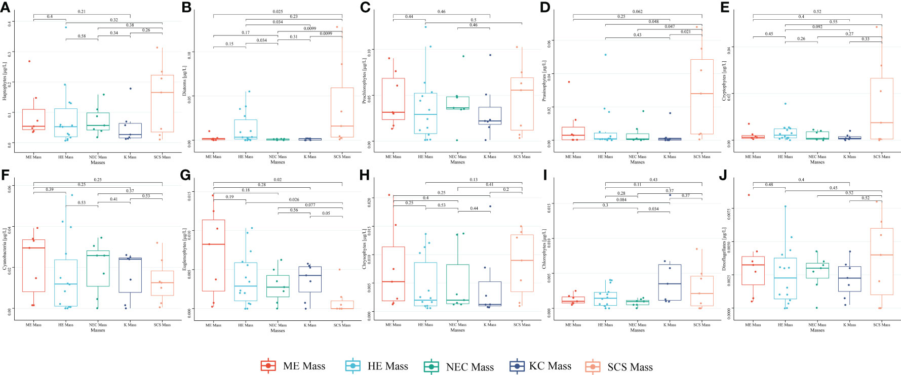
Figure 9 Variance analysis of phytoplankton biomass in the different water masses. [Haptophytes (A), Diatoms (B), Prochlorophytes (C), Prasinophytes (D), Cryptophytes (E), Cyanbacteria (F), Euglenopytes (G), Chrysophytes (H), Chlorophytes (I), Dinoflagellates (J)].

Influences of biochemical processes of phytoplankton

The correlation analysis between phytoplankton communities and sized-fractionated phytoplankton provides additional evidence to support the above-mentioned assumptions (Figure 6). The KC and SCS mass are evidently influenced by hydrological environment conditions of The Kuroshio, which is a part of the western boundary current (Nishibe et al., 2017). The spatial distribution of the phytoplankton communities is affected by the intrusion of the southern water into the north (Yamamoto and Nishizawa, 1986), which transported eutrophic deep water mass into surface as a warm filament. This indicates that picophytoplankton and nanophytoplankton were major contributors to the total phytoplankton biomass. Combining the distribution of phytoplankton communities, the dominant populations were Haptophytes, Diatoms, and Prochlorophytes (Figure 9). Considering the biomass of phytoplankton, it is hard to ignore the diversity of phytoplankton communities in each mass. The biomass of Prasinophytes, Euglenophytes, and Cryptophytes in the SCS mass differs significantly from in other masses, with the abundance of other communities being much lower than these three species.

Previous studies have shown that the nutrient structure significantly affects the phytoplankton community structure (Justić et al., 1995), with N/P and DIN/DSi ratios being the major limiting factors (Brauer et al., 2012). Nitrogen limitation is common in open ocean, but the average N/P ratios in SCS (16.43/1) and KC mass (17.22/1) were very close to the Redfield ratio (16/1), indicating weaker nitrogen limitation in the SCS and KC mass than in the other masses. The N/P ratios at the 0-100 m layer showed obvious difference, especially in HE, ME, and KC mass. On the other hand, DIN/DSi ratios in NEC, KC, and ME mass had a distinctive distribution at the depth shallower than 100 m. Furthermore, low DIN/DSi ratios in different masses apparently caused the blooming of Diatoms (Sarthou et al., 2005). Nano-Diatoms and Pico-Diatoms, with higher surface-to-volume ratios, have more efficient exploitation of low nutrient concentrations, allowing them to stay in subsurface layer. Because of the divergence and the cell characteristics of phytoplankton, the rates of nutrient absorption by phytoplankton with various size are different (Lukas, 2001; Zhang et al., 2019a). The size of microphytoplankton is relatively large, so its biomass is relatively high in high nutrient water. Nanophytoplankton and picophytoplankton have a relatively smaller size, but their surface-to-volume are higher than microphytoplankton (Leruste et al., 2019). Therefore, in low nutrient water, the biomass of nanophytoplankton and picophytoplankton is relatively high. However, even with the occurrence of divergence phenomenon, the total concentration of nutrient in the WPO still is low (Anjusha et al., 2018), with the biomass of microphytoplankton with relatively low nutrient absorption rate was correspondingly low (Behrenfeld et al., 2015). Meanwhile, micro-Diatoms have relatively low surface-to-volume ratios and require nutrient-rich conditions for growth, causing them sink to deeper layer for nutrient absorption and rise to upper euphotic zone for photosynthesis (Armbrust, 2009). However, even though micro-Diatoms can sink and rise, the nutrients concentration in the sub-intermediate layer water is still not rich enough. This caused the biomass of phytoplankton in the SCS mass was higher than in other area but still lower than picophytoplankton and nanophytoplankton. In the meantime, even though the absorption rate of picophytoplankton is higher than other two phytoplankton species, its biomass is still limited by the size of cell. While with relatively high absorption rates and more monomer biomass, nanophytoplankton became the major contributor to the total phytoplankton biomass (Noman et al., 2019). Furthermore, other eddies can also affect the distribution of phytoplankton (Dickey et al., 1998). Cold-core eddies upwell the nutrients to the euphotic zone through eddy-driven upwelling and enhance Chl a production, while warm-core eddies suppress the availability of nutrients in the euphotic zone and reduce Chl a production by pushing the nutracline downwards via eddy-driven downwelling (Vidya and Kurian, 2018).

In summary, this study confirms previous findings on distribution characteristics of phytoplankton communities and provides new information regarding the environmental and biological regulations of phytoplankton communities in the WPO. The study finds that Haptophytes, Prochlorophytes and Cyanobacteria were the primary contributors to total biomass. The nutrients, especially NO₃-N and PO₄-P, were identified as the major controlling variables for the biomass and distribution of primary phytoplankton communities. Furthermore, the study finds a negative correlation between temperature and primary phytoplankton communities. In the 130°E section, the interaction of HE and ME mass caused the divergence during the sample period in the WPO, which brought relatively eutrophic deep seawater into the euphotic layer. This explains why there was a high biomass of phytoplankton communities gathering in the junction area of HE and ME mass. The study also finds that picophytoplankton and nanophytoplankton were the main size-fractionated phytoplankton in this section. In the 20°N section, the study identifies KC invasion and KC offshore as primary factors causing a relatively high biomass of phytoplankton. Additionally, the study also finds that micro-Diatoms had a higher proportion in this section due to their relatively low surface-to-volume ratios, ability to sink to deeper layer for nutrient absorption and rise to upper euphotic layer for photosynthesis.

Data availability statement

The raw data supporting the conclusions of this article will be made available by the authors, without undue reservation.

Author contributions

GZ: Investigation, Data curation, Writing-review and editing, Funding acquisition. ZL: Writing-original draft, Data analysis. ZZ: Investigation. CD: Sample analysis. JS: Conceptualization, Methodology, Project administration, Resources, Supervision, Visualization, Review and editing. All authors contributed to the article and approved the submitted version.

Funding

This research was supported by the National Natural Science Foundation of China (Nos. 42106095, 41876134, 41676112, and 41276124) and the Changjiang Scholar Program of Chinese Ministry of Education (No. T2014253). Data acquisition and sample collections were supported by NSFC Open Research Cruise (No. NORC2016-09), funded by Shiptime Sharing Project of the NSFC. This cruise was conducted onboard R/V KEXUE by the Institute of Oceanography, Chinese Academy of Sciences, China.

Acknowledgments

We wish to thank Prof. Hui Zhou as cruise Chief Scientist, the captains and crew of R/V KEXUE, all scientists and technicians who helped with sample collection and CTD data during the cruise. GZ was also supported by the postdoc fellowship from Tianjin University of Science and Technology.

Conflict of interest

The authors declare that the research was conducted in the absence of any commercial or financial relationships that could be construed as a potential conflict of interest.

Publisher’s note

All claims expressed in this article are solely those of the authors and do not necessarily represent those of their affiliated organizations, or those of the publisher, the editors and the reviewers. Any product that may be evaluated in this article, or claim that may be made by its manufacturer, is not guaranteed or endorsed by the publisher.

References

Amaya F. L., Gonzales T. A., Hernandez E. C., Luzano E. V., Mercado N. P. (2012). Estimating point and non-point sources of pollution in biñan river basin, the Philippines. APCBEE Proc. 1, 233–238. doi: 10.1016/j.apcbee.2012.03.038

CrossRef Full Text | Google Scholar

An B., Li T., Liu J., Sun H., Chang F. (2018). Spatial distribution and controlling factors of planktonic foraminifera in the modern western pacific. Quaternary Int. 468, 14–23. doi: 10.1016/j.quaint.2018.01.003

CrossRef Full Text | Google Scholar

Anjusha A., Jyothibabu R., Jagadeesan L., Savitha K. M. M., Albin K. J. (2018). Seasonal variation of phytoplankton growth and microzooplankton grazing in a tropical coastal water (off kochi), southwest coast of India. Continental Shelf Res. 171, 12–20. doi: 10.1016/j.csr.2018.10.009

CrossRef Full Text | Google Scholar

Armbrust E. V. (2009). The life of diatoms in the world's oceans. Nature 459, 185. doi: 10.1038/nature08057

PubMed Abstract | CrossRef Full Text | Google Scholar

Behrenfeld M. J., O’Malley R. T., Boss E. S., Westberry T. K., Graff J. R., Halsey K. H., et al. (2015). Revaluating ocean warming impacts on global phytoplankton. Nat. Climate Change 6 (3), 323–330. doi: 10.1038/nclimate2838

CrossRef Full Text | Google Scholar

Behrens M. K., Pahnke K., Schnetger B., Brumsack H.-J. (2018). Sources and processes affecting the distribution of dissolved Nd isotopes and concentrations in the West pacific. Geochimica Cosmochimica Acta 222, 508–534. doi: 10.1016/j.gca.2017.11.008

CrossRef Full Text | Google Scholar

Brauer V. S., Stomp M., Huisman J. (2012). The nutrient-load hypothesis: patterns of resource limitation and community structure driven by competition for nutrients and light. Am. Nat. 179 (6), 721–740. doi: 10.1086/665650

PubMed Abstract | CrossRef Full Text | Google Scholar

Carstensen J., Klais R., Cloern J. E. (2015). Phytoplankton blooms in estuarine and coastal waters: seasonal patterns and key species. Estuarine Coast. Shelf Sci. 162, 98–109. doi: 10.1016/j.ecss.2015.05.005

CrossRef Full Text | Google Scholar

Collins M., An S.-I., Cai W., Ganachaud A., Guilyardi E., Jin F.-F., et al. (2010). The impact of global warming on the tropical pacific ocean and El niño. Nat. Geosci. 3 (6), 391–397. doi: 10.1038/ngeo868

CrossRef Full Text | Google Scholar

Dickey T., Marra J., Sigurdson D. E., Weller R. A., Kinkade C. S., Zedler S. E., et al. (1998). Seasonal variability of bio-optical and physical properties in the Arabian Sea: October 1994–October 1995. Deep Sea Res. Part II: Topical Stud. Oceanography 45 (10), 2001–2025. doi: 10.1016/S0967-0645(98)00061-7

CrossRef Full Text | Google Scholar

Field C. B., Behrenfeld M. J., Randerson J. T., Falkowski P. (1998). Primary production of the biosphere: integrating terrestrial and oceanic components. Science 281 (5374), 237–240. doi: 10.1126/science.281.5374.237

PubMed Abstract | CrossRef Full Text | Google Scholar

Grasshoff K., Kremling K., Ehrhardt M. (2009). Methods of seawater analysis (John Wiley & Sons).

Google Scholar

Higgins H. W., W S., Schluter L. (2011). Quantitative interpretation of chemotaxonomic pigment data. Chemotaxonomy Appl. Oceanography Phytoplankton Pigments: Characterization, 257–313. doi: 10.1017/CBO9780511732263.010

CrossRef Full Text | Google Scholar

Holbrook N. J., Hernaman V., Koshiba S., Lako J., Kajtar J. B., Amosa P., et al. (2021). Impacts of marine heatwaves on tropical western and central pacific island nations and their communities. Global Planetary Change 103680, 299–308. doi: 10.1016/j.gloplacha.2021.103680

CrossRef Full Text | Google Scholar

Hong L., Zhou Y., Zhang D., Du M., Wang Y., Wang C. (2014). The distribution of chlorophyll a in the eastern equatorial pacific ocean in boreal autumn. Acta Ecologica Sin. 34 (3), 154–159. doi: 10.1016/j.chnaes.2014.03.004

CrossRef Full Text | Google Scholar

Hu D., Wu L., Cai W., Gupta A. S., Ganachaud A., Qiu B., et al. (2015). Pacific western boundary currents and their roles in climate. Nature 522 (7556), 299–308. doi: 10.1038/nature14504

PubMed Abstract | CrossRef Full Text | Google Scholar

Hyun M. J., Won J., Choi D. H., Lee H., Lee Y., Lee C. M., et al. (2022). A CHEMTAX study based on picoeukaryotic phytoplankton pigments and next-generation sequencing data from the Ulleungdo–Dokdo marine system of the East Sea (Japan sea): improvement of long-unresolved underdetermined bias. J. Mar. Sci. Eng. 10 (12), 1967. doi: 10.3390/jmse10121967

CrossRef Full Text | Google Scholar

Jia Q., Li T., Xiong Z., Steinke S., Jiang F., Chang F., et al. (2018). Hydrological variability in the western tropical pacific over the past 700kyr and its linkage to northern hemisphere climatic change. Palaeogeography Palaeoclimatology Palaeoecol. 493, 44–54. doi: 10.1016/j.palaeo.2017.12.039

CrossRef Full Text | Google Scholar

Justić D., Rabalais N. N., Turner R. E. (1995). Stoichiometric nutrient balance and origin of coastal eutrophication. Mar. Pollut. Bull. 30 (1), 41–46. doi: 10.1016/0025-326X(94)00105-I

CrossRef Full Text | Google Scholar

Leruste A., Pasqualini V., Garrido M., Malet N., De Wit R., Bec B. (2019). Physiological and behavioral responses of phytoplankton communities to nutrient availability in a disturbed Mediterranean coastal lagoon. Estuarine Coast. Shelf Sci. 219, 176–188. doi: 10.1016/j.ecss.2019.02.014

CrossRef Full Text | Google Scholar

Li X.-Y., Yu R.-C., Geng H.-X., Li Y.-F. (2021). Increasing dominance of dinoflagellate red tides in the coastal waters of yellow Sea, China. Mar. pollut. Bull. 168, 112439. doi: 10.1016/j.marpolbul.2021.112439

PubMed Abstract | CrossRef Full Text | Google Scholar

Lin M., Wang C., Wang Y., Xiang P., Wang Y., Lian G., et al. (2011). Zooplanktonic diversity in the western pacific. Biodiversity Sci. 19 (6), 646. doi: 10.3724/SP.J.1003.2011.09178

CrossRef Full Text | Google Scholar

Liu S.-S., Yang G.-P., He Z., Gao X.-X., Xu F. (2021b). Oceanic emissions of methyl halides and effect of nutrients concentration on their production: a case of the western pacific ocean (2°N to 24°N). Sci. Total Environ. 769, 144488. doi: 10.1016/j.scitotenv.2020.144488

PubMed Abstract | CrossRef Full Text | Google Scholar

Liu Q., Zhao Q., Jiang Y., Li Y., Zhang C., Li X., et al. (2021a). Diversity and co-occurrence networks of picoeukaryotes as a tool for indicating underlying environmental heterogeneity in the Western pacific ocean. Mar. Environ. Res. 170, 105376. doi: 10.1016/j.marenvres.2021.105376

PubMed Abstract | CrossRef Full Text | Google Scholar

Lukas R. (2001). “Pacific ocean equatorial currents,” in Encyclopedia of ocean sciences, 3rd ed. Eds. Cochran J. K., Bokuniewicz H. J., Yager P. L. (Oxford: Academic Press), 429–436.

Google Scholar

Lukas R., Yamagata T., McCreary J. P. (1997). Pacific low-latitude western boundary currents and the Indonesian throughflow. Oceanographic Literature Rev. 44 (1), 4. doi: 10.1029/96JC01204

CrossRef Full Text | Google Scholar

Ma J., Song J., Li X., Wang Q., Sun X., Zhang W., et al. (2021). Seawater stratification vs. plankton for oligotrophic mechanism: a case study of M4 seamount area in the Western pacific ocean. Mar. Environ. Res. 169, 105400. doi: 10.1016/j.marenvres.2021.105400

PubMed Abstract | CrossRef Full Text | Google Scholar

Mackey D. J., Higgins H. W., Mackey M. D., Holdsworth D. (1998). Algal class abundances in the western equatorial pacific: estimation from HPLC measurements of chloroplast pigments using CHEMTAX. Deep Sea Res. Part I Oceanographic Res. Papers 45 (9), 1441–1468. doi: 10.1016/S0967-0637(98)00025-9

CrossRef Full Text | Google Scholar

Mackey M. D., Mackey D. J., Higgins H. W., Wright S. W. (1996). CHEMTAX - a program for estimating class abundances from chemical markers: application to HPLC measurements of phytoplankton. Mar. Ecol. Prog. Ser. 144, 265–283. doi: 10.3354/meps144265

CrossRef Full Text | Google Scholar

Masumoto Y., Yamagata T. (1991). Response of the Western tropical pacific to the Asian winter monsoon: the generation of the Mindanao dome. J. Phys. Oceanography 21 (9), 1386–1398. doi: 10.1175/1520-0485(1991)021<1386:Rotwtp>2.0.Co;2

CrossRef Full Text | Google Scholar

Messié M., Radenac M.-H. (2006). Seasonal variability of the surface chlorophyll in the western tropical pacific from SeaWiFS data. Deep Sea Res. Part I: Oceanographic Res. Papers 53 (10), 1581–1600. doi: 10.1016/j.dsr.2006.06.007

CrossRef Full Text | Google Scholar

Mori Y., Nishioka J., Fujio S., Yamashita Y. (2021). Transport of dissolved black carbon from marginal sea sediments to the western north pacific. Prog. Oceanography 193, 102552. doi: 10.1016/j.pocean.2021.102552

CrossRef Full Text | Google Scholar

Nishibe Y., Takahashi K., Sato M., Kodama T., Kakehi S., Saito H., et al. (2017). Phytoplankton community structure, as derived from pigment signatures, in the kuroshio extension and adjacent regions in winter and spring. J. Oceanography 73 (4), 463–478. doi: 10.1007/s10872-017-0415-3

CrossRef Full Text | Google Scholar

Nomaki H., Rastelli E., Alves A., Suga H., Ramos S., Kitahashi T., et al. (2021). Abyssal fauna, benthic microbes, and organic matter quality across a range of trophic conditions in the western pacific ocean. Prog. Oceanography 195, 102591. doi: 10.1016/j.pocean.2021.102591

CrossRef Full Text | Google Scholar

Noman M. A., Sun J., Gang Q., Guo C., Islam M. S., Li S., et al. (2019). Factors regulating the phytoplankton and tintinnid microzooplankton communities in the East China Sea. Continental Shelf Res. 181, 14–24. doi: 10.1016/j.csr.2019.05.007

CrossRef Full Text | Google Scholar

Paul M., Nikathithara Velappan M., Nanappan U., Gopinath V., Thekkendavida Velloth R., Rajendran A., et al. (2021). Characterization of phytoplankton size-structure based productivity, pigment complexes (HPLC/CHEMTAX) and species composition in the Cochin estuary (southwest coast of india): special emphasis on diatoms. Oceanologia 63, 463–481. doi: 10.1016/j.oceano.2021.05.004

CrossRef Full Text | Google Scholar

Ranthodsang M., Waewsak J., Kongruang C., Gagnon Y. (2020). Offshore wind power assessment on the western coast of Thailand. Energy Rep. 6, 1135–1146. doi: 10.1016/j.egyr.2020.04.036

CrossRef Full Text | Google Scholar

Sarthou G., Timmermans K. R., Blain S., Tréguer P. (2005). Growth physiology and fate of diatoms in the ocean: a review. J. Sea Res. 53 (1), 25–42. doi: 10.1016/j.seares.2004.01.007

CrossRef Full Text | Google Scholar

Schlitzer R. (2002). Interactive analysis and visualization of geoscience data with ocean data view. Comput. Geosciences 28 (10), 1211–1218. doi: 10.1016/S0098-3004(02)00040-7

CrossRef Full Text | Google Scholar

Schlüter L., Henriksen P., Nielsen T. G., Jakobsen H. H. (2011). Phytoplankton composition and biomass across the southern Indian ocean. Deep Sea Res. Part I: Oceanographic Res. Papers 58 (5), 546–556. doi: 10.1016/j.dsr.2011.02.007

CrossRef Full Text | Google Scholar

Song Y., Guo Y., Liu H., Zhang G., Zhang X., Thangaraj S., et al. (2022). Water quality shifts the dominant phytoplankton group from diatoms to dinoflagellates in the coastal ecosystem of the bohai bay. Mar. Pollut. Bull. 183, 114078. doi: 10.1016/j.marpolbul.2022.114078

PubMed Abstract | CrossRef Full Text | Google Scholar

Suzuki T., Sakamoto T. T., Nishimura T., Okada N., Emori S., Oka A., et al. (2005). Seasonal cycle of the Mindanao dome in the CCSR/NIES/FRCGC atmosphere-ocean coupled model. Geophysical Res. Lett. 32 (17), 1–4. doi: 10.1029/2005GL023666

CrossRef Full Text | Google Scholar

Swan C. M., Vogt M., Gruber N., Laufkoetter C. (2016). A global seasonal surface ocean climatology of phytoplankton types based on CHEMTAX analysis of HPLC pigments. Deep Sea Res. Part I: Oceanographic Res. Papers 109, 137–156. doi: 10.1016/j.dsr.2015.12.002

CrossRef Full Text | Google Scholar

Turk-Kubo K. A., Connell P., Caron D., Hogan M. E., Farnelid H. M., Zehr J. P. (2018). In situ diazotroph population dynamics under different resource ratios in the north pacific subtropical gyre. Front. Microbiol. 9. doi: 10.3389/fmicb.2018.01616

CrossRef Full Text | Google Scholar

Uitz J., Claustre H., Morel A., Hooker S. B. (2006). Vertical distribution of phytoplankton communities in open ocean: an assessment based on surface chlorophyll. J. Geophysical Research: Oceans 111 (C8), 1–23. doi: 10.1029/2005JC003207

CrossRef Full Text | Google Scholar

Vidya P. J., Kurian S. (2018). Impact of 2015-2016 ENSO on the winter bloom and associated phytoplankton community shift in the northeastern Arabian Sea. J. Mar. Syst. 186, 96–104. doi: 10.1016/j.jmarsys.2018.06.005

CrossRef Full Text | Google Scholar

Waga H., Fujiwara A., Hirawake T., Suzuki K., Yoshida K., Abe H., et al. (2022). Primary productivity and phytoplankton community structure in surface waters of the western subarctic pacific and the Bering Sea during summer with reference to bloom stages. Prog. Oceanography 201, 102738. doi: 10.1016/j.pocean.2021.102738

CrossRef Full Text | Google Scholar

Wang J.-X., Kong F.-Z., Geng H.-X., Zhang Q.-C., Yuan Y.-Q., Yu R.-C. (2021). CHEMTAX analysis of phytoplankton assemblages revealed potential indicators for blooms of haptophyte phaeocystis globosa. Ecol. Indic. 131, 108177. doi: 10.1016/j.ecolind.2021.108177

CrossRef Full Text | Google Scholar

Wright S. W., Jeffrey S. W. (2006). “Pigment markers for phytoplankton production,” in Marine organic matter: biomarkers, isotopes and DNA. Ed. Volkman J. K. (Berlin, Heidelberg: Springer Berlin Heidelberg), 71–104.

Google Scholar

Wright S. W., van den Enden R. L., Pearce I., Davidson A. T., Scott F. J., Westwood K. J. (2010). Phytoplankton community structure and stocks in the southern ocean (30–80°E) determined by CHEMTAX analysis of HPLC pigment signatures. Deep Sea Res. Part II: Topical Stud. Oceanography 57 (9), 758–778. doi: 10.1016/j.dsr2.2009.06.015

CrossRef Full Text | Google Scholar

Xie S.-P., Hu K., Hafner J., Tokinaga H., Du Y., Huang G., et al. (2009). Indian Ocean capacitor effect on indo–Western pacific climate during the summer following El niño. J. Climate 22 (3), 730–747. doi: 10.1175/2008jcli2544.1

CrossRef Full Text | Google Scholar

Yamamoto T., Nishizawa S. (1986). Small-scale zooplankton aggregations at the front of a kuroshio warm-core ring. Deep Sea Res. Part A. Oceanographic Res. Papers 33 (11), 1729–1740. doi: 10.1016/0198-0149(86)90076-2

CrossRef Full Text | Google Scholar

Yuan D., Wang J., Xu T., Xu P., Hui Z., Zhao X., et al. (2011). Forcing of the Indian ocean dipole on the interannual variations of the tropical pacific ocean: roles of the Indonesian throughflow. J. Climate 24 (14), 3593–3608. doi: 10.1175/2011jcli3649.1

CrossRef Full Text | Google Scholar

Zhang D., Jian S., Sun J., Leng X., Zhang G. (2019b). Spatial-temporal dynamics of biogenic silica in the southern yellow Sea. Acta Oceanologica Sin. 38 (12), 101–110. doi: 10.1007/s13131-019-1516-1

CrossRef Full Text | Google Scholar

Zhang D., Wang C., Liu Z., Xu X., Wang X., Zhou Y. (2012). Spatial and temporal variability and size fractionation of chlorophyll a in the tropical and subtropical pacific ocean. Acta Oceanologica Sin. 31 (3), 120–131. doi: 10.1007/s13131-012-0212-1

CrossRef Full Text | Google Scholar

Zhang C., Yao X., Chen Y., Chu Q., Yu Y., Shi J., et al. (2019a). Variations in the phytoplankton community due to dust additions in eutrophication, LNLC and HNLC oceanic zones. Sci. Total Environ. 669, 282–293. doi: 10.1016/j.scitotenv.2019.02.068

PubMed Abstract | CrossRef Full Text | Google Scholar