 Kangkang Jin
 Jian Xu
 Xuefeng Zhang
94% of researchers rate our articles as excellent or good
Learn more about the work of our research integrity team to safeguard the quality of each article we publish.
Find out more
ORIGINAL RESEARCH article
Front. Mar. Sci. , 01 August 2023
Sec. Ocean Observation
Volume 10 - 2023 | https://doi.org/10.3389/fmars.2023.1182653
This article is part of the Research Topic Deep Learning for Marine Science View all 40 articles
Acoustic tracking of whales’ underwater cruises is essential for protecting marine ecosystems. For cetacean conservationists, fewer hydrophones will provide more convenience in capturing high-mobility whale positions. Currently, it has been possible to use two hydrophones individually to accomplish direction finding or ranging. However, traditional methods only aim at estimating one of the spatial parameters and are susceptible to the detrimental effects of reverberation superimposition. To achieve complete whale tracking under reverberant interference, in this study, an intelligent acoustic tracking model (CIAT) is proposed, which allows both horizontal direction discrimination and distance/depth perception by mining unpredictable features of position information directly from the received signals of two hydrophones. Specifically, the horizontal direction is discriminated by an enhanced cross-spectral analysis to make full use of the exact frequency of received signals and eliminate the interference of non-source signals, and the distance/depth direction combines convolutional neural network (CNN) with transfer learning to address the adverse effects caused by unavoidable acoustic reflections and reverberation superposition. Experiments with real recordings show that 0.13 km/MAE is achieved within 8 km. Our work not only provides satisfactory prediction performance, but also effectively avoids the reverberation effect of long-distance signal propagation, opening up a new avenue for underwater target tracking.
Whales play an extremely important role in the structure and dynamics of natural ecosystems (Roman et al., 2014). They can not only improve primary productivity (Henley et al., 2020), but also regulate carbon dioxide in the atmosphere and marine environment (Roman et al., 2016). Since the moratorium on commercial whaling in 1986, the global whale population has continued grown, with a concomitant increase in the frequency of the whale stranding (Parsons and Rose, 2022), which has attracted widespread attention. In 2020, Klaus pointed out the whale stranding typically occur during their migrations (Vanselow, 2020). Despite several attempts by some scholars to use satellite tags for individual movement behaviors, they still are unable to understand whale movements below the surface, which leaves the potential patterns or causes of whale stranding incompletely expressed (Perez et al., 2022). Therefore, mastering the continuous and high-precision movement trajectories of whales is of great value for the protection of whale diversity and stranding management.
Passive acoustic monitoring (PAM) offers a novel, long-term, large-scale monitoring advantage that can provide species distribution and activity information for vocal species, making it an ideal bioacoustic tool for whale tracking (Davis et al., 2017; Aulich et al., 2019). PAM utilizes a distributed single-receiver hydrophone system, which enables the estimation of cetacean population densities without the need for tracking and directly protecting whales during migration. Currently, there is a growing expectation for tracking systems designed for high-mobility whales to have a smaller design, low power consumption, and fewer hydrophones (Ferreira et al., 2021; Frasier et al., 2021; Cheeseman et al., 2022; Jones et al., 2022). Previous studies have explored the use of two hydrophones to determine the orientation or distance of underwater targets using acoustic-based technology. However, due to the coupling between the azimuth and distance parameters (Ding et al., 2020), the distance estimates expressed according to the analytic equations are poor when the azimuth varies with the interference of reverberation and acoustic reflections, which significantly reduces the tracking accuracy of the whales.
With the increasing development of artificial intelligence, new statistical prediction methods based on deep learning have shown better performance in existing underwater target location prediction. In recent years, more and more deep neural networks have been proposed one after another, such as CNNs (Song, 2018; White et al., 2022), deep neural networks (DNNs) (Yangzhou et al., 2019), recurrent neural networks (RNNs) (Shankar et al., 2020) and transformers (Kujawski and Sarradj, 2022). These models have been successfully applied in many fields of geophysics. Jiang et al. (2020) proposed a new algorithm fusing deep neural network and CNN for sound source orientation using the voltage difference and cross-correlation function extracted from binaural signals. The CNN architecture developed by (White et al., 2022) uses a custom image input to exploit the temporal and frequency domain feature differences between each sound source to achieve multi-category ocean sound source detection. All these works demonstrate the potential of deep learning for sound source localization and detection. Notably, ITAI Orr et al. (2021) successfully published a paper in the journal of Science Robotics, using the deep neural network to improve the angle resolution by four times. However, these methods have significant limitations: 1) Relying on manually selected features to define a signal of interest requires highly sophisticated knowledge (Jiang et al., 2019) of signal processing and may not adequately describe the complex and variable time-frequency properties of sound. 2) The large number of parameters is a time-consuming step that requires exploring various neural network hyperparameters to obtain an optimal model.
While CNNs offer significant advantages such as automatically extracting relevant features from whale signals. However, their application necessitates access to large public PAM datasets. To address these problems, the concept of transfer learning was suggested (Bursać et al., 2022). Transfer learning is employed as a modeling strategy wherein a model trained on one data set (source model) is utilized to make predictions on another data set (target model). This approach enables the model to undergo update learning with small samples, thereby enhancing the adaptability of learning methods (Obara et al., 2022). This can be done in two ways: (a) fine-tuning the source model on the target dataset; (b) using the source model as a feature extractor to extract robust features for the target dataset to build the target model. (Saeed Khaki 2021) utilized transfer learning between corn and soybean yields by sharing the weights of the backbone feature extractors (biological information transfer), which demonstrated the ability of the model to predict accurately (Khaki et al., 2021).
In this study, given the favorable properties of transfer learning, we apply this approach to address localization errors due to different effects of reverberation on different signals. Thus, we propose CIAT, a composite intelligent acoustic tracking model, which mines and preserves the signal-spatial unpredictability features from two hydrophones, to achieve accurate and efficient whale tracking. This study dramatically opens a new path to tracking whale cruises without large physical “real” arrays. Specifically, our key innovations include:
(1) Remove the effects of non-source signals: an unsupervised algorithm based on enhanced cross-spectral analysis is used for horizontal azimuth estimation, which ensures the uniqueness of the solutions of CIAT and eliminate the interference of non-source signals.
(2) CNN-based distance/depth estimation pre-trained model: Automatically mine and efficiently establish signal-space feature transfer mechanism.
(3) Combining transfer learning to improve computational efficiency: For Munk or SWellEX-96 (SW-96) application environments, CIAT shares weights of the convolutional layers of the pre-trained model to reduce model parameters and subsequently helps the training process despite the small-field discretized measured data.
(4) Strengthen robustness and scalability: Comparing the experimental data of the random walk characteristics of two hydrophones proves that CIAT has strong robustness and scalability.
Acquiring labeled underwater acoustic target data is challenging in practical applications. To overcome this problem, the network is trained on the synthetic data based on the prior hydrological environment information and the sound field model, to establish the pre-training model. Then, the knowledge learned by the model on the synthetic data is transferred to the small-domain discretized actual data to enhance the model’s performance across different domains. Especially in the ocean waveguide environment, there are factors such as noise, reverberation, and interference, which will cause differences between the synthetic training data and the measured data. Transfer learning offers significant advantages when applied to new tasks, as it does not necessitate an identical data structure. This flexibility is particularly beneficial in dealing with deviations between synthetic and actual data. In this study, we use the measured dataset as the validation set of CIAT. As shown in Figure 1 and Table 1, the actual experimental dataset is briefly described, together with its deployment and environmental parameters (Fu et al., 2020; Kwon et al., 2020; Gupta et al., 2021; Ajala et al., 2022; Zhang et al., 2022).
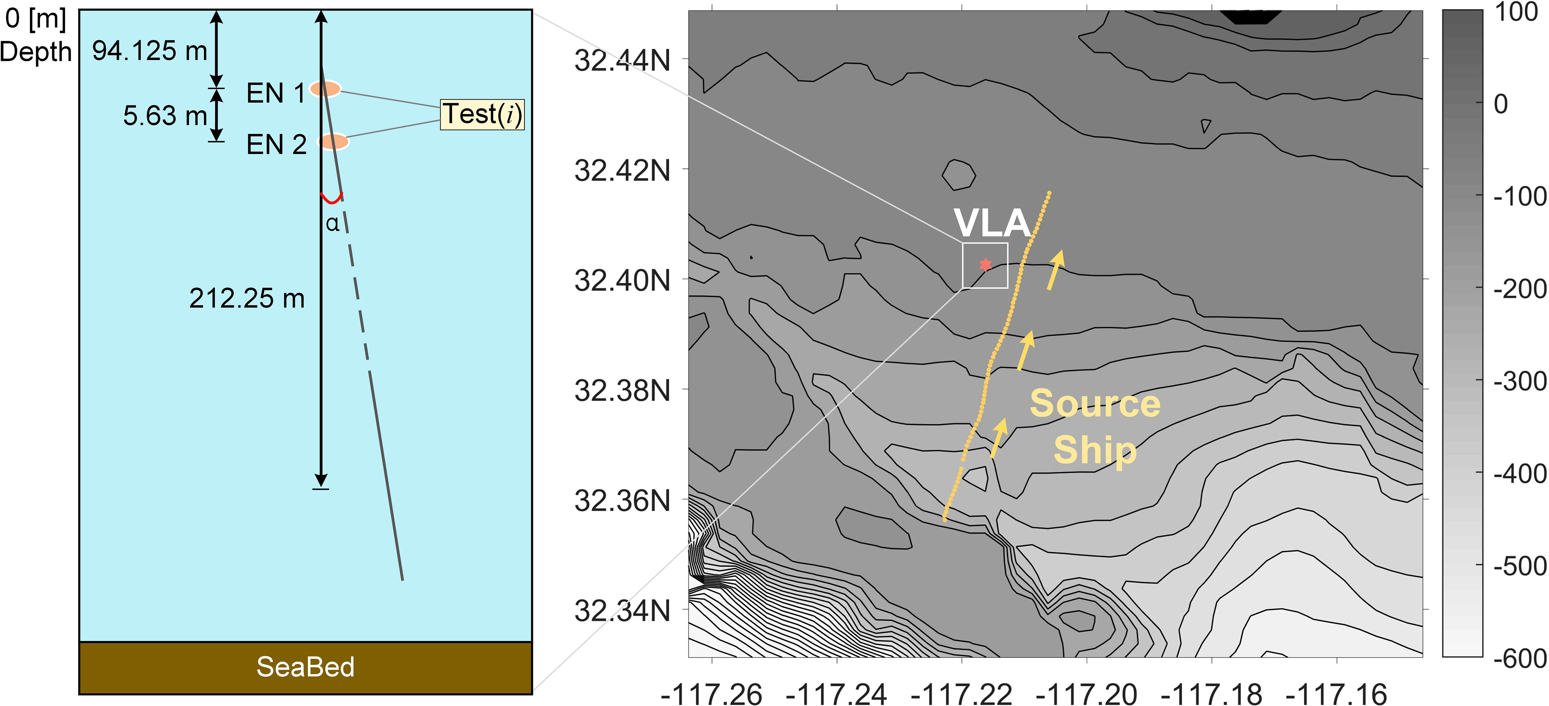
Figure 1 The study area near San Diego, California. The red dot marks the recording position VLA (32°40.254’ N, 117°21.620’ W) with a slight skew α, the yellow line is the track of the source ship from south to north, and the filled rectangle is defined as hydrophone signals selected as the data source for this CIAT.
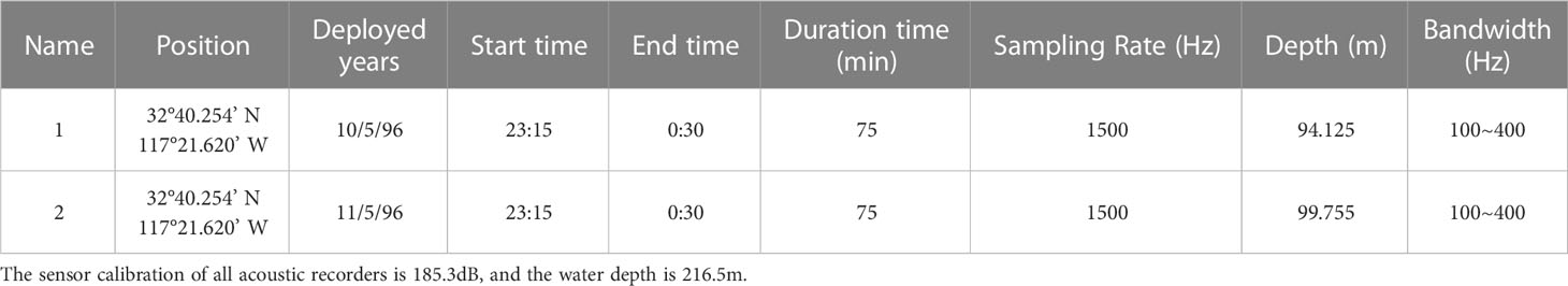
Table 1 Overview of analytical acoustic data recorded by two acoustic recorders.
From Figure 2, it is evident that there are many similarities between the acoustic signals of the sound source ship and bowhead whales. Specifically, there is a clear comb-like structure at the vocalization of the bowhead whale, which corresponds to the sound source ship. What’s more, both the radiated signal from the sound source ship and the calls of whales share common characteristics such as uniform background noise and being considered quasi-steady-state processes in the short term. To fulfill the validation requirements of this study, the SW-96 experimental data is well-suited. Hence, this study employs acoustic data resembling whale signals to assess the feasibility of CIAT. As the availability of measured data is limited, synthetic data will be used to complement the CIAT data preparation. Detailed data information can be found in Table 2.
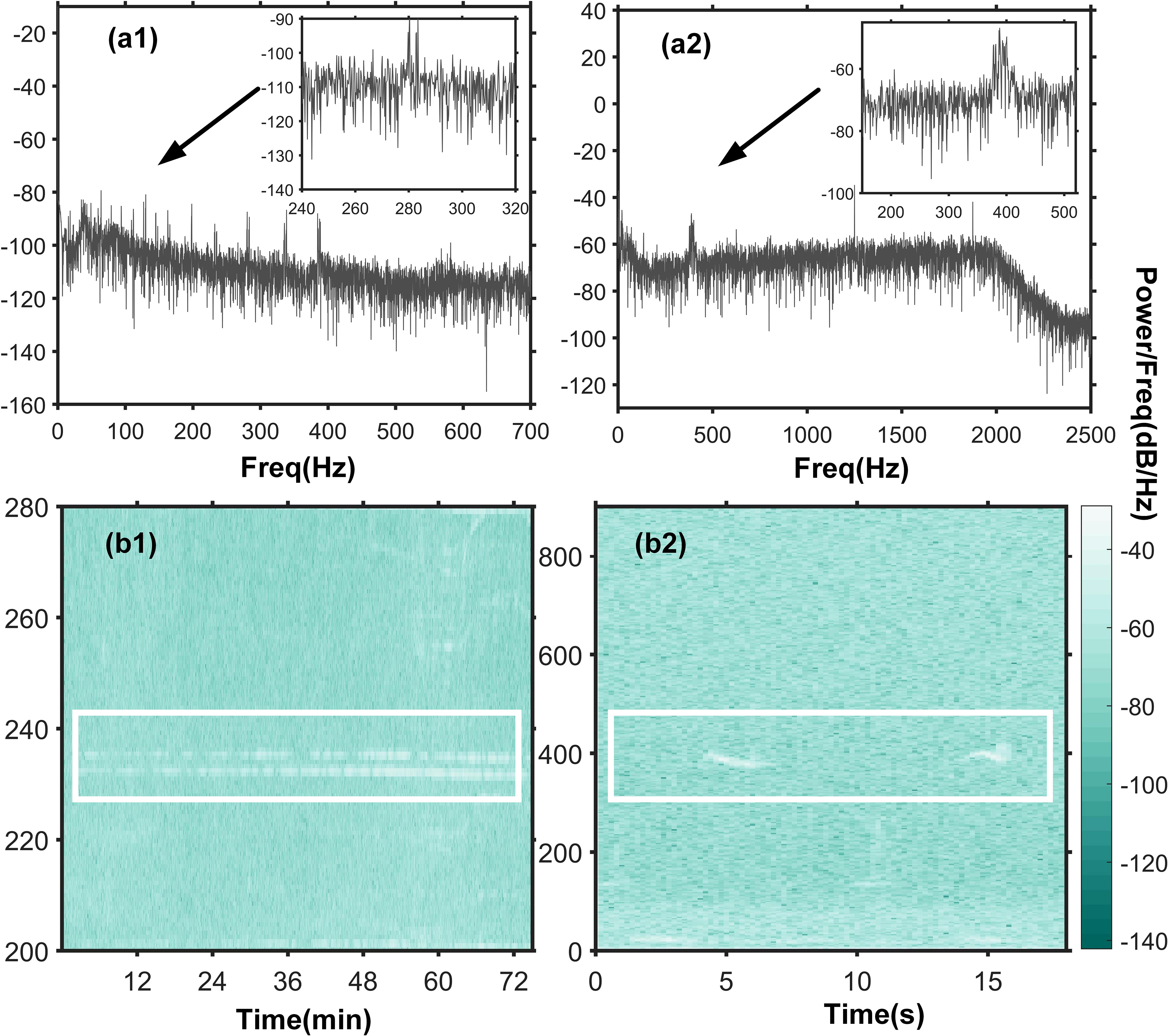
Figure 2 Power spectrum and time-frequency plots of the received signal from No. 1st hydrophone and the bowhead whale signal. (A1) The power spectrum of the signal received by No. 1st hydrophone, and (B1) the time-frequency diagram. (A2) The power spectrum of the bowhead whale, and (B2) the time-frequency plot. Data source NOAA Ocean Passive Acoustics Data Recorded by instrument NRS01 (72.443N, 156.602W) under the mooring platform.
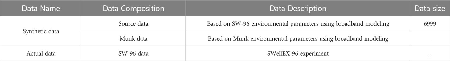
Table 2 Data description.
Synthetic data are generated through broadband modeling based on normal wave theory. Normal wave model is a classic sound field model, which mainly studies the amplitude and phase changes of sound signal in the sound field. It is suitable for far fields such as low frequency, shallow sea, constant level and other far fields. The solution is expressed as an integral solution in the wave equation. KRAKEN (Byun et al., 2019) uses the finite difference method to discretize the continuous problem in the wave equation, and the resulting solution is as follows:
where, r is the horizontal distance, is the depth, represents the density of seawater, zs represents the depth of the sound source, and ψ(zs,rl) is a constant and is the lth order normal wave.
The waveguide environment is simulated by the KRAKEN simulation program, and the parameters refer to the SW-96 or Munk experiment. And set the placement depth of the simulated sound source to 9m and the distance between the two hydrophones to be 150m. After calculating the sound pressure values of the broadband receiving space points, the solution of the time-varying wave equation is obtained by the Fourier synthesis method of the frequency domain solution. By doing so, uninterrupted time domain reception signals for both hydrophones are generated.
where, S(ωk) is the sound source spectrum; is the number of FFT points, and the transmission frequency (ωk) is {109, 127, 145, 163, 198, 232, 280, 335, 385}.
According to Risoud et al. (2018), azimuth, distance and depth are the three key parameters for sound source localization. However, it is important to note that azimuth estimation and distance/depth estimation are different types of tasks that may require different model architectures and feature representations. Traditional algorithms, such as cross-spectral analysis, are commonly used for azimuth estimation by analyzing the phase information of the sound signals (Li et al., 2019). In contrast, deep learning models have powerful feature learning and expressive capabilities, which can effectively capture distance- and depth-related patterns and features in sound signals. To simplify the training and inference process of the model and improve the accuracy of parameter estimation, we will estimate these parameters separately using their respective features and information. Doing so avoids introducing data association problems and redundant information. Our proposed model combines three key technologies: unsupervised learning algorithm based on enhanced cross spectral analysis, CNN and transfer learning (Ramírez-Macías et al., 2017; Fortune et al., 2020; Kovacs et al., 2020), and Figure 3 shows the CIAT flowchart.
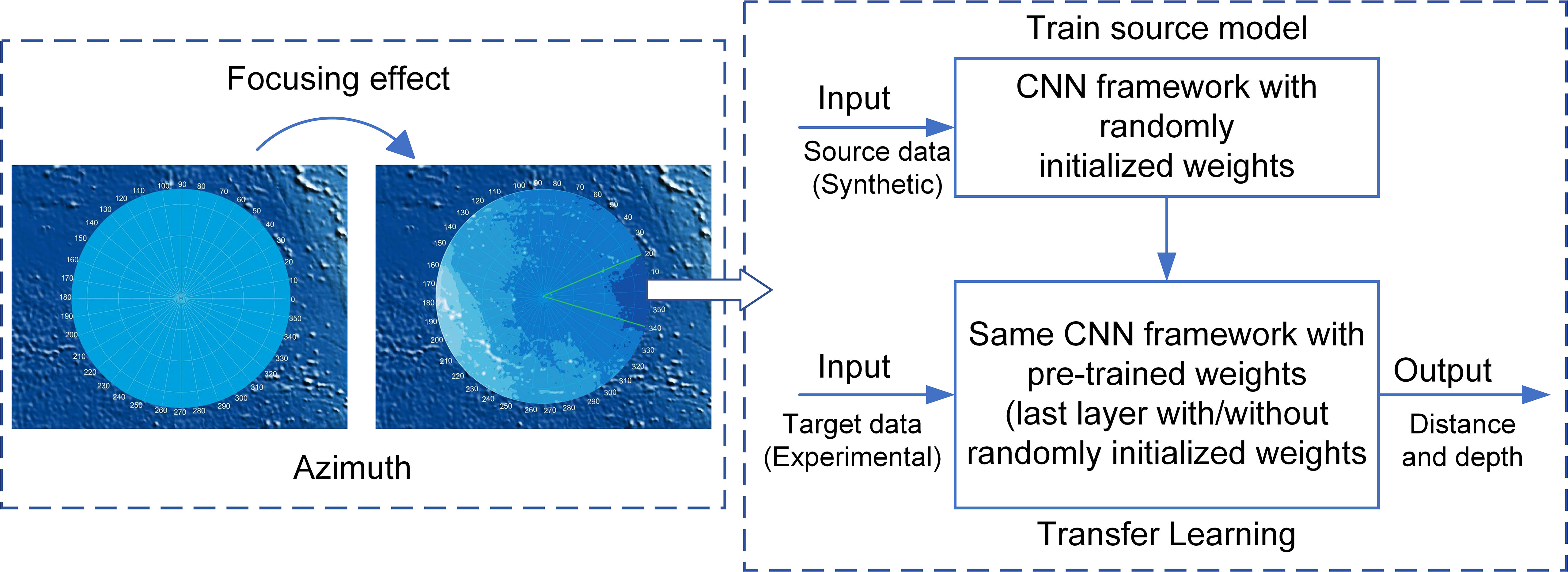
Figure 3 Schematic diagram of the overall architecture of CIAT.
It can be seen from Figure 3 that CIAT begins by using the improved cross-spectrum analysis method to determine the direction of the sound source and can effectively focus on the position of the sound source, which helps to improve the accuracy and robustness of the sound source localization. Subsequently, employ a combination of CNN and transfer learning to estimate the distance/depth of the sound source. By using the CNN model, we can extract features about the depth and distance of sound sources from the input signal. Transfer learning allows us to leverage models pre-trained on other related tasks, thereby accelerating the convergence of the network and improving performance. Finally, the azimuth estimation and the distance/depth estimation results are integrated to realize the trajectory prediction. Figure 4 shows a detailed overview of the steps involved in the process.
Step 1: Enhanced cross-spectral analysis is used to get the horizontal azimuth. We calculate the cross-spectral values of the time-domain data within the frames, and then filter the spectral peaks of the frequency points to get the target angle information. Compared with traditional algorithms, this unsupervised learning algorithm eliminates the interference of non-source signals and the multiple solutions of CIAT.
Step 2: A pre-trained model is built based on the CNN algorithm to mine signal-spatial features. The source data of ambient-field spatial features are reconstructed using broadband modeling, and more unpredictable features between the received signals and the target positions are mined by establishing a signal-spatial transfer mechanism. Compared with the traditional beamforming technology, the pre-trained model could directly perceive the signal-spatial features instead of indirectly extracted phase and frequency features.
Step 3: Use transfer learning to increase the generalization ability of the CIAT model. The convolutional layers of the pre-trained model are frozen by transfer learning to preserve the effect of signal-spatial feature perception in a specific application environment (Xu and Vaziri-Pashkam, 2021; Bedriñana-Romano et al., 2022; Dumortier et al., 2022). Small-domain discrete actual data is added to the target environment to strengthen the non-mapping connection between the fully connected layer features and the actual target locations. The CIAT model could adapt to dynamic perturbations in the marine environment, significantly improving tracking accuracy.
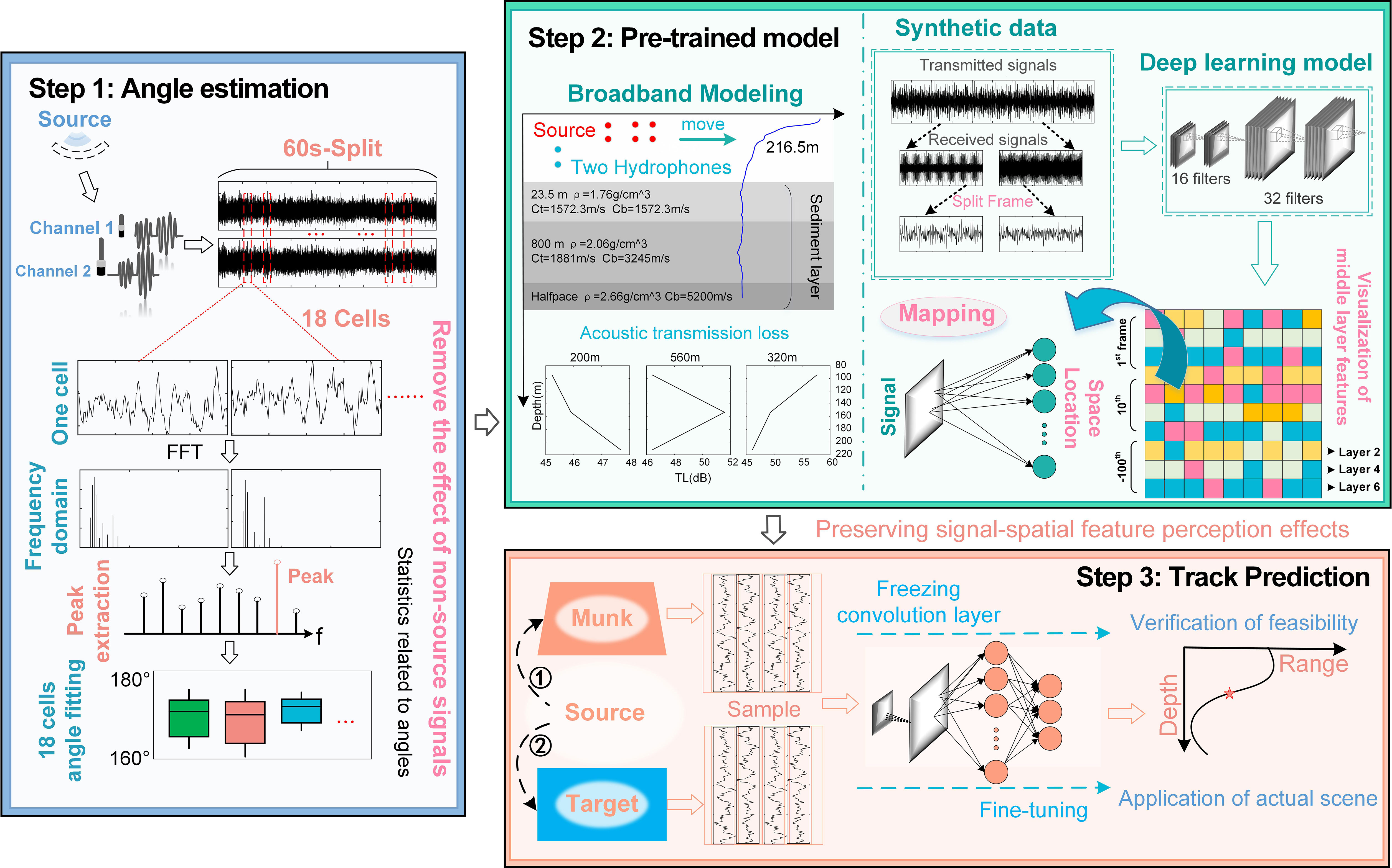
Figure 4 A detailed overview of the three steps performed by CIAT.
Based on the received signals from the two hydrophones, the azimuth of the sound source is first calculated using an enhanced cross-spectrum analysis. Then a pre-trained model is built using CNN algorithm to infect signal-spatial features. Finally, transfer learning is combined to enhance the generalization ability of the CIAT model.
The cross-spectrum method utilizes the principle of signal correlation (Virovlyansky, 2020; Lo, 2021) and can effectively suppress noise. Let s1(t) and s2(t) be the broadband signals received by the two hydrophones, then the cross energy spectral density is expressed as:
where, F1(f) and F2(f) are the spectral density functions of s1(t) and s2(t), respectively. According to the time delay characteristics of the Fourier transform, the time delay information is included in the phase information of the cross spectrum, then the phase of the cross-spectrum density at the frequency f is:
For a wideband signal with a bandwidth of B, in order to improve the accuracy of the phase difference measurement, we divide the time-domain received signals of the two hydrophones into frames, and calculate the cross-spectrum value of each frame separately. Then calculate the phase difference of each frequency sampling point in the signal bandwidth according to the above formula, and take the maximum value as the accurate phase difference of the center frequency sampling point to calculate the azimuth angle of the incident signal. Without considering the phase ambiguity, the maximum phase difference is:
where, . The improved cross-spectral analysis method estimates the azimuth of the target by taking the frequency point corresponding to the maximum spectral value. Compared with the traditional cross-spectrum method, the method effectively eliminates the interference of non-source signals, thereby significantly improving the direction-finding accuracy.
CNN is one of the most powerful deep learning architectures that can automatically extract necessary features from raw data without any hand-crafted features. It has gained popularity in various fields such as image recognition, speech recognition, and natural language processing. In addition, the main reasons for using dual-channel end-to-end training are as follows. (1) the input is provided by raw audio data recorded by two hydrophones, which allows it to perform joint feature learning with passive whales, avoiding manual feature selection. Meanwhile, (2) an end-to-end data-driven approach brings us the possibility to capture more complex spatiotemporally correlated latent features of the two hydrophones through the main convolution operation (Chen and Schmidt, 2021; Dayal et al., 2022).
Table 3 shows the size and number of convolutional filters in the proposed topological network. Adding a batch normalization layer after the input layer enhances the training process by reducing the drift of the input data distribution. This normalization technique accelerates network training by ensuring more stable gradients and mitigating the impact of varying input distributions. By normalizing the activations within each mini-batch, batch normalization promotes faster convergence and improves the overall efficiency of the network, and then concatenates two identical convolutional blocks. From an audio signal processing perspective, a convolutional unit can be viewed as a set of finite impulse response (FIR) filters with learnable coefficients, allowing more complex and comprehensive sample latent features to be extracted from large-scale data. The max pooling operation preserves more important features. The same is true for the remaining two convolution blocks. The “distributed features” are flattened and fed into a fully connected hidden layer of 100 units, designed to integrate and arrange the content in the filtered acoustic signal to obtain the final function as a solution.

Table 3 CIAT parameters.
where H() is the calculation process of a complete hidden layer. s is the time domain acoustic data of two hydrophones. Fout(x)= Act(ωx + b) represents the fully connected layer, where w and b are the parameters of the fully connected layer. ReLU activation function is used in all layers except the output layer to ensure that all outputs are positive and reduce the risk of gradient explosion and gradient disappearance during network training. In each training round, the model is optimized for accuracy using the Adam algorithm.
In CIAT, we build the target models using exactly the same architecture as the pre-trained (Zhong et al., 2021) models and use the parameters of these pre-trained models (except for the parameters of the output layer) as initial parameters. These transferred models are then retrained using small samples of actual data, a process called fine-tuning. Different transfer learning experiments are also performed to test the robustness of the transfer learning scheme by passing only some parameters of the hidden layers or fine-tuning the parameters of the selected layers, and the model performance was evaluated using the same approach. Here, we demonstrate that even using a small experimental training set, it is possible to extract significant signal-spatial features by expanding the dataset with computer-generated raw acoustic data.
Model performance metrics for Mean Absolute Error (MAE), Root Mean Square Error (RMSE) and Correct Positioning Ratio (CPR) are defined as below:
where N is the number of test sets, r is the real distance, and is the predicted distance; d is the real depth, and is the predicted depth. The smaller the MAE and RMSE, the better the performance, and the larger the CPR value, the better the model performance. These three indicators can intuitively reflect the closeness of the predicted result to the true value (Masmitja et al., 2020; Fonseca et al., 2022; Guzman et al., 2022; Skarsoulis et al., 2022).
The azimuth estimation process refers to Step 1 of the Model Architecture. We use enhanced cross-spectral analysis to obtain the target horizontal azimuth information. The local northeast coordinate system is established with the 1st hydrophone of the HLA as the origin, and the relative coordinates of other positions are recalculated by Universal Transverse Mercator Grid System (UTM) transformation to obtain the actual azimuth (blue line in Figure 5A). To determine the mutual spectral values of the two signals, two hydrophones of VLA (Chambault et al., 2022; Yang et al., 2022) are chosen to record time-domain data in frames. Assuming the normal direction of the line connecting the 1st hydrophone and the sound source ship at the 60th minute is 0°, the azimuth angle less than 60min is θ, and the azimuth angle more than 60min is 180°-θ.
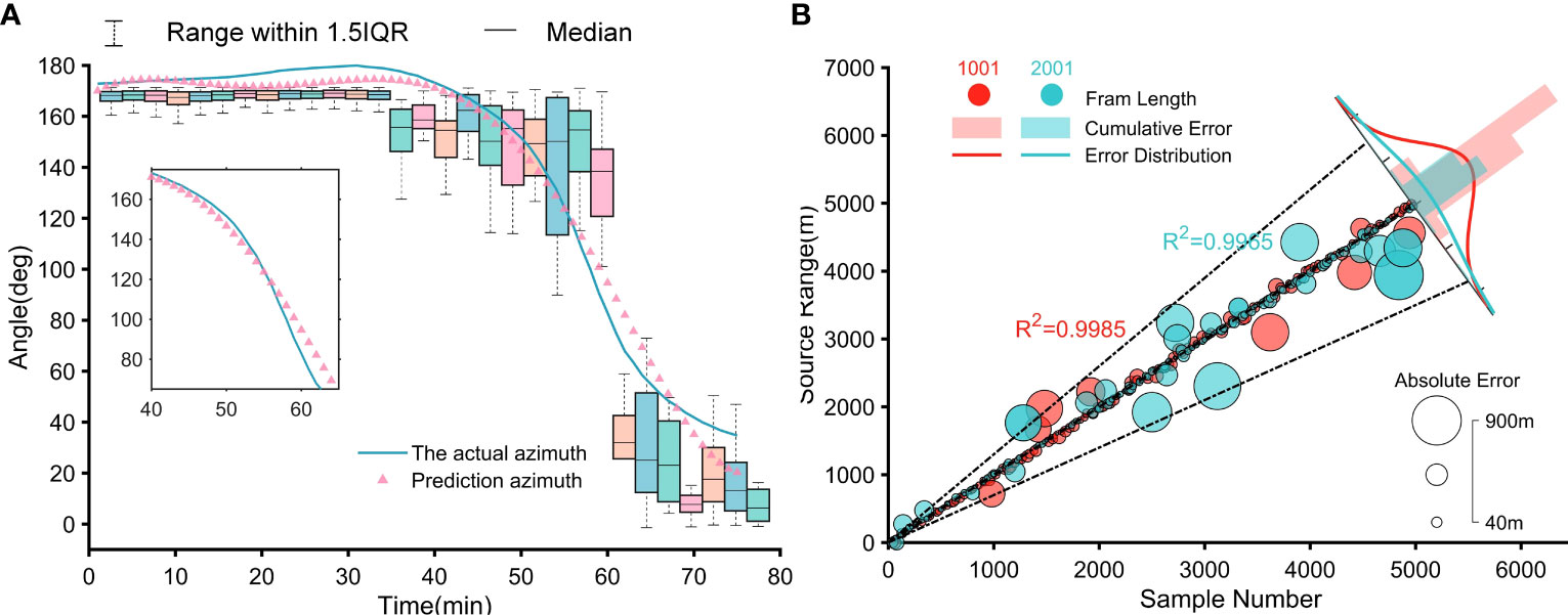
Figure 5 Estimation results. (A) SW-96 experimental data azimuth estimation. (B) Comparison of distance estimation results for pre-trained model frame lengths of 1001 and 2001.
Due to the similarity in average spectral values of the signals captured by the two hydrophones, the traditional cross-spectrum analysis method faces challenges in distinguishing them. As a result, the calculated angle tends to be either 0 or NaN (not a number), indicating that it cannot be reliably determined due to the similarity in average spectral values. Compared to conventional spectral analysis algorithms, our enhanced cross-spectral analysis ensures the accuracy of azimuth estimation by finding the spectral peaks corresponding to the main frequency points. This unsupervised learning algorithm maintains the intrinsic connection between the two received signals, eliminates the influence of non-source signals, and ensures the unique solution and objectivity of CIAT.
In Figure 5A, the boxplot visually represents the distribution and dispersion of the azimuth data. It effectively summarizes key statistics such as medians, quartiles, etc., providing insight into the central tendency and variability of azimuth values. Additionally, the scatterplot in the same figure shows azimuth data obtained from a fifth-order polynomial fit, which reveals patterns and trends exhibited throughout the specified time period. As seen in detail (Table 4), particularly, the Absolute Error (AE) in the angle exceeds 10° at about 59 minutes. This phenomenon that the azimuth error is the largest when the target is closest to the hydrophone is consistent with the results of Watkins and Schevill et al., which confirms the effectiveness of our horizontal azimuth estimation algorithm and further boosts the credibility of our intelligent acoustic tracking model.
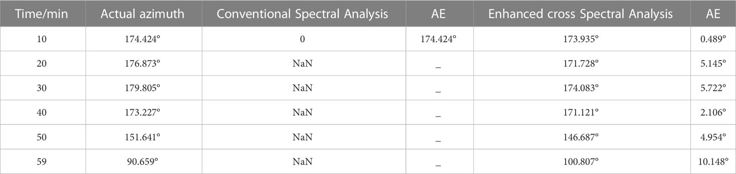
Table 4 Azimuth estimation results.
Distance/depth estimation includes CNN pre-trained model and transfer learning. First, the pre-trained model of CNN is built for processing received signals. The input of the model is N * 2 * S dimension, where N represents the signal sample length, 2 denotes the number of channels, and S represents the signal frame length. To ensure compatibility and optimize performance, we implement the entire framework using the Python programming language and the TensorFlow library on a Windows 10 x64 system. Compared to large networks like U-Net, CNN has a shallow network structure that does not require many parameters to train its performance. This characteristic has led our model to outperform most previously used models in this research area.
The frame lengths 1001, 2001, and 3001 all demonstrate conformity to the normal distribution as predicted by the theory, thus verifying the validity of the model and its prediction accuracy. Notably, the frame length of 1001 exhibits the highest accuracy in predictions (Figure 5B). Since the underwater depth of the whales is almost constant during migration, this paper does not place a high value on depth changes. For the frame length of 1001, the distance estimation errors within 6 km are 0.0322 km/MAE, 0.0805 km/RMSE, and 94.57%/CPR. The above fully illustrates that our CNN pre-trained model could directly perceive the signal-spatial features.
We visualize the trend changes of weights acting on 16 convolutional kernel units in the first layer of the dual-channel system. Figure 6 illustrates this, where (a) represents the weight values of 16-1; (b) 16-2; (c) 16-3; and (d) 16-4. The shaded regions indicate perfect recordings when both sound waves arrive simultaneously, otherwise, they indicate a delay. From Figure 6, we can infer the following:
1) The trend changes between different weights reflect the time difference or phase difference of the sound waves reaching the two hydrophones. The weights show significant changes or overlaps at specific positions. For example, at the upward-pointing Perfect shaded arrow, we can infer that the time or phase difference of the sound waves’ arrival is small.
2) The differences between different weights can reflect the variations in the signals received by the two hydrophones. If the weights exhibit noticeable differences at certain positions, such as the right-pointing Delayed shaded arrow, it suggests significant discrepancies in the signals received by the hydrophones at that position.
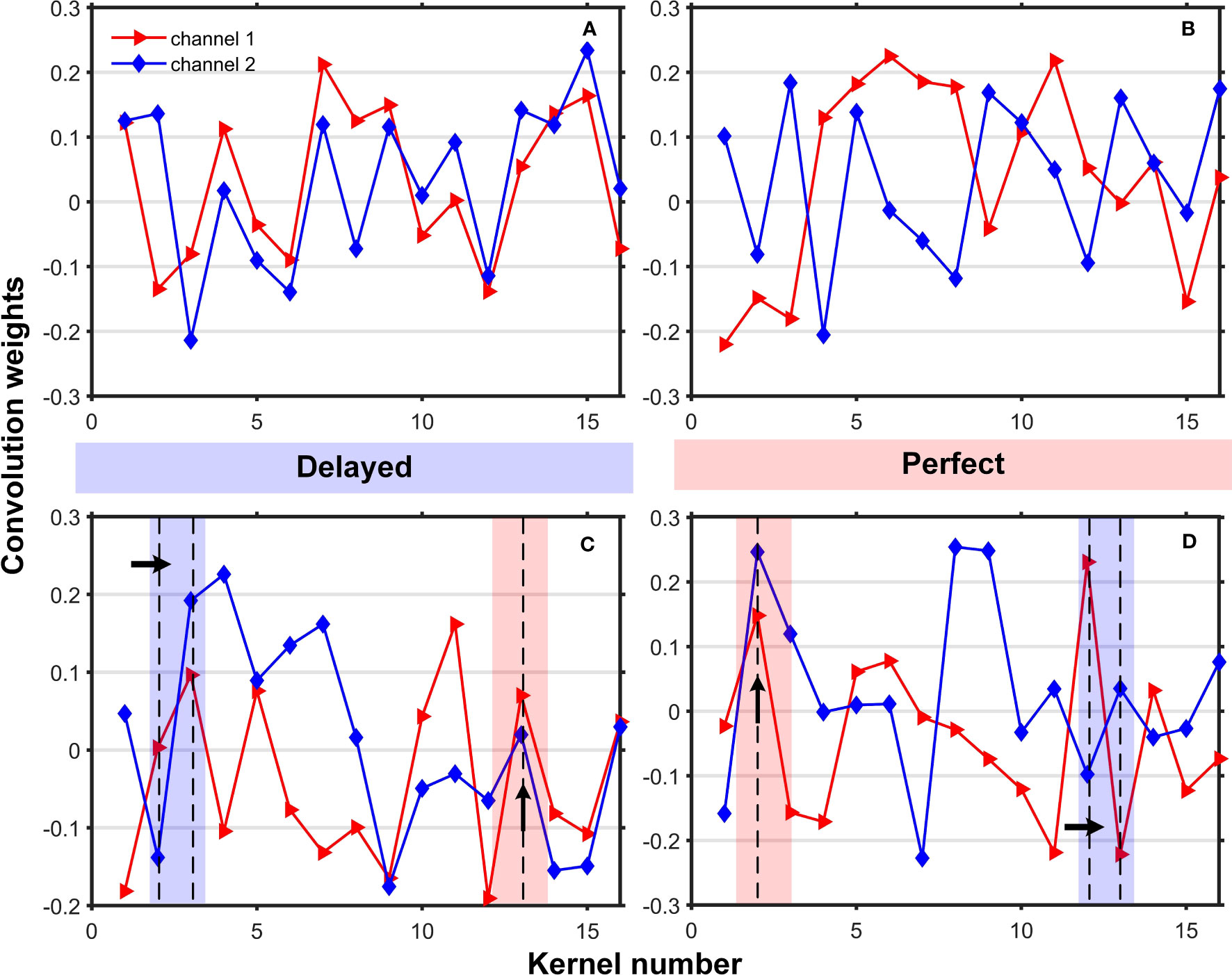
Figure 6 Respectively act on the weights of the dual-channel convolution kernels. (A) represents the weight value of 16-1; (B) 16-2; (C) 16-3; (D) 16-4. The shaded areas represent: two sound waves arriving at the same time are recorded as Perfect, otherwise, Delayed.
By considering the combined trend changes and differences in weights, we can deduce that the signals received by the two hydrophones have different arrival times and phase differences, and there are significant discrepancies at certain positions. This aligns with the actual scenario of sound propagation reaching the two hydrophones, thereby enhancing the model’s interpretability and reliability.
Further, Figure 7 provides insights into the intermediate layer feature representations of CIAT. When examining the signal features of different time frames (signals 1, 2, 3), the features extracted from the last 100 frames are slightly better than those extracted from the first and tenth frames. The reason behind this observation is that the initial time period predominantly captures the direct path sound signal, which does not exhibit a distinct multipath reflection signal pattern. As the network layers deepen, the extracted features become more specific and sparser, indicating the presence of spatial selective gradients within CIAT. Comparing (a) and (b) in Figure 7, without transfer learning (marked by ellipses), the obtained features are blurry, and even with increasing network layers, the features extracted from two similar time frames remain indistinguishable. However, through transfer learning (marked by rectangles), the learned features are not only representative but also avoid the issue of feature blurriness.
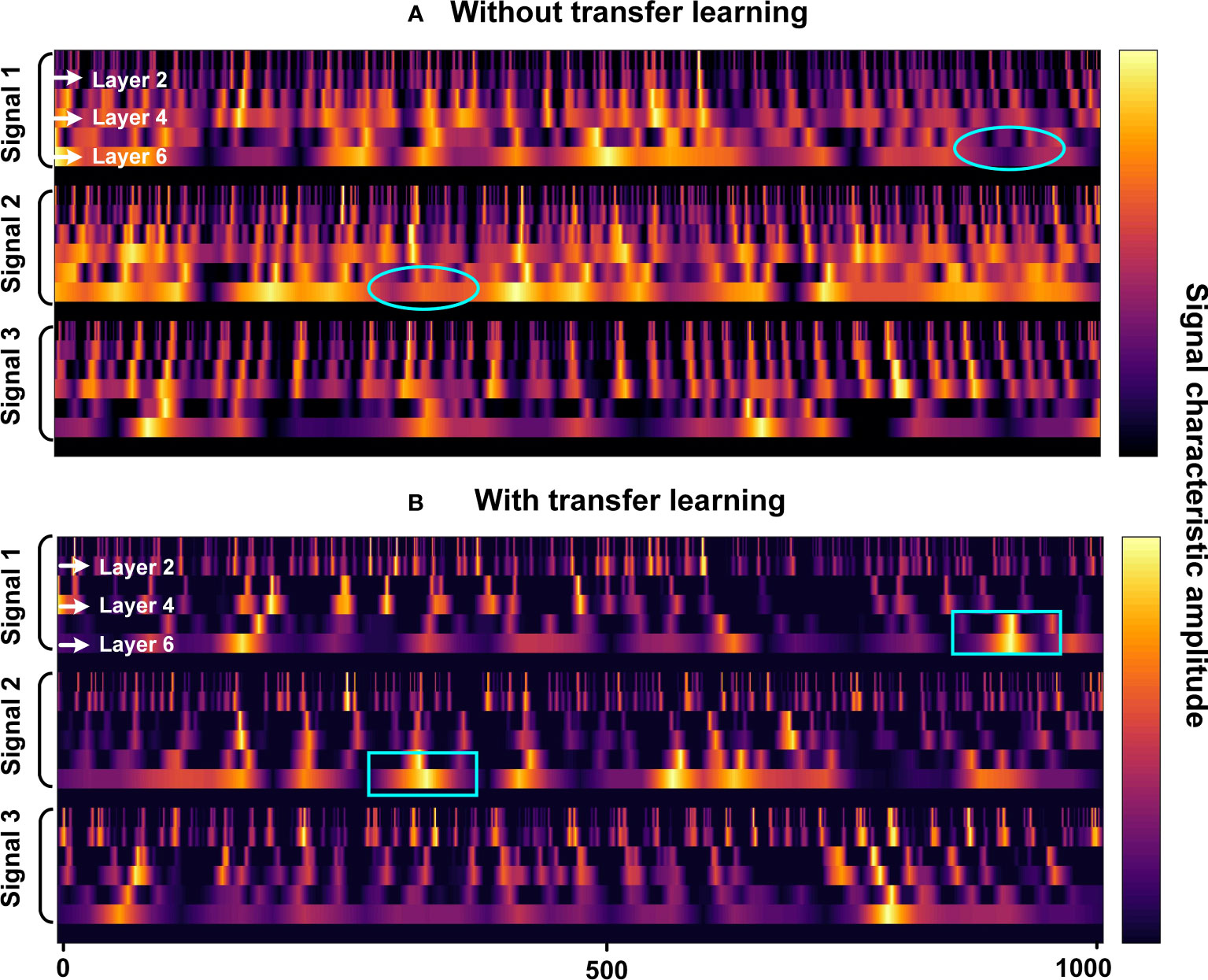
Figure 7 The middle layer feature representation for CIAT. (A) Without transfer learning; (B) With transfer learning.
The observations strongly suggest that CIAT is capable of extracting signal features from various time frames through a nonlinear feature extractor. Additionally, the model exhibits good generalization capabilities when applied to real-world data. These findings lay a solid foundation for the potential success of using CIAT in tracking whales during migration.
Next, the signal-spatial feature parameters of our pre-trained model obtained in the ideal environment are applied to the target environment by transfer learning to evaluate the effect of the target model on the perception of the actual received signal features (Gemba et al., 2017; Worthmann et al., 2017; Agrelo et al., 2021; Coli et al., 2022). The target model’s input is Munk-based synthetic data to determine the effective transfer of signal-spatial feature mechanism, thus ensuring the feasibility of the proposed model. After that, the CNN pre-trained model’s convolutional layer is frozen. However, this frozen CNN pre-trained model does not serve as the final model for the effect of dynamic ocean perturbations, which would result in an environmental mismatch between the source and target model datasets. Therefore, we use transfer learning to share the weight parameters of the CNN pre-trained model and put small sample data to the target model for achieving accurate prediction positions by fine-tuning the fully connected layer and setting Dropout 0.5 to build the Munk target model.
The estimation errors of the Munk target model are 0.015km/MAE and 97%/CPR (Figure 8A). It can be seen that the predicted distance of the target in the Munk environment is consistent with the actual distance, indicating that our transfer learning algorithm could make the model’s generalization performance enhanced and adapt to different environments with guaranteed accuracy. In addition, we test the reproducibility of the transfer algorithm by changing the signal pattern of the source from comb to FM emission and also set Dropout 0.3. Figure 8B shows that the distance estimation errors are 0.031km/MAE and 93%/CPR, which also has high accuracy and proves the robustness of the CIAT.
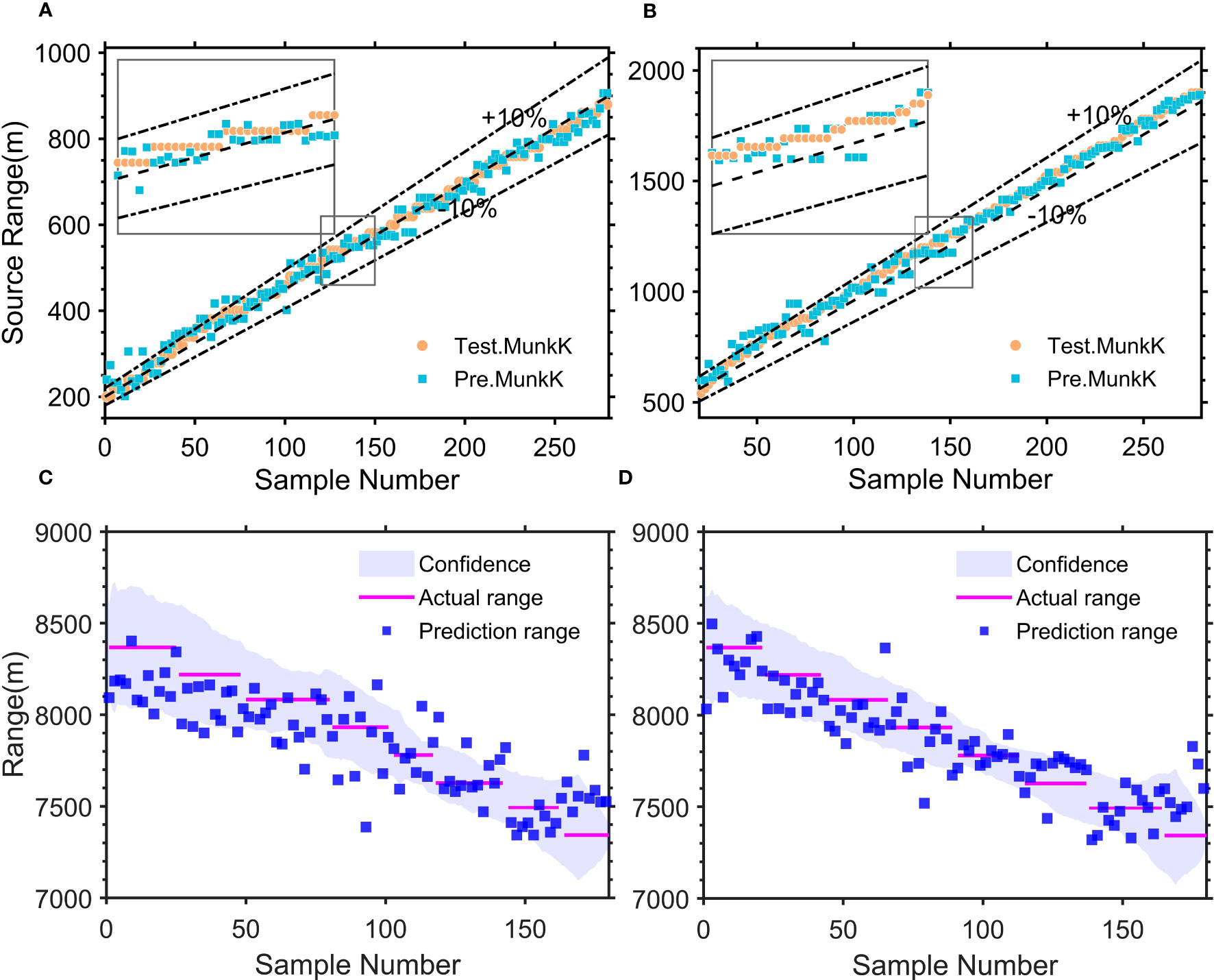
Figure 8 Positioning and tracking results. (A) Distance estimation results for synthetic data of the Munk environment, and (B) results for the change of signal form to FM signal. (C) The prediction result of SW-96 experimental sound source distance without transfer learning, and (D) with transfer learning.
Next, we apply this transfer algorithm to the actual experimental data with ambient noise and reverberation. Based on our frozen CNN pre-trained model, the first 9 minutes of raw acoustic data from two hydrophones are used as the input to the SW-96 target model, and two Dropout layers (0.5 and 0.1) are added to complete the sound source ship distance/depth prediction. As shown in the distance results, the estimation error of distance obtained within 8 km without transfer learning is 0.15 km/MAE (Figure 8C), while with transfer learning the distance estimation errors are 0.13 km/MAE, 0.164 km/RMSE, and 100% CPR, respectively (Figure 8D), demonstrating that the distance prediction accuracy using transfer learning at sparse data is higher than that without transfer learning. And Figure 9A shows that the predicted depth of the target in the SW-96 environment is consistent with the actual depth. Besides, in the same experimental environment, we also compare CIAT and traditional matching field processing (MFP) techniques (Wang et al., 2020). The results are shown in Table 5, which shows that the traditional method is severely limited by multipath propagation and spatial correlation in the marine environment, and it cannot complete the tracking task solely by relying on two hydrophones. These further verify that our proposed model only based on two hydrophones can adapt to the effects of dynamic marine environmental perturbations brought about by scene switching and can be extended to applications in actual marine environments.
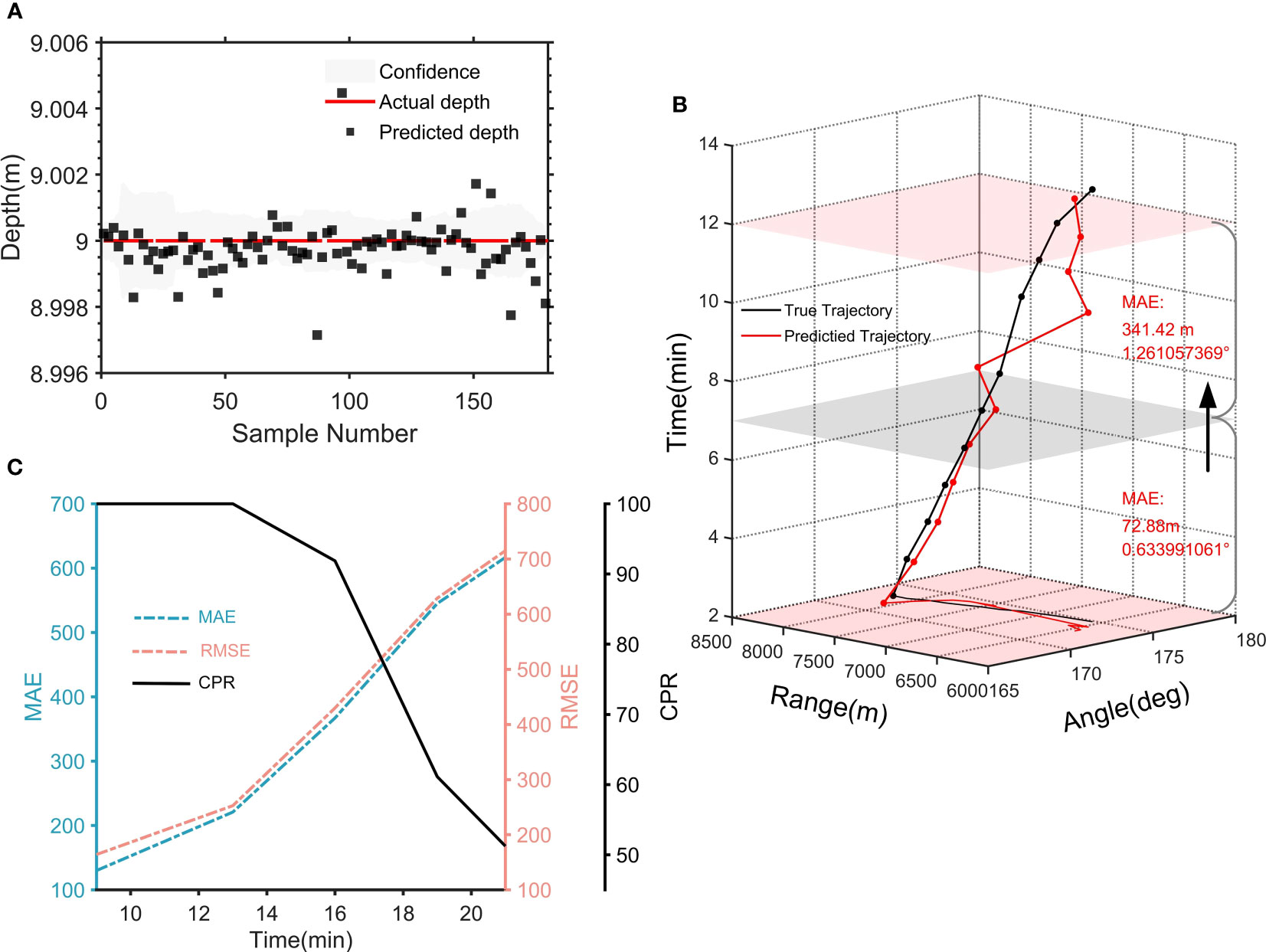
Figure 9 Tracking results. (A) Depth estimation results. (B) Tracking trajectory of the sound source ship. X-axis the distance of the source ship from the 1st hydrophone, Y-axis the azimuth of the source ship, and Z-axis the time dimension. Green line the real trajectory and the orange line is the predicted. (C) The three indicators of MAE, RMSE, and CPR verify the accuracy of the CIAT model, and show the trend of the indicators as time increase and evaluate the generalization ability of the model.
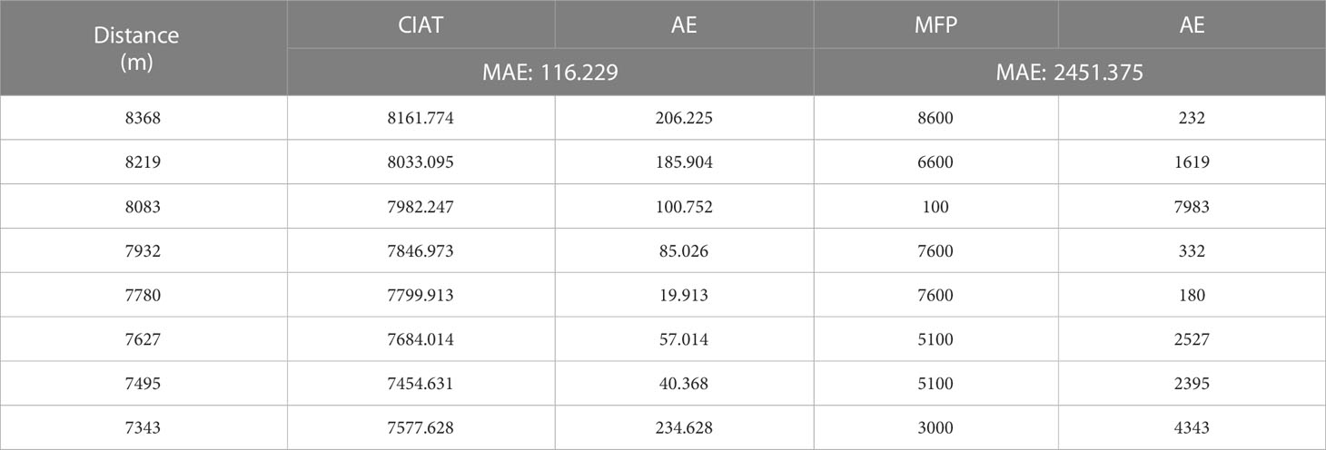
Table 5 Comparison results of CIAT and MFP.
Our model enables to perform high-precision tracking in both Munk and SW-96 actual environments, and it is a key advantage of our CIAT to achieve high-precision tracking at 8 km 0.13 km/MAE in actual marine environments using two hydrophones. At the same time, CIAT can also adapt to switching between different marine environments like Munk and SW-96, but since both CNN and transfer learning in CIAT are black-box models, there is currently no effective physical mechanism to explain this phenomenon. Therefore, another important direction of our work focuses on explaining the physical mechanism of CIAT to support switching between different marine environments.
Theoretically, our CIAT is mainly affected by the ambient noise and ocean reverberation that exist in different marine environments when applied. However, since the source dataset is synthetic data used for broadband modeling, it is determined that the features shared will not be ambient noise.
From the SW-96 experimental results, the CIAT is directly applied to sound source distance/depth estimation after the first 9 minutes of transfer training. The statistical errors of the predicted 10-16 min distance are 0.367 km/MAE, 0.429 km/RMSE, and 91.87%/CPR, while the statistical errors of 10-19 min are 0.545 km/MAE, 0.628 km/RMSE, and 61.13%/CPR, and the effective time of the model tracking time is longer than 7 min (Figure 9B). From the measured data MAE, RMSE and CPR (Figure 9C), these three performance indicators can show that the error of CIAT increases with increasing tracking time, demonstrating that the spatial characteristics of the transmitted signals belong to the time domain. Additionally, as tracking time increases, various interface scattered acoustic waves are continuously superimposed in the hydrophone signals, also exhibiting time-domain characteristics. Therefore, we believe that the signal-spatial features conveyed by the transfer learning of CIAT are oceanic reverberations, which are the physical mechanism of their ability to support switching between different marine environments.
Transfer learning in CIAT conveys the signal-spatial features that are ocean reverberations, which support the interpretation of switching between different marine environments. We then conducted two sets of experiments to further measure the ability of CIAT to adapt to such environmental differences.
Group 1: The spacing between the two hydrophones is fixed for different permutations.
As shown in Figure 10A, the prediction error distribution tends to be consistent, although the combination categories are not identical. Setting the distance to 5.63m, the prediction errors for different combinations are shown in Table 6, which proves that the signal-spatial features perceived by the pre-trained model are effectively transferred under a certain spacing. Therefore, the model can obtain accurate prediction results using 2 hydrophones under a certain spacing. This experiment illustrates that under a certain spacing, the change in spatial location has little effect on the adaptive ability of CIAT.
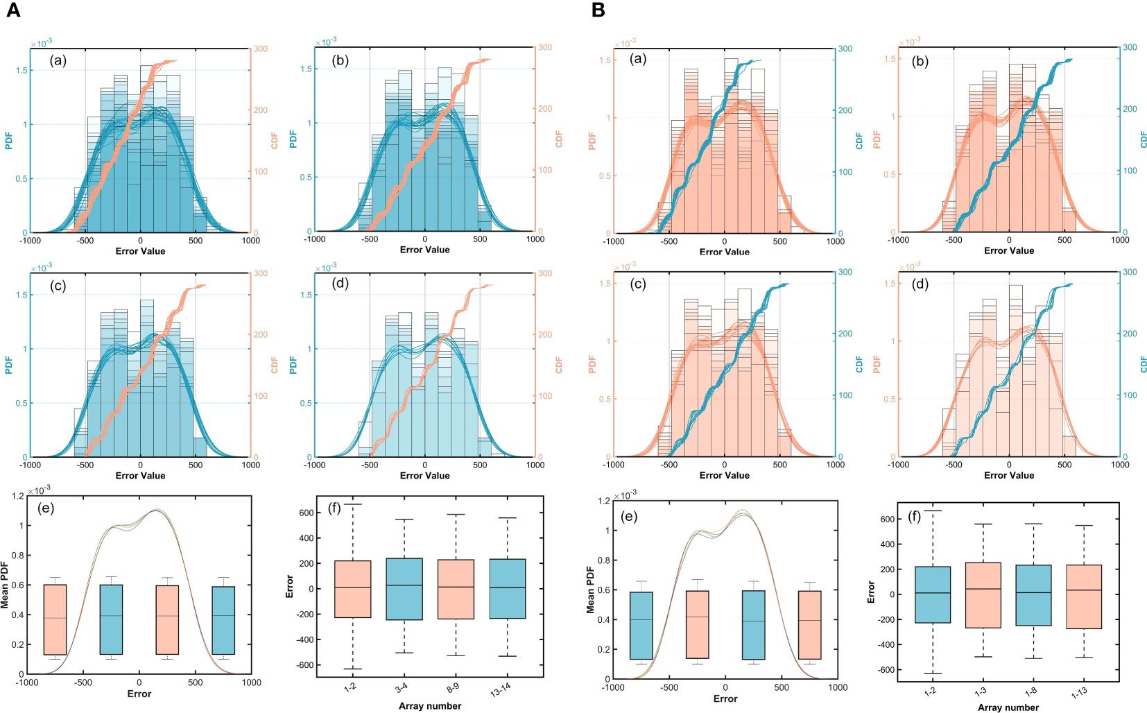
Figure 10 Prediction error distribution for repeated experiments. (A): (a) Error histogram, probability density function and cumulative distribution function of error points at 5.63m. (b) 19-11.26m. (c) 14-38.41m. (d) 7-67.56m. (e) and (f) Error distribution plots and the mean PDF. (B): (a) Error histogram, probability density function and error point cumulative distribution function for different hydrophone spacing, respectively. (b) 3-8 (c) 8-12 (d) 13-7 (e) and (f) Error distribution plots and the mean PDF.
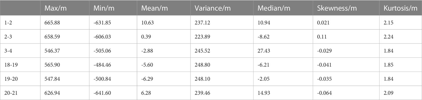
Table 6 Numerical statistical properties of errors.
Group 2. One hydrophone is settled, and the spacing between the two hydrophones is adjusted.
Figure 10B shows that the prediction error distribution still tends to be similar when the spacing between two hydrophones is changed. As shown in Table 7, the prediction errors fluctuate slightly without significant differences. This experiment illustrates that CIAT is still highly adaptable to the environment when the spacing and spatial location of two hydrophones are both changed.
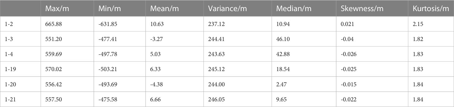
Table 7 Numerical statistical properties of errors.
In this study, we propose a composite intelligent tracking model (CIAT) to achieve both azimuth and distance/depth estimation with solely two hydrophones, thereby allowing complete and accurate tracking of whales, especially 0.13 km/MAE within the range of 8km. It addresses that the current spatial-temporal correlation techniques are limited by the hydrophone quantity accumulation, arrival time sensitivity and low tracking accuracy. Additionally, another important direction of our study focuses on explaining the physical mechanism of CIAT to support switching applications in different marine environments.
For the horizontal azimuth estimation, we use the enhanced cross-spectral analysis based on unsupervised algorithm to overcome the problem that traditional methods are seriously affected by non-source signals and multiple solutions of CIAT. We calculate the cross-spectrum values of the time domain sub-frames of the two hydrophone received signals, and then estimate the azimuth of the target based on the obtained spectral peaks of the corresponding frequency points. The results demonstrate that the minimum error reaches 0.489° and the average error is 4.762° within 75 min, which solves the failure of the traditional cross-spectral orientation methods and obtains the azimuth information with high precision.
For the distance/depth estimation, the spatial feature source data is reconstructed by broadband modeling to overcome the sparsity of the measured data. Then, a CNN pre-trained model is constructed to mine more obvious and robust features between the received signals and the target positions by establishing the signal-spatial transfer mechanism to avoid the dependence on indirectly extracted features such as phase and frequency.
Transfer learning is used to improve the generalization ability of CIAT model. For the Munk and SW-96 marine environments, the perceptual effects of signal-spatial features are preserved by freezing the convolutional layers of the CNN pre-trained model. Then small domain discretization of actual data is introduced to the target model to enhance the non-mapping relationship between fully connected layer features and actual target locations. The results demonstrate that our model exhibits generalization capabilities that enable it to adapt to changes in scene switching, hydrophone spacing, and signal reception form, and accurately predict target location information even with less data and unknown environmental conditions. Furthermore, from the perspective of theoretical analysis and repeatable experiments, it is demonstrated that the signal-spatial features transmitted by transfer learning are ocean reverberation. This is crucial to explain the physical mechanism by which CIAT enables to support switching between different marine environments.
Our proposed whale tracking model breaks the paradigm of improving tracking accuracy by accumulating physically “real” arrays, but fully senses and mines the unpredictable signal-spatial features of the two hydrophones for precise tracking. Especially, the transmitted signal-spatial features are found to be oceanic reverberations during the prediction process. This provides an explanation for the physical mechanism by which CIAT would be able to support switching applications in different marine environments. However, one of the most important limitations of this study is the small size of the training/validation set used. It is foreseeable that in the future, more acoustic received signal could be collected as an extension to provide more precise information for whale diversity conservation and stranding management.
The datasets presented in this study can be found in online repositories. The names of the repository/repositories and accession number(s) can be found below: http://swellex96.ucsd.edu/s5.htm.
JX and KJ conceived the study and coordinated the project effort. KJ and CL conducted the acoustic data analysis, tracking model validation, writing, and visualization. JX, KJ, XZ, CL, LX, and YL conducted the formal analysis, review, editing, and supervision. All authors contributed to the article and approved the submitted version.
This research was jointly supported by the National Natural Science Foundation of China (41706106).
We thank Ocean Acoustics laboratory members for critical reading of the manuscript and constructive suggestions during our research and Jim Murray formerly of the Marine Physical Lab for valuable SWellEx-96 experimental data.
The authors declare that the research was conducted in the absence of any commercial or financial relationships that could be construed as a potential conflict of interest.
All claims expressed in this article are solely those of the authors and do not necessarily represent those of their affiliated organizations, or those of the publisher, the editors and the reviewers. Any product that may be evaluated in this article, or claim that may be made by its manufacturer, is not guaranteed or endorsed by the publisher.
Agrelo M., Daura-Jorge F. G., Rowntree V. J., Sironi M., Hammond P. S., Ingram S. N., et al. (2021). Ocean warming threatens southern right whale population recovery. Sci. Adv. 7, eabh2823. doi: 10.1126/sciadv.abh2823
Ajala S., Muraleedharan Jalajamony H., Nair M., Marimuthu P., Fernandez R. E. (2022). Comparing machine learning and deep learning regression frameworks for accurate prediction of dielectrophoretic force. Sci. Rep. 12, 1–17. doi: 10.1038/s41598-022-16114-5
Aulich M. G., McCauley R. D., Saunders B. J., Parsons M. J. (2019). Fin whale (Balaenoptera physalus) migration in Australian waters using passive acoustic monitoring. Sci. Rep. 9, 1–12. doi: 10.1038/s41598-019-45321-w
Bedriñana-Romano L., Zerbini A. N., Andriolo A., Danilewicz D., Sucunza F. (2022). Individual and joint estimation of humpback whale migratory patterns and their environmental drivers in the Southwest Atlantic Ocean. Sci. Rep. 12, 1–16. doi: 10.1038/s41598-022-11536-7
Bursać P., Kovačević M., Bajat B. (2022). Instance-based transfer learning for soil organic carbon estimation. Front. Env. Sci. 10. doi: 10.3389/fenvs.2022.1003918
Byun G., Akins H., Song H. C., Kuperman W. A. (2019). Robust matched field processing for array tilt and environmental mismatch. J. Acoust. Soc Am. 146, 2962–2962. doi: 10.1121/1.5137294
Chambault P., Kovacs K. M., Lydersen C., Shpak O., Teilmann J., Albertsen C. M., et al. (2022). Future seasonal changes in habitat for Arctic whales during predicted ocean warming. Sci. Adv. 8, eabn2422. doi: 10.1126/sciadv.abn2422
Cheeseman T., Southerland K., Park J. (2022). Advanced image recognition: a fully automated, high-accuracy photo-identification matching system for humpback whales. Mamm. Biol. 102(3), 915–929. doi: 10.1007/s42991-021-00180-9
Chen R., Schmidt H. (2021). Model-based convolutional neural network approach to underwater source-range estimation. J. Acoust. Soc Am. 149, 405–420. doi: 10.1121/10.0003329
Coli G. M., Boattini E., Filion L., Dijkstra M. (2022). Inverse design of soft materials via a deep learning–based evolutionary strategy. Sci. Adv. 8 (3), eabj6731. doi: 10.1126/sciadv.abj6731
Davis G. E., Baumgartner M. F., Bonnell J. M., Bell J. (2017). Long-term passive acoustic recordings track the changing distribution of North Atlantic right whales (Eubalaena glacialis) from 2004 to 2014. Sci. Rep. 7, 13460. doi: 10.1038/s41598-017-13359-3
Dayal A., Yeduri S. R., Koduru B. H., Jaiswal R. K., Soumya J., Srinivas M. B., et al. (2022). Lightweight deep convolutional neural network for background sound classification in speech signals. J. Acoust. Soc Am. 151, 2773–2786. doi: 10.1121/10.0010257
Ding J., Ke Y., Cheng L., Zheng C., Li X. (2020). Joint estimation of binaural distance and azimuth by exploiting deep neural networks. J. Acoust. Soc Am. 147, 2625–2635. doi: 10.1121/10.0001155
Dumortier L., Guépin F., Delignette-Muller M. L., Boulocher C., Grenier T. (2022). Deep learning in veterinary medicine, an approach based on CNN to detect pulmonary abnormalities from lateral thoracic radiographs in cats. Sci. Rep. 12, 1–12. doi: 10.1038/s41598-022-14993-2
Ferreira R., Dinis A., Badenas A., Sambolino A., Marrero-Pérez J., Crespo A., et al. (2021). Bryde’s whales in the North-East Atlantic: New insights on site fidelity and connectivity between oceanic archipelagos. Aquat. Conserv. 31, 2938–2950. doi: 10.1002/aqc.3665
Fonseca C. T., Pérez-Jorge S., Prieto R., Oliveira C., Tobeña M., Scheffer A., et al. (2022). Dive behavior and activity patterns of fin whales in a migratory habitat. Front. Mar. Sci. 1134 (2022). doi: 10.3389/fmars.2022.875731
Fortune S. M., Ferguson S. H., Trites A. W., Hudson J. M., Baumgartner M. F. (2020). Bowhead whales use two foraging strategies in response to fine-scale differences in zooplankton vertical distribution. Sci. Rep. 10, 1–18. doi: 10.1038/s41598-020-76071-9
Frasier K. E., Garrison L. P., Soldevilla M. S., Wiggins S. M., Hildebrand J. A. (2021). Cetacean distribution models based on visual and passive acoustic data. Sci. Rep. 11, 1–16. doi: 10.1038/s41598-021-87577-1
Fu L., Zhang L., Dollinger E., Peng Q., Nie Q., Xie X. (2020). Predicting transcription factor binding in single cells through deep learning. Sci. Adv. 6, eaba9031. doi: 10.1126/sciadv.aba9031
Gemba K. L., Nannuru S., Gerstoft P., Hodgkiss W. S. (2017). Multi-frequency sparse Bayesian learning for robust matched field processing. J. Acoust. Soc Am. 141, 3411–3420. doi: 10.1121/1.4983467
Gupta V., Choudhary K., Tavazza F., Campbell C., Liao W. K., Choudhary A., et al. (2021). Cross-property deep transfer learning framework for enhanced predictive analytics on small materials data. Nat. Commun. 12, 1–10. doi: 10.1038/s41467-021-26921-5
Guzman H. M., Collatos C. M., Gomez C. G. (2022). Movement, behavior, and habitat use of whale sharks (Rhincodon typus) in the tropical Eastern Pacific Ocean. Front. Mar. Sci. 1068. doi: 10.3389/fmars.2022.793248
Henley S. F., Cavan E. L., Fawcett S. E., Kerr R., Smith S. (2020). Changing biogeochemistry of the Southern Ocean and its ecosystem implications. Front. Mar. Sci. 7. doi: 10.3389/fmars.2020.00581
Jiang J. J., Bu L. R., Duan F. J., Wang X. Q., Liu W., Sun Z. B., et al. (2019). Whistle detection and classification for whales based on convolutional neural networks. Appl. Acoust. 150, 169–178. doi: 10.1016/j.apacoust.2019.02.007
Jiang S., Wu L., Yuan P., Sun Y., Liu H. (2020). Deep and CNN fusion method for binaural sound source localization. J. Engineering. 2020 (13), 511–516. doi: 10.1049/joe.2019.1207
Jones J. M., Hildebrand J. A., Thayre B. J., Jameson E., Small R. J., Wiggins S. M. (2022). The influence of sea ice on the detection of bowhead whale calls. Sci. Rep. 12, 1–15. doi: 10.1038/s41598-022-12186-5
Khaki S., Pham H., Wang L. (2019). Simultaneous corn and soybean yield prediction from remote sensing data using deep transfer learning. Sci. Rep. 21(1), 11132. doi: 10.1038/s41598-021-89779-z
Kovacs K. M., Lydersen C., Vacquiè-Garcia J., Shpak O., Glazov D., Heide-Jørgensen M. P. (2020). The endangered Spitsbergen bowhead whales’ secrets revealed after hundreds of years in hiding. Biol. Letters. 16, 20200148. doi: 10.1098/rsbl.2020.0148
Kujawski A., Sarradj E. (2022). Fast grid-free strength mapping of multiple sound sources from microphone array data using a Transformer architecture. J. Acoust. Soc Am. 152 (5), 2543–2556. doi: 10.1121/10.0015005
Kwon H. Y., Yoon H. G., Lee C., Chen G., Liu K., Schmid A. K., et al. (2020). Magnetic Hamiltonian parameter estimation using deep learning techniques. Sci. Adv. 6, eabb0872. doi: 10.1126/sciadv.abb0872
Li P., Zhang X., Zhang W. (2019). Direction of arrival estimation using two hydrophones: Frequency diversity technique for passive sonar. Sensors. 19 (9), 2001. doi: 10.3390/s19092001
Lo K. W. (2021). A matched-field processing approach to ranging surface vessels using a single hydrophone and measured replica fields. J. Acoust. Soc Am. 149, 1466–1474. doi: 10.1121/10.0003631
Masmitja I., Navarro J., Gomaríz S., Aguzzi J., Kieft B., O’Reilly T., et al. (2020). Mobile robotic platforms for the acoustic tracking of deep-sea demersal fishery resources. Sci. Robot. 5, eabc3701. doi: 10.1126/scirobotics.abc3701
Obara Y., Nakamura R. (2022). Transfer learning of long short-term memory analysis in significant wave height prediction off the coast of western Tohoku, Japan. Ocean. Eng. 266, 113048. doi: 10.1016/j.oceaneng.2022.113048
Orr I., Cohen M., Damari H., Halachmi M., Raifel M., Zalevsky Z. (2021). Coherent, super-resolved radar beamforming using self-supervised learning. Sci. Robot. 6, eabk0431. doi:nbsp;10.1126/scirobotics.abk0431
Parsons E. C. M., Rose N. A. (2022). “The history of cetacean hunting and changing attitudes to whales and dolphins,” in Marine Mammals: the Evolving Human Factor (Cham, Switzerland: Springer Nature), 219–254. doi: 10.1007/978-3-030-98100-6_7
Perez M. A., Limpus C. J., Hofmeister K., Shimada T., Strydom A., Webster E., et al. (2022). Satellite tagging and flipper tag recoveries reveal migration patterns and foraging distribution of loggerhead sea turtles (Caretta caretta) from Eastern Australia. Mar. Biol. 169, 1–15. doi: 10.1007/s00227-022-04061-8
Ramírez-Macías D., Queiroz N., Pierce S. J., Humphries N. E., Sims D. W., Brunnschweiler J. M. (2017). Oceanic adults, coastal juveniles: tracking the habitat use of whale sharks off the Pacific coast of Mexico. PeerJ. 5, e3271. doi: 10.7717/peerj.3271
Risoud M., Hanson J. N., Gauvrit F., Renard C., Lemesre P. E., Bonne N. X., et al. (2018). Sound source localization. Eur. Ann. otorhinolaryngology Head Neck diseases. 135 (4), 259–264. doi: 10.1016/j.anorl.2018.04.009
Roman J., Estes J. A., Morissette L., Smith C., Costa D., McCarthy J., et al. (2014). Whales as marine ecosystem engineers. Front. Ecol. Environ. 12, 377–385. doi: 10.1890/130220
Roman J., Nevins J., Altabet M., Koopman H., Mccarthy J. (2016). Endangered right whales enhance primary productivity in the Bay of Fundy. PloS One 11, e0156553. doi: 10.1371/journal.pone.0156553
Shankar N., Bhat G. S., Panahi I. M. (2020). Efficient two-microphone speech enhancement using basic recurrent neural network cell for hearing and hearing aids. J. Acoust. Soc Am. 148 (1), 389–400. doi: 10.1121/10.0001600
Skarsoulis E. K., Piperakis G. S., Orfanakis E., Papadakis P., Pavlidi D., Kalogerakis M. A., et al. (2022). A real-time acoustic observatory for sperm-whale localization in the Eastern Mediterranean Sea. Front. Mar. Sci. 674. doi: 10.3389/fmars.2022.873888
Song H. C. (2018). Classification of multiple source depths in a time-varying ocean environment using a convolutional neural network (CNN). J. Acoust. Soc Am. 144 (3), 1744–1744. doi: 10.1121/1.5067732
Vanselow K. H. (2020). Where are Solar storm-induced whale strandings more likely to occur? Int. J. Astrobiol. 19, 413–417. doi: 10.1017/S1473550420000051
Virovlyansky A. L. (2020). Beamforming and matched field processing in multipath environments using stable components of wave fields. J. Acoust. Soc Am. 148, 2351–2360. doi: 10.1121/10.0002352
Wang X., Waqar M., Yan H. C., Louati M., Ghidaoui M. S., Lee P. J., et al. (2020). Pipeline leak localization using matched-field processing incorporating prior information of modeling error. Mech. Syst. Signal. Pr. 143, 106849. doi: 10.1016/j.ymssp.2020.106849
White E. L., White P. R., Bull J. M., Risch D., Beck S., Edwards E. W. (2022). More than a whistle: Automated detection of marine sound sources with a convolutional neural network. Front. Mar. Sci. 9:879145. doi: 10.3389/fmars.2022.879145
Worthmann B. M., Song H. C., Dowling D. R. (2017). Adaptive frequency-difference matched field processing for high frequency source localization in a noisy shallow ocean. J. Acoust. Soc Am. 141, 543–556. doi: 10.1121/1.4973955
Xu Y., Vaziri-Pashkam M. (2021). Limits to visual representational correspondence between convolutional neural networks and the human brain. Nat. Commun. 12, 1–16. doi: 10.1038/s41467-021-22244-7
Yang L., Liu X., Zhu W., Zhao L., Beroza G. C. (2022). Toward improved urban earthquake monitoring through deep-learning-based noise suppression. Sci. Adv. 8, eabl3564. doi: 10.1126/sciadv.abl3564
Yangzhou J., Ma Z., Huang X. (2019). A deep neural network approach to acoustic source localization in a shallow water tank experiment. J. Acoust. Soc Am. 146 (6), 4802–4811. doi: 10.1121/1.5138596
Zhang M., Cheng Y., Bao Y., Zhao C., Wang G., Zhang Y., et al. (2022). Seasonal to decadal spatiotemporal variations of the global ocean carbon sink. Global Change Biol. 28, 1786–1797. doi: 10.1111/gcb.16031
Keywords: underwater acoustic target tracking, two hydrophones, cross-spectral analysis, convolutional neural network, transfer learning
Citation: Jin K, Xu J, Zhang X, Lu C, Xu L and Liu Y (2023) An acoustic tracking model based on deep learning using two hydrophones and its reverberation transfer hypothesis, applied to whale tracking. Front. Mar. Sci. 10:1182653. doi: 10.3389/fmars.2023.1182653
Received: 09 March 2023; Accepted: 17 July 2023;
Published: 01 August 2023.
Edited by:
Haiyong Zheng, Ocean University of China, ChinaReviewed by:
Farook Sattar, University of Victoria, CanadaCopyright © 2023 Jin, Xu, Zhang, Lu, Xu and Liu. This is an open-access article distributed under the terms of the Creative Commons Attribution License (CC BY). The use, distribution or reproduction in other forums is permitted, provided the original author(s) and the copyright owner(s) are credited and that the original publication in this journal is cited, in accordance with accepted academic practice. No use, distribution or reproduction is permitted which does not comply with these terms.
*Correspondence: Jian Xu, amlhbi54dUB0anUuZWR1LmNu
Disclaimer: All claims expressed in this article are solely those of the authors and do not necessarily represent those of their affiliated organizations, or those of the publisher, the editors and the reviewers. Any product that may be evaluated in this article or claim that may be made by its manufacturer is not guaranteed or endorsed by the publisher.
Research integrity at Frontiers
Learn more about the work of our research integrity team to safeguard the quality of each article we publish.