The distribution and emission of CO2, CH4 and light hydrocarbons in an anticyclonic eddy of the Kuroshio extension

Mesoscale eddies are energetic and swirling circulations that frequently occur in the open ocean. The effects of mesoscale eddies on the biogeochemical cycling of climate-relevant gases remain poorly constrained. We investigated the distribution and air-sea fluxes of CO₂, methane, and five non–methane hydrocarbons (NMHCs) in an anticyclone eddy of Kuroshio Extension during September 2019. Within eddy core, intense stratification hindered the replenishment of nutrients and favored the growth of small-size phytoplankton, such as Prochlorococcus. Seawater pCO₂ decreased from 406.1 μatm at the eddy outside to 377.5 μatm at the eddy core, accompanied by a decrease in surface seawater temperature from 26.7 °C to 25.2 °C. The vertical distribution of methane (0.3-9.9 nmol L^-1) was influenced by the eddy process, with a maximum at 80 m in the eddy core, which might be attributed to the degradation of phosphonates sustained by Prochlorococcus. The concentrations of five NMHCs (ethane, ethylene, propane, propylene, and isoprene) ranged from 17.2-126.2, 36.7-168.1, 7.5-29.2, 22.6-64.1, 54.5-172.1, 3.5-27.9 pmol L^-1, respectively. Isoprene correlated well with Chl-a concentrations at the eddy core, while no significant correlation was observed at the eddy outside. Air-sea fluxes of CO₂ and isoprene associated with the eddy core were higher than those of the eddy outside, while the maximum ventilation of methane and other NMHCs (ethane, ethylene, propane, and propylene) was found at the eddy outside. Collectively, physical processes such as eddies impact the production and distribution of light hydrocarbons in seawater and further influence their regional emissions to the atmosphere.

1 Introduction

Light hydrocarbons in the marine environment constitute an important part of the carbon cycle and play an important role in global climate change (Kansal, 2009; Exton et al., 2015; Li et al., 2022). Methane (CH₄) is a key greenhouse gas with a much higher global warming potential than CO₂ (IPCC, 2018). Non-methane hydrocarbons (NMHCs), including ethane, ethylene, propane, propylene, and isoprene, can react with NOx compounds in the atmosphere, and contribute to the formation of atmospheric ozone (Atkinson, 2000). The ocean has been identified as a natural source of climate-active gases, including methane and NMHCs (Borges et al., 2016; Bourtsoukidis et al., 2020; Rosentreter et al., 2021). The global ocean emission rates of CH₄ and NMHCs (C₂-C₄) are estimated to be 10 Tg yr^-1and 2.1 Tg yr^-1, respectively (Plass-Dülmer et al., 1995; Saunois et al., 2016). Therefore, it is crucial to understand the dynamics and controls of these light hydrocarbons in pelagic marine systems.

The distribution of methane and NMHCs in the upper ocean is controlled by multiple factors. Marine algae are a potential source of hydrocarbons to the marine environment and their production rates are dependent on phytoplankton species (Broadgate et al., 2004; Damm et al., 2008). Additionally, bacterial are also important producers of hydrocarbons. For example, carbon-phosphorus (C-P) substrates (e.g., methylphosphonate and 2-hydroxyethylphosphonate) can be used by marine bacteria to induce methane and ethylene supersaturation in phosphate-depleted water column (Karl et al., 2008; Repeta et al., 2016; Sosa et al., 2020; Mao et al., 2022). In addition, photochemical degradation (Ratte et al., 1998; Riemer et al., 2000; Li et al., 2020) and bacterial oxidation (Steinle et al., 2015) of light hydrocarbons can also influence the balance of dissolved gases.

The Kuroshio and Oyashio currents are two western boundary currents that intersect in the North Pacific where Kuroshio and Oyashio Extension (KOE) are located. Mesoscale eddies frequently occurred in the KOE and their dynamics can influence the local climate and hydrography of the system (Williams et al., 2007; Itoh and Yasuda, 2010; Tozuka et al., 2017; Zhou et al., 2023). The positive/negative sea surface temperature anomalies generally observed in anticyclones/cyclones will influence the sea surface heat and momentum fluxes and further influence the mixed layer depth (MLD, Hausmann et al., 2017; Gaube et al., 2019). Anticyclonic eddy can deepen the MLD by increasing stratification and hindering nutrient upwelling thereby decreasing primary production rates (Shih et al., 2020). In contrast, upwelling in cyclonic eddies can thin the MLD and also transport nutrients vertically from the deeper water to the euphotic zone (Spingys et al., 2021). Furthermore, eddy-induced changes in nutrient profiles and phytoplankton community structure can influence the distribution of dissolved gases (Jickells et al., 2008; Weller et al., 2013; Sugimoto et al., 2017). A previous study demonstrated that a phytoplankton bloom in a southwest Pacific mesoscale eddy was associated with increased CH₄ concentrations in the surface mixed layer (Weller et al., 2013). However, the effect of mesoscale eddies on dissolved gases, including CO₂, methane, and NMHCs in marine waters remain poorly understood. In order to accurately assess global oceanic carbon emission fluxes, it is necessary to consider the effect of eddies on the climate-relevant gas emission fluxes (Yoshikawa et al., 2014; Li et al., 2019; Farias et al., 2021). As such, we conducted in situ measurements within an anticyclonic eddy in the North Pacific to constrain its influence on CO₂, methane, and NMHCs dynamic in the KOE.

2 Materials and methods

2.1 Mesoscale eddy hydrography

A mesoscale anticyclonic eddy was visited in Northern Pacific on board the R/V “DongFangHong 3” during September 8-9, 2019 (Figure 1). This mesoscale eddy formed in early August, separated from the KE in September and dissipated in November (Figure S1). The geostrophic current velocity of the eddy is about 0.47 m s^-1, and the eddy radius reached about 41.7 km. These mesoscale parameters were estimated using the sea level anomalies (SLA) data (Faghmous et al., 2015). The distribution of SLA were obtained from the Copernicus Marine Environment Monitoring Service (CMEMS) (https://marine.copernicus.eu) at 0.25° resolution. In addition, the data of temperature and salinity from 5-1000 m for the Oyashio and Kuroshio water masses were also downloaded from CEMES for reference (Figure 1C). According to the SLA data, sampling sites were categorized as the eddy outside (sites E1, E2; 0.05 ± 0.07 m) and eddy core (sites E4-E9; 0.50 ± 0.16 m). Shown in the T-S diagram (Figure 1C), the water mass of eddy core retained the high salinity characteristics of the Kuroshio extension. In addition, the sparse isotherms illustrated the strong stratification of the water mass occurred at the upper column in the eddy core (Figure 2). For the eddy outside, the water mass below the MLD is mainly characterized by low temperature and low salinity, with obvious Oyashio charateristic. Furthermore, the eddy core was accompanied by the formation of deeper MLD (24.20 ± 4.02 m) compared to the eddy outside (12.39-13.58 m).

FIGURE 1

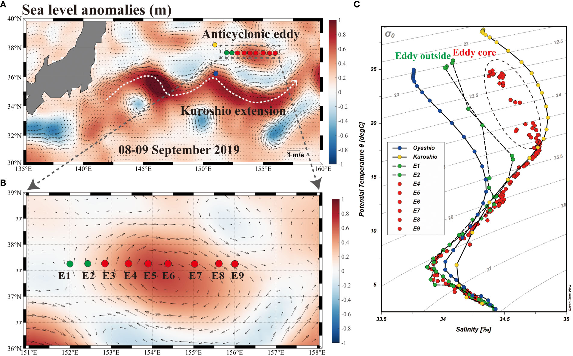
Figure 1 (A) Location of the anticyclonic eddy (dash box) in the Northern Pacific during September 8-9, 2019. Contour plots of sea level anomalies (SLA, unit:m; 0.25° resolution) were downloaded from the Copernicus Marine Environment Monitoring Service. (B) Study sites from E1 to E9. (C) Profiles of temperature vs salinity for sites E1-E9. Note that the data of temperature and salinity from 5-1000 m for the Oyashio and Kuroshio water masses were downloaded from CEMES for reference.

FIGURE 2

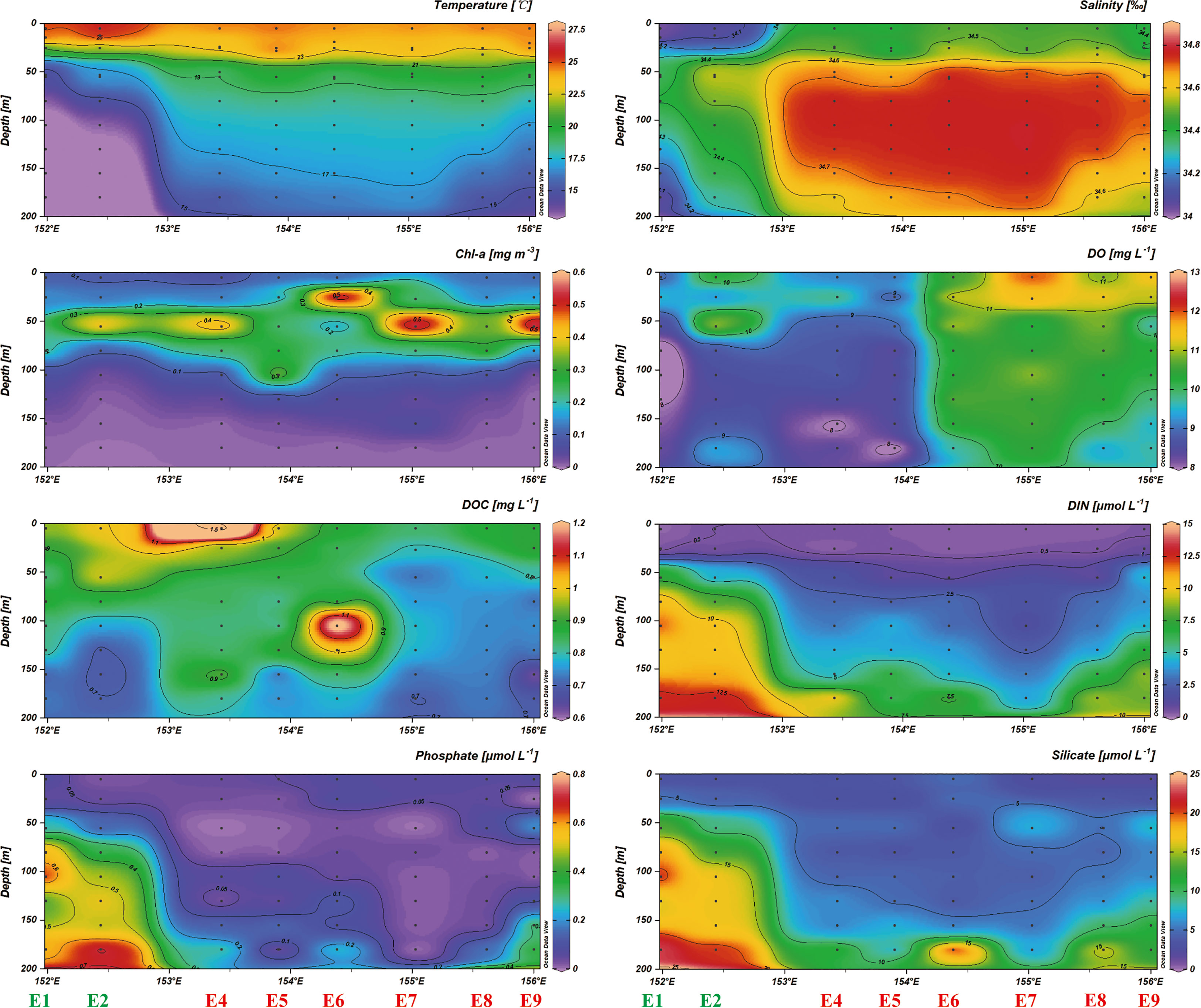
Figure 2 The vertical distribution of temperature, salinity, Chl-a, DO, DOC, DIN, phosphate, silicate in the anticyclonic eddy.

2.2 Sample collection

Water samples above 250 m were collected at sites E1 to E9 during the expedition (Figure 1). The temperature and salinity of seawater were obtained from an SBE 911 plus conductivity–temperature–depth (CTD) probe. The MLD was defined by the threshold value of temperature (0.2 °C) from the surface value at 10 m depth (de Boyer Montégut et al., 2004). Seawater samples for CH₄ and NMHCs analysis were collected from 12 L Niskin bottles. Subsamples were gently introduced into 120 mL brown glass bottles through a rubber tube and overflowed 3 times of the bottle volume, and then 50 μL saturated HgCl₂ solution was added to inhibit biological activities. Samples were then sealed with aluminum caps containing Teflon septa and temporarily stored at 4 °C in the dark (Wu et al., 2021; Li et al., 2022). About 1 L seawater was filtered through Whatman filter (0.7 μm) for chlorophyll a (Chl-a) measurement and filters were frozen at -20 °C. For the analysis of single phytoplankton cells, 50 mL seawater at sites E1, E5, and E9 was preserved in acidic Lugol’s solution at a volumetric ratio of 1:100. For the nutrients sample, ~60 mL seawater was filtered through 0.45 μm cellulose acetate filters and the filtrates were stored frozen at -20 °C. Dissolved organic carbon (DOC) samples were filtered using precombusted (450 °C, 3 hours) 0.7 μm GFF filters. All DOC samples were preserved in precombusted glass bottles with acid cleaned (10% HCl) and frozen at -20 °C until analysis. Furthermore, air samples for determining atmospheric concentrations of methane and NMHCs from three sites (E1, E4, E9) were collected in 3 L fused-silica lined stainless-steel canister (Restek, USA) from 10 m above the sea surface.

2.3 Biogeochemical analyses

Seawater CH₄ concentration was determined using a cryogenic purge and trap system connected to a gas chromatograph with a flame ionization detector (GC, Agilent 8090, USA). Dissolved CH₄ of seawater was purged with high-purity nitrogen gas (50 mL min^-1) and trapped at 1/8 stainless steel pipe (Porapak Q, 80-100 mesh) by liquid nitrogen. After purging for 10 minutes, methane was released from the trap loop by heating in a boiling water bath. The gaseous sample was introduced into gas chromatography equipped with the flame ionization detector and capillary column (HP-PLOT/Q, 30 m × 0.32 mm × 20 μm). The oven temperature was maintained at 90 °C, and the peak of the sample was shown in 2 minutes after sample introduction. The method detection limit for methane analysis in this study was 0.1 nmol L^-1, and the standard deviation was less than 3%.

Similarly, seawater NMHCs concentration was measured using a cryogenic purge and trap system connected to a gas chromatography-mass spectrometer (GC-MS, Agilent 7890A/5975C, USA). About 50 mL seawater was injected into the sparging chamber and purged with high-purity helium gas (50 mL min^-1) for 15 minutes. Anhydrous magnesium perchlorate (Mg(ClO₄)₂) and sodium hydroxide (NaOH) were used as desiccants to remove moisture. The GC was equipped with an Rt-Alumina Bond/KCl capillary column (30 m × 0.32 mm × 5 μm), and the temperature program was set as follows: oven temperature started at 40 °C for 6 minutes, gradually raised to 120 °C with the rate of 5 °C/min, held at 120 °C for 8 minutes, raised to 170 °C at 30 °C min^-1 and held at 170 °C for 10 minutes. The detection limit of the method was 0.5 pmol L^-1. In addition, atmosphere samples were measured using the GC-MS coupled with an atmospheric pre-concentrator (Nutech 8900DS, USA).

Dissolved oxygen (DO) was measured on board followed by the Winkler titration method (Bryan et al., 1976). The concentration of Chl-a was analyzed with a fluorescence spectrophotometer (Hitachi F-4500, Japan). Flow cytometry was used to determine the single phytoplankter cells (Chen et al., 2017). Pigments were excited with a 488 nm laser beam delivered by a 20 mW solid state laser. Each intercepted cell was characterised by five scatter and fluorescence signals, namely sideward scatter, red fluorescence (FLR; 668–734 nm), orange fluorescence (FLO; 601–668 nm) and yellow fluorescence (FLY, 536–601 nm). The flow cytometer was driven by the CytoSub software and data was analyzed using CytoClus3 software (CytoBuoy). Three sizes of phytoplankton community, namely picophytoplankton, nanophytoplankton and microphytoplankton were determined at sites E1, E5, and E9. The concentration of dissolved inorganic nitrogen (DIN, nitrate plus nitrite), phosphate (PO₄^3-), and silicate (SiO₃^2-) were determined with an AA3 nutrients analyzer (SEAL Analytical, UK). Samples for DOC were analyzed via the high-temperature catalytic oxidation method (Guo et al., 2011). ~10 mL sample was acidified to pH 2-3 with 2 mol L^-1 HCl, and bubbled with high-purity nitrogen (N₂) gas to remove dissolved inorganic carbon. Organic carbon was catalytically oxidized to CO₂ (with 0.5% Pt-Al₂O₃) at 680 °C, which was measured with a non-dispersive infrared gas analyzer (Shimadzu TOC-VCPH, Shimadzu Co., Japan).

2.4 Underway observation

The underway observation of pCO₂ was carried out from 152.0° E to 156.0° E along the transect of 37.6° N. Seawater at approximately 3 m below the sea surface was pumped into the laboratory and the flow rate of seawater was set to 1 L min^-1. After separation of gaseous and aqueous phase using a spraying equilibrator, gaseous samples were filtered through a 0.1 μm filter membrane before analysis using a Gas Concentration Analyzer (Picarro G2131-i, USA) with the cavity ring-down spectroscopy (CRDS). Air samples were collected from 10 m above the sea surface at the flow rate of 300 mL min^-1. The instrument was calibrated with standard gas at CO₂ levels of 200 ppmv, 400 ppmv and 600 ppmv every 3 hours (China National Research Center for Certificated Reference Materials) with an uncertainty is less than 0.1%. Sea surface temperature (SST), salinity (SSS), and Chl-a were measured by Ferrybox (4H-JENA, Germany), a highly integrated, automatic device equipped with multiple probes (SBE45, USA; Seapoint Chlorophyll Fluorometer, USA).

2.5 Nutrients transport fluxes

Nutrient flux (N_flux), representing the vertical diffusive flux of nitrate through the base of the euphotic zone, was calculated using Fick’s first law of diffusion as Eq. 1 (Shih et al., 2020).

$\begin{array}{ll}{N}_{flux}=K_z{d}_N/d_Z& \text{(Eq. 1)}\end{array}$

In Eq. 1, K_z was the average diffusion coefficient in the upper 150 m water column and d_N/d_z was the vertical gradient of nitrate between the MLD and 150 m. The diffusion coefficient was estimated using Eq. 2:

$\begin{array}{ll}{K}_z=0.25ϵn^2& \text{(Eq. 2)}\end{array}$

where ϵ represented the turbulent energy dissipation rate and was determined by the techniques outlined by Dillon (1982) and n was the buoyancy frequency, which was calculated as the vertical density gradient between the MLD and 150 m. In addition, water column inventories of N(I-N), P (I-P), and Si (I-Si) were calculated by the trapezoidal integration for the upper 150 m.

In the interior of the ocean, the biogeochemical cycle of nitrate and phosphate is affected by physical transport and the process of nitrification and denitrification, which will affect the growth of phytoplankton. N* and P* as a tracer indicating the perturbation of phytoplankton growth was calculated by Eq. 3 and Eq. 4 based on the Redfield ratio (Gruber and Sarmiento, 1997).

$\begin{array}{ll}{N}^{*}=(N-16P+2.9)*0.87& \text{(Eq. 3)}\end{array}$

$\begin{array}{ll}{P}^{*}=P-N/16& \text{(Eq. 4)}\end{array}$

In Eq. 3 and Eq. 4, N and P represent the concentration of inorganic nitrogen (nitrite + nitrate + ammonium) and phosphate, respectively. N* or P* value near zero reflects nutrient conditions approximately equal to the Redfield ratio, whereas positive and negative values of N* or P* were associated with non-conservative behavior.

2.6 Air-sea gas flux calculations

The air-sea fluxes of CO₂ (unit: g C m^-2 y^-1), methane and NMHCs (unit: mol m^-2 day^-1) was calculated with following equation (Eq. 5):

$\begin{array}{ll}F=k*({[C_{sea}]-[C_{atm}]}_{eq})& \text{(Eq. 5)}\end{array}$

where C_sea and C_atm were the concentration of hydrocarbons in the surface seawater (unit: mol L^-1) and atmosphere (unit: ppm), respectively. k, the gas transfer velocity, calculated by the empirical formula proposed by Wanninkhof (1992) as Eq. 6.

$\begin{array}{ll}k=0.251u^2{(Sc/660)}^{-0.5}& \text{(Eq. 6)}\end{array}$

where Sc was the Schmidt number in seawater, and u was the wind speed at 10 m height (unit: m s^-1).

3 Results

3.1 Physical and biogeochemical property

The temperature-salinity (T-S) diagrams of sites E1 and E2 reflect the rapid change of temperature and salinity in the water column above 50 m (Figure 1C). In contrast, the sampling sites at the eddy core generated a T-S diagram representing the more stratified water column, and an obvious feature in the isothermal curve and isohaline curve occurred at the eddy core (Figure 2). Additionally, the SST decreased from 26.7 °C to 25.2 °C and SSS varied from 34.2 to 34.6 between sites E3 and E7 (Figure 3). Across all sampling sites, the MLD ranged from 10.9 m to 30.1 m with the shallowest at the site E2 and the maximum of MLD at the edge of eddy (site E8) (Table 1).

FIGURE 3

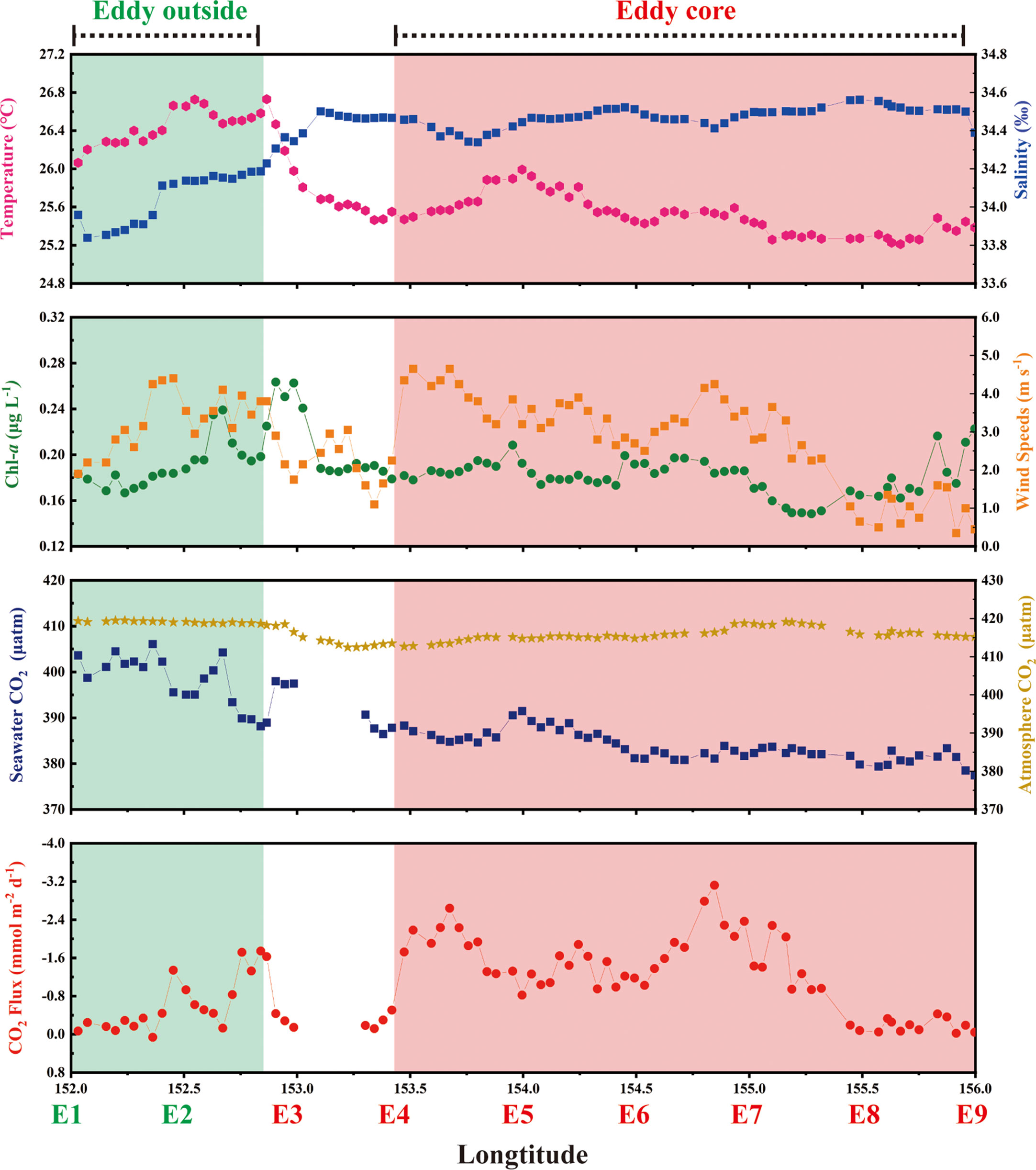
Figure 3 The underway observation of SST, SSS, Chl-a, wind speeds, [CO₂] in seawater, [CO₂] in the atmosphere, and air-sea fluxes of CO₂ at the 37.63°N transect. Noted that shadowed region represent the eddy outside (green) and core (pink).

TABLE 1

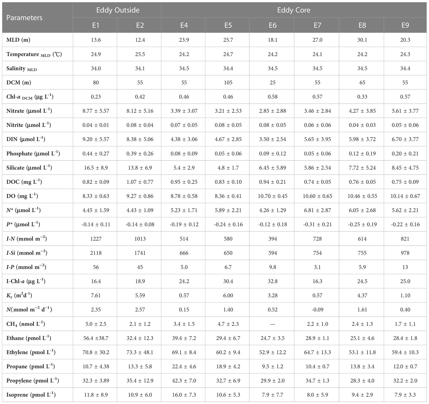
Table 1 Summary of environmental variables, including the mixed layer depth (MLD), temperature, and salinity at MLD; the maximum value of Chl-a and its depth (DCM); the average concentration of nitrate, nitrite, DIN, phosphate, silicate, dissolved organic carbon (DOC), and dissolved oxygen (DO), respectively; the abnormal of Redfield ratio for N* and P*; water column inventories (0–150 m) of DIN, silicate, phosphate, and Chl-a for I-N, I-Si, I-P, and I-Chl-a; the calculated values of diffusion coefficient (K_z); the vertical flux of N; the average concentration of methane, ethane, ethylene, propane, propylene, and isoprene, respectively.

We measured biogeochemical parameters along with nutrient distributions between the eddy outside and eddy core (Table 1). The distribution of nitrate and phosphate showed a remarkable difference between the eddy outside (nitrate, 8.43 ± 5.37 μmol L^-1; phosphate, 0.41 ± 0.27 μmol L^-1) and eddy core (nitrate, 4.03 ± 3.33 μmol L^-1; phosphate, 0.11 ± 0.15 μmol L^-1). N_flux was higher at the eddy outside (2.46 ± 0.11 mmol m⁻² d⁻¹) than at the eddy core (0.67 ± 0.63 mmol m⁻² d⁻¹). Phytoplankton biomass might also vary following the change of nutrient distribution. The range of Chl-a at the DCM for the eddy outside and inner were 0.33 ± 0.10 μg L^-1 and 0.50 ± 0.09 μg L^-1, respectively. The deep chlorophyll maximum (DCM) was considerably deepened at site E5 (80 m) corresponding to elevated DOC concentrations below the MLD (Figure 2). DOC concentration below MLD at the eddy core ranged from 0.59 to 1.42 mg L^-1 with a maximum value at 105 m depth for site E6. Furthermore, Synechococcus was the dominant species at site E1, followed by picoeukaryotes, while dominant species switched to Prochlorococcus at the eddy core. The growth of microeukaryotes and nanoeukaryotes was largely inhibited and contributed to less than 0.9%~2.4% of phytoplankton community (Figure 4).

FIGURE 4

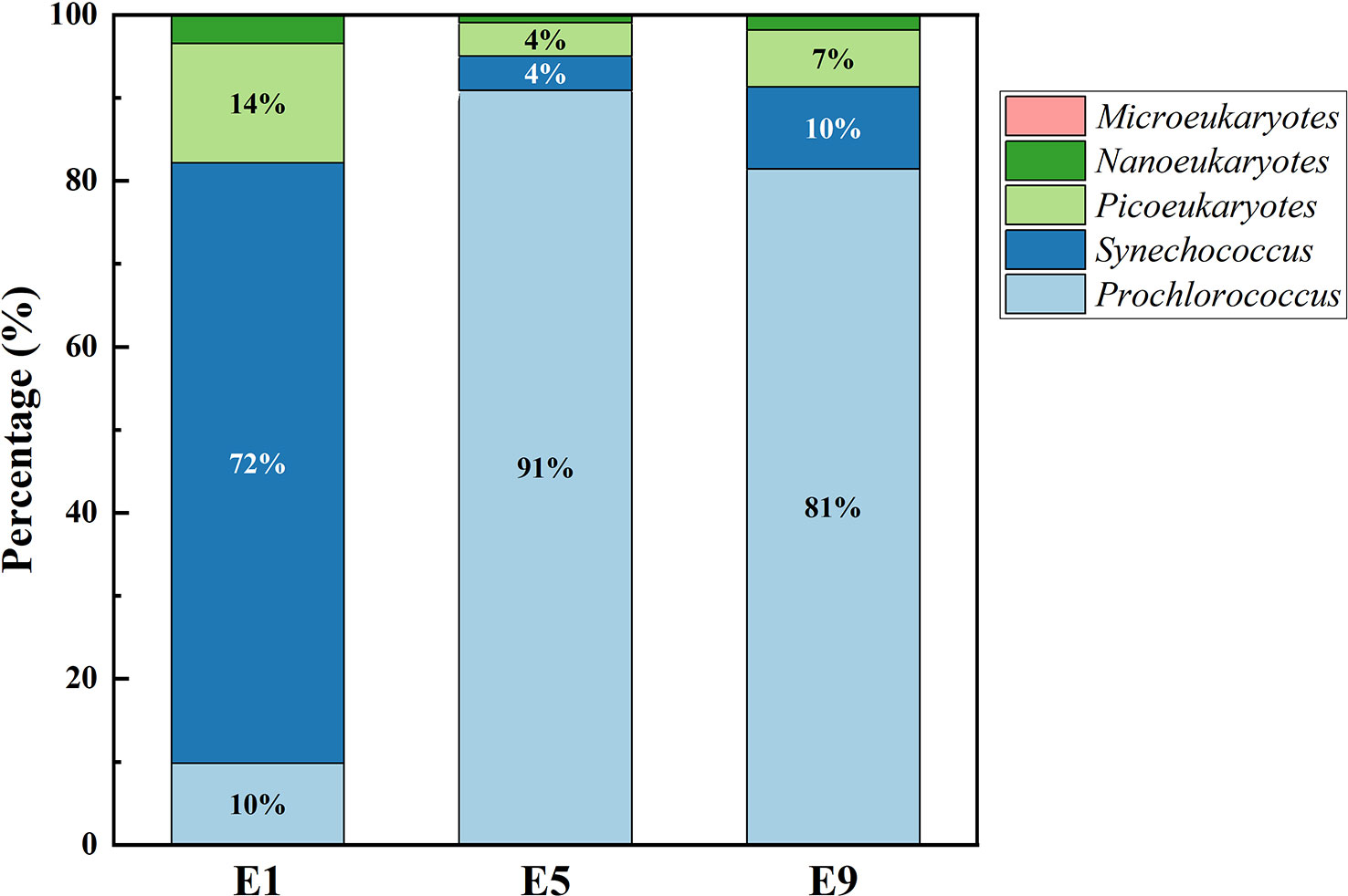
Figure 4 The proportion of the phytoplankton community in the DCM layer at the eddy outside (site E1), core (sites E5, E9).

3.2 Spatial distributions of methane and NMHCs

The change in dissolved CO₂ was similar to that of the SST, decreasing from 406.1 μatm at the eddy outside to 377.5 μatm at the eddy core (Figure 3). Across all sites, dissolved CH₄ concentrations ranged from 0.3 nmol L^-1 to 9.9 nmol L^-1, with an average of 3.4 ± 2.2 nmol L^-1. The maximum of CH₄ was observed at 80 m at the eddy core (site E05; Figure 5). At the sites E7-E9, CH₄ concentrations were< 4 nmol L^-1 and did not vary substantially with depth. Average concentrations of ethane, ethylene, propane, and propylene were 33.4 ± 18.3, 62.9 ± 22.8, 14.1 ± 5.6, 33.5 ± 7.3 pmol L^-1, respectively. Similar distributions of light alkanes and alkenes (C2-C3) were observed at site E2, and abundant hydrocarbons occurred at the surface layer and 180 m (Figure 5). Higher NMHCs concentrations were observed at the eddy core, with the maximum concentrations observed at site E4. Similar to methane, dissolved ethane, propane, and propene did not vary with depth at the sites E7-E9. In contrast, ethylene concentrations were elevated up to ~85 pmol L^-1 at site E7. Isoprene, commonly produced by phytoplankton, ranged from 3.5 pmol L^-1 to 27.9 pmol L^-1, with an average of 10.4 ± 6.7 pmol L^-1. The spatial distribution of isoprene closely matched that of Chl-a concentration with the maximum located above DCM.

FIGURE 5

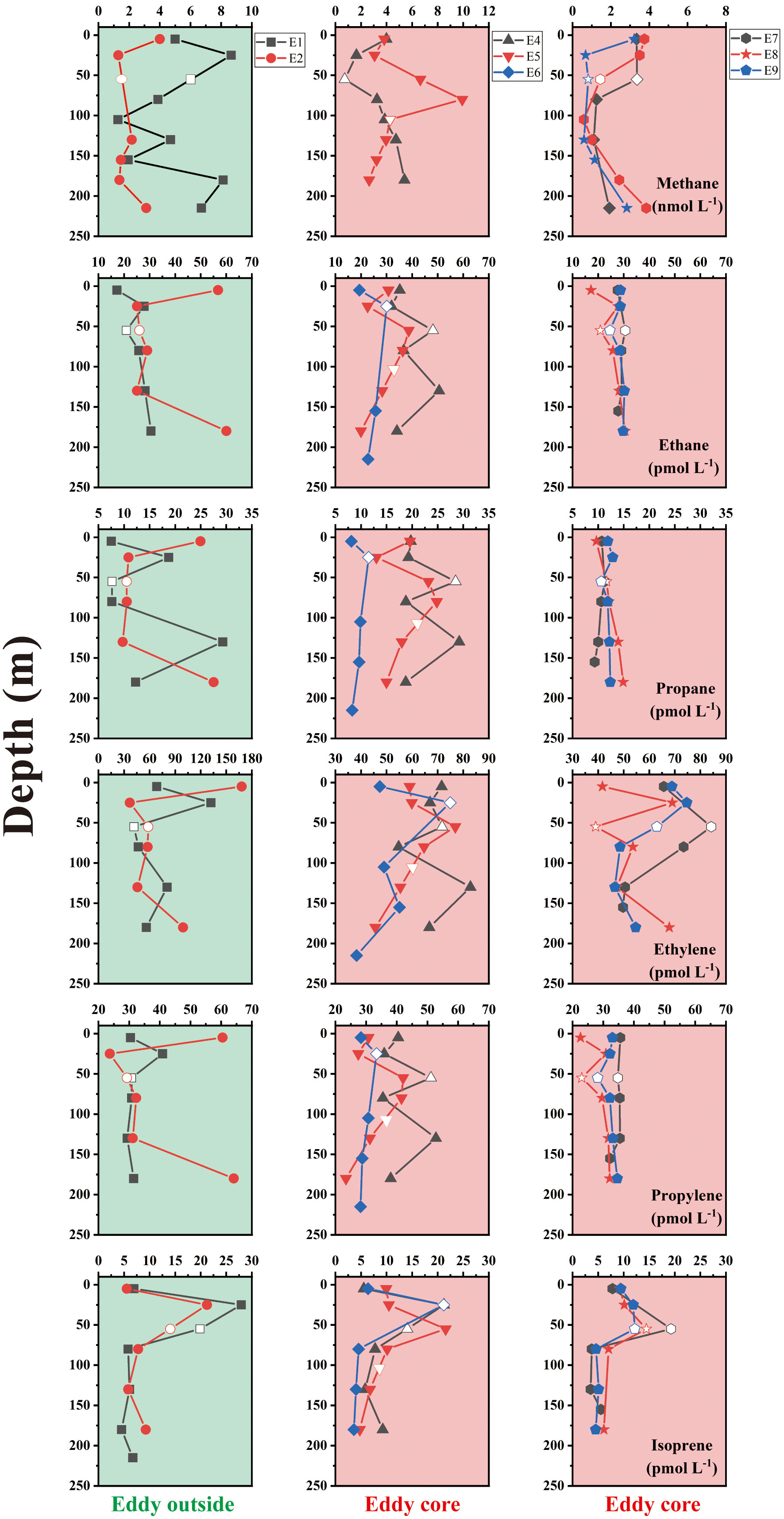
Figure 5 The vertical distribution of methane and five NMHCs (ethane, propane, ethylene, propylene, and isoprene) in the anticyclonic eddy. Note that the blank data points without color filled indicated the depth of DCM.

3.3 Air-sea fluxes of CO₂, methane and NMHCs

We compared air-sea fluxes of CO₂, methane, and NMHCs throughout the eddy to elucidate the influence of the eddy on the distribution of these compounds (Figures 3, 6). Wind speed was elevated at the eddy core sites and ranged from 1.10 to 4.65 m s^-1 with an average of 3.21 ± 0.81 m s^-1. The maximum wind speed was observed at site E4 (4.65 m s^-1). In contrast, wind speed decreased to 0.35 m s^-1 at the site E9. Air-sea fluxes of CO₂ across the eddy varied from -3.1 to 0.06 mmol m^-2 d^-1, with the maximum value calculated at the eddy core (Figure 3). Note that the negative value indicates that the ocean is a sink for the atmosphere, while the positive value represents that the ocean is a source. The air-sea fluxes of CH₄ ranged from 0.1-1.6 μmol m^-2 d^-l and was substantially lower at the sites E8-E9 relative to the other sites (Figure 6). The calculated air-sea fluxes of the five NMHCs varied from 0.9-34.7 (ethane), 2.3-108.3 (ethylene), 0.5-14.0 (propane), 1.2-34.7 (propylene), and 0.4-5.8 nmol m^-2 d^-l (isoprene), respectively. Except for isoprene, the maximum air-sea fluxes of NMHCs occurred at site E2. Instead, the maximum isoprene (4.2 ± 1.2 nmol m^-2 d^-1) fluxes were observed at the eddy core (site E5).

FIGURE 6

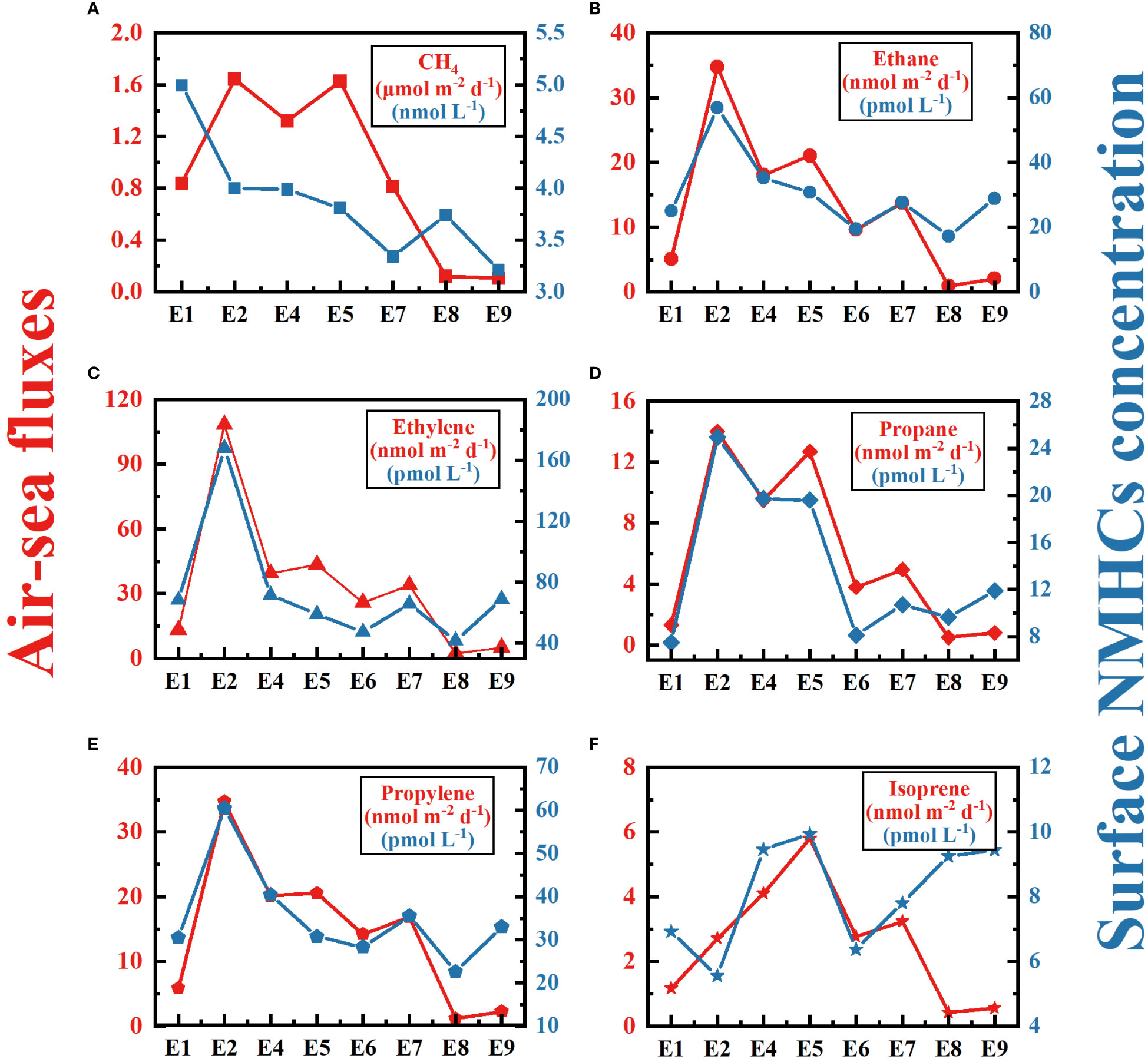
Figure 6 Surface seawater concentration (blue symbol and line) and air-sea fluxes (red symbol and line) of methane (A) and five NMHCs (E–F) at sites E1 to E9.

4 Discussion

4.1 Nutrients dynamic influenced by anticyclonic eddy

Eddy and other mesoscale processes (lateral advection, eddy pumping and eddy-driven stratification) are prevalent in the ocean and influence the distributions of nutrients and organic carbon in the upper water column (Mcgillicuddy, 2016; Shih et al., 2020). The maximum value of N fluxes at the eddy outside manifests the nutrient supplement of the deep water (Table 1), which is consistent with previous studies of nutrient enrichment at the edge of anticyclonic eddies (Zhou et al., 2013; Mcgillicuddy, 2016). Likewise, the value of I-N, I-P and I-Si were higher at the eddy outside compared to other sites in the eddy system (Table 1). Therefore, the upper water column of the eddy core represents a nutrient limitation compared to the eddy outside.

Furthermore, N* increased from 4.44 ± 1.35 μmol kg^-1 (eddy outside) to 5.71 ± 2.35 μmol kg^-1 (eddy core). Phosphate concentrations were limited as reflected by a decrease in P* (-0.14 ~ -0.26). The limitation of nutrients will restrict the development of phytoplankton in the anticyclonic eddy. In our study, large size eukaryotes such as nanophytoplankton and microphytoplankton were detected with low abundance, but Prochlorococcus was highly abundant at the eddy core. In addition, elevated phytoplankton cell mortality rates and cell lysis rates at the anticyclonic eddy could be responsible for the higher DOC production (Lasternas et al., 2013). Taken together, the process of anticyclonic eddy leads to a change in nutrient conditions, phytoplankton structure in the upper ocean.

4.2 Potential controlling factors of methane and NMHCs in the eddy

Methane production is directly linked to the N, P and C cycles as feedback of environmental perturbations such as changes in phytoplankton structure and nutrient supply (Damm et al., 2008; Karl et al., 2008). The methane maximum at site E5 in the eddy outside may be related to the low nutrient level in the water column (Weller et al., 2013). Under nutrient limited conditions, microorganisms can use compounds such as methylamine and methylphosphonate (MPn) as alternative sources of P and N (Repeta et al., 2016; Ye et al., 2020; Mao et al., 2022). The microbial utilization of MPn lead to the lyase of C-P and CH₄ could be produced as a by-product (Repeta et al., 2016; Acker et al., 2022). Furthermore, most semi-labile DOM including MPn is produced by Prochlorococcus in the open ocean (Repeta et al., 2016). Hence, the growth of Prochlorococcus at the eddy core facilitated methane production through the C-P pathway. The vertical distribution of methane is homogenous at sites E7 and E8, which could be caused by the increasing depth of the mixing layer.

Isoprene is produced biologically by phytoplankton, and its distribution reflects the abundance and structure of phytoplankton (Broadgate et al., 2004; Li et al., 2019; Conte et al., 2020). As such, a subsurface maximum was observed for the concentration of isoprene in the water column, generally consistent with the depth of DCM (Figure 5). Interestingly, strong correlation between the isoprene and Chl-a was observed at the eddy core (R²=0.38; n=32; P<0.01), while little correlation occurred at the eddy outside (R²=0.003; n=11; P>0.01). Such difference indicated that phytoplankton structure could be important in the isoprene distribution as the production of isoprene was species-dependent (Broadgate et al., 1997; Kurihara et al., 2010; Li et al., 2021). It has been demonstrated that Prochlorococcus was an important producer of isoprene in the open ocean (Shaw et al., 2003). At the eddy core, the abundance of Prochlorococcus was much higher than other species, suggesting that Prochlorococcus dominate the production of isoprene and also explained the observed correlation between isoprene and Chl-a. Previous laboratory studies have found various species of microeukaryotes, nanoeukaryotes, picoeukaryotes and cyanobacteria (including Prochlorococcus and Synechococcus) are all the isoprene producers (McKay et al., 1996; Shaw et al., 2003). Although the size of the phytoplankton cell influences the production rate, the abundance of Prorochlorococcus is one or two orders of magnitude higher than that of other eukaryotes. Therefore, the succession of small-size phytoplankton leads to the variation of isoprene in the anticyclonic eddy. In contrast to isoprene, other NMHCs have different sources, and the distribution could be impacted by other environmental factors. Previous studies found light NMHCs can be produced through the degradation of polyunsaturated lipids, which originate from marine phytoplankton (Lee and Baker, 1992; Broadgate et al., 2004; Plettner et al., 2005). The concentrations of ethane and ethylene at the eddy outside were higher than those at the eddy core, in which the abundant DOC was enriched at the surface layer. The maximum of NMHCs occurred near DCM at the sites E5 and E6, which could be caused by the degradation of phytoplankton-related organic matter. Similar to methane, ethylene and propylene can also be produced by the bacterial degradation of phosphonates (Repeta et al., 2016). Increased phytoplankton mortality during the eddy process would enhance the autolysis of phytoplankton cells, which could contribute to the subsurface maximum for ethane and propane (McKay et al., 1996). Principal component analysis (PCA) is used to analyze the influence of environmental factors on methane and NMHCs in eddy process (Figure 7). The results of PCA analysis illustrate that two principal components explain >60% of the total variation. For Figures 7A, B, PC1 is related to the temperature and nutrients (DIN, phosphate, silicate) and PC2 is significantly loaded by salinity, DOC. Methane exerts major contribution to PC2, indicating that the spatial distribution of DOC influenced by eddy activity affects the methane production, such as MPn pathway. By contrast, isoprene was strongly loaded in the PC2, illustratate that isoprene may be more sensitive to temperature. Previous studies with phytoplankton monocultures have found positive dependence of isoprene production rate on temperature within -0.8 ~ 23 °C, which is restricted to the enzymatic activities (Shaw et al., 2003; Simó et al., 2022). Our results also indicated 23 °C is the optimum temperature for isoprene production (R²=0.286; n=34; P<0.01; Figure S2), which is responsible for the maximum value at the subsurface (Simó et al., 2022). In addition, the response of light alkanes and alkenes to environmental factors may be complicated, especially the biological factors are relatively weak (Figure 7C). Furthermore, the strong correlation was observed between light alkanes and alkenes, which suggested that similar source or removal processes was affected by eddy activity (Figure 7D).

FIGURE 7

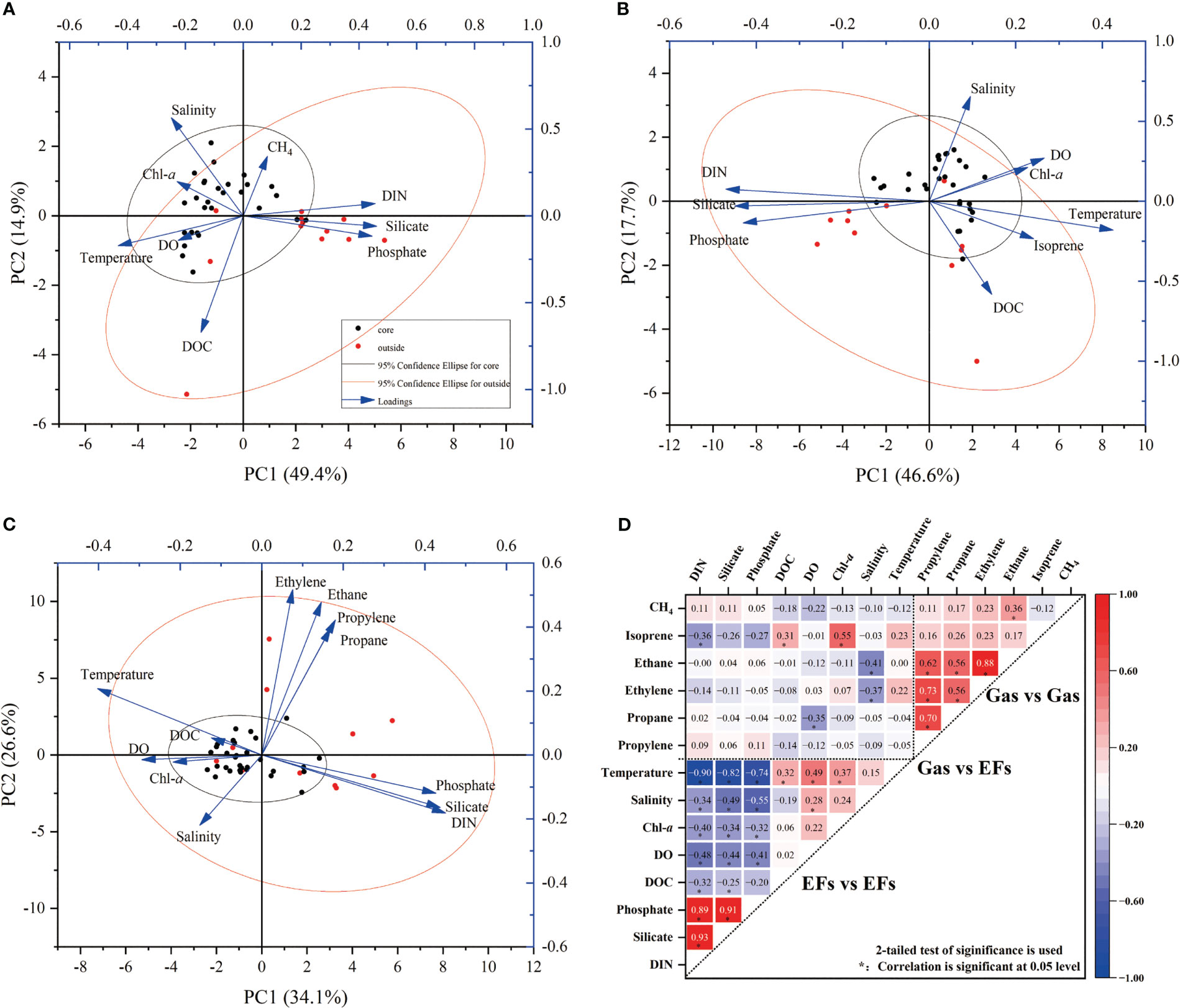
Figure 7 Principal component analysis (PCA, A–C) and correlation analysis (D) of methane, NMHCs and environmental factors. For (A–C), the red dot represents the eddy outside station (E1,E2), the black dot represents the eddy core station (E4-E9); 95% confidence was marked by ellipse; the blue arrow indicates the variables used for PCA, and the percentage of variance is displayed on the x and y axis. For (D), Pearson’s correlation coefficient is used for correlation analysis; the asterisk (*) indicates a correlation coefficient of less than 0.05 level.

4.3 Effect of anticyclone eddy on the air-sea fluxes of gases

The occurrence of ocean eddies exerts curial influence on the vertical structure of the marine atmospheric boundary layer and further affects many atmospheric processes including air turbulence, wind speeds, as well as air-sea exchange (Frenger et al., 2013; Weller et al., 2013; Pezzi et al., 2021). Apparently, the sites E2-E7 were influenced by a strong wind field (2.93-3.47 m s^-1), while the wind speed at the sites E1 (1.88 m s^-1), E8 (0.97 m s^-1) and E9 (1.11 m s^-1) were relatively calm. For air-sea exchange, the calculated air-sea fluxes of CO₂ in this anticyclone eddy (-1.04 ± 0.80 mmol m^-2 d^-1) were lower than those reported values in the KOE region (-6.5 mmol m^-2 d^-1, Sutton et al., 2017; -2.70 ± 2.31 mmol m^-2 d^-1, Yan et al., 2023) and North Pacific extratropic (2.42 ± 0.67 mmol m^-2 d^-1, Ishii et al., 2014). In addition, the sink of CO₂ at the eddy core (-1.27 ± 0.78 mmol m^-2 d^-1) was stronger than the eddy outside (-0.60 ± 0.57 mmol m^-2 d^-1). According to Eq. 5 and Eq. 6, the elevated air-sea CO₂ exchange at the eddy core could be joint result of lower SST, higher pCO₂, and strong winds. Furthermore, air-sea fluxes for methane (0.10-1.64 μmol m^-2 d^-1) and isoprene (0.42-5.79 nmol m^-2 d^-1) were lower than the reported values in the Pacific (methane: 1.64-2.93 μmol m^-2 d^-1, Rehder and Suess, 2001; Isoprene: 2.1-300 nmol m^-2 d^-1, Matsunaga et al., 2002; Li et al., 2019). Higher methane emission occurred at sites E2 and E5, and the maximum flux of isoprene occurred at site E5 where had the highest surface concentration. For other NMHCs, the emissions of ethane, ethylene, and propylene appear to be attenuated at the site E6-E9 due to the decrease in surface concentration. Collectively, eddy processes can affect local regional sea-air exchange processes by influencing water temperature, gas concentrations and wind fields. Globally, the effect of eddy on gas emissions could be important given the prevalence of mesoscale eddies in the ocean, which should be considered in the estimation of global sea-air fluxes in the future.

5 Summary

In this study, we investigate the distribution and emission of climate-relevant gases including CO₂, methane, and NMHCs in an anticyclone eddy in the KOE during September 8-9, 2019. The eddy exhibited remarkable nutrient limitation due to the downward isopycnal displacement, which favored the growth of small-size phytoplankton, especially Prochlorococcus. Phosphorus limitation within the eddy facilitated the production of methane from the C-P pathway. Significant correlation was observed between dissolved isoprene and Chl-a due to the dominance of Prochlorococcus at the eddy core sites. The elevated concentrations of ethane, propane, ethylene, and propylene in the water column could be related to the production of DOC. Air-sea fluxes of gases were largely influenced by the anticyclone mesoscale eddy. The ventilation of CO₂ and isoprene increased at the eddy core, while the air-sea fluxes of methane and light NMHCs were lower at the eddy outside due to the reduced wind speeds. Our results indicate mesoscale eddy exerts an important influence on the distribution and emission of light hydrocarbons, short-lived ocean events such as mesoscale eddies should be considered in the future estimates of gas fluxes.

Data availability statement

The original contributions presented in the study are included in the article/Supplementary Material. Further inquiries can be directed to the corresponding authors.

Author contributions

H-HZ and G-CZ designed the study. X-JL performed the experiments, with assistance from JW, and HQ. JW provided NMHCs data and HQ provided DO data. Phytoplankton data was provided by SZ. X-JL organized and analyzed the database, wrote the manuscript and prepared the tables and figures. H-HZ, AM, G-CZ, Z-HC, and R-CZ provided comments on data analysis and revised the manuscript. All authors contributed to the article and approved the submitted version.

Funding

This work was financially supported by the National Natural Science Foundation of China (Nos. 42276042; 42076031); the Fundamental Research Funds for the Central Universities (Nos. 202161060; 202072001); the Taishan Scholars Program of Shandong Province (No. tsqn201909057; G.-C. Zhuang); Laoshan Laboratory (No. LSKJ202201701), the National Key Research and Development Program of China (No. 2022YFE0136300).

Acknowledgments

We thank the chief scientist, captain and crews of the R/V ‘Dong Fang Hong 3’ for assistance and cooperation during the investigation.

Conflict of interest

The authors declare that the research was conducted in the absence of any commercial or financial relationships that could be construed as a potential conflict of interest.

Publisher’s note

All claims expressed in this article are solely those of the authors and do not necessarily represent those of their affiliated organizations, or those of the publisher, the editors and the reviewers. Any product that may be evaluated in this article, or claim that may be made by its manufacturer, is not guaranteed or endorsed by the publisher.

Supplementary material

The Supplementary Material for this article can be found online at: https://www.frontiersin.org/articles/10.3389/fmars.2023.1181896/full#supplementary-material

References

Acker M., Hogle S. L., Berube P. M., Hackl T., Coe A., Stepanauskas R., et al. (2022). Phosphonate production by marine microbes: exploring new sources and potential function. Proc. Natl. Acad. Sci. 119 (11), e2113386119. doi: 10.1073/pnas.2113386119

CrossRef Full Text | Google Scholar

Atkinson R. (2000). Atmospheric chemistry of VOCs and NOx. Atmospheric Environ. 34 (12), 2063–2101. doi: 10.1016/S1352-2310(99)00460-4

CrossRef Full Text | Google Scholar

Borges A. V., Champenois W., Gypens N., Delille B., Harlay J. (2016). Massive marine methane emissions from near-shore shallow coastal areas. Sci. Rep. 6 (1), 27908. doi: 10.1038/srep27908

PubMed Abstract | CrossRef Full Text | Google Scholar

Bourtsoukidis E., Pozzer A., Sattler T., Matthaios V. N., Ernle L., Edtbauer A., et al. (2020). The red Sea deep water is a potent source of atmospheric ethane and propane. Nat. Commun. 11 (1), 447. doi: 10.1038/s41467-020-14375-0

PubMed Abstract | CrossRef Full Text | Google Scholar

Broadgate W. J., Liss P. S., Penkett S. A. (1997). Seasonal emissions of isoprene and other reactive hydrocarbon gases from the ocean. Geophys. Res. Lett. 24 (21), 2675–2678. doi: 10.1029/97GL02736

CrossRef Full Text | Google Scholar

Broadgate W. J., Malin G., Küpper F. C., Thompson A., Liss P. S. (2004). Isoprene and other non-methane hydrocarbons from seaweeds: a source of reactive hydrocarbons to the atmosphere. Mar. Chem. 88 (1), 61–73. doi: 10.1016/j.marchem.2004.03.002

CrossRef Full Text | Google Scholar

Bryan J. R., Rlley J. P., Williams P. J. L. (1976). A winkler procedure for making precise measurements of oxygen concentration for productivity and related studies. J. Exp. Mar. Biol. Ecol. 21 (3), 191–197. doi: 10.1016/0022-0981(76)90114-3

CrossRef Full Text | Google Scholar

Chen Y., Sun X., Zhu M., Zheng S., Yuan Y., Denis M. (2017). Spatial variability of phytoplankton in the pacific western boundary currents during summer 2014. Mar. Freshw. Res. 68 (10), 1887–1900. doi: 10.1071/MF16297

CrossRef Full Text | Google Scholar

Conte L., Szopa S., Aumont O., Gros V., Bopp L. (2020). Sources and sinks of isoprene in the global open ocean: simulated patterns and emissions to the atmosphere. J. Geophysical Research: Oceans 125 (9), e2019JC015946. doi: 10.1029/2019JC015946

CrossRef Full Text | Google Scholar

Damm E., Kiene R. P., Schwarz J., Falck E., Dieckmann G. (2008). Methane cycling in Arctic shelf water and its relationship with phytoplankton biomass and DMSP. Mar. Chem. 109 (1), 45–59. doi: 10.1016/j.marchem.2007.12.003

CrossRef Full Text | Google Scholar

de Boyer Montégut C., Madec G., Fischer A. S., Lazar A., Iudicone D. (2004). Mixed layer depth over the global ocean: an examination of profile data and a profile-based climatology. J. Geophysical Research: Oceans 109 (C12). doi: 10.1029/2004JC002378

CrossRef Full Text | Google Scholar

Dillon T. M. (1982). Vertical overturns: a comparison of Thorpe and ozmidov length scales. J. Geophysical Research: Oceans 87 (C12), 9601–9613. doi: 10.1029/JC087iC12p09601

CrossRef Full Text | Google Scholar

Exton D. A., McGenity T. J., Steinke M., Smith D. J., Suggett D. J. (2015). Uncovering the volatile nature of tropical coastal marine ecosystems in a changing world. Global Change Biol. 21 (4), 1383–1394. doi: 10.1111/gcb.12764

CrossRef Full Text | Google Scholar

Faghmous J. H., Frenger I., Yao Y., Warmka R., Lindell A., Kumar V. (2015). A daily global mesoscale ocean eddy dataset from satellite altimetry. Sci. Data 2 (1), 150028. doi: 10.1038/sdata.2015.28

PubMed Abstract | CrossRef Full Text | Google Scholar

Farias L., Troncoso M., Sanzana K., Verdugo J., Italo M. (2021). Spatial distribution of dissolved methane over extreme oceanographic gradients in the subtropical Eastern south pacific (17° to 37°S). J. Geophysical Research: Oceans 126 (5), e2020JC016925. doi: 10.1029/2020JC016925

CrossRef Full Text | Google Scholar

Frenger I., Gruber N., Knutti R., Münnich M. (2013). Imprint of southern ocean eddies on winds, clouds and rainfall. Nat. Geosci. 6 (8), 608–612. doi: 10.1038/ngeo1863

CrossRef Full Text | Google Scholar

Gaube P., McGillicuddy J. Jr., D. and Moulin A. J. (2019). Mesoscale eddies modulate mixed layer depth globally. Geophysical Res. Lett. 46 (3), 1505–1512. doi: 10.1029/2018GL080006

CrossRef Full Text | Google Scholar

Gruber N., Sarmiento J. L. (1997). Global patterns of marine nitrogen fixation and denitrification. Glob. Biogeochem. Cycles 11 (2), 235–266. doi: 10.1029/97GB00077

CrossRef Full Text | Google Scholar

Guo W. D., Yang L. Y., Hong H. S., Stedmon C. A., Wang F. L., Xu J., et al. (2011). Assessing the dynamics of chromophoric dissolved organic matter in a subtropical estuary using parallel factor analysis. Mar. Chem. 124 (1), 125–133. doi: 10.1016/j.marchem.2011.01.003

CrossRef Full Text | Google Scholar

Hausmann U., McGillicuddy J. D. J., Marshall J. (2017). Observed mesoscale eddy signatures in southern ocean surface mixed-layer depth. J. Geophysical Research: Oceans 122 (1), 617–635. doi: 10.1002/2016JC012225

CrossRef Full Text | Google Scholar

IPCC (2018). “Global warming of 1.5 °C, an IPCC special report on the impacts of global warming of 1.5 °C above pre-industrial levels and related global greenhouse gas emission pathways, in the context of strengthening the global response to the threat of climate change, sustainable development, and efforts to eradicate poverty,” in Summary for policy makers. Geneva, Switzerland: IPCC Available online: http://report.ipcc.ch/sr15/pdf/sr15_spm_final.pdf.

Google Scholar

Ishii M., Feely R. A., Rodgers K. B., Park G. H., Wanninkhof R., Sasano D., et al. (2014). Air–sea CO₂ flux in the Pacific Ocean for the period 1990–2009. Biogeosciences 11 (3), 709–734. doi: 10.5194/bg-11-709-2014

CrossRef Full Text | Google Scholar

Itoh S., Yasuda I. (2010). Characteristics of mesoscale eddies in the kuroshio-oyashio extension region detected from the distribution of the Sea surface height anomaly. J. Phys. Oceanogr. 40 (5), 1018–1034. doi: 10.1175/2009JPO4265.1

CrossRef Full Text | Google Scholar

Jickells T. D., Liss P. S., Broadgate W., Turner S., Kettle A. J., Read J., et al. (2008). A Lagrangian biogeochemical study of an eddy in the northeast Atlantic. Prog. Oceanogr. 76 (3), 366–398. doi: 10.1016/j.pocean.2008.01.006

CrossRef Full Text | Google Scholar

Kansal A. (2009). Sources and reactivity of NMHCs and VOCs in the atmosphere: a review. J. Hazard. Mater. 166 (1), 17–26. doi: 10.1016/j.jhazmat.2008.11.048

PubMed Abstract | CrossRef Full Text | Google Scholar

Karl D. M., Beversdorf L., Björkman K. M., Church M. J., Martinez A., Delong E. F. (2008). Aerobic production of methane in the sea. Nat. Geosci. 1 (7), 473–478. doi: 10.1038/ngeo234

CrossRef Full Text | Google Scholar

Kurihara M. K., Kimura M., Iwamoto Y., Narita Y., Ooki A., Eum Y. J., et al. (2010). Distributions of short-lived iodocarbons and biogenic trace gases in the open ocean and atmosphere in the western north pacific. Mar. Chem. 118 (3), 156–170. doi: 10.1016/j.marchem.2009.12.001

CrossRef Full Text | Google Scholar

Lasternas S., Piedeleu M., Sangrà P., Duarte C. M., Agustí S. (2013). Forcing of dissolved organic carbon release by phytoplankton by anticyclonic mesoscale eddies in the subtropical NE Atlantic ocean. Biogeosciences 10 (3), 2129–2143. doi: 10.5194/bg-10-2129-2013

CrossRef Full Text | Google Scholar

Lee R. F., Baker J. (1992). Ethylene and ethane production in an estuarine river: formation from the decomposition of polyunsaturated fatty acids. Mar. Chem. 38 (1), 25–36. doi: 10.1016/0304-4203(92)90065-I

CrossRef Full Text | Google Scholar

Li Y., Fichot C. G., Geng L., Scarratt M. G., Xie H. (2020). The contribution of methane photoproduction to the oceanic methane paradox. Geophysical Res. Lett. 47 (14), e2020GL088362. doi: 10.1029/2020GL088362

CrossRef Full Text | Google Scholar

Li X., Liang H., Zhuang G., Wu Y., Li S., Zhang H., et al. (2022). Annual variations of isoprene and other non-methane hydrocarbons in the jiaozhou bay on the East coast of north China. J. Geophysical Research: Biogeosciences 127 (3), e2021JG006531. doi: 10.1029/2021JG006531

CrossRef Full Text | Google Scholar

Li J., Zhai X., Ma Z., Zhang H., Yang G. (2019). Spatial distributions and sea-to-air fluxes of non-methane hydrocarbons in the atmosphere and seawater of the Western pacific ocean. Sci. Total Environ. 672, 491–501. doi: 10.1016/j.scitotenv.2019.04.019

PubMed Abstract | CrossRef Full Text | Google Scholar

Li J., Zhai X., Wu Y., Wang J., Zhang H., Yang G. (2021). Emissions and potential controls of light alkenes from the marginal seas of China. Sci. Total Environ. 758, 143655. doi: 10.1016/j.scitotenv.2020.143655

PubMed Abstract | CrossRef Full Text | Google Scholar

Mao S., Zhang H., Zhuang G., Li X., Liu Q., Zhou Z., et al. (2022). Aerobic oxidation of methane significantly reduces global diffusive methane emissions from shallow marine waters. Nat. Commun. 13 (1), 7309. doi: 10.1038/s41467-022-35082-y

PubMed Abstract | CrossRef Full Text | Google Scholar

Matsunaga S., Mochida M., Saito T., Kawamura K. (2002). In situ measurement of isoprene in the marine air and surface seawater from the western north pacific. Atmospheric Environ. 36 (39), 6051–6057. doi: 10.1016/S1352-2310(02)00657-X

CrossRef Full Text | Google Scholar

Mcgillicuddy D. (2016). Mechanisms of physical-Biological-Biogeochemical interaction at the oceanic mesoscale. Annu. Rev. Mar. Sci. 8, 125–126. doi: 10.1146/annurev-marine-010814-015606

CrossRef Full Text | Google Scholar

McKay W. A., Turner M. F., Jones B. M. R., Halliwell C. M. (1996). Emissions of hydrocarbons from marine phytoplankton–some results from controlled laboratory experiments. Atmospheric Environ. 30 (14), 2583–2593. doi: 10.1016/1352-2310(95)00433-5

CrossRef Full Text | Google Scholar

Pezzi L. P., de Souza R. B., Santini M. F., Miller A. J., Carvalho J. T., Parise C. K., et al. (2021). Oceanic eddy-induced modifications to air–sea heat and CO₂ fluxes in the Brazil-malvinas confluence. Sci. Rep. 11 (1), 10648. doi: 10.1038/s41598-021-89985-9

PubMed Abstract | CrossRef Full Text | Google Scholar

Plass-Dülmer C., Koppmann R., Ratte M., Rudolph J. (1995). Light nonmethane hydrocarbons in seawater. Glob. Biogeochem. Cycles 9 (1), 79–100. doi: 10.1029/94GB02416

CrossRef Full Text | Google Scholar

Plettner I., Steinke M., Malin G. (2005). Ethylene (ethylene) production in the marine macroalga ulva (Enteromorpha) intestinalis l (Chlorophyta Ulvophyceae): effect light-stress co-production dimethyl sulphide. Plant Cell Environ. 28 (9), 1136–1145. doi: 10.1111/j.1365-3040.2005.01351.x

CrossRef Full Text | Google Scholar

Ratte M., Bujok O., Spitzy A., Rudolph J. (1998). Photochemical alkene formation in seawater from dissolved organic carbon: results from laboratory experiments. J. Geophys. Res. 103 (D5), 5707–5718. doi: 10.1029/97JD03473

CrossRef Full Text | Google Scholar

Rehder G., Suess E. (2001). Methane and pCO₂ in the kuroshio and the south China Sea during maximum summer surface temperatures. Mar. Chem. 75 (1), 89–108. doi: 10.1016/S0304-4203(01)00026-3

CrossRef Full Text | Google Scholar

Repeta D. J., Ferrón S., Sosa O. A., Johnson C. G., Repeta L. D., Acker M., et al. (2016). Marine methane paradox explained by bacterial degradation of dissolved organic matter. Nat. Geosci. 9 (12), 884–887. doi: 10.1038/ngeo2837

CrossRef Full Text | Google Scholar

Riemer D. D., Milne P. J., Zika R. G., Pos W. H. (2000). Photoproduction of nonmethane hydrocarbons (NMHCs) in seawater. Mar. Chem. 71 (3), 177–198. doi: 10.1016/S0304-4203(00)00048-7

CrossRef Full Text | Google Scholar

Rosentreter J. A., Borges A. V., Deemer B. R., Holgerson M. A., Liu S., Song C., et al. (2021). Half of global methane emissions come from highly variable aquatic ecosystem sources. Nat. Geosci. 14 (4), 225–230. doi: 10.1038/s41561-021-00715-2

CrossRef Full Text | Google Scholar

Saunois M., Jackson R., Poulter B., Canadell J. (2016). The growing role of methane in anthropogenic climate change. Environ. Res. Lett. 11 (12), 120207. doi: 10.1088/1748-9326/11/12/120207

CrossRef Full Text | Google Scholar

Shaw S. L., Chisholm S. W., Prinn R. G. (2003). Isoprene production by prochlorococcus, a marine cyanobacterium, and other phytoplankton. Mar. Chem. 80 (4), 227–245. doi: 10.1016/S0304-4203(02)00101-9

CrossRef Full Text | Google Scholar

Shih Y., Hung C., Tuo S., Shao H., Chow C. H., Muller F., et al. (2020). The impact of eddies on nutrient supply, diatom biomass and carbon export in the northern south China Sea. Front. Earth Sci. 8. doi: 10.3389/feart.2020.537332

CrossRef Full Text | Google Scholar

Simó R., Cortés-Greus P., Rodríguez-Ros P., Masdeu-Navarro M. (2022). Substantial loss of isoprene in the surface ocean due to chemical and biological consumption. Commun. Earth Environ. 3 (1), 20. doi: 10.1038/s43247-022-00352-6

CrossRef Full Text | Google Scholar

Sosa O. A., Burrell T. J., Wilson S. T., Foreman R. K., Karl D. M., Repeta D. J. (2020). Phosphonate cycling supports methane and ethylene supersaturation in the phosphate-depleted western north Atlantic ocean. Limnol. Oceanogr. 65 (10), 2443–2459. doi: 10.1002/lno.11463

CrossRef Full Text | Google Scholar

Spingys C. P., Williams R. G., Tuerena R. E., Naveira Garabato A., Vic C., Forryan A., et al. (2021). Observations of nutrient supply by mesoscale eddy stirring and small-scale turbulence in the oligotrophic north Atlantic. Glob. Biogeochem. Cycles 35 (12), e2021GB007200. doi: 10.1029/2021GB007200

CrossRef Full Text | Google Scholar

Steinle L., Graves C. A., Treude T., Ferré B., Biastoch A., Bussmann I., et al. (2015). Water column methanotrophy controlled by a rapid oceanographic switch. Nat. Geosci. 8 (5), 378–382. doi: 10.1038/ngeo2420

CrossRef Full Text | Google Scholar

Sugimoto S., Aono K., Fukui S. (2017). Local atmospheric response to warm mesoscale ocean eddies in the kuroshio–oyashio confluence region. Sci. Rep. 7 (1), 11871. doi: 10.1038/s41598-017-12206-9

PubMed Abstract | CrossRef Full Text | Google Scholar

Sutton A. J., Wanninkhof R., Sabine C. L., Feely R. A., Cronin M. F., Weller R. A. (2017). Variability and trends in surface seawater pCO₂ and CO₂ flux in the pacific ocean. Geophys. Res. Lett. 44 (11), 5627–5636. doi: 10.1002/2017GL073814

CrossRef Full Text | Google Scholar

Tozuka T., Cronin M. F., Tomita H. (2017). Surface frontogenesis by surface heat fluxes in the upstream kuroshio extension region. Sci. Rep. 7 (1), 10258. doi: 10.1038/s41598-017-10268-3

PubMed Abstract | CrossRef Full Text | Google Scholar

Wanninkhof R. (1992). Relationship between wind speed and gas exchange over the ocean. Limnology Oceanography: Methods 97 (C5), 733–7382. doi: 10.1029/92JC00188

CrossRef Full Text | Google Scholar

Weller D., Law C., Marriner A., Chang F., Stephens J., Wilhelm S., et al. (2013). Temporal variation of dissolved methane in a subtropical mesoscale eddy during a phytoplankton bloom in the southwest pacific ocean. Prog. In Oceanogr. 116, 193–206. doi: 10.1016/j.pocean.2013.07.008

CrossRef Full Text | Google Scholar

Williams R. G., Wilson C., Hughes C. W. (2007). Ocean and atmosphere storm tracks: the role of eddy vorticity forcing. J. Phys. Oceanogr. 37 (9), 2267–2289. doi: 10.1175/JPO3120.1

CrossRef Full Text | Google Scholar

Wu Y., Li J., Wang J., Zhuang G., Liu X., Zhang H., et al. (2021). Occurance, emission and environmental effects of non-methane hydrocarbons in the yellow Sea and the East China Sea. Environ. Pollut. 270, 116305. doi: 10.1016/j.envpol.2020.116305

PubMed Abstract | CrossRef Full Text | Google Scholar

Yan S., Li X., Xu F., Zhang H., Wang J., Zhang Y., et al. (2023). High-resolution distribution and emission of dimethyl sulfide and its relationship with pCO₂ in the Northwest pacific ocean. Front. Mar. Sci. 10:1074474. doi: 10.3389/fmars.2023.1074474

CrossRef Full Text | Google Scholar

Ye W., Wang X., Zhang X., Zhang G. (2020). Methane production in oxic seawater of the western north pacific and its marginal seas. Limnol. Oceanogr. 65 (10), 2352–2365. doi: 10.1002/lno.11457

CrossRef Full Text | Google Scholar

Yoshikawa C., Hayashi E., Yamada K., Yoshida O., Toyoda S., Yoshida N. (2014). Methane sources and sinks in the subtropical south pacific along 17°S as traced by stable isotope ratios. Chem. Geol. 382, 24–31. doi: 10.1016/j.chemgeo.2014.05.024

CrossRef Full Text | Google Scholar

Zhou K., Dai M., Kao S., Wang L., Xiu P., Chai F., et al. (2013). Th-based particle export associated with anticyclonic eddies. Earth Planetary Sci. Lett. 381, 198–209. doi: 10.1016/j.epsl.2013.07.039

CrossRef Full Text | Google Scholar

Zhou Z., Zhuang G., Mao S., Liu J., Li X., Liu Q., et al. (2023). Methanol Concentrations and Biological Methanol Consumption in the Northwest Pacific Ocean. Geophysical Res. Lett. 50 (8), e2022GL101605. doi: 10.1029/2022GL101605

CrossRef Full Text | Google Scholar