Derivation of governing equation for short-term shoreline response due to episodic storm wave incidence: comparative verification in terms of longshore sediment transport

The shoreline temporarily recedes significantly as incoming storm waves reach the beach and cause wave breaking and energy dissipation. However, since the existing shoreline change model simulates shoreline change based on the longshore sediment transport rate (LSTR) empirical formulae, which are derived using the correlation between energy flux and littoral drift, it is difficult to simulate this phenomenon, which is drafted with transverse drift. Therefore, in this study, by applying the concept of the horizontal behavior of suspended sediments, a set of governing equations were derived that can simulate short-term shoreline changes in which the shoreline temporarily recedes, and then recovers. Among the three variables of the governing equation, the two main physical variables related to transverse drift—the beach response factor and the beach recovery factor—can be obtained from the median grain size. However, in the present study, the third variable, the actual transport speed of littoral drift, was estimated by comparison with the CERC formula and discussed from the point of view of alongshore energy flux and wave duration. This was established by introducing the delay factor of longshore sediment transport (DFLST), which indicates how slowly suspended sediments move relative to the longshore current speed. It was found that the littoral sediment speed is inversely proportional to the square root of the beach scale factor. The LSTR formula derived in this study was compared with the observed LSTR values collected from 25 beaches in the United States and with the results of four existing empirical formulae. The proposed governing equation is expected to be widely used as a means of predicting short-term shoreline changes, unlike existing shoreline change models, because it can consider the temporal shoreline retreat and recovery due to storm wave incidence.

1 Introduction

Since the beginning of civilization, beaches have played a vital role in the development of communities; however, they are constantly burdened by population growth and commercial activities. Furthermore, beach stability is subject to changes in the wave climate, coastal currents, tides, and geological inheritance. Most beaches in the world have been adapting to the changing coastal environment for a long time and may have reached equilibrium in profile and planform (Dean, 1977; De Vriend et al., 1993; González et al., 2010; Lim et al., 2022a). However, when sediment supply or movement is interrupted (decreased or terminated) by infrastructure, human activity, or climate change, some may erode (Floerl et al., 2021).

South Korea has invested $1.3 billion in coastal maintenance projects over the past 20 years, with the goal of preventing coastal erosion (Ministry of Oceans and Fisheries, 2020). In the United States, more than 80,000 acres of coastline have been severely damaged by erosion (Dahl and Stedman, 2013), and the US Federal Government has invested a huge amount of money to combat this problem. Despite the substantial global budget spent in the last half-century, the understanding of how shorelines respond to coastal environment changes has not yet reached a reliable level (Montaño et al., 2020; Kim et al., 2021). Moreover, as the impact of climate change accelerates, there are concerns that beach erosion rates will increase.

The causes of beach erosion and shoreline change are diverse, and approaches to counteracting sedimentation problems vary geographically (Stive et al., 2002; Miller and Dean, 2004; Stive et al., 2009). Recently, Lim et al. (2021) classified the causes of shoreline change into three major categories, based on the time scale and type of erosion. The categories are long-term background erosion (BE), mid-term redistribution erosion (RE), and short-term episodic erosion (EE). First, BE is erosion evaluated using the law of conservation of mass, which refers to long-term shoreline retreat due to an imbalance between the input and output of sediment within a littoral cell, including BE due to sea-level rise (Foley et al., 2017; Warrick et al., 2019; Lee and Lee, 2020). RE is erosion arising from changes in the wave field (magnitude and direction) and the shoreline planform caused by the construction of artificial structures (Hsu et al., 2000). Finally, EE is temporary and is recoverable erosion induced by high wave energy (or storms) on the beach (Miller and Dean, 2004; Yates et al., 2009; Kim et al., 2021). Recently, Vitousek et al. (2017) proposed a shoreline change model that can simulate changes in longshore (i.e., RE) and cross-shore (i.e., EE) sediment transport due to climate change. Similarly, Lee and Hsu (2017) proposed a numerical model that simulates episodic shoreline changes behind a detached breakwater using an empirical formula (i.e., EE and RE). However, no model accurately reproduces these phenomena.

As such, shoreline change is a highly complex consequence of coastal processes. Therefore, numerical models based on hydro-morphodynamics are developed by considering most natural phenomena, including these coastal processes (Roelvink and Van Banning, 1995; Roelvink et al., 2010; Warner et al., 2010). However, these models do not produce significantly better results than models that only consider external forces ( Ranasinghe et al., 2016; French et al., 2016). Pelnard-Considère (1956) first proposed the one-line model, which considers changes in the longshore sediment transport rate (LSTR) as the main cause of shoreline evolution. Historically, the wave energy flux approach has been used to express the LSTR, based on the correlation between the measured longshore sediment volume per unit time and the wave energy flux (Ingle, 1966; Komar and Inman, 1970). Inman and Bagnold (1963) questioned the correctness of this relationship and introduced the immersed weight transport rate, which relates to the LSTR. The most widely used formula developed in this category is the ‘CERC (1984) equation’ (U.S. Army Corps of Engineers (CERC, 1984). This simple equation includes a dimensionless parameter, the ‘sediment transport coefficient’, which is a constant of proportionality that relates to LSTR and wave energy flux. The sediment transport coefficient is not a fixed constant but differs slightly among investigators. For example, the standard value could be taken as 0.77 for the root-mean-square wave height (Komar and Inman, 1970), or 0.35 for the significant wave height (Dean and Dalrymple, 2002). The CERC (1984) equation fails to consider the effects of sediment grain size and beach slope.

Numerous studies have been conducted to improve the CERC (1984) equation. For example, Kamphuis (1991) proposed the ‘Kamphuis (1991) equation’, a longshore dry sediment mass transport rate (LSTR–mass) equation that includes the median sand grain and slope of the beach. The Kamphuis (1991) equation yields a trend of the LSTR–mass, which was confirmed by Schoonees and Theron (1993; 1996) using 46 field data points. A sediment transport coefficient of 0.82 was suggested for a median grain size< 1.0 mm when a root mean square wave height was applied. Mil-Homens et al. (2013) also verified the applicability of the Kamphuis (1991) equation using 250 field data points, with a median grain size of 0.6 mm from a beach with low wave energy. Additionally, van Rijn (2014) proposed an LSTR equation for sand or gravel beaches and verified the applicability of many LSTR equations by comparing them with 22 reliable field datasets (van Rijn, 2002; van Rijn, 2014). Samaras and Koutitas (2014) studied the effects of various equations on shoreline change near a river mouth. In addition to the improvement in the CERC (1984) formula, several laboratory experiments and field observations have shown that the sediment transport coefficient varies depending on the median grain size (Swart, 1976; Dean, 1977; Walton and Chui, 1979; Bruno et al., 1980; Dean et al., 1982; Dean, 1989; del Valle et al., 1993; Dean and Dalrymple, 2002; Coastal Engineering Manual, 2002).

Based on the suspended sediment load within the surf zone, Dean (1973) and Bayram et al. (2007) derived a formula for the LSTR, taking the product of the concentration and longshore current velocity for the surf zone, assuming that a fraction of the incoming wave energy is used to keep the sediment in suspension, which is subsequently moved by a mean current. Dean concluded that the fraction of wave energy flux was approximately 0.2% of the available wave power, to keep sediment in suspension within the surf zone, while Bayram et al. (2007) found it to be approximately 0.15%.

Despite numerous studies on LSTR formulae, the CERC (1984) equation has remained the most cited equation for engineering applications, even though it was established empirically from correlation using field data, rather than a physical-based approach (Swart, 1976; Bailard and Jenkins, 1984; CERC, 1984; Kamphuis et al., 1986; del Valle et al., 1993). Nevertheless, the CERC (1984) formula cannot explain the complex characteristics of shoreline retreat and recovery by episodic high energy/storm waves (Wright et al., 1985; Miller and Dean, 2004; Yates et al., 2009). Recently, Kim et al. (2021) and Lim et al. (2022b) drew attention to the repetitive process by which shorelines are rapidly eroded and restored in response to storm events, leading to the concept that suspended sediments behave horizontally, rather than vertically according to wave action. By applying this concept, a shoreline change model was established for a beach dominated by transverse drift, and the model performance for the repetitive incidence of short-term storms was verified through comparison with field observation data.

In this study, we propose a set of governing equations that reproduce short-term shoreline changes according to transverse and longshore sediment transport, based on the concept of the horizontal behavior of suspended sediments. The governing equation is composed of two equations: one explains the temporal change in the shoreline due to the preservation of sediment volume, while the other explains the transversal supply of suspended sediments removed from and returned to the beach and the transport and diffusion of suspended sediment along the shoreline. To ensure the reliability of the proposed governing equations from the perspective of LSTR, the actual longshore transport speed of suspended sediments, which is one of the physical variables appearing in the proposed governing equation, was estimated by comparison with the CERC (1984) formula and verified with existing LSTR observations. Figure 1 shows how this study is conducted to propose the shoreline change model owing to the horizontal behavior of suspended sediments.

FIGURE 1

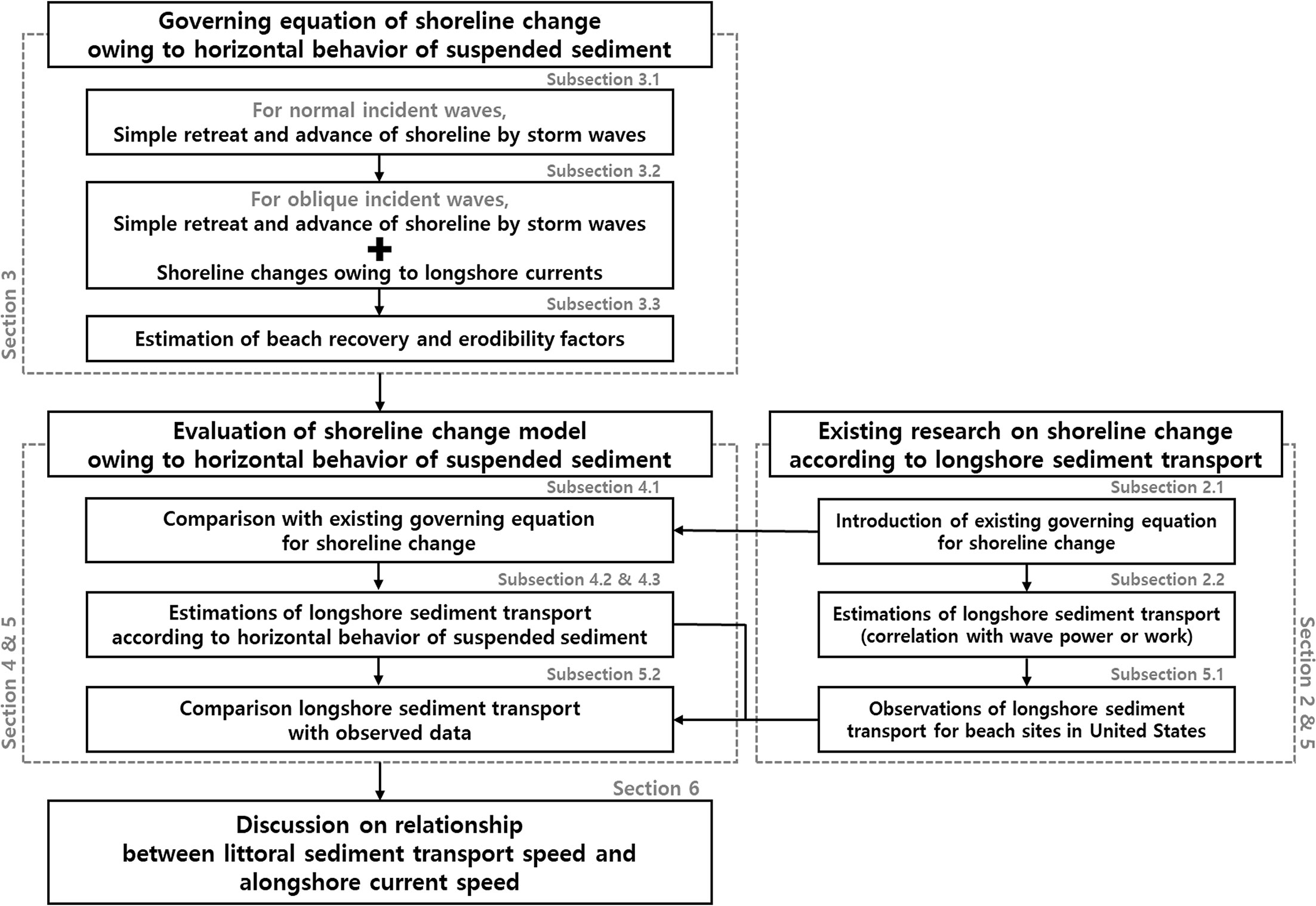
Figure 1 Workflow on the derivation of a governing equation for a short-term shoreline response model and comparative verification in terms of longshore sediment transport.

2 Existing governing equation for shoreline change

2.1 Existing governing equation for shoreline change

Pelnard-Considère (1956) derived the first analytic solution to describe shoreline change by assuming that the beach profile within the vertical height D_s always responds with the same shoreline retreat; therefore, the cross-shore fluxes were neglected. Thus, the temporal change in shoreline position y was obtained as described below by the difference in the LSTR Q_l entering and exiting the control volume:

$\begin{array}{ll}\frac{\partial y}{\partial t}=\frac{1}{D_s}\frac{\partial Q_l}{\partial x}& (1)\end{array}$

In the above equation, x is the alongshore coordinate and D_s is the height of the active profile at which the LSTR drifts along the shore. As shown in Figure 2, it is assumed that the increase or decrease of the LSTR uniformly occurs between these vertical heights, causing a change of the same Δy width. However, despite these assumptions, it is useful for simulating shoreline changes due to LSTR changes that occur when groynes or jetties are placed along the shore.

FIGURE 2

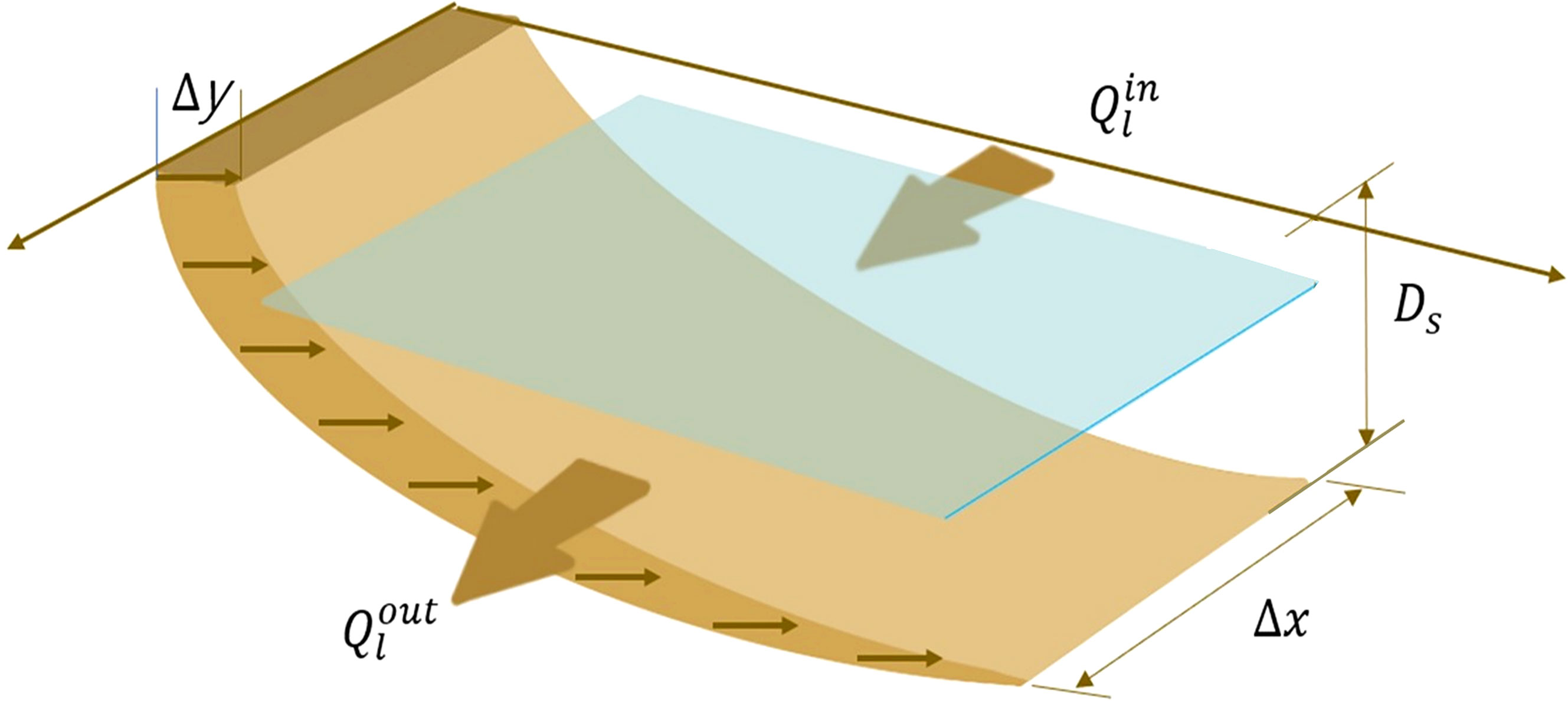
Figure 2 Definition sketch of an existing one-line shoreline change model.

2.2 Estimation of LSTR (LSTR–mass)

2.2.1 Estimation by wave power

Komar and Inman, (1970) considered that the transport rate of sediment drifting along the shore occurs because of wave action when the shoreline and incident wave direction form an oblique angle. Therefore, the LSTR Q_l [m³/s] integrated along the entire beach cross-section can be expressed as the immersed weight transport rate I_y, and I_y can be expressed as the product of the energy flux component P_l in the longshore direction at the breaking point, and the empirical constant K, which is the calibration coefficient:

$\begin{array}{ll}{Q}_l=\frac{I_y}{(s-1)(1-p)\rho g}=\frac{K{P}_l}{\left(s-1\right)(1-p)\rho g}& (2)\end{array}$

In the above equation, s is the specific gravity of the sediment, p is the porosity of the sediment, g is the acceleration due to gravity, and ρ is the density of the seawater. Therefore, LSTR can be extracted by substituting the longshore component of the energy flux into Eq. (2).

Among the various types of LSTR formulae, the CERC (1984) formula is the most widely used, as expressed in the form of the LSTR–mass:

$\begin{array}{ll}\dot{M_l}=\frac{{\rho }_s}{({\rho }_s-\rho )g}K{P}_l=K\frac{{\rho }_s}{({\rho }_s-\rho )g}{\left(E{C}_g\right)}_b\cos {\theta }_b\sin {\theta }_b& (3)\end{array}$

In the above equation, ρ_s is the density of sand, P_l is the wave energy flux, E is the total wave energy, C_g is the wave group velocity, and θ_b is the wave angle between the wave crest line and shoreline at breaking. The subscript b represents “breaking waves”. Here, if the wave energy or wave height is the value corresponding to the significant wave height, a K value of 0.39 is presented by CERC (1984). And Ṁ_l [kg/s] is the dry mass transport rate per unit time; thus, there is a relationship between Ṁ_l and Q_l:

$\begin{array}{ll}\dot{M_l}={\rho }_s\left(1-p\right)Q_l& (4)\end{array}$

To enhance the applicability of Eq. (2), Kamphuis (1991) identified a relationship for estimating the LSTR–mass based on an extensive series of laboratory tests and a broad set of field data, as given below:

$\begin{array}{ll}\dot{M_l}=2.33\frac{{\rho }_s}{{\rho }_s-\rho }{T}_p^{1.5}{m}_b^{0.75}{D}_{50}^{-0.25}{H}_b^2{\sin }^{0.6}(2{\theta }_b)& (5)\end{array}$

In the above equation, H_b is the breaking wave height, T_p is the peak wave period, m_b is the beach slope, and D₅₀ is the median grain size. Equation (5) is valid for both laboratory and field sand transport rates (Reeve et al., 2012). The Kamphuis (1991) formula was further modified by Mil-Homens et al. (2013) to give the modified Kamphuis (1991) formula, as follows:

$\begin{array}{ll}\dot{M_l}=0.15\frac{{\rho }_s}{{\rho }_s-\rho }{T}_p^{0.89}{m}_b^{0.86}{D}_{50}^{-0.69}{H}_b^{2.75}{\sin }^{0.5}(2{\theta }_b)& (6)\end{array}$

Both the original (Eq. (5); Kamphuis, 1991) and modified (Eq. (6); Mil-Homens et al., 2013) formulae are expressed in terms of the wave height, wave period, beach slope, and particle grain size.

Subsequently, van Rijn (2014) verified the applicability of the above formulae using 22 field data points, and further proposed a variation of the LSTR–mass formula called the CROSMOR model, which can be applied to both sand and gravel beaches, as follows:

$\begin{array}{ll}\dot{M_l}=0.00018{\rho }_s{g}^{0.5}{m}_b^{0.4}{D}_{50}^{-0.6}{H}_b^{3.1}\sin \left(2{\theta }_b\right)& (7)\end{array}$

In Section 5, the four LSTR–mass formulae in Eqs. (3) and (5) – (7) are compared with the LSTR–mass formula derived in this study.

2.2.2 Evaluation by wave work

Bayram et al. (2007) proposed a formula for the total LSTR that differs somewhat from conventional research results with respect to the principles of sediment transport physics, as it assumes that waves mobilize sediment, which is subsequently transported by current. That is, assuming that the work required for sediments to be suspended is called W, and only as much is used as the ϵ_B that is part of the wave energy flux at the breaking point F_b, the following equation is presented:

$\begin{array}{ll}W=(s-1)g{w}_s{\int }_0^{y_b}{\int }_{-h\left(y\right)}^{0}c\left(y,z\right)dzdy={ϵ}_B{F}_b& (8)\end{array}$

In the above equation, c is the suspended sediment concentration, w_s is the settling velocity of the suspended sediment, z is the vertical coordinate from the mean sea level to the seabed, and h is water depth. ϵ_B is the transport coefficient representing the efficiency with which the wave energy flux suspends the sediment (Bayram et al., 2007).

Assuming a constant (or representative) longshore current velocity and replacing the integral with the fraction of the incoming wave energy that is used to keep the sediment in suspension, the LSTR–mass can be obtained simply by taking the product of concentration and mean longshore current velocity:

$\begin{array}{ll}\dot{M_l}=\frac{{\rho }_s{ϵ}_B}{({\rho }_s-\rho )g{w}_s}{F}_b\overline{U_l}& (9)\end{array}$

In the above equation, $\overline{U_l}$ is the representative longshore current velocity, which is the average current across the beach profile based on the mean sea level along the surf zone. And the product of ϵ_B and $\overline{U_l}$ can be considered the littoral transport speed, representing the actual movement rate of suspended sediment.

Bayram et al. (2007) expressed the wave energy flux F_b under the action of oblique-incidence waves at the breaking point θ_b as follows:

$\begin{array}{ll}{F}_b=E_b{C}_{gb}\cos {\theta }_b& (10)\end{array}$

If the representative longshore current $\overline{U_l}$ in Eq. (9) is substituted by the equation proposed by Larson and Kraus (1991), the following result is obtained:

$\begin{array}{ll}\dot{M_l}=\frac{135}{256}\frac{\pi \gamma }{c_f}{ϵ}_B\frac{{\rho }_s}{({\rho }_s-\rho )g}{E}_b{C}_{gb}\cos {\theta }_b\sin {\theta }_b=258.45{ϵ}_B\frac{{\rho }_s}{({\rho }_s-\rho )g}{E}_b{C}_{gb}\cos {\theta }_b\sin {\theta }_b& (11)\end{array}$

In the above equation, c_f is the friction coefficient, and γ is the breaker index. Bayram et al. (2007) obtained the representative value of ϵ_B=3.9×10^–3K, when compared to the CERC (1984) formula.

3 Shoreline change owing to the horizontal behavior of suspended sediment

3.1 Shoreline change by normal incident wave

When the incident wave energy is dissipated along a beach slope, sediment particles are picked up and suspended in flowing water. When the incident energy subsides, the suspended sediment then settles shoreward. Figure 3 illustrates this process, where sediment particles are suspended during episodes of turbulent energy, followed by precipitation under gravity once the energy dissipates. These approaches to seabed changes by vertical erosion and settlement have already appeared in the literature (Partheniades, 1965; Hanson, 1990; Hanson and Cook, 1997). In this paper, because shoreline retreat and recovery are repeated horizontally, as is done vertically in the seabed, the behavior of suspended sediments on the beach is approached as horizontal disengagement and recovery rather than vertical erosion and settlement.

FIGURE 3

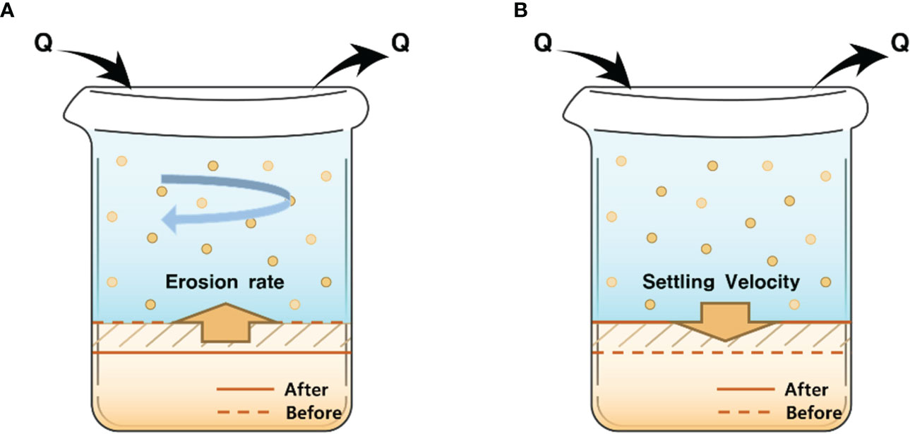
Figure 3 Vertical behavior of suspended sediments in a gravitational field: (A) seabed deepening due to sediment suspension and (B) seabed recovering owing to sediment settling.

Thus, this study derives a mathematical equation for the horizontal behavior of suspended sediments, in a manner similar to the methods already applied to the vertical behavior (Partheniades, 1965; Hanson, 1990; Hanson and Cook, 1997, 2004). First, assuming that suspended sediment is transported horizontally, the temporal change in the shoreline position where water and land meet at a constant sea level can be expressed as follows (Kim et al., 2021; Lim et al., 2022b):

$\begin{array}{ll}\frac{d{y}_r}{dt}=\frac{1}{D_s(1-p)}(q_D^c-q_E^c)& (12)\end{array}$

In the above equation, t is the sand migration time, y_r is the cross-shore retreated location, which is positive in the onshore direction from the initial shoreline, and superscript “c” represents cross-shore. The parameter $q_D^c$ [m²/s] is the deposition rate due to the recovery process of suspended sediment, and $q_E^c$ [m²/s] is the entrainment rate of suspended sediments due to wave energy dissipation. This model has the advantage of being able to simulate episodic shoreline retreat and recovery under storm wave conditions. Although sea level changes (e.g., wave setup, tides, and sea level rise) are not considered separately in this paper, shoreline changes considering sea level changes can be easily simulated by adding corresponding terms (Lim et al., 2022b). Sea level changes should be taken into account if the shoreline sensitively responds to them due to large tidal differences or mild beach slopes.

The entrainment rate $q_E^c$ is expressed as a function of the wave energy exerted at the starting point of wave breaking (Kim et al., 2021; Lim et al., 2022b), as follows:

$\begin{array}{ll}\frac{q_E^c}{D_s(1-p)}=\frac{m{E}_b^{\text{'}}}{\left(s-1\right)\left(1-p\right)}& (13)\end{array}$

In the above equation, $E_b^{\text{'}}$ [m²] is the value of the wave energy E_b divided by $\rho g$ ($E_b^{\text{'}}=E_b/\rho g$), and m [1/(m·s)] is the beach erodibility factor. The parameter $q_D^c$ is expressed as a function of the cross-shore integrated concentration C_s (Kim et al., 2021; Lim et al., 2022b), as follows:

$\begin{array}{ll}\frac{q_D^c}{D_s(1-p)}=\frac{k_r{C}_s}{\left(s-1\right)\left(1-p\right)}& (14)\end{array}$

In the above equation, k_r [1/s] is the beach recovery factor with units of the reciprocal of time, which represents the rate at which the suspended sediment returns shoreward; its value depends on the sediment characteristics; C_s [m] is the cross-shore integrated concentration divided by ρ, which is the amount of suspended sediment divided by the unit area (product of the vertical range and unit longshore width).

When Eq. (12) reaches equilibrium, C_s reaches the condition:

$\begin{array}{ll}{C}_s=\frac{m{E}_b^{\text{'}}}{k_r}& (15)\end{array}$

Moreover, Δy_r, which indicates the retreat displacement of the shoreline position in the cross-shore direction, can be expressed by C_s:

$\begin{array}{ll}\Delta y_r=\frac{C_s}{\left(s-1\right)\left(1-p\right)}& (16)\end{array}$

3.2 Shoreline change by oblique incident wave

Section 3.1 summarizes the process of interpreting the simple retreat and advance of the shoreline as the horizontal behavior of suspended sediments caused by storm waves, ignoring changes in the shoreline owing to the longshore sediment transport. And in this section, by extending the previous section to the case of oblique incident waves, the transport and diffusion of suspended sediments are analyzed to show not only shoreline retreat and recovery by storm waves but also additional shoreline changes owing to longshore currents. In this process, the governing equation for the transport and diffusion of suspended sediments is introduced. For normal incident waves, C_s is meaningless because Eq. (16) is satisfied. However, for oblique incident waves, C_s can be solved with the help of the transport and diffusion equation of suspended sediments because C_s undergoes a change along the shoreline.

When a wave enters the shore at an oblique angle, $q_D^c$, the rate at which suspended sediment returns to the original shoreline position is valid, as in the normal wave environment, as shown in Eq. (14). However, the erosion rate $q_E^c$ at which sand moves away from the shore, given in Eq. (13), is affected by the oblique wave angle. In other words, for a wave where the crest enters obliquely at an angle of cosθ_b, the shoreline length affected by wave energy is longer by 1/cosθ_b, compared to normal incidence. Therefore, the following results were obtained for the deposition rate $q_E^c$:

$\begin{array}{ll}\frac{q_E^c}{D_s(1-p)}=\frac{m{E}_b^{\text{'}}}{(s-1)(1-p)}\text{c}\text{o}\text{s}{\theta }_b& (17)\end{array}$

When applying these results to oblique angle wave environments, the receding shoreline position for each control volume can be expressed as follows:

$\begin{array}{ll}\frac{d{y}_r}{dt}=\frac{1}{(s-1)(1-p)}(k_r{C}_s-m{E}_b^{\text{'}}\text{c}\text{o}\text{s}{\theta }_b)& (18)\end{array}$

The C_s in Eq. (14) is affected by the difference in sediment transport rates entering and exiting the control volume. Therefore, the following equation is required to analyze the transport and diffusion of suspended sediments along the shore:

$\begin{array}{ll}\frac{\partial C_s}{\partial t}+\frac{\partial {\overline{U}}_{ls}{C}_s}{\partial x}=D\frac{{\partial }^2{C}_s}{\partial x^2}+m{E}_b^{\text{'}}\text{c}\text{o}\text{s}{\theta }_b-k_r{C}_s& (19)\end{array}$

In the above equation, ${\overline{U}}_{ls}$ [m/s] is the littoral transport speed, and D [m/s] is the diffusion coefficient of the suspended sediment in the longshore direction.

Therefore, when the wave enters at an oblique angle, the following relationship is established for C_s under the condition that Eq. (18) reaches the equilibrium:

$\begin{array}{ll}{C}_s^E=\frac{m{E}_b^{\text{'}}\text{c}\text{o}\text{s}{\theta }_b}{k_r}& (20)\end{array}$

In the above equation, the superscript ‘E’ represents equilibrium.

Equations (18) and (19) are the material conservation laws of sediment applied to the land and water bodies of a beach, respectively, where Eq. (18) describes the temporal changes in the shoreline boundary, whereas Eq. (19) describes the temporal change in the sediment load suspended in water. Together, they represent the sediment load entering the control volume of water from the land due to wave breaking and the sediment load returning from the control volume to the shore by the sediment recovery process. In longshore sediment transport, the amount of suspended sediment D_sC_s is determined by littoral transport speed ${\overline{U}}_{ls}$, as shown in Figure 4.

FIGURE 4

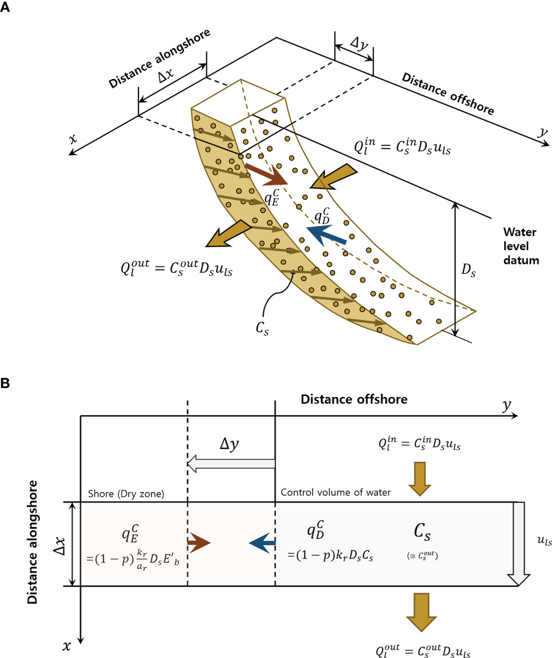
Figure 4 Sediment transport and shoreline change according to the horizontal behavior of suspended sediment under oblique wave incidence: (A) three-dimensional view (B) plan view.

Figure 4 shows a conceptual diagram in which the amount of suspended sediment D_sC_s is transported at littoral transport speed ${\overline{U}}_{ls}$ during longshore sediment transport. It also shows that the shoreline responds to differences in both cross-shore and longshore sediment transport rates. Further details are provided in Section 4.

3.3 Beach erodibility and recovery factors

Miller and Dean (2004) attempted to determine whether the beach recovery factor k_r is a constant function of the breaking wave height H_b or a function of the disequilibrium factor Ω from the temporal evolutionary pattern of shoreline location. They found that none of the specified options considered for k_r were dominant. However, Lim et al. (2022c) showed that k_r can be expressed as a beach size factor A, as follows:

$\begin{array}{ll}{k}_r\cong \frac{2.3 A^{3/2}}{\left(1+14A^{3/2}\right)}& (21)\end{array}$

The above equation is based on the statistical analysis of a 10-year shoreline survey dataset acquired along the east coast of Korea, with differing D₅₀ values and numerical results obtained through storm wave scenario functions. Lim et al. (2022c) also reported that the beach erodibility factor m can be expressed in terms of beach scale factor A, as follows:

$\begin{array}{ll}m\cong \left(s-1\right)\left(1-p\right)\frac{20}{\left(1+14A^{3/2}\right)}& (22)\end{array}$

Therefore, for a given beach scale factor A, the beach erodibility factor m and beach recovery factor k_r can be readily estimated and applied to the shoreline changes. The m and k_r are two key physical coefficients related to suspended sediment transport, and the fact that they can be obtained as beach scale factor A in advance increases the convenience of using the proposed governing equation. In addition, the reliability of the results can be obtained in that the beach recovery and erodibility factors are not adjusted from the simulated results. The equations for the two physical coefficients were mainly verified on the east coast of Korea. However, because both equations were applied to 11 straight beaches with different particle sizes, it is assumed that they can be applied to other areas directly exposed to open sea waves.

4 Evaluation of the proposed governing equation

4.1 Comparison with the existing governing equation for shoreline change

The governing equation proposed in this study was derived to simulate shoreline changes caused by transverse and littoral drifts. Therefore, compared to the existing governing equation given in Eq. (1), the shoreline changes due to the transverse transport of suspended sediment were included. If the shoreline change caused by transverse sediment transport is ignored, Eq. (18) is irrelevant; and if the transverse sedimentation and diffusion terms are removed from Eq. (19), it can be expressed as follows:

$\begin{array}{ll}\frac{\partial C_s}{\partial t}+\frac{\partial {\overline{U}}_{ls}{C}_s}{\partial x}=0& (23)\end{array}$

In the above equation, C_s can be expressed as C_s=(s–1)(1–p)Δy_r, as given in Eq. (16). The ${\overline{U}}_{ls}{C}_s$ in Eq. (23) corresponds to littoral drift (s–1)(1–p)Q_l/D_s. Therefore, the C_s and ${\overline{U}}_{ls}{C}_s$ included in Eq. (23) can be expressed as (s–1)(1–p)Δy_a and (s–1)(1–p)Q_l/D_s, respectively. Equation (23) becomes the same as Pelnard-Considère’s (1956) equation given in Eq. (1). Here, $\Delta y_a$ is in the opposite direction to Δy_r and indicates the forward advancing motion of the shoreline.

4.2 LSTR–mass in equilibrium state

LSTR–mass $\dot{M_l}$ can be obtained as the product of the sediment concentration and sediment discharge rate in the longshore direction. Applying the horizontally integrated volumetric concentration in equilibrium $C_s^E$ and using the representative littoral transport speed ${\overline{U}}_{ls}$, the LSTR of the dry sediment mass $\dot{M_l}$ can be expressed as follows:

$\begin{array}{ll}\dot{M_l}={\rho }_s\left(1-p\right)\frac{C_s^E}{(s-1)(1-p)}{D}_s{\overline{U}}_{ls}=\frac{{\rho }_s}{({\rho }_s-\rho )g}\frac{m{E}_b\text{c}\text{o}\text{s}{\theta }_b}{k_r}{D}_s{\overline{U}}_{ls}& (24)\end{array}$

In the above equation, the ${\overline{U}}_{ls}$ is considered the product of ${ϵ}_L$ and $\overline{U_l}$, as described in Section 2. Suspended sediment moves along the wave-induced longshore current caused by oblique wave incidence, but considering the weight of the sediment and the movement, mainly along the shore bottom, the actual sediment movement speed ${\overline{U}}_{ls}$ is lower than the seawater movement speed. Therefore, the ϵ_L is taken as the delay factor of longshore sediment transport (DFLST), which indicates the difference in speed between ${\overline{U}}_{ls}$ and U_l. Although LSTR–mass and DFLST do not have the same meaning, the fact is that the LSTR–mass being expressed by introducing a small calibration coefficient in CERC (1984) or van Rijn (2014) is a naturally inherent result of the physical meaning of this DFLST.

If ${\overline{U}}_{ls}$ is expressed as ${ϵ}_L{\overline{U}}_l$, then Eq. (24) is expressed as a term of ${ϵ}_L{\overline{U}}_l$ as follows, for which considerable research has already been conducted:

$\begin{array}{ll}\dot{M_l}=\frac{{ϵ}_L{\rho }_s}{({\rho }_s-\rho )g}\frac{m{E}_b\text{c}\text{o}\text{s}{\theta }_b}{k_r}{D}_s{\overline{U}}_l& (25)\end{array}$

Various empirical formulae have been proposed for wave-induced currents; however, in this study, applying the following formula derived by Bayram et al. (2007) yielded the same result as the CERC formula in terms of θ_b:

$\begin{array}{ll}{\overline{U}}_l=\frac{5}{32}\frac{\pi \gamma \sqrt{g}}{c_f}{A}^{3/2}\sin {\theta }_b& (26)\end{array}$

Therefore, by substituting Eq. (26) into Eq. (25), LSTR–mass Ṁ_l under the equilibrium condition is expressed as follows:

$\begin{array}{ll}\dot{M_l}=\frac{5}{32}\frac{\pi \gamma \sqrt{g}}{c_f}\frac{{ϵ}_L{\rho }_s}{({\rho }_s-\rho )g}\frac{m}{k_r}{A}^{3/2}{D}_s{E}_b\text{c}\text{o}\text{s}{\theta }_b\sin {\theta }_b& (27)\end{array}$

In the above equation, the beach erosion factor m and beach recovery factor k_r are the main physical parameters and are given in Eqs. (21) and (22), respectively; by applying these equations to Eq. (27), we obtain the following simplified form:

$\begin{array}{ll}\dot{M_l}=1.3587{\rho }_s\left(1-p\right)\frac{\pi \gamma }{c_f\rho \sqrt{g}}{ϵ}_L{D}_s{E}_b\text{c}\text{o}\text{s}{\theta }_b\sin {\theta }_b& (28)\end{array}$

Then when compared to the CERC (1984) formula, the DFLST ϵ_L is expressed as a function of K, as follows:

$\begin{array}{ll}{ϵ}_L=\frac{c_f}{1.3587\pi \gamma \sqrt{g}\left(s-1\right)\left(1-p\right)}\frac{\sqrt{g{h}_b}}{D_s} K=4\text{.}8432\times 10^{-4}\frac{C{ }_{\mathrm{gb}}}{D_s} K& (29)\end{array}$

To obtain the second term, a friction factor c_f of 0.005 and breaker index γ of 0.78 were applied.

4.3 Estimation of littoral transport speed

If littoral transport speed ${\overline{U}}_{ls}$is expressed as the product of ϵ_L and ${\overline{U}}_l$, the following equation is obtained:

$\begin{array}{ll}{\overline{U}}_{ls}=0.1162\frac{C_{gb}}{D_s} K{A}^{3/2}\sin {\theta }_b& (30)\end{array}$

Here, K has been suggested by many scholars to be related to D₅₀, and A has been presented in terms of D₅₀ by Dean (1987). Therefore, we will attempt to express KA^3/2 as a function of A by examining how the three representative expressions for K (Swart, 1976; del Valle et al., 1993; Coastal Engineering Manual, 2002) can be implicitly expressed as a function of A.

First, the formula proposed by Swart (1976) as a function of the median grain size D₅₀ for the sediment transport coefficient K is expressed as follows:

$\begin{array}{ll}K=0.575 \text{log}{ }_{10}\left(0.00146/D_{50}\right)& (31)\end{array}$

In the above equation, D₅₀ is given in meter units, and the above formula is valid for 0.1 mm< D₅₀<1.0 mm.

del Valle et al. (1993) proposed the following equation showing the exponential decrease in K when the D₅₀ increases, based on the results of Komar (1988) and the data obtained from the Adra River Delta in Spain:

$\begin{array}{ll}K=0.8 \text{e}\text{x}\text{p}\left(-2.5·D_{50}\right)& (32)\end{array}$

In the above equation, D₅₀ is given in mm units.

Coastal Engineering Manual (2002) reported that the D₅₀ and K have the following relationship, based on the data of Komar (1988), Nicholls and Webber (1987), and Chadwick et al. (1989):

$\begin{array}{ll}K=\frac{0.1}{D_{50}}& (33)\end{array}$

In the above equation, D₅₀ is given in mm units.

Figure 5 shows the relationship between the three formulae for K and the beach scale factor A. Swart (1976) and del Valle et al. (1993) show a linear relationship with A in the range 0.1 mm< D₅₀<1.0 m. The Coastal Engineering Manual (2002) shows a similar relationship with A^–2 in the range (0.17 mm< D₅₀<1.0 mm). In this study, we selected $K\cong 0.005A^{-2}$, which shows a similar tendency to the formula provided by the Coastal Engineering Manual (2002), which is a recent research outcome, and produces more neatly arranged mathematical results. Therefore, by removing the CERC (1984) empirical constant K shown in Eq. (30), the littoral transport speed is approximately expressed as the beach scale factor A, in meter units, as follows:

FIGURE 5

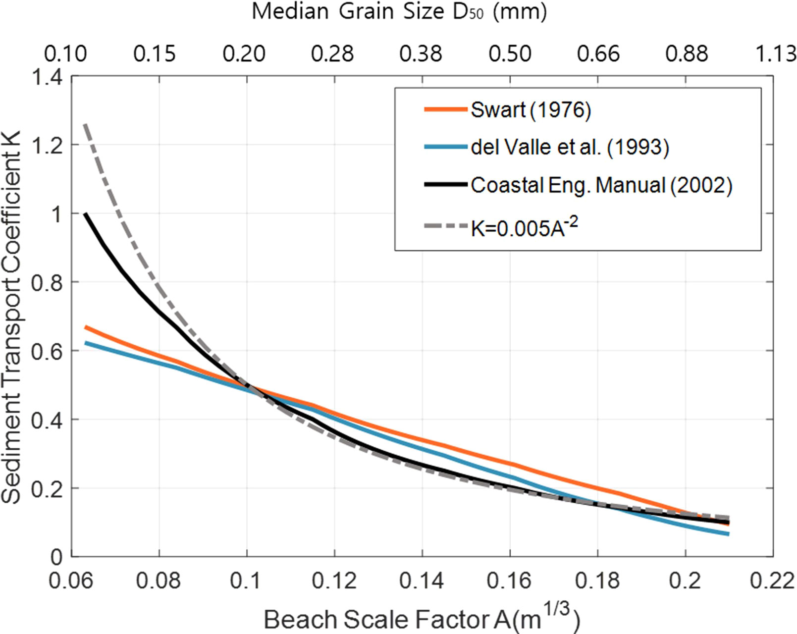
Figure 5 Variation of K value with respect to the beach scale factor A.

$\begin{array}{ll}{\overline{U}}_{ls}=5.81\times {10}^{-4}{A}^{-1/2}\frac{C_{gb}}{D_s} \text{s}\text{i}\text{n}{\theta }_b& (34)\end{array}$

This implies that if the other conditions are the same, as A (D₅₀) increases, the movement speed of sand decreases. Section 5 details which of these equations gives the most similar results to the LSTR–mass observations.

5 Comparison with observed LSTR–mass

5.1 LSTR–mass observations

The LSTR–mass field datasets from 25 beach sites in the United States (USA), as shown in Table 1, were selected for comparison with the LSTR–mass, which was calculated using the new suspended sediment model and four other conventional equations (discussed in Section 2.1). The field datasets were broadly divided into three groups based on the magnitude of the observed LSTR–mass (Watts, 1953; Moore and Cole, 1960; Lee, 1975; Lee, 1975; Kana, 1977; Kana and Ward, 1980; Gable, 1981; Kraus and Dean, 1987; Wang et al., 1998; Miller, 1999; Wang and Kraus, 1999), including Indian Rocks Beach, an area with a low LSTR–mass, Duck Beach, with a high LSTR–mass, and the remaining sites with an intermediate LSTR–mass.

TABLE 1

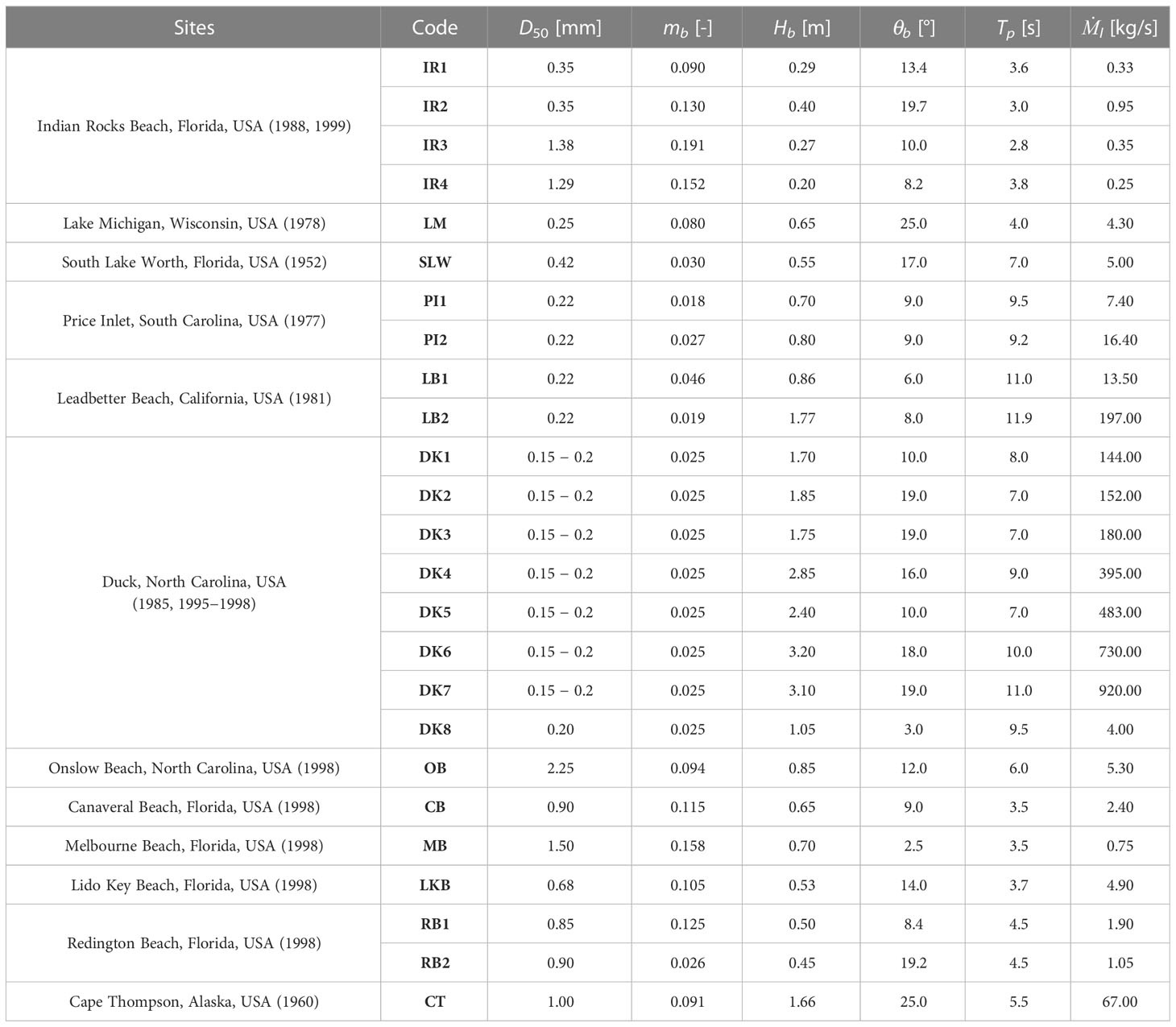
Table 1 Field data for LSTR–mass for 21 beach sites in the United States (van Rijn, 2002; van Rijn, 2014).

The Indian Rocks Beach in Florida has a low LSTR–mass due to its small wave height and tidal range, with medium sand (0.35 mm). Wang and Kraus (1999) obtained the LSTR–mass by observing topographic changes over a short period (< 1 d). Duck, North Carolina has a high LSTR–mass due to high waves, a relatively long period, a small tidal range, and fine sand of (0.15 – 0.2) mm. Kraus and Dean (1987) determined LSTR–mass using streamer traps during swell waves in 1985 and 1995−1998. Miller (1999) monitored the LSTR–mass using electronic concentration sampling during storm conditions.

In the intermediate LSTR–mass group, the South Lake Worth beach in Florida has a small tidal range with coarse sand of (0.4 − 0.6) mm. Watts (1953) obtained the LSTR–mass from sand bypassing a sand pumping plant. Additionally, the beach at Lake Michigan, Wisconsin has fine sand of (0.2 − 0.3) mm and small waves. Lee (1975) calculated the LSTR–mass using trap samplers. Leadbetter Beach in California and Price Inlet in South Carolina also have fine sand of (0.2 − 0.25) mm. The LSTR–mass in Leadbetter Beach was reported by Gable (1981) due to topographic changes over one year, whereas the LSTR–mass at Price Inlet was collected using trap samplers (Kana, 1977; Kana and Ward, 1980).

Schoonees and Theron (1993; 1996) recalibrated the LSTR–mass equation of Kamphuis (1991) using 123 data points from their field dataset and obtained similar results. Up to this stage, most of the field data were for wave heights< 2 m in the open sea, and a median sand grain size of approximately (0.2 − 0.6) mm. Field data for the LSTR–mass for higher waves were provided by Miller (1999), who reported observations conducted by the US Army Corps of Engineers (USACE) at Duck, North Carolina from 1995 to 1998. van Rijn (2014) summarized 25 field datasets from Schoonees and Theron (1993; 1996) and Miller (1999) (Table 1) to verify the proposed LSTR–mass equations, in which D₅₀ranged from (0.15 − 0.42) mm.

Additionally, for coarse sand, Wang et al. (1998) used streamer traps to observe LSTR–mass at various beaches around the southeast coast of the US and the Gulf Coast of Florida. Wang et al. (1998) noted that the observed LSTR–mass may have been underestimated because it was observed with a duration of approximately 5 minutes using streamer traps. Moore and Cole (1960) also observed LSTR–mass for coarse sand in Cape Thompson, northwestern Alaska, USA. Moore and Cole (1960) observed wave conditions higher than those investigated by Wang et al. (1998) and observed LSTR–mass by observing temporal changes on the spit along the outlet of a lagoon along the spit at Cape Thompson for a duration of approximately 3 hours.

5.2 Comparison with observed data

To verify the LSTR–mass obtained by applying Eq. (34) for the littoral transport speed, we compared it with the values of the four conventional LSTR–mass equations. This result corresponds to the CERC (1984) equation because the DFLST was obtained by comparison with the CERC (1984) formula. However, the application of a constant K value (0.39) was regarded as the result of the CERC (1984) formula, and the application of K=0.005A^–2 was regarded as the LSTR–mass by the governing equation of this study. Dean (1977) provided beach scale factor A on American sand beaches in the range of (0.1 − 1.0) mm median grain size. Therefore, in this study, LSTR–mass observation data on beaches with a median grain size sand of (0.1 − 1.0) mm were applied.

Table 2 lists the correlation coefficients and root mean squared log error (RMSLE) of the comparison results. The LSTR–mass obtained in this study showed the lowest RMSLE. Figure 6 compares the LSTR–mass data and computed LSTR–mass results.

TABLE 2

Table 2 Calculation of LSTR–mass from new suspended sediment model proposed in the present study and four conventional equations.

FIGURE 6

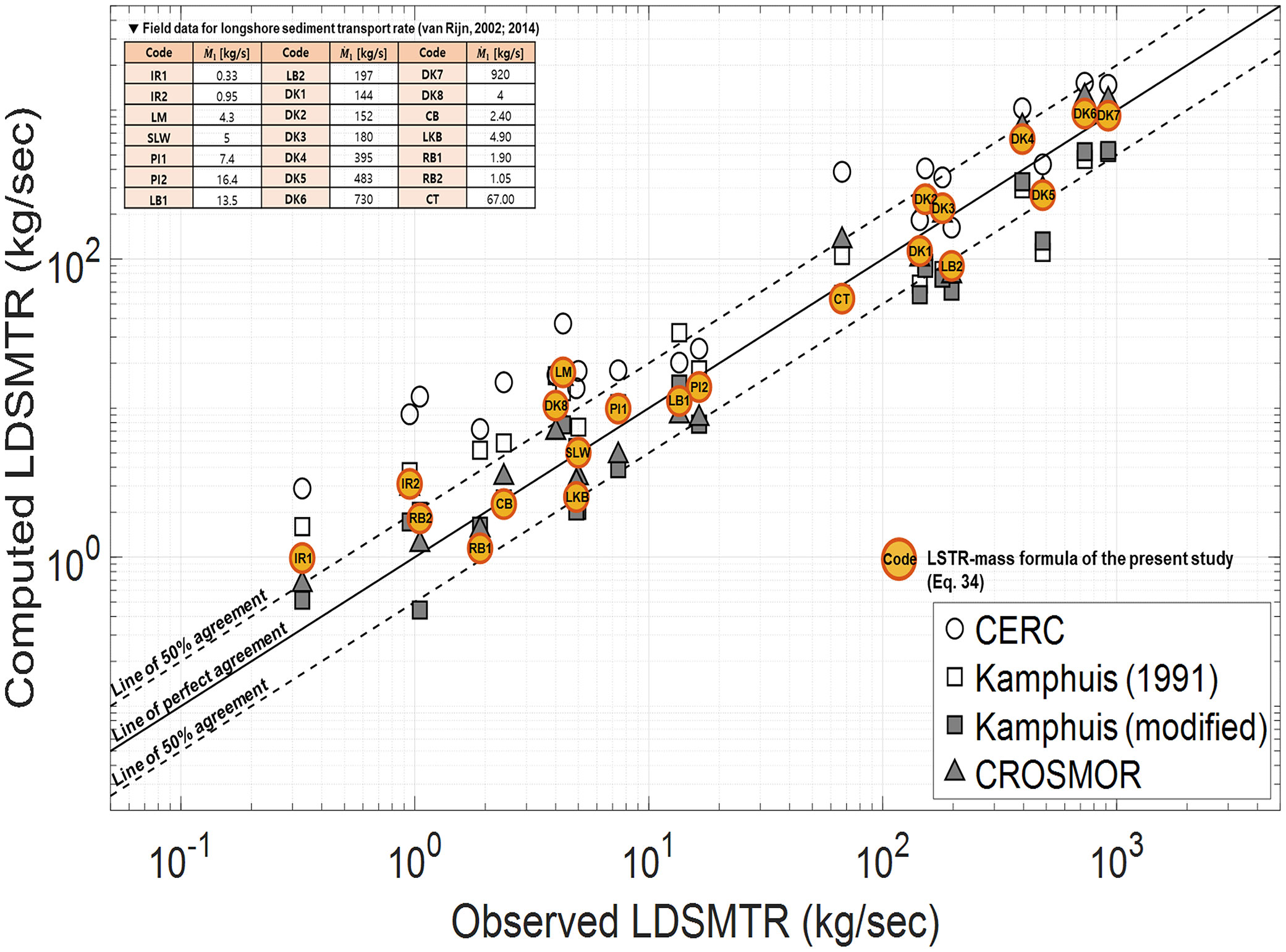
Figure 6 Comparison between observed LSTR-mass and calculated LSTR-mass (including Eq. (34) by the present study).

As a measure of scatter, the RMSLE was calculated as follows:

$\begin{array}{ll}RMSLE=\sqrt{\frac{{\sum }_{i=1}^N{(\text{l}\text{o}\text{g}(\dot{M_{lo}}+1)-\text{l}\text{o}\text{g}(\dot{M_{lc}}+1))}^2}{N}}& (35)\end{array}$

In the above equation, Ṁ_lo is the observed LSTR–mass, Ṁ_lc is the computed LSTR–mass, and N is the number of data points.

6 Discussion

6.1 Time evolution of LSTR

When waves enter the shore uniformly, the concentration of suspended sediment and the speed of littoral sediment ultimately reach equilibrium. However, when a storm wave with large wave height enters, it peaks after a relatively high wave occurs and then begins to subside again, so the concentration of suspended sediments or the LSTR falls short of equilibrium. Figure 7 shows the suspended sediment concentration, according to the elapsed time when a wave with constant wave height enters the straight shore at an oblique angle, as a case where the governing equations for shoreline change (see Eqs. (18) and (19)) that are proposed in this study are applied. Unlike the traditional shoreline change model, the phenomenon of lag of suspended sediment concentration occurs with the occurrence of waves, and if it is observed at the beginning of the wave inflow, or if the elapsed time is insufficient to reach equilibrium, the suspended sediment concentration will not reach equilibrium and decrease. Therefore, depending on the wave duration, the LSTR–mass value obtained in the actual field was lower than the calculated value.

FIGURE 7

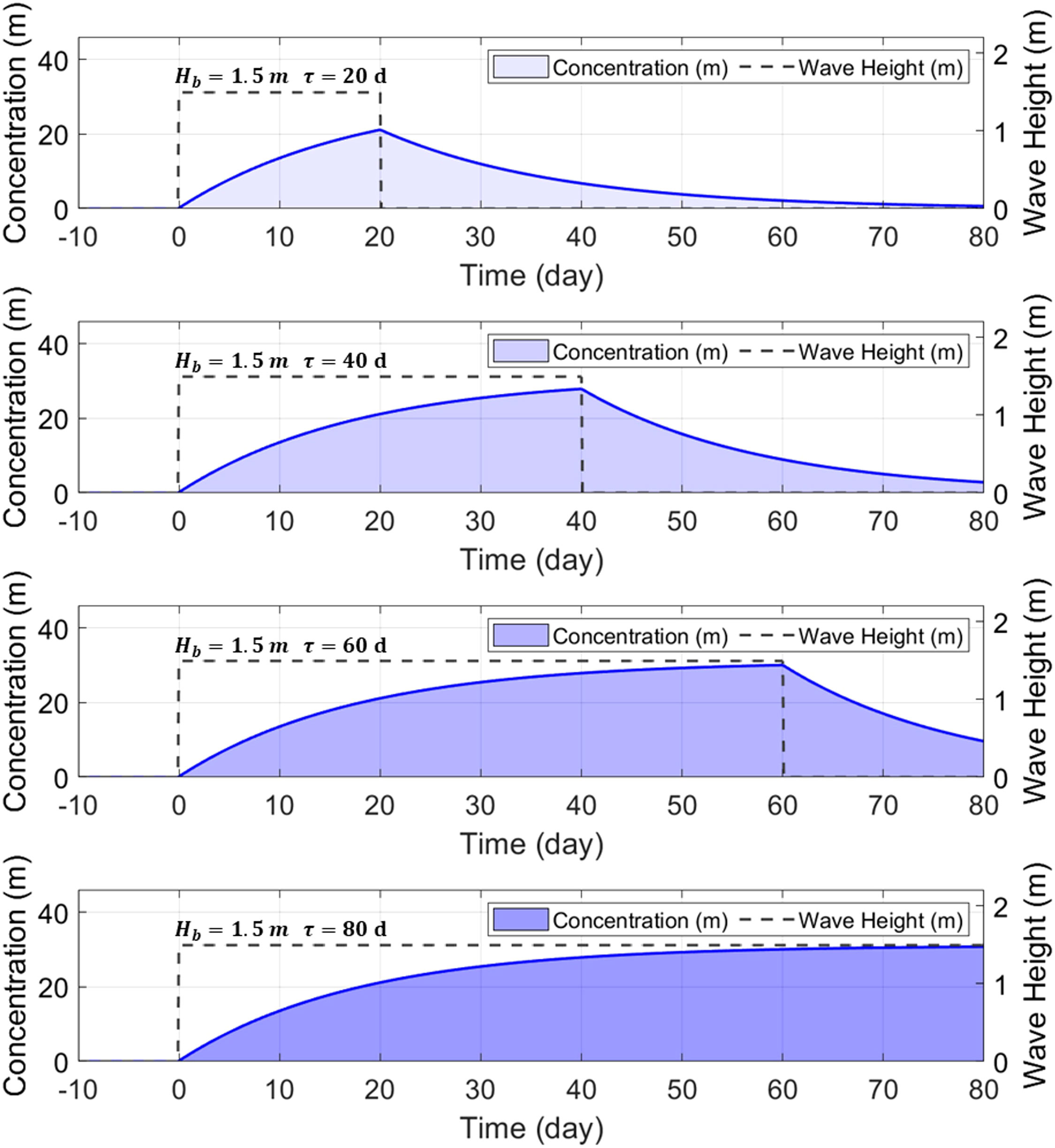
Figure 7 Temporal variation of suspended sediment concentration according to the incident duration of the uniform wave height.

Among the equations (Eqs. (18) and (19)) governing shoreline change, only Eq. (18) is effective because C_s does not change along the shoreline; and when applied to a straight beach, y_r in Eq. (18) can be expressed as C_s, as given in Eq. (16). Therefore, if the incoming wave conditions are constant, Eq. (18) is given by the following equation:

$\begin{array}{ll}\frac{d{C}_s}{dt}=k_r{C}_s-m{E}_b^{\text{'}}\text{cos}{\theta }_b& (36)\end{array}$

If the second term on the right-hand side is constant, then the solution of Eq. (36) becomes the following:

$\begin{array}{ll}{C}_s=\frac{m{E}_b^{\text{'}}\text{cos}{\theta }_b}{k_r}\left(1-\exp \left(-k_r\tau \right)\right)=\mu C_s^E& (37)\end{array}$

In the above equation, μ is the ratio of the concentration value according to the elapsed time τ to the concentration value when equilibrium is reached; since the peak rate μ_p occurs at τ, which is the wave duration, as shown in Figure 7, it is expressed as μ_p=1–exp(–k_r τ). In Eq. (37), C_s corresponds to the true value observed in the actual field, and $C_s^E$ is the value obtained assuming that equilibrium has been reached.

6.2 Correlation between the alongshore energy flux and wave duration

Table 3 shows the alongshore energy flux per unit length of beach, P_l and beach recovery factor, k_r, and the estimated rate μ from the observations for each site mentioned in the previous section. In Table 3, if the μ is 1 or more, the actual observed value is greater than the calculated LSTR value. However, if the suspended sediment concentration that has reached equilibrium is applied, as shown in Eq. (20), the μ must be less than 1 according to Eq. (37). Therefore, when estimating ϵ_L in Section 4.2, this means that ϵ_L must be determined so that the μ does not produce a result greater than 1. Nevertheless, comparing it with the CERC equation when estimating ϵ_L was intended to make the average value of μ nearly equal to 1.

TABLE 3

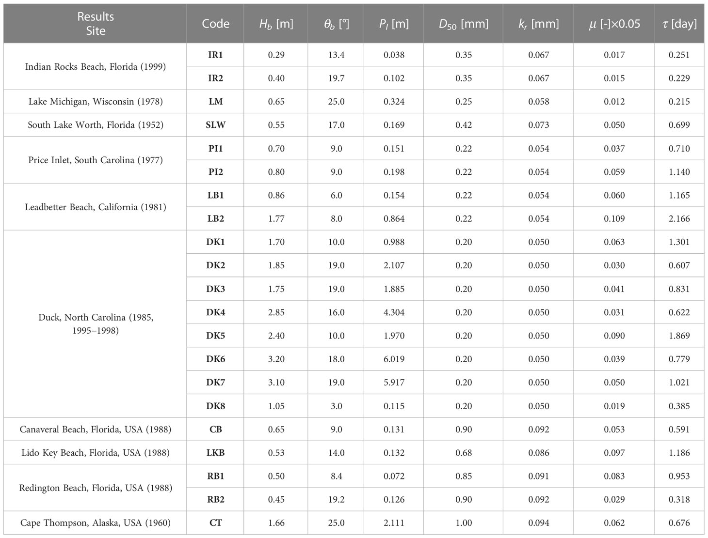
Table 3 The estimated ratio μ from observations and the adjusted wave duration τ.

Thus, the ϵ_L given in Section 4.2 is underestimated. To estimate how much it is underestimated, the duration data according to wave height and direction in the breaker line are applied, which were presented by Van Wellen et al. (2000). Figure 8 shows the duration for the alongshore energy flux per unit length of beach P_l. It can be seen that $\tau$ corresponding to wave duration is constrained by the following formula:

FIGURE 8

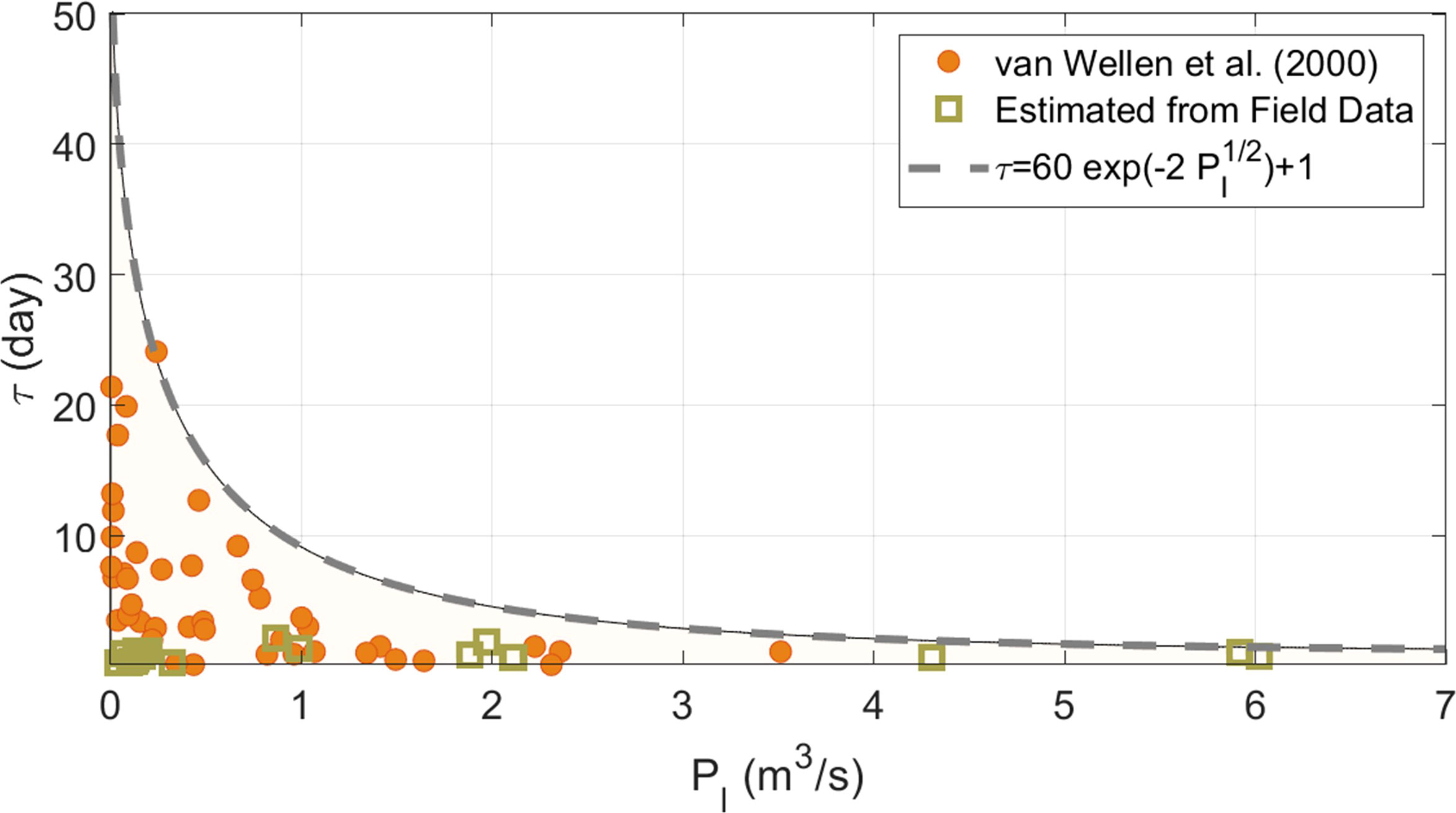
Figure 8 Wave duration τ with respect to the alongshore energy flux P_l.

$\begin{array}{ll}\tau =60\exp (-2P_l^{\frac{1}{2}})+1& (38)\end{array}$

The curve implies that the larger the P_l, the shorter the duration for which the wave lasts in the shore. Adjusting the μ by multiplying it by 1/20 so that the elapsed time t lies within this inclusive line shows a reasonable trend compared to the results obtained from the data from Van Wellen et al. (2000), as shown in Figure 8. In Table 3, the elapsed time t obtained by multiplying μ by 1/20 is also presented.

As the longshore component of energy flux increases, the duration tends to decrease. That is, it can be seen that the storm wave with high waves does not last long enough for the concentration of suspended sediment to reach equilibrium and shows an absurdly small duration. This result suggests that the existing LSTR estimation method (Komar and Inman, 1970), which ignores the evolutionary reaction between wave height (or energy flux) and suspended sediment concentration and immediately determines the LSTR according to wave height, has a large contradiction. The shoreline change model (Pelnard-Considère, 1956) is fundamentally difficult to escape from this contradiction. Therefore, this logically implies that the littoral transport speed mentioned in Section 4.3, ${\overline{U}}_{ls}$ must be approximately 20 times greater than the result obtained by comparing it to the CERC empirical equation, Eq. (34). Therefore, ϵ_L and ${\overline{U}}_{ls}$ should be modified as follows:

$\begin{array}{ll}{ϵ}_L=0.0097\frac{C_{gb}}{D_s} K\cong \frac{4.8432\times {10}^{-5}}{A^2}\frac{C_{gb}}{D_s}& (39)\end{array}$

$\begin{array}{ll}{\overline{U}}_{ls}=\frac{0.0116}{A^{1/2}}\frac{C_{gb}}{D_s} \text{sin}{\theta }_b& (40)\end{array}$

From Eq. (39), we get the following final relationship between ${\overline{U}}_{ls}$ and ${\overline{U}}_l$:

$\begin{array}{ll}{\overline{U}}_{ls}=0.0097\frac{C_{gb}}{D_s} K{\overline{U}}_l \cong \frac{4.8432\times {10}^{-5}}{A^2}\frac{C_{gb}}{D_s}{\overline{U}}_l& (41)\end{array}$

If the group velocity at breaking point $C_{gb}$ and the vertical height of active profile D_s are in the same order, it is estimated that for $K=0.39\left(A\cong 0.1132\right)$, the littoral sediment transport speed ${\overline{U}}_{ls}$ is approximately 0.0038 (=1/260) times slower than the alongshore current speed ${\overline{U}}_l$.

6.3 Relationship curves between the observed LSTR–mass and equilibrium LSTR–mass

If the relationship between the duration and the alongshore energy flux described in Section 6.2 is applied to the μ_p formula shown in Section 6.1, it can be seen how small the real LSTR values calculated according to k_r are compared to the equilibrium LSTR value. Figure 9 shows the relationship curves between the observed LSTR–mass and computed LSTR–mass in equilibrium state for the recovery factors k_r= (0.05, 0.10, 0.20, and 0.40) day⁻¹. The figure also indicates how small the LSTR observed in the field is compared to the equilibrium LSTR calculated according to the observed wave environment. That is, most of the observed LSTRs do not have an instantaneous relationship with wave heights, as proposed by Komar and Inman, (1970), and are much smaller than equilibrium LSTRs (obtained by assuming that wave heights last long enough).

FIGURE 9

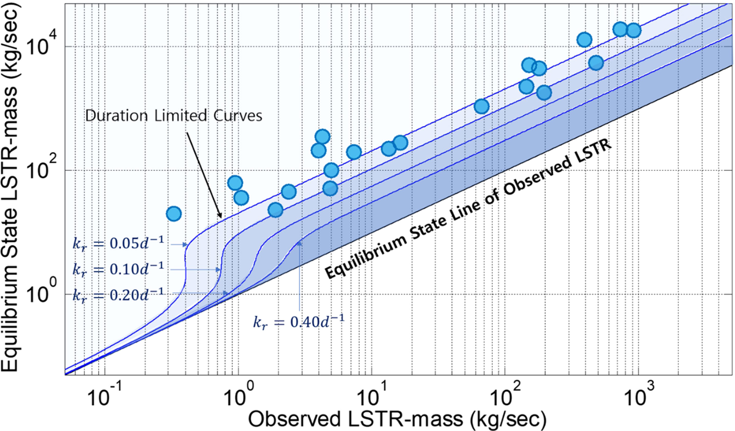
Figure 9 Comparison between LSTR-mass observation data and LSTR-mass values calculated by Eq. (34) according to the recovery factor.

The relationship is drawn based on the curve μ_p=1–exp(–k_rτ), where τ corresponding to the wave duration follows Eq. (38). Thus, if the y-axis of Figure 9 is a computed LSTR–mass in equilibrium state, this means that the data must lie on the right and upper sides of the curve shown according to the recovery factor. In addition, note that when comparing the computed and observed values, it may depend on the field wave condition at the time of measurement. That is, if the observation is recorded when the wave height is relatively small, wave heights with similar wave conditions are likely to occur consecutively; therefore, the wave duration can be regarded as long. However, if the observation is recorded during a storm wave event with a relatively large prevalent wave height, unlike the former, the wave duration can be regarded as extremely short; therefore, the observed data value is likely to be significantly smaller than the computed value.

7 Concluding remark

In this study, the horizontal behavior of suspended sediments due to storm incidence was applied to derive the governing equations of the shoreline change model. The model simulates shoreline changes due to suspended sediment moving alongshore, as well as the transverse suspension and recovery processes of beach sand. Applying the proposed governing equation to the equilibrium state yielded the same results as the existing shoreline change model. In the governing equation, the physical parameters, including the beach response and recovery factors, are obtained from the beach scale factor (Lim et al., 2022c). When introducing the DFLST, the littoral transport speed was obtained by applying longshore currents, as proposed by Bayram et al. (2007).

The DFLST was defined here as the ratio of littoral sediment transport speed to longshore wave-induced current and is similar to the transport coefficient introduced by Dean (1973) and Bayram et al. (2009) to estimate the LSTR of suspended sediment. The DFLST was estimated by comparison with the CERC (1984) formula and expressed as a function of the beach scale factor. However, in the future, a more accurate field investigation of the physical properties of DFLST should be conducted through multi-site observations of various beach conditions.

To verify the LSTR–mass proposed in this study, we compared it with the values obtained from existing observational data and empirical formulae. The empirical formulae used for comparison were the CERC (1984) formula, the Kamphuis (1991) formula, the Kamphuis (modified; Mil-Homens et al., 2013) formula, and the CROSMOR (van Rijn, 2014) formula. As a result, when the littoral transport speed obtained in this study was applied, it yielded the lowest error among all existing formulae, the log scale correlation was 0.969, and the RMSLE was 0.568. However, this comparison is only allowed based on the assumption that the sediment transport environment is regarded as an equilibrium state in which the time delay between wave and sediment concentration magnitudes is negligible and that events with a steady small wave height are maintained.

Kim et al. (2021) identified that when a storm wave occurs, a peak in the shoreline retreat occurs approximately one to two days after the peak wave height. Therefore, in a storm event, the wave heights given in the formula of LSTR and LSTR–mass have time delays between each other, unlike the equilibrium state. Thus, the correlation between wave duration and coastal energy flux by Van Wellen et al. (2000) showed that the rate of transport of coastal sediments obtained compared to the CERC formula is 20 times lower than the value required by the governance equation proposed in this paper.

It is expected that the shoreline change model proposed in this study will be highly applicable, unlike the existing shoreline change model, in which the sediments are suspended in the high wave influx; therefore, the shoreline retreats and the suspended sediments revert to their original positions. In addition, if the longshore wave-induced current is obtained from the numerical model, the littoral sediment speed given in the governing equation becomes the direct product of the calculated longshore wave-induced current $\overline{U_l}$ and the DFLST ϵ_L proposed in this study. Therefore, the governing equation proposed in this study is also useful for reproducing the rhythmic beach cusp formation caused by the difference in wave-induced current in the coastal direction.

Data availability statement

The original contributions presented in the study are included in the article/supplementary material. Further inquiries can be directed to the corresponding author.

Author contributions

Supervision, J-LL. Writing—original draft, CL. Writing—review and editing, CL, and J-LL. Data acquisition, CL. All authors contributed to the article and approved the submitted version.

Funding

This research was supported by the Korea Institute of Marine Science & Technology Promotion (KIMST), funded by the Ministry of Oceans and Fisheries, Korea (RS-2023-00256687).

Acknowledgments

John R. C. Hsu is acknowledged with gratitude for his comments aimed toward improving the manuscript.

Conflict of interest

CL and J-LL hold the patent for the Concept and Numerical Model.

Publisher’s note

All claims expressed in this article are solely those of the authors and do not necessarily represent those of their affiliated organizations, or those of the publisher, the editors and the reviewers. Any product that may be evaluated in this article, or claim that may be made by its manufacturer, is not guaranteed or endorsed by the publisher.

References

Bailard J. A., Jenkins S. A. (1984). “Systems for reducing sedimentation in berthing facilities,” in Dredging and dredged material disposal (Clearwater Beach, Florida, United State: ASCE), 311–320.

Google Scholar

Bayram A., Larson M., Hanson H. (2007). A new formula for the total longshore sediment transport rate. Coast. Eng. 54, 700–710.

Google Scholar

Bruno R. O., Dean R. G., Gable C. G. (1980). Littoral transport evaluations at a detached breakwater. Proceedings 17th Coast. Eng. Conf., 1453–1475.

Google Scholar

Chadwick A. J. (1989). Field measurements and numerical model verification of coastal shingle transport. Adv. Water modeling measurement (Cranfield), 387–402.

Google Scholar

CERC (1984). Shore protection manual. 4th Ed (Washington, D.C: U.S. Army Corps of Engineers, Waterways Experiment Station, Coastal Engineering Research Center, U.S. Government Printing Office).

Google Scholar

Coastal Engineering Manual (2002). Engineer manual 1110-2-1100 Vol. in 6 volumes) (Washington, DC: U.S. Army Corps of Engineers). Available at: http://www.usace.army.mil/inet/usace-docs/eng-manuals/cecw.htm.

Google Scholar

Dahl T. E., Stedman S. M. (2013). Status and trends of wetlands in the coastal watersheds of the conterminous united states 2004 to 2009 (U.S. Department of the Interior, Fish and Wildlife Service, and NOAA National Marine Fisheries Service), 46.

Google Scholar

Dean R. G. (1973). Heurisitic models of sand transport in the surf zone. Proceed. Eng. Dyn. Surf. Zone Sydney (Sydney, N.S.W.: Institution of Engineers, Australia), 208–214.

Google Scholar

Dean R. G. (1977). Equilibrium beach profiles: U.S. Atlantic and gulf coasts. technical report no. 12 (Delaware: Department of Civil Engineering, University of Delaware).

Google Scholar

Dean R. G., Berek E. P., Gable C. G., Seymour R. J. (1982). Longshore transport determined by an efficient trap. Proceedings 18th Int. Conf. Coast. Eng., 954–968.

Google Scholar

Dean R. G. (1989). Measuring longshore transport with traps. Nearshore Sediment Transport (New York), 313–336.

Google Scholar

Dean R. G., Dalrymple R. A. (2002). Coastal processes with engineering applications (United Kingdom: Cambridge University Press), 475.

Google Scholar

del Valle R., Medina R., Losada M. A. (1993). Dependence of coefficient K on grain size. J. Waterways Port Coastal Ocean Eng. ASCE 119 (5), 568–574. doi: 10.1061/(ASCE)0733-950X(1993)119:5(568)

CrossRef Full Text | Google Scholar

De Vriend H. J., Zyserman J., Nicholson J., Roelvink J. A., Pechon P., Southgate H. N. (1993). Medium-term 2DH coastal area modelling. Coastal Engineering 21, 193–224. doi: 10.1016/0378-3839(93)90050-I

CrossRef Full Text | Google Scholar

Floerl O., Atalah J., Bugnot A. B., et al. (2021). A global model to forecast coastal hardening and mitigate associated socioecological risks. Nat. Sustain. 4, 1060–1067. doi: 10.1038/s41893-021-00780-w

CrossRef Full Text | Google Scholar

Foley M. M., Jonathan A. W., Andrew R., Andrew W. S., Patrick B. S., Jeffrey J. D., et al. (2017). Coastal habitat and biological community response to dam removal on the elwha river. Ecol. Monogr. 87, 552–577. doi: 10.1002/ecm.1268

CrossRef Full Text | Google Scholar

French J., Payo A., Murray B., Orford J., Eliot M., Cowell P. (2016). Appropriate complexity for the prediction of coastal and estuarine geomorphic behaviour at decadal to centennial scales. Geomorphology 256, 3–16. doi: 10.1016/j.geomorph.2015.10.005

CrossRef Full Text | Google Scholar

Gable C. G. (1981). Report on data from NSTS experiments at leadbetter beach, Santa Barbara, California (Santa Barbara, California: University of California, Institute of Marine Resources, Rep., No. 80-5).

Google Scholar

González M., Medina R., Losada M. (2010). On the design of beach nourishment projects using static equilibrium concepts: application to the Spanish coast. Coast. Eng. Special Issue 57 (2), 227–240. doi: 10.1016/j.coastaleng.2009.10.009

CrossRef Full Text | Google Scholar

Hanson G. J. (1990). Surface erodibility of earthern channels at high stresses. part I - open channel testing. Trans. Am. Soc Agric. Engineer 33, 0127–0131. doi: 10.13031/2013.31305

CrossRef Full Text | Google Scholar

Hanson G. J. (1997). And cook, K Development of excess shear stress parameters for circular jet testing. R. Proc. Am. Soc. Agric. Engineers ASCE (Minneapolis, USA).

Google Scholar

Hsu J. R. C., Uda T., Silvester R. (2000). “Shoreline protection methods–Japanese experience,” in Handbook of coastal engineering. Ed. Herbich J. B. (New York: McGraw-Hill), 9.1–9.77.

Google Scholar

Ingle J. C. (1966). The movement of beach sand (New York: Elsevier), 221 pp.

Google Scholar

Inman D. L., Bagnold R. A. (1963). “Littoral processes,” in The Sea, vol. 3 . Ed. Hill M. N. (New York: Interscience), 529–533.

Google Scholar

Kamphuis J. W. (1991). Alongshore sediment transport rate. J. Waterways Port Coast. Ocean Eng. ASCE 117 (6), 624–640. doi: 10.1061/(ASCE)0733-950X(1991)117:6(624)

CrossRef Full Text | Google Scholar

Kamphuis J. W., Davies M. H., Nairn R. B., Sayao O. J. (1986). Calculation of littoral sand transport rate. Coast. Eng. 10 (1), 1–21. doi: 10.1016/0378-3839(86)90036-0

CrossRef Full Text | Google Scholar

Kana T. W.. (1977). Suspended sediment transport at prince inlet. proc. coastal Sediments’77 (ASCE), 1069–1088.

Google Scholar

Kana T. W., Ward L. G. (1980). Nearshore suspended sediment load during storm and post-storm conditions. Coast. Eng. (Sydney, Australia), 1158–1174. doi: 10.1061/9780872622647.071

CrossRef Full Text | Google Scholar

Kim T. K., Lim C., Lee J. L. (2021). Vulnerability analysis of episodic beach erosion by applying storm wave scenarios to a shoreline response model. Front. Mar. Sci. 8. doi: 10.3389/fmars.2021.759067

CrossRef Full Text | Google Scholar

Komar P. D., Inman D. L. (1970). Longshore sand transport on beaches. J. Geophys. Res. 75 (30), 5514–5527. doi: 10.1029/JC075i030p05914

CrossRef Full Text | Google Scholar

Komar P. D. (1988). Environmental controls on littoral sand transport. Proc. 21st Int. Conf. Coast. Eng., 1238–1252.

Google Scholar

Kraus N. C., Dean J. L. (1987). Longshore sediment transport rate distributions measured by trap. proc. coastal Sediments’87 (New Orleans, USA: ASCE), 881–896.

Google Scholar

Larson M., Kraus N. (1991). Numerical model of longshore current for bar and trough beaches. J. Waterway Port Coast. Ocean Eng. 117 (4), 326–347.

Google Scholar

Lee K. K. (1975). Longshore currents and sediment transport in West shore of lake Michigan. Water Resour. Res. 11 (6), 1029–1032. doi: 10.1029/WR011i006p01029

CrossRef Full Text | Google Scholar

Lee J. L., Hsu J. R. C. (2017). “Numerical simulation of dynamic shoreline changes behind a detached breakwater by using an equilibrium formula,” in Proceedings of the International Conference on Offshore Mechanics and Arctic Engineering (Trondheim, Norway), Trondheim, Norway. 25–30.

Google Scholar

Lee S., Lee J. L. (2020). Estimation of background erosion rate at janghang beach due to the construction of geum estuary tidal barrier in Korea. J. Mar. Sci. Eng. 8, 551. doi: 10.3390/jmse8080551

CrossRef Full Text | Google Scholar

Lim C., Hsu J. R. C., Lee J. L. (2022a). MeePaSoL: a MATLAB-based GUI software tool for shoreline management. Comput. Geosci. 161, 105059. doi: 10.1016/j.cageo.2022.105059

CrossRef Full Text | Google Scholar

Lim C., Kim T. K., Lee J. L. (2022b). Evolution model of shoreline position on sandy, wave-dominated beaches. Geomorphology 415 (15), 108409. doi: 10.1016/j.geomorph.2022.108409

CrossRef Full Text | Google Scholar

Lim C., Kim T.-K., Kim J.-B., Lee J.-L. (2022c). A study on the influence of sand median grain size on the short-term recovery process of shorelines. Front. Mar. Sci. 9. doi: 10.3389/fmars.2022.906209

PubMed Abstract | CrossRef Full Text | Google Scholar

Lim C., Kim T. -K., Lee S., Yeon Y. J., Lee J. L. (2021). Assessment of potential beach erosion risk and impact of coastal zone development: a case study on bongpo–cheonjin beach. Nat. Hazard Earth Syst. Sci. 21, 3827–3842. doi: 10.5194/nhess-21-3827-2021

CrossRef Full Text | Google Scholar

Mil-Homens J., Ranasinghe R., van Thiel de Vries J. S. M., Stive M. J. F. (2013). Re-evaluation and improvement of three commonly used bulk longshore sediment transport formulae. Coast. Eng. 75, 29–39. doi: 10.1016/j.coastaleng.2013.01.004

CrossRef Full Text | Google Scholar

Miller H. C. (1999). Field measurements of longshore sediment transport during storms. Coast. Eng. 36, 301–321. doi: 10.1016/S0378-3839(99)00010-1

CrossRef Full Text | Google Scholar

Miller J. K., Dean R. G. (2004). A simple new shoreline change model. Coast. Eng. 51, 531–556. doi: 10.1016/j.coastaleng.2004.05.006

CrossRef Full Text | Google Scholar

Ministry of Oceans and Fisheries (2020). Development of coastal erosion control technology (Sejong, South Korea: Ministry of Oceans and Fisheries R&D Report).

Google Scholar

Montaño J., Coco G., Antolínez J. A. A., Beuzen T., Bryan K. R., Cagigal L., et al. (2020). Blind testing of shoreline evolution models. Scient. Rep. 10, 2137. doi: 10.1038/s41598-020-59018-y

CrossRef Full Text | Google Scholar

Moore G. W., Cole J. Y. (1960). “Coastal processes in the vicinity of cape Thompson, Alaska,” in Geologic investigations in support project chariot in the vicinity of cape Thompson, northwestern Alaska (USA: U.S. Department of Interior, Geological Survey).

Google Scholar

Nicholls R. J., Webber N. B. (1987). Aluminum pebble tracer experiments on Hurst castle spit. Proceedings Coast. Sediments ’87 (New Orleans), 1563–1577, ASCE.

Google Scholar

Partheniades E. (1965). Erosion and deposition of cohesive soils. J. Hydraul. Div-ASCE 91 (1), 105–139. doi: 10.1061/JYCEAJ.0001165

CrossRef Full Text | Google Scholar

Pelnard-Considère R. (1956). Essai de théorie de l’évolution des formes de rivage en plages de sable et de galets. 4th Journées l’Hydraulique Repport No. 1, 289–298.

Google Scholar

Ranasinghe R. (2016). Assessing climate change impacts on open sandy coasts: a review. Earth Sci. Rev. 160, 320–332. doi: 10.1016/j.earscirev.2016.07.011

CrossRef Full Text | Google Scholar

Reeve D., Chadwick A., Fleming C. (2012). Coastal engineering: processes, theory and design practice. 2nd Ed (London: Spon Press, Taylors & Francis), 514 pp.

Google Scholar

Roelvink D., Reniers A. J. H. M., Van Dongeren A., Van Thiel de Vries J., Lescinski J., McCall R. (2010). XBeach model description and manual (Delft, Netherlands: Unesco-IHE Institute for Water Education, Deltares and Delft University of Technology).

Google Scholar

Roelvink J. A., Van Banning G. K. F. M. (1995). Design and development of DELFT3D and application to coastal morphodynamics, oceanogr. Lit. Rev. 11 (42), 925.

Google Scholar

Samaras A. G., Koutitas C. G. (2014). Modeling the impact of climate change on sediment transport and morphology in coupled watershed-coast systems: a case study using an integrated approach. J. Sediment Res. 29 (3), 304–315. doi: 10.1016/S1001-6279(14)60046-9

CrossRef Full Text | Google Scholar

Schoonees J. S., Theron A. K. (1993). Review of the field-data base for longshore sediment transport. Coast. Eng. 19, 1–25. doi: 10.1016/0378-3839(93)90017-3

CrossRef Full Text | Google Scholar

Schoonees J. S., Theron A. K. (1996). Improvement of the most accurate longshore transport formula. proc. 25th Int.Conf. coastal eng (Orlando, USA: ASCE).

Google Scholar

Stive M. J. F., Aarninkhof S. G. J., Hamm L., Hanson H., Larson M., Wijnberg K. M., et al. (2002). Variability of shore and shoreline evolution. Coast. Eng. 47, 211–235. doi: 10.1016/S0378-3839(02)00126-6

CrossRef Full Text | Google Scholar

Stive M. J. F., Ranasinghe R., Cowell P. (2009). “Sea Level rise and coastal erosion,” in Handbook of coastal and ocean engineering. Ed. Kim Y. (Singapore: World Scientific), 1023–1038. doi: 10.1142/9789812819307_0037

CrossRef Full Text | Google Scholar

Swart D. H. (1976). Predictive equations regarding coastal transports. Proc. 15th Coast. Eng. Conf., 1113–1132.

Google Scholar

van Rijn L. C. (2002). Longshore transport. proc. 28th Int.Conf. coastal eng (Cardiff: ASCE), 2439–2451.

Google Scholar

van Rijn L. C. (2014). A simple general expression for longshore transport of sand, gravel and shingle. Coast. Eng. 90, 23–39. doi: 10.1016/j.coastaleng.2014.04.008

CrossRef Full Text | Google Scholar

Van Wellen E., Chadwick A. J., Mason T. (2000). A review and assessment of longshore sediment transport equations for coarse-grained beaches. Coast. Eng. 40, 243–275.

Google Scholar

Vitousek S., Barnard P. L., Limber P., Erikson L., Cole B. (2017). A model integrating longshore and cross-shore processes for predicting long-term shoreline response to climate change. J. Geophys. Res. Earth Surf. 122, 782–806. doi: 10.1002/2016JF004065

CrossRef Full Text | Google Scholar

Walton T., Chiu T. (1979). A review of analytical techniques to solve the sand transport equation and some simplified solutions. Proc. Coast. Structures 79, 809–837.

Google Scholar

Wang P., Kraus N. C. (1999). Longshore sediment transport rate measured by short-term impoundment. J. Waterways Port Coastal Ocean Eng. ASCE 125 (3), 118–126. doi: 10.1061/(ASCE)0733-950X(1999)125:3(118).

CrossRef Full Text | Google Scholar

Wang P., Kraus N. C., Davis R. A. (1998). Total longshore transport rate in the surf zone; field measurements and empirical prediction. J. Coast. Res. 14 (1), 2690282.

Google Scholar

Warner J. C., Armstrong B., He R., Zambon J. B. (2010). Development of a coupled ocean–atmosphere–wave–sediment transport (COAWST) modeling system. Ocean Model. 35 (3), 230–244. doi: 10.1016/j.ocemod.2010.07.010

CrossRef Full Text | Google Scholar

Warrick J. A., Stevens A. W., Miller I. M., Harrison S. R., Ritchie A. C., Gelfenbaum G. (2019). World’s largest dam removal reverses coastal erosion. Sci. Rep. 9, 1–12. doi: 10.1038/s41598-019-50387-7

PubMed Abstract | CrossRef Full Text | Google Scholar

Watts G. M. (1953). A study of sand movement at south lake worth inlet Florida (Vicksburg: Coastal Engineering Research Center).

Google Scholar

Wright L. D., Short A. D., Green M. O. (1985). Short-term changes in the morphodynamic states of beaches and surf zones: an empirical predictive model. Mar. Geol. 62, 339–364. doi: 10.1016/0025-3227(85)90123-9

CrossRef Full Text | Google Scholar

Yates M. L., Guza R. T., O’Reilly W. C. (2009). Equilibrium shoreline response: observations and modeling. J. Geophys. Res. 114 (C9), 116. doi: 10.1029/2009JC005359

CrossRef Full Text | Google Scholar