Simulated and projected SST of Asian marginal seas based on CMIP6 models

Jin, Shanshan; Wei, Zexun; Wang, Dingqi; Xu, Tengfei

doi:10.3389/fmars.2023.1178974

ORIGINAL RESEARCH article

Front. Mar. Sci., 28 July 2023

Sec. Global Change and the Future Ocean

Volume 10 - 2023 | https://doi.org/10.3389/fmars.2023.1178974

Simulated and projected SST of Asian marginal seas based on CMIP6 models

Shanshan Jin¹

Zexun Wei^2,3

Dingqi Wang^2,3

Tengfei Xu^2,3*

¹College of Meteorology and Oceanography, National University of Defense Technology, Changsha, China
²First Institute of Oceanography, and Key Laboratory of Marine Science and Numerical Modeling, Ministry of Natural Resources, Qingdao, China
³Laboratory for Regional Oceanography and Numerical Modeling, Pilot National Laboratory for Marine Science and Technology, Qingdao, China

Sea surface temperature (SST) is an important element in studying the global ocean-atmospheric system, as well as its simulation and projection in climate models. In this study, we evaluate the simulation skill of the Coupled Model Intercomparison Project Phase 6 (CMIP6) models in simulating the climatological SST in the Asian Marginal Seas (AMS), known as the most rapidly warming region over the global ocean. The results show that the spatial patterns and seasonal variability of Asian Marginal Seas (AMS) climatological SST simulated by the CMIP6 models are generally in good agreement with the observations, but there are simulation biases in the values. In boreal winter, the simulated climatological SST tends to be overestimated in the Japan/East Sea and the East China Seas (ECSs) by up to 2°C, while being underestimated in the Sea of Okhotsk by up to 2°C. In boreal summer, the simulated climatological SSTs are overestimated in the Indonesian seas and western Arabian Sea, while being underestimated in the Sea of Okhotsk and the northern ECSs by 1.2–1.5 and 2°C, respectively. Furthermore, we calculate the projected sea surface warming trends in the AMS under different future scenarios in the CMIP6 models. The results show warming trends of 0.8–1.8, 1.7–3.4, and 3.8–6.5°C/century for the Shared Socio-Economic Pathway (SSP) of low- (global radiative forcing of 2.6 W/m² by the year 2100), medium- (global radiative forcing of 4.5 W/m² by 2100) and high-end (8.5 W/m² by 2100) pathways, respectively. In addition, the middle and high latitudes of the AMS are found to have faster warming trends than the low latitudes, with the most rapidly warming occurring in the Sea of Okhotsk, which is around 2 times larger than the global mean SST warming trend. The SST warming trends are relatively slow in the South China Sea and the Indonesian seas, roughly equal to the global mean SST warming trend.

1 Introduction

Sea surface temperature (SST) is a fundamentally important variable for revealing the state of the ocean. It is a critical determinant of climate variability through air-sea interaction, e.g., the exchange of heat, momentum, and moisture between the ocean and the atmosphere (Wentz et al., 2000; Wang et al., 2011). The onset of an El Niño-Southern Oscillation (ENSO) event is induced by the coupling of SST to the Walker Circulation, namely, the Bjerknes feedback (Bjerknes, 1969). The ENSO phenomenon and its rainfall response are suggested to be significantly changed under anthropogenic warming (Santoso et al., 2013; Cai et al., 2015; Cai et al., 2021). The Indian Ocean Dipole (IOD) and corresponding rainfall pattern are also related to the coupling of SST to the atmospheric circulation (Saji et al., 1999). A warm SST background is also the necessary condition for the development of tropical cyclone and hurricane, and strongly influences their evolution and trajectory (Sun et al., 2022). A cold SST anomaly is often associated with upwelling and thus benefits to nutrient concentration and primary productivity (Barale, 2018). Moreover, SST is one of the most readily measurable variables of the ocean, which has an accumulation of records more than hundred years. Therefore, SST records are widely used as indictors for climate modes (e.g., ENSO, IOD, Pacific Decadal Oscillation, Atlantic Multidecadal Oscillation). The SST could impact rainfall pattern over the land by modulating the atmospheric circulation and moisture transport, thereby affecting crop yields or even inducing drought and/or flood disasters (Gaetani et al., 2017; Karan et al., 2022).

The Asian Marginal Seas (AMS), which extend from the near-polar to the near-equatorial regions and span most of the climatic zones of the Earth, affecting the largest amount of population in the world, and are probably to be the most heavily impacted by anthropogenic activities (Barale, 2018; Nam et al., 2022). The AMS SST plays an important role in modulating the Asian monsoon system (Li et al., 2010; Yi and Yeh, 2019), thereby impacting on the socioeconomic conditions of the Asian countries with large populations located around the coast of the AMS. In addition, the AMS are also known as one of the major distribution regions of coral reefs, mangroves, and fishery (Spalding et al., 2001; Giri et al., 2011; Veron et al., 2015; Bai et al., 2018).

It is important noting that the AMS is one of the most rapidly warming regions over the global oceans (Belkin, 2009; Lima and Wethey, 2012; Wu et al., 2012; Bao and Ren, 2014; Wang et al., 2016). For example, the warming trends of boreal winter SST in the ECS and the Taiwan Strait exceed 2.7°C per hundred years (Liu and Zhang, 2013), about two times larger than the global mean SST trend (Sasaki and Umeda, 2021). The dynamics could attribute to increasing oceanic heat advection, acceleration of the Kuroshio, local atmospheric forcing, and a weakening East Asian monsoon (Yeh and Kim, 2010; Seo et al., 2014; Cai et al., 2017; Yi and Yeh, 2019; Sasaki and Umeda, 2021; Wang and Wu, 2022).

SST variability in the marginal seas has a substantial influence on regional climate change (Xie et al., 2002; Xu et al., 2011; Miyama et al., 2012; Sasaki and Umeda, 2021). In the Arabian Sea, the SST is closely related to the monsoon rainfall in both winter and summer (Levine and Turner, 2012; Levine et al., 2013; Fathrio et al., 2017). The future warming of SST in the ECS could increase the frequency of torrential rainfall events over western Japan (Manda et al., 2014).Therefore, understanding the distribution of AMS SST and its projected trends is important for ocean and climate studies (Meng et al., 2022; Sun et al., 2022), and for the sustainable development strategy in the seas of East Asia (PEMSEA (Partnerships in Environmental Management for the Seas of East Asia), 2003).

Numerical ocean, climate and earth system models are important tools for understanding and predicting SST, and accordingly, simulation skill of SST is one of the most important indicators for model assessment (Fischer et al., 2018; Yang et al., 2018). Around 20 years ago, the World Climate Research Programme’s (WCRP) Working Group on Coupled Modelling (WGCM) has proposed the Coupled Model Intercomparison Project (CMIP), with a specific focus on better understanding and prediction for climate change, and is served as the main database for the Assessment Report of the Intergovernmental Panel on Climate Change (IPCC) (Meehl et al., 1997; Meehl et al., 2000; Meehl et al., 2007; Taylor et al., 2012; Eyring et al., 2016). Now, the phase 6 of the CMIP (CMIP6) is finalized, with a total of more than 70 models from 33 institutions (Eyring et al., 2016). Compared to the previous phase 5 of the CMIP (CMIP5) models, the CMIP6 models show improvements in the SST simulation. For example, the excessive westward extension biases of the equatorial Pacific cold tongue in the CMIP5 models (Li and Xie, 2012; Li and Xie, 2014) have been reduced in CMIP6 models (Jiang et al., 2021). Biases in the western equatorial Indian Ocean, and in the subtropical and tropical Pacific and Atlantic oceans have been reduced in the CMIP6 models (Fathrio et al., 2017; Li et al., 2022). Unrealistic patterns of interannual and decadal SST variations as well as long-term SST trends have also been improved (Jha et al., 2014; Halder et al., 2022).

Most of existed assessment on the SST simulation in climate models only focus on open oceans (Ham and Kug, 2015; Fathrio et al., 2017; Borchert et al., 2021), with less attention on the SST in the AMS. In this study, we will assess the AMS SST simulation skill in the CMIP6 climate models by comparing with observation, and to exhibit the projected AMS SST based on the CMIP6 future scenario experiments. The uncertainty of the projected AMS SST will also be discussed. The data and methods used in this study are introduced in Section 2. In Section 3, we analyze the SST bias of the CMIP6 models in AMS in comparison to the observations. The evaluation of the SST bias is an important step in reducing bias in future climate model development. Section 4 shows the SST trend based on projected simulation under three Shared Socioeconomic Pathway (SSP) scenarios. Discussion and conclusions are given in Section 5 and Section 6, respectively.

2 Data and methods

2.1 Data

2.1.1 Observations

The Hadley Centre Global Sea Ice and Sea Surface Temperature (HadISST) provides the observed monthly SST from 1871 to the present, with a horizontal resolution of 1°×1°. The HadISST uses reduced space optimal interpolation applied to SSTs from the Marine Data Bank (mainly ship tracks) and ICOADS through 1981 and a blend of in-situ and adjusted satellite-derived SSTs for 1982-onwards (Rayner et al., 2003). In this study, we used the data from 1871 to 2014. The AMS are divided as the Bering Sea (region A), the Sea of Okhotsk (region B), the Japan/East Sea (JES) (region C), the East China Seas (includes the East China Sea, the Yellow Sea and the Bohai Sea, ECSs) (region D), the Philippine Sea (region E), the South China Sea (SCS) (region F), the Indonesian seas (region G), the Bay of Bengal (region H), and the Arabian Sea (region I), according to the geography surrounding the Asia continent (Figure 1).

FIGURE 1

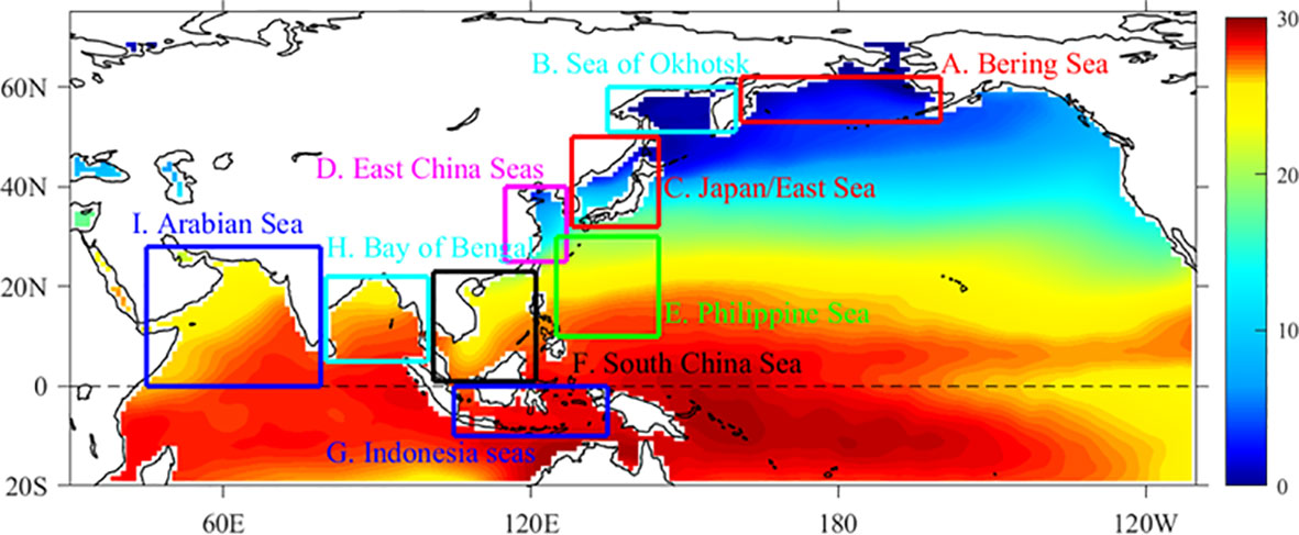
Figure 1 Study regions of the Asian Marginal Seas (AMS), with background color map representing the distribution of the climatological sea surface temperature based on the observation from 1871 to 2014. The boxes indicate A. Bering Sea (160°E–160°W, 53°N–62°N); B. Sea of Okhotsk (135°E–157°E, 51°N–60°N); C. Japan/East Sea (128°E–142°E, 32°N–50°N); D. East China Seas (includes the East China Sea, the Yellow Sea and the Bohai Sea, ECSs; 117°E–127°E, 25°N–42°N); E. Philippine Sea (125°E–145°E, 10°N–30°N); F. South China Sea (SCS; 105°E–121°E, 0°–23°N); G. Indonesian seas (105°E–135°E, 10°S–0°); H. Bay of Bengal (80°E–100°E, 5°N–22°N); I. Arabian Sea (45°E–77°E, 0°–28°N).

2.1.2 CMIP6 models

In this study, we use the historical simulation and future scenarios outputs to provide an overall assessment of the simulation skill and projected changes of the AMS SST in the CMIP6 models, respectively. The historical simulation is the benchmark experiment of the CMIP6 models, forced by both natural (e.g., solar variability and volcanic aerosols) and anthropogenic factors (e.g., CO₂ concentration, aerosols) since the Industrial Revolution (1850–2014). Three future scenario simulations under Shared Socio-Economic Pathway (SSP) of low- (global radiative forcing of 2.6 W/m² by the year 2100), medium- (global radiative forcing of 4.5 W/m² by 2100) and high-end (8.5 W/m² by 2100) pathways, namely, the SSP126, SSP245, and SSP585, provide the projected SST changes for future periods (2015–2100). Details of the configuration of the CMIP6 historical and scenario simulations are given in Eyring et al. (2016) and Riahi et al. (2017). Historical simulations from 41 models, SSP126 and SSP245 simulations from 26 models, and SSP585 simulations from 27 models in the CMIP6 were considered (Table 1). For simplicity, we analyzed only one mean member, the “r1i1p1f1” of the CMIP6 historical outputs. The monthly mean outputs of these CMIP6 models were interpolated horizontally onto a 1° × 1° regular longitude-latitude grid using linear interpolation before analysis.

TABLE 1

Table 1 Details of models used in CMIP6 analysis of Asia Marginal Seas (AMS).

2.2 Methods

2.2.1 Taylor diagram and TD score

A Taylor diagram provides a concise statistical summary for evaluating the simulation of SST by indicating how closely a pattern matches observations (Taylor, 2001). Given the simulated and observed SSTs as “model” field (M) and “reference” filed (O), the Taylor diagram represents the spatial correlation coefficient (R), the centered root-mean-square (RMS) error E’ between M and O, and spatial standard deviation of the “model” field (σ_M) and “reference” field (σ_O) as a single point, with the observed SST as reference point. They are calculated as follows:

R = \frac{\frac{1}{N} \sum_{n = 1}^{N} (M_{n} - \bar{M}) (O_{n} - \bar{O})}{σ_{M} σ_{O}}

σ_{M} = \sqrt{\frac{1}{N} \sum_{n = 1}^{N} {(M_{n} - \bar{M})}^{2}}

σ_{O} = \sqrt{\frac{1}{N} \sum_{n = 1}^{N} {(O_{n} - \bar{O})}^{2}}

E' = \sqrt{\frac{1}{N} \sum_{n = 1}^{N} {[(M_{n} - \bar{M}) - (O_{n} - \bar{O})]}^{2}}

where M_n and O_n are the values of “model” and “reference” fields at each grid point, respectively; and N is the total grid point number of the field, the overbar indicates the overall mean of a field. The relationship between three values satisfies the Law of Cosines. Since different fields use different units of measurement, their statistics must be nondimensionalized before being displayed on the same graph. Therefore, E’, σ_M, and σ_O are normalized by dividing σ_O, so as to make the reference point at (R=1, σ_O=1).

\hat{E'} = E' / σ_{O}, {\hat{σ}}_{M} = σ_{M} / σ_{O}, a n d {\hat{σ}}_{O} = 1

The Taylor Diagram Score (TD) is used to quantify the similarity between the simulated and observed SST, with smaller TD value implying better simulation skill.

T D = | 1 - R | + | 1 - \frac{σ_{M}}{σ_{O}} | + \frac{E'}{σ_{O}}

where R, σ and $E'$ have the same meaning as in the previous formulae.

The SST warming trend is calculated based on linear fitting. For a certain latitude and longitude point, the first-order coefficient obtained by one-dimensional linear fitting of SST time series is its trend. For example, when calculating the trend of latitude and longitude points (lon, lat) in January, the first step is to obtain the SST time series SSTy={SST1, SST2, SST3,…, SSTn} of that latitude and longitude point in January each year. Then, a one-dimensional linear fitting SSTy=kx+b is performed, k is the trend of that point in January, and its unit is °C/year.

2.2.2 Causation analysis

The causality is measured by the rate of information flows from one series to the next. The causality analysis can provide timely help with research in climate science, an example is the cause-and -effect relationship between two climate modes, El Niño and the Indian Ocean Dipole (IOD). The information flow is used to measure the causation between dynamical events, in order to quantitatively analyze the causality (Liang, 2014). For given two time series, the quantitative causal relation between the series will be obtained by causality analysis. The information flow is used to measure the causation. It can tell not only the magnitude of information exchange but also the direction of the cause-effect relationship.

For time series X₁ and X₂, the rate of information flows (units: nats per unit time) from the latter to the former is:

T_{2 \to 1} = \frac{C_{11} C_{12} C_{2, d 1} - C_{12}^{2} C_{1, d 1}}{C_{11}^{2} C_{22} - C_{11} C_{12}^{2}}

where C_ij is the sample covariance between X_i and X_j, C_i,dj is the covariance between X_i and $\dot{X_{j}}$ , and $\dot{X_{j}}$ is the difference approximation of $d X_{j} / d t$ using the Euler forward scheme:

{\dot{X}}_{j, n} = \frac{X_{j, n + k} - X_{j, n}}{k Δ t}

If $T_{2 \to 1} = 0$ , X₂ does not cause X₁; if not, it is causal. The magnitude of the value indicates the strength of the causality.

3 Assessment of the simulation skill of SST by the CMIP6 models

In observation, the climatological SST is basically getting colder with increased latitudes both in January and July (Figures 2A, B). The SST in the northern Arabian Sea, northern Bay of Bengal, SCS, Indonesian seas, and Philippine Sea is below 28°C in boreal winter (January), whereas it increases in boreal summer (July). The seasonal variation of the AMS climatological SST shows a larger seasonal variation exceeding 10°C in the middle latitudes (e.g., the ECSs and the JES), whereas a smaller seasonal variation of less than 4°C is found in the tropical marginal seas (e.g., the Philippine Sea, SCS, Indonesian seas, Bay of Bengal, and Arabian Sea) (Figure 2C). The simulated AMS climatological SST generally shows similar patterns in boreal winter and summer, as well as seasonal variation, as revealed by the comparison between the multi-model ensemble means (MME) of CMIP6 models and the observation (Figures 2D–F).

FIGURE 2

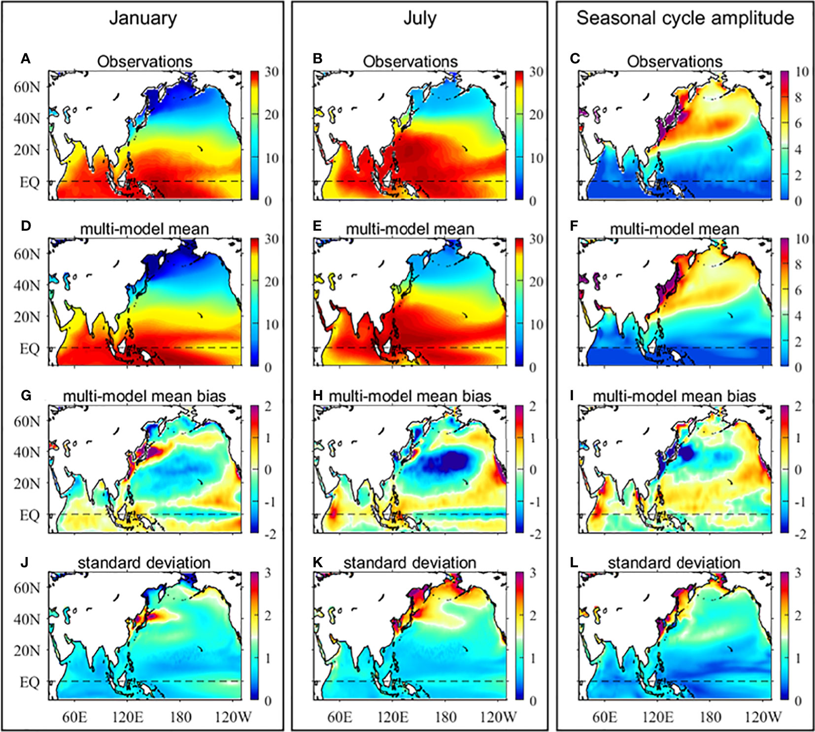
Figure 2 Observed and simulated climatological sea surface temperature (SST) in boreal winter (left column) and summer (middle column), and seasonal variation (right column). (A–C) HadISST; (D–F) multi-model ensemble mean (MME) of the CMIP6 models; (G–I). biases between the CMIP6 MME and HadISST; (J–L) cross-model standard deviation of the simulated climatological SST in the CMIP6 models.

Figures 2G–I show the biases of the AMS climatological SST between the CMIP6 MME and observation. For the simulation of climatological SST, the area below the significance level is found in the northwest Sea of Okhotsk in January. In boreal winter, the largest positive and negative biases occur in the JES and the ECSs, with values up to 2°C, and in the Sea of Okhotsk (up to −2°C), respectively (Figure 2G). Additionally, the winter climatological SSTs are overestimated in the SCS, the northern Bay of Bengal, and the Indonesian seas, whereas they are underestimated in the Bering Sea, Arabian Sea, and the Philippine Sea, but with relatively smaller biases of approximately 0.5°C in most areas (Figure 2G). In boreal summer, the largest positive biases occur in the Indonesian seas and along the west coast of Africa in the Arabian Sea, with values approximately of 1.2−1.5°C, and the largest negative biases occur in the Sea of Okhotsk, the Bohai Sea, and the northern ECS (exceeding −2°C) (Figure 2H). It can be seen that the CMIP6 models tend to produce warmer SST in the JES and ECSs in boreal winter, whereas they produce colder SST in boreal summer (Figures 2G, H). Consequently, the amplitudes of seasonal variations are underestimated by more than 3°C in the JES and ECSs (Figure 2I). On the contrary, the amplitudes of seasonal variations are overestimated along the north coast of the Sea of Okhotsk, the western Arabian Sea, the eastern Bay of Bengal, and the Philippine Sea, with the largest positive biases of approximately 2°C occurring in the western Arabian Sea and the eastern Bay of Bengal (Figure 2I).

Yi and Yeh (2019) pointed out that the East AMS SST bias is related to atmospheric teleconnections from the tropical to the western-to-central North Pacific. The East AMS SST bias is also associated with the bifurcation latitude of the North Equatorial Current, a low bifurcation latitude transports more warm water into the East AMS (Yi and Yeh, 2019). In the Arabian Sea, a clear relationship exists between cold SST bias and weak monsoon rainfall in CMIP5 models during winter (Levine and Turner, 2012; Levine et al., 2013). In addition, the climatological SST bias in the Northeast Pacific is mainly attributed to the surface cloud radiative, clear-sky surface downward shortwave and longwave radiation, and surface albedo feedback (Zhang et al., 2023). Among the CMIP6 models, the discrepancies in the simulated AMS climatological SST are found occurring in the JES in boreal winter, and in the eastern Bering Sea, the Sea of Okhotsk, the western JES, and the northern ECSs in boreal summer, rather than in other regions (Figures 2J, K). As a result, the cross-model standard deviation of the seasonal variation shares a similar pattern as that of the climatological SST in boreal summer (Figure 2L).

Figure 3 shows the Taylor diagram of the simulated AMS climatological SST in boreal winter in the CMIP6 models. The observed climatological SSTs are represented by the blue pentagram, located on the point with R=1, σ=1, and E’=0. Generally, the closer the simulation points to the observation point, the better the simulation is, in comparison with the observation. The grid points of each AMS are 255, 90, 45, 48, 341, 165, 92, 180, and 426 from region A to region I, respectively. The correlation coefficients between observed SST and simulated SST pass the 95% confidence test, if correlation coefficients exceeding 0.13, 0.21, 0.29, 0.28, 0.11, 0.15, 0.21, 0.15, and 0.10 in regions A – I, respectively. In boreal winter, the “worst” simulation occurs in the Sea of Okhotsk, as revealed by its smallest correlation (R< 0.6 in most of the models), widely spread spatial standard deviation (0.25< σ< 4), and largest centered RMS error (E’ > 1 in most of the models and up to 3) (Figure 3B). The CMIP6 models show the “best” simulation of climatological SST in the Philippine Sea, with R > 0.97, 0.7< σ< 1.3, and E’< 0.4 (Figure 3E). In addition, there are also high spatial correlations (R > 0.9) above the 99% significance level in the JES, ECSs, SCS, and Arabian Sea, suggesting the boreal winter climatological SST patterns in these regional seas are well reproduced by the CMIP6 models (Figures 3C, D, F, I). In comparison, the model points are scattered in the Bering Sea, Indonesian seas, and the Bay of Bengal, indicating that the climatological SST simulation in these regions has a large difference among the CMIP6 models (Figures 3A, G, H). The Indonesian seas are subject to strong and complicate tidal mixing, which is not appropriate considered in most of existed models (Wen et al., 2021). Consequently, the simulated climatological SST shows large uncertainty in the CMIP6 models, e.g., with a wide range of correlation of −0.07< R< 0.9 (Figure 3G).

FIGURE 3

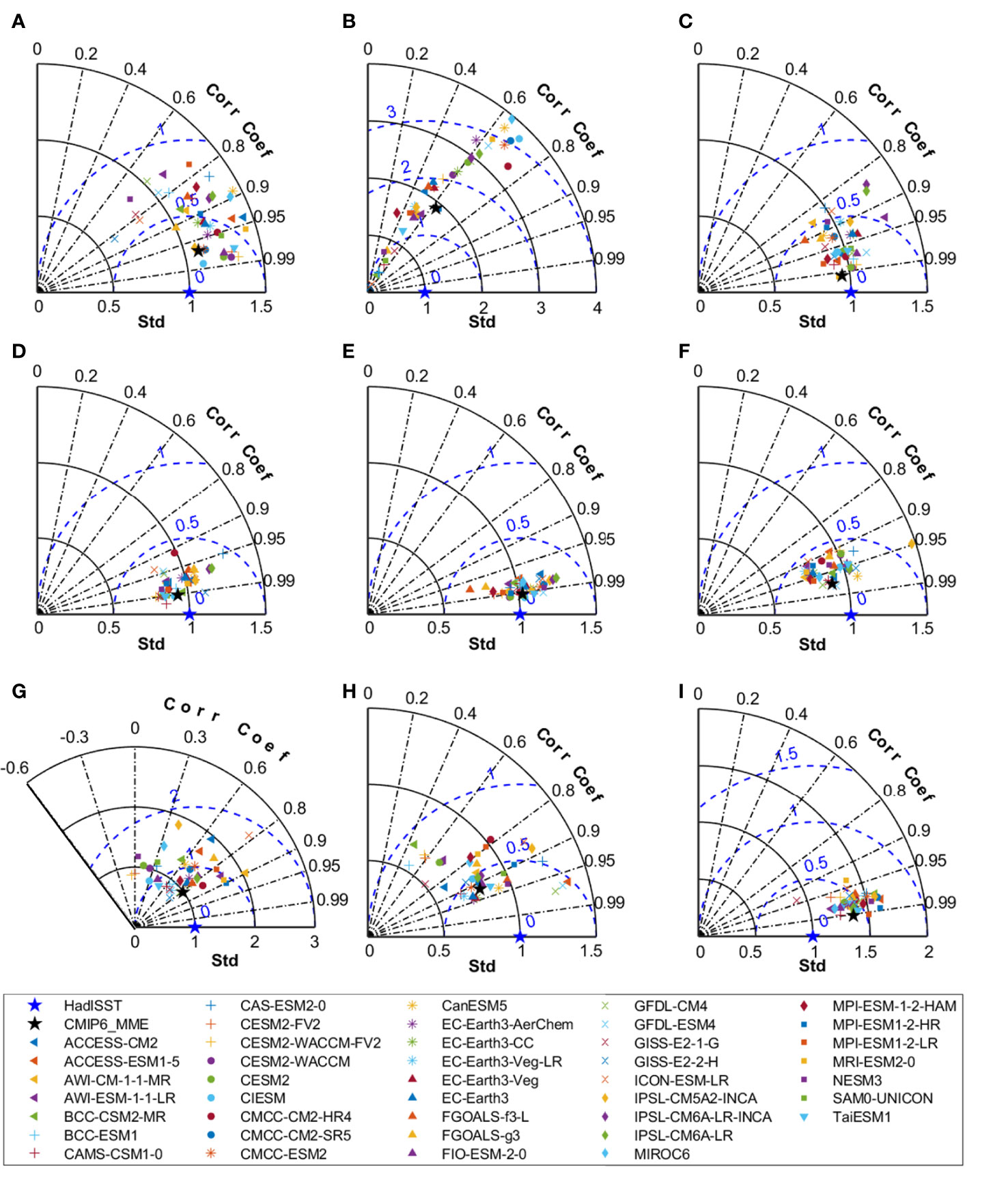
Figure 3 Taylor Diagram of simulated sea surface temperature in different regions of the Asian Marginal Seas (AMS) in boreal winter in the CMIP6 models. (A) Bering Sea; (B) Sea of Okhotsk; (C) Japan/East Sea (JES); (D) East China Seas (ECSs); (E) Philippine Sea; (F) South China Sea (SCS); (G) Indonesian seas; (H) Bay of Bengal; (I) Arabian Sea. The black solid circles indicate the normalized spatial standard deviation (σ_M/σ_O) with respect to that of HadISST (σ_O). The dashed blue contours and dashed black lines indicate the centered root-mean-square bias (E′) and spatial correlation coefficient (R) of boreal winter climatological SST between models and HadISST, respectively. The HadISST is defined as the reference point (blue pentagram), with normalized spatial standard deviation (σ_O/σ_O), E′, and R equal to 1, 0, and 1, respectively. The black pentagrams donate the CMIP6 multi-model ensemble means (MMEs). The σ_M, σ_O, E′ and R are defined in Section 2.2.

Similar to Figure 3, the Taylor diagrams of AMS climatological SST in boreal summer are shown in Figure 4. In boreal summer, the “worst” simulation occurs in the South China Sea and the Bay of Bengal, as revealed by their smallest correlation (−0.3< R< 0.8 in the SCS and −0.5< R< 0.78 in the Bay of Bengal), widely spread spatial standard deviation (1< σ< 4 in most of the models), and largest centered RMS error (E’ > 1 and up to 6) (Figures 4F, H). In the South China Sea and the Bay of Bengal, the simulated climatological SSTs in 15% and 37% of the CMIP6 models are not significantly positively correlated with that of observation. The climatological SST is also not well reproduced in the Sea of Okhotsk, because less than half of the analyzed CMIP6 models show positive spatial correlation with the observed climatological SST above the 95% confidence level, albeit with a relatively small spatial standard deviation (0.3< σ< 1.4 in most models) and centered RMS error (E’< 1.75 in most models) (Figure 4B). The CMIP6 models show the “best” simulation of climatological SST in the Japan/East Sea, with R > 0.9, 0.7< σ< 1.35, and E’< 0.5 in most models (Figure 4C). There are also high spatial correlations (R > 0.9 for most of the models) in the East China Seas, but with a widely spread spatial standard deviation (0.5< σ< 3) and a centered RMS error (0.2< E’< 1.8) (Figure 4D). These results suggest that the climatological SST patterns in East China Seas are well reproduced in the CMIP6 models. However, large discrepancies exist among the CMIP6 models in terms of spatial differences and simulation biases. The simulated climatological SST generally shows positive correlations above the 95% confidence level with the observation in the Bering Sea (R >0.4), the Philippine Sea (R > 0.4), the Indonesian seas (R > 0.5), and the Arabian Sea (R > 0.6), suggesting reasonable climatological SST patterns simulated by most CMIP6 models in these regions (Figures 4A, E, G, I). In terms of the spatial deviation and the centered RMS error, they are generally in a range of 0.5< σ< 1.5 and E’< 0.75 in the Arabian Sea (Figure 4I), and range of 1< σ< 2 and E’< 1.5 in the Bering Sea, Philippine Sea, and Indonesian seas (Figures 4A, E, G).

FIGURE 4

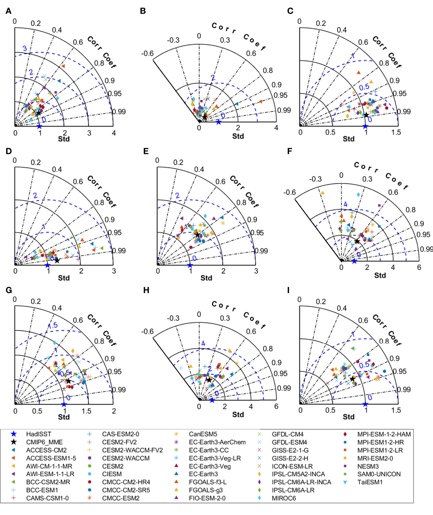
Figure 4 Same as Figure 3, but for boreal summer.

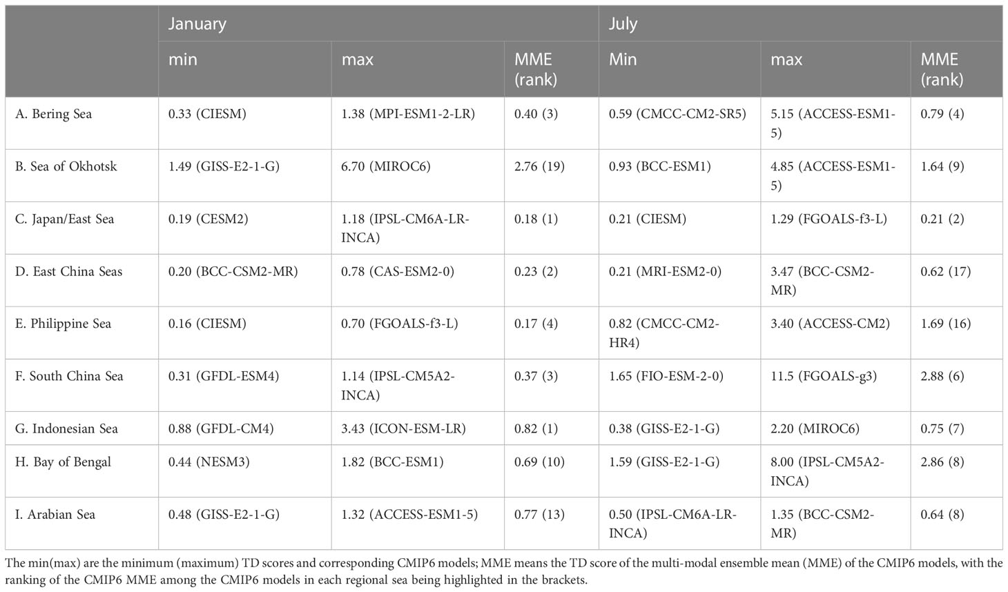
Table 2 gives the TD scores of the simulated climatological SST in the AMS regional seas in the CMIP6 models. In general, the simulated climatological SSTs of the MME are better represented in the Philippine Sea (TD Score = 0.17), Japan/East Sea (TD Score = 0.18), and East China Seas (TD Score = 0.23) in boreal winter, and in the Japan/East Sea (TD Score = 0.21), East China Seas (TD Score = 0.62), and Arabian Sea (TD Score = 0.64) in boreal summer. The Sea of Okhotsk (January) and the South China Sea (July) are the “worst” simulated regions, with TD scores of the MME climatological SST of 2.76 and 2.86, respectively. The CIESM gets the smallest TD scores in the Bering Sea (0.33) and Philippine Sea (0.16) in January, and in the Japan/East Sea (0.21) in July. The GISS-E2-1-G gets the smallest TD scores in the Sea of Okhotsk (1.49) and Arabian Sea (0.48) in January, and in the Indonesian seas (0.38) and the Bay of Bengal (1.59) in July. Meanwhile, the CESM2, BCC-CSM2-MR, GFDL-ESM4, GFDL-CM4, and NESM3 get the smallest TD scores in the Japan/East Sea, East China Seas, South China Sea, Indonesian seas, and Bay of Bengal in January, respectively; and the CMCC-CM2-SR5, BCC-ESM1, MRI-ESM2-0, CMCC-CM2-HR4, FIO-ESM-2-0, and IPSL-CM6A-LR-INCA get the smallest TD scores in the Bering Sea, Sea of Okhotsk, East China Seas, Philippine Sea, South China Sea, Arabian Sea in July, respectively. It is worth mentioning that the MME climatological SSTs could depress the cross-model biases in the Bering Sea and Japan/East Sea in both boreal winter and summer, as evidenced by the MME climatological SSTs therein obtain relatively higher ranks among the CMIP6 models.

TABLE 2

Table 2 Details of TD Score.

Figure 5 shows the TD values of the AMS climatological SST in boreal winter and summer, with smaller values implying better simulation skill. The CMIP6 MMEs get better results than most of the CMIP6 models by averaging the errors and biases in both boreal winter and summer, with scores of 0.1 and 0.2, ranking fifth and second, respectively. In boreal winter, the FIO-ESM-2-0 model gets TD scores of 0.08, ranking in the first place, followed by the CIESM, GFDL-CM4, and IPSL-CM6A-LR-INCA models, which get TD scores of 0.09. The climatological SST patterns in Asian marginal seas are better reproduced in these models than those in the CMIP6 MME. In boreal summer, the MPI-ESM-1-2-HAM has a better climatological SST simulation than the CMIP6 MME, with a TD score of 0.11, ranking in the first place. The boreal summer climatological SSTs are also well simulated in EC-Earth3, EC-Earth3-Veg, and EC-Earth3-Veg-LR, with TD scores smaller than 0.13, whereas the TD scores of these models exceed 0.13 in boreal winter. The GISS-E2-1-G ranks at the end both in boreal winter and summer, with TD scores of 0.3 and 0.63, respectively. There are only 5 models that have produced better climatological SST simulations in boreal summer than in boreal winter, e.g., CAS-ESM2-0, EC-Earth3, EC-Earth3-Veg, EC-Earth3-Veg-LR, and MRI-ESM-1-2-HAM. According to climatological SST simulation results, the models with large difference between the boreal winter and summer are IPSL-CM6A-LR-INCA and CAS-ESM2-0. The IPSL-CM6A-LR-INCA has better simulated climatological SST in boreal winter than summer, with TD scores of 0.09 and 0.43, ranking 4^th and 37^th in boreal winter and summer, respectively. Whereas, the CAS-ESM2-0 has better simulated climatological SST in boreal summer than winter, with TD scores of 0.17 and 0.23, ranking 10^th and 39^th in boreal summer and winter, respectively.

FIGURE 5

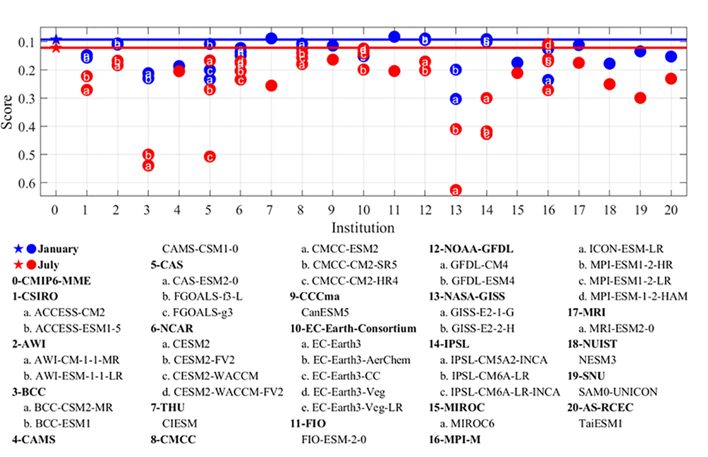
Figure 5 Taylor Diagram Score of the simulated climatological sea surface temperature (SST) in the Asia Marginal Seas (AMS). Blue and red pentagrams indicate the CMIP6 multi-model ensemble means (MMEs) in boreal winter and summer, with scores of 0.1 and 0.12, respectively. The sequence numbers from 1 to 20 are affiliated to the institutions as listed in Table 1.

4 Projected warming trend under different emission scenarios

According to HadISST observation, the SST shows the largest warming trend in the East China Seas and the Japan/East Sea since the Industrial Revolution (1871 – 2014), with values up to 1.5 and 1.2°C/century in boreal winter and summer, respectively (Figures 6A, B). Note that the maximum SST trend (~2.5°C/century) occurs near the Bering Strait in boreal summer. In the AMS, the warming trends in the Bering Sea and Sea of Okhotsk in January are the smallest, with values of approximately 0.05 and −0.2°C/century. In the AMS tropical regions, the warming trends are in a range of 0.2 – 0.8°C/century, roughly equal to half of those in the East China Seas and the Japan/East Sea. In July, the warming trends are greater than those in January in the AMS except for the East China Seas and the Japan/East Sea, with values of 0.4 – 1.2°C/century in the Bering Sea and Sea of Okhotsk, and 0.3 – 0.7°C/century in the AMS tropical regions. It should be noted that the boreal summer SST tends to get warm faster in the eastern Sea of Okhotsk than in the west.

FIGURE 6

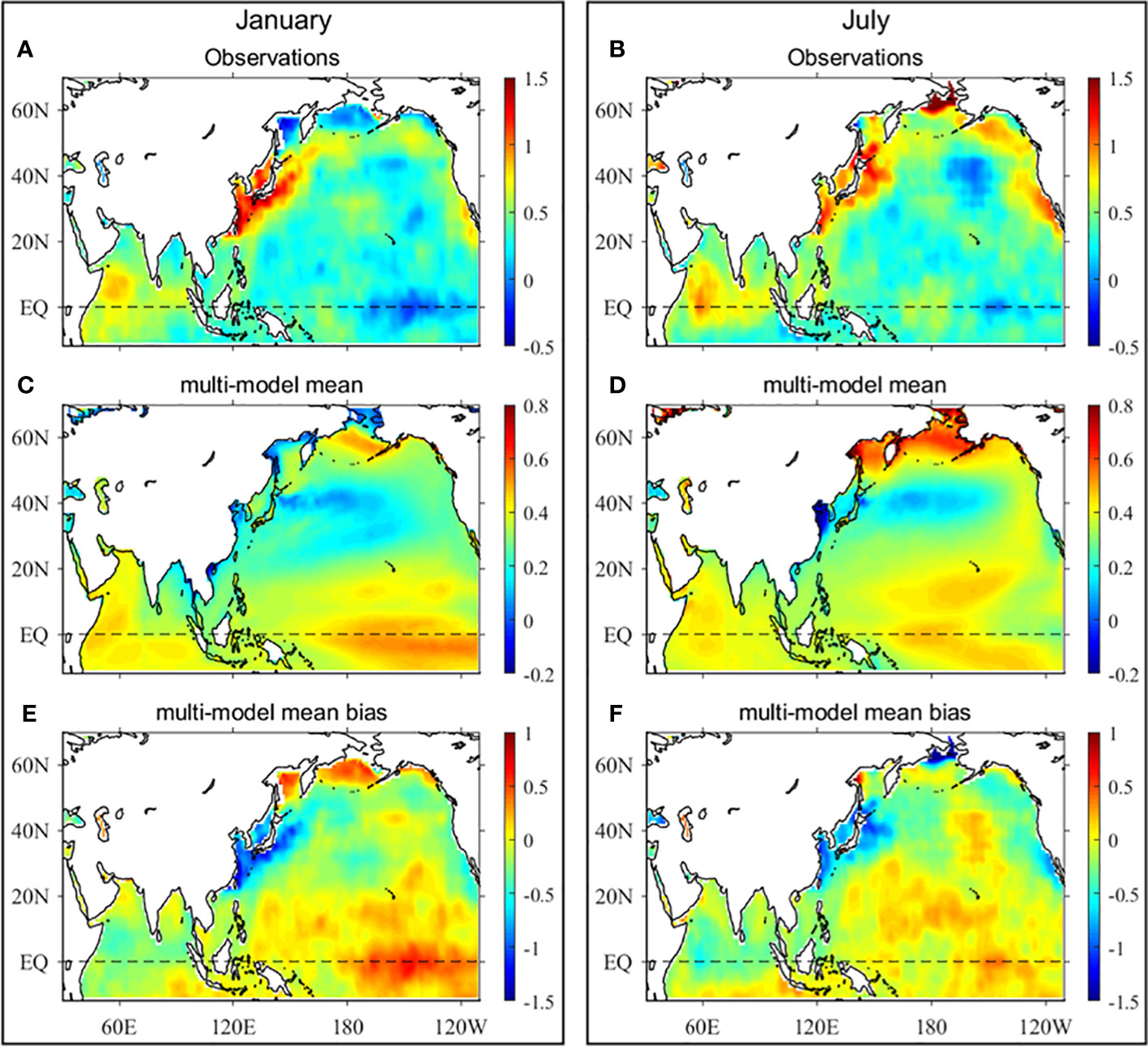
Figure 6 Linear trend in the sea surface temperature (SST) since the Industrial Revolution (Unit: °C/century). (A) January, and (B) July in HadISST observation (1871 – 2014); (C) January, and (D) July in the multi-model ensemble means (MME) of the CMIP6 historical simulation (1871 – 2014); and biases between the CMIP6 MME and HadISST in (E) January, and (F) July.

However, the simulated SST trend shows the largest value in the Bering Sea (0.5°C/century), whereas the smallest values are found in the west coast of the Sea of Okhotsk (0.1°C/century), the East China Seas (0.1°C/century), and the northern South China Sea (−0.05°C/century) in January (Figure 6C). The simulated SST trend shows the largest values in the Bering Sea (0.6°C/century) and the Sea of Okhotsk (0.7°C/century), whereas the smallest values are found in the East China Seas (−0.05°C/century) in July (Figure 6D). These distributions are in contrast to the observations. The simulated SST trends are generally smaller than observations in the Philippine Sea, Indonesian seas, Bay of Bengal, and Arabian Sea in both the boreal winter and summer, with values of approximately 0.15 – 0.45°C/century in the CMIP6 models and 0.3 – 0.7°C/century in the observations (Figures 6C, D). The differences between the simulated and observed SST trends in January and July are shown in Figures 6E, F. For the simulation of SST trend, the area below the significance level is found in the East/Japan Sea, East China Seas, and the Kuroshio basin. The warming trends in the East China Seas and the Japan/East Sea are underestimated by approximately 0.6 – 1°C/century in both January and July, and by 1.5°C/century in the Bering Strait in July. On the contrary, the warming trends are overestimated by up to 0.5°C/century in the Bering Sea and Sea of Okhotsk in January and approximately 0.1 – 0.4°C/century in the western Sea of Okhotsk and northwestern Bering Sea in July. In the AMS tropical regions, there are either over- or under-estimated SST trends with relatively smaller biases, roughly in a range of −0.2 to 0.05°C/century. The negative SST trend in the tropical Pacific and the positive trend in the northwest Pacific in the historical simulation seem to be connected to the unrealistic representation of the Interdecadal Pacific Oscillation in the models (England et al., 2014).

In addition to the SST trend in the AMS from the past to the present, it is also important to know how the SST will change in the future. Figure 7 illustrates the spatial pattern of AMS SST changes in the future period (2015 – 2100) under the SSP126, SSP245 and SSP585 scenarios. It should be noted that the color scales in the top, middle, and bottom panels are not identical. The SST trend distribution of the CMIP6 multi-model mean shows similar features under different future scenarios, with larger warming trends in the high latitudes whereas smaller warming trends in the mid- and low- latitude. The boreal winter SST warming trends are generally smaller than those of summer SST in the middle and high latitudes of the AMS (Figure 7). Meanwhile, the AMS SST warming trends increase from the equator to the high latitudes in both January and July under the SSP126, SSP245, and SSP585 simulations, indicating a more sensitive response of high latitude seas to global warming. In January, the larger SST warming trends occur in the Bering Sea and Sea of Okhotsk, with values up to 1.8°C/century in the SSP126 scenario (Figure 6A). In the SSP245 and SSP585 scenario, the larger SST warming trend occurs in east coast of the Bering Sea, exceeds 3.5 and 6.5°C/century in January, respectively (Figures 6C, E). In July, the larger SST trends occur in the Bering Sea, Sea of Okhotsk, the northern Japan/East Sea, and the Bohai Sea, with values up to 2.7, 5, and 9°C/century in the SSP126, SSP245 and SSP585, respectively.

FIGURE 7

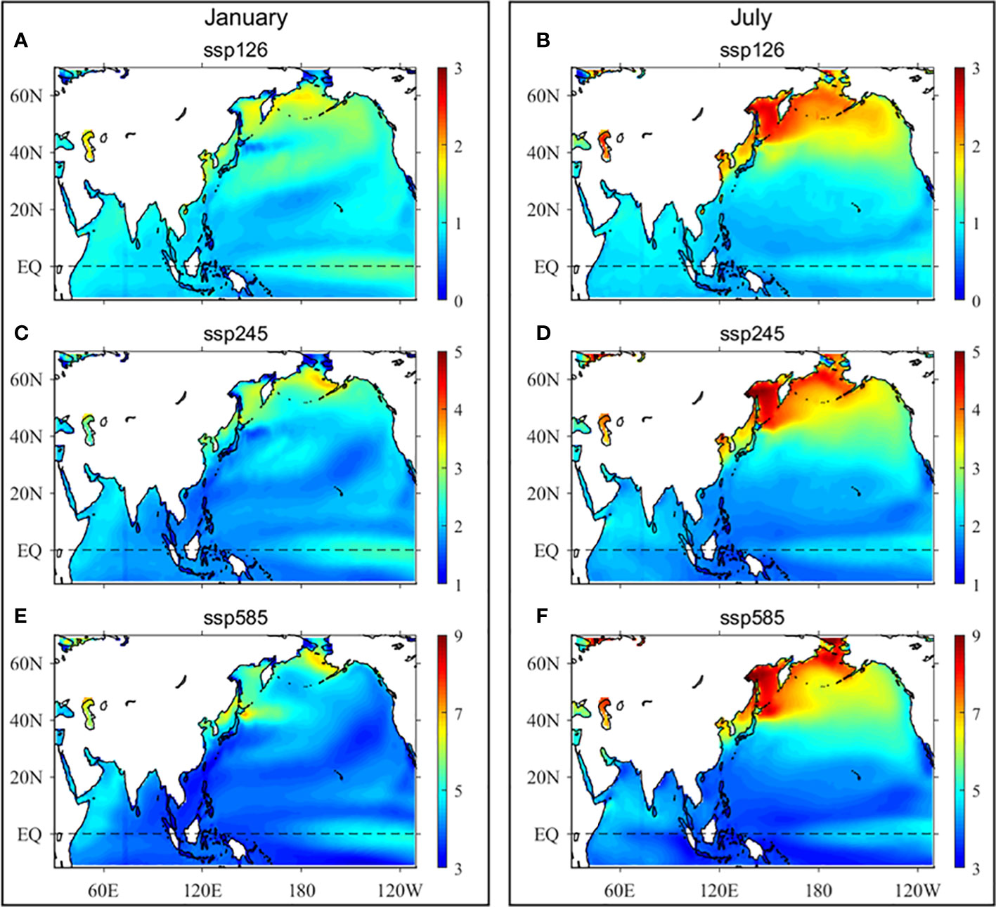
Figure 7 Linear trend in the sea surface temperature (SST) for the future scenario simulations under Shared Socio-Economic Pathway (SSP) in CMIP6 models (Unit: °C/century) (2015–2100). (A) January, and (B) July in SSP126; (C) January, and (D) July in SSP245; and (E) January, and (F) July in SSP585.

Figures 8 and 9 show the time series of regional average SST changes from observation and CMIP6 models in January and July, respectively. In January, the SST trends between the observation and simulation show larger biases in the high-latitudes (e.g., the Bering Sea, Sea of Okhotsk, JES, and ECSs), whereas smaller biases are found in the tropical marginal seas (e.g., the Philippine Sea, SCS, Indonesian seas, Bay of Bengal, and Arabian Sea) (Figure 8). In January, the SST trend is overestimated in CMIP6 models in the Bering Sea, with more than three times the observation (Figure 8A). In the Sea of Okhotsk, the SST warming is not obvious in observation, but obvious in the simulation result, with a warming trend of 0.28°C/century in January (Figure 8B). The SST trends simulated by the CMIP6 models are underestimated in the JES and ECSs, with less than one-third of the observation in January (Figures 8C, D). In July, the SST trends between the observation and simulation show larger biases in the JES and ECSs, whereas smaller biases in other AMS (Figure 9). For the AMS, the largest SST trends are found in the JES and ECSs in observation (~ 0.9°C/century), whereas 0.32 and 0.12°C/century in CMIP6 models, respectively (Figures 9C, D).

FIGURE 8

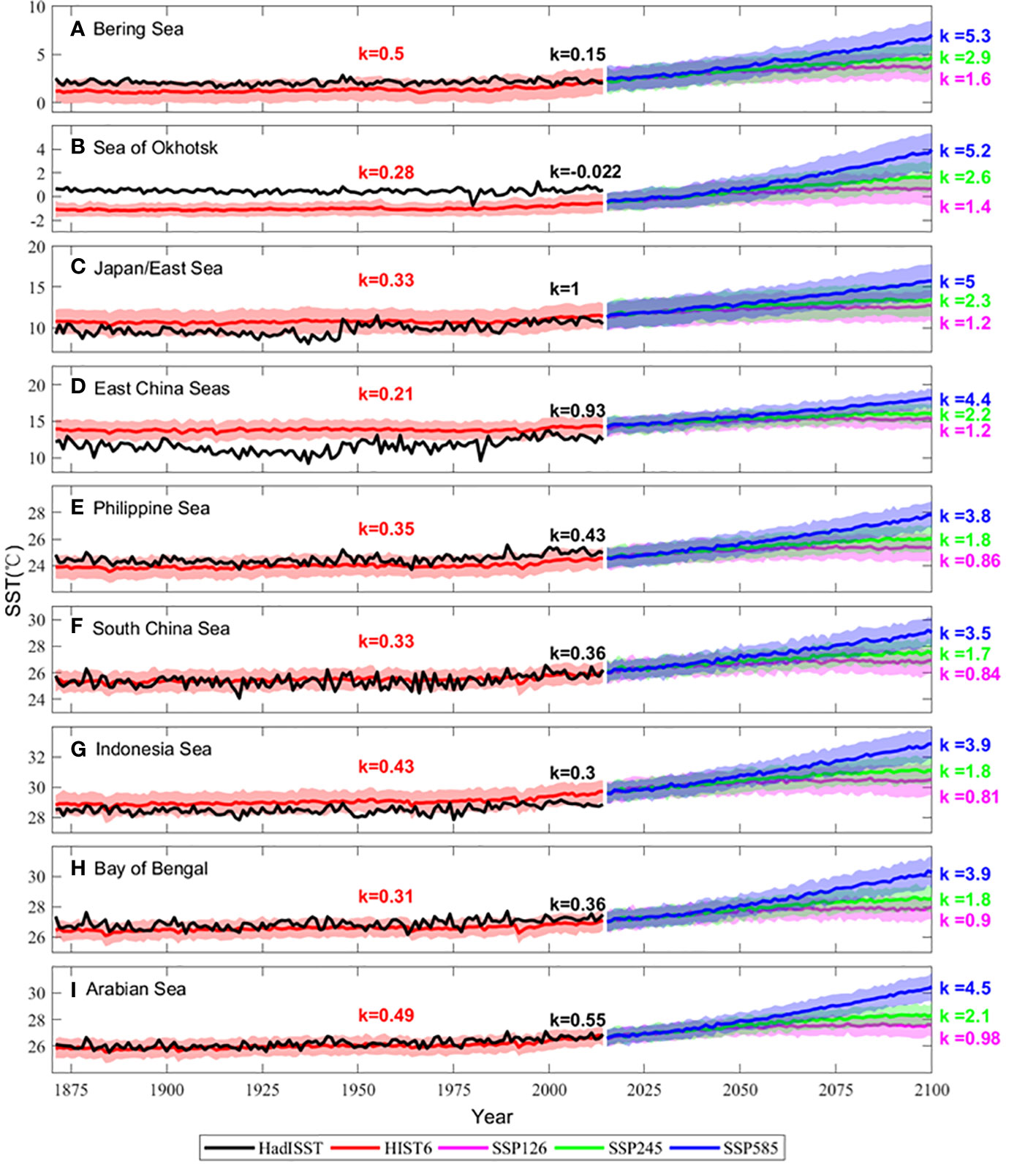
Figure 8 Time series of regional average Sea Surface Temperature (SST; unit: °C) from observation (black), multi-model ensemble means (MME) of the CMIP6 historical simulation (red), MME of the simulations under SSP126 (pink), SSP245 (green) and SSP585 (blue) with the uncertainty between the models (shaded) for the Asian Marginal Seas (AMS) in January. (A) Bering Sea; (B) Sea of Okhotsk; (C) Japan/ East Sea (JES); (D) East China Seas (ECSs); (E) Philippine Sea; (F) South China Sea (SCS); (G) Indonesian seas; (H) Bay of Bengal; (I) Arabian Sea). The ‘k’ means the SST trend for historical (1870 – 2014) or future (2015 – 2100) period (unit: °C/century), the different color of ‘k’ corresponds to the colorful line.

FIGURE 9

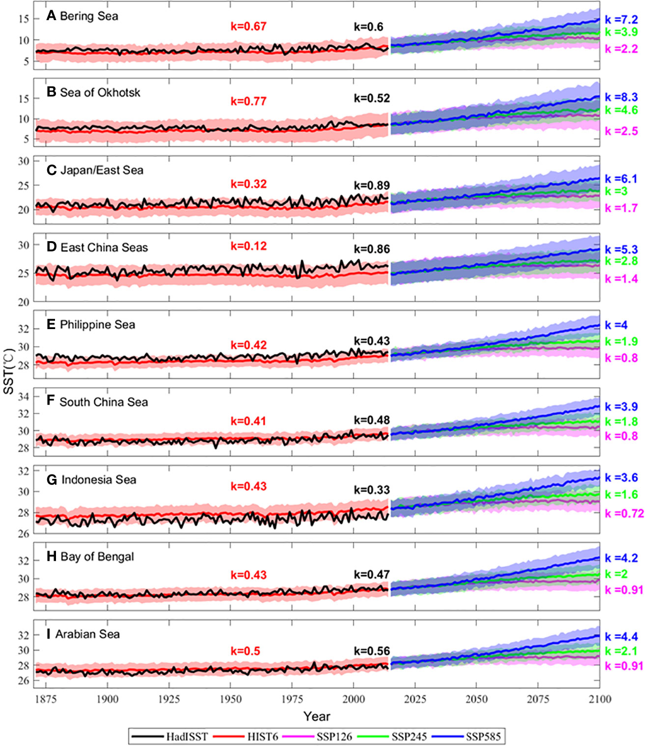
Figure 9 Same as Figure 8, but in July.

In the historical period (1870 – 2014), the interannual changes of SST simulated by the CMIP6 models are not obvious compared with the observation. From the historical simulation results of CMIP6 models, it can be found that the SST trends have been significantly enhanced since 1990. In the JES and ECSs, the spatial mean SST trends for the present-day period (1990 – 2014) are 2.7 – 4.7°C/century, more than 40 times the past-day (1870 – 1990) value which is less than 0.1°C/century in the CMIP6 models. In the other AMS, the spatial mean SST trend for the present-day period (1990 – 2014) is approximately 10 times the past-day (1870 – 1990) value of ~ 2.5°C/century (in January) and approximately of 3°C/century (in July) in the CMIP6 models. Significantly enhanced SST trend since 1990 has not appeared in the observation. In the future period (2015 – 2100), the CMIP6 models have similar SST trends until 2030 under different future scenarios in the marginal seas. Under SSP126 and SSP245, the SST warming trend in the early 21st century will be significantly stronger than that of the late 21st century. But under SSP585, the SST warming trend in the later 21st century will be significantly stronger than that of the early 21st century. Same characteristics are also found in the analysis of the SCS based on the CMIP5 models (Huang et al., 2014).

The SST trends of the global annual mean for HadISST, historical, SSP126, SSP245 and SSP585 are 0.38, 0.3, 0.8, 1.74, and 3.77°C/century, respectively (Figure 10A). In the AMS, the most significant observed SST trends of the annual mean are found in the JES and ECSs, with the SST trends being about 2.6 times the global mean, which is the same as that concluded by Sasaki and Umeda (2021) (Figure 10A). The observed SST trends of the global mean are 0.24 and 0.55°C/century in January and July, respectively (Figures 10B, C). In the JES and ECSs, the observed SST warming trends exceed four times the global mean in January and about 1.6 times in July (Figures 10B, C). In the CMIP6 historical simulation, the smallest simulated SST trends are found in the JES and ECSs, both in their annual means, January, and July, smaller than the global mean (Figure 10). In the other Asian Marginal Seas, the historical simulated SST warming trend is similar to the global mean. In the CMIP6 future scenarios, stronger SST warming trends are found in the high latitudes (e.g., the Bering Sea, Sea of Okhotsk, JES, and ECSs) and are approximately 1.5 – 2 times higher than the global mean (Figure 10). The larger the emissions (SSP585 > SSP245 > SSP126), the larger difference in the SST trends between the global mean and the AMS. The difference in SST trends between high- and low-latitudes is more significant in July than in January (Figures 10B, C).

FIGURE 10

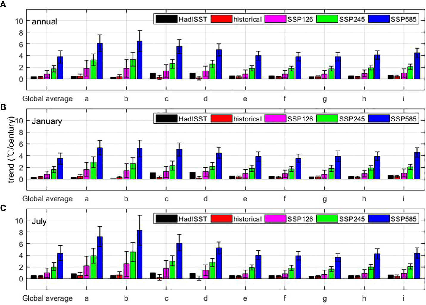
Figure 10 Trends of spatial mean SST in the global and each Asian Marginal Sea (unit: °C/century). (A) annual; (B) January; (C) July. (a. Bering Sea; b. Sea of Okhotsk; c. Japan/East Sea (JES); d. East China Seas (ECSs); e. Philippine Sea; f. South China Sea (SCS); g. Indonesian seas; h. Bay of Bengal; i. Arabian Sea).

5 Discussion

In this study, larger SST bias and inter-model diversity are found in the East/Japan Sea and the East China Seas. In the previous studies, it has been pointed out that the dynamical processes causing intermodel diversity in simulating East AMS SST during the near-future period (2020 – 2049) may be not limited to local variables, but linked to Pacific Ocean basin-scale processes, and the inter-model diversity in simulating East AMS SST is influenced by both atmospheric and oceanic processes associated with the North Equatorial Current bifurcation latitude (Yi and Yeh, 2019). These findings suggest that in order to reduce AMS SST uncertainties from CMIP6 climate models, it is critical to correctly simulate the tropical Pacific mean state simulations. In addition, there also exists a large difference between the observations (HadISST, EN4, COBE, ERSST, and OIsst) in the East/Japan Sea and the East China Seas (see Figures A1-A3 in the appendix).

Based on the large SST historical simulation biases in some of the AMS, the credibility of the future estimates is questioned. Here, we discuss the relationship between historical simulations and future predictions in terms of both spatial pattern and trend. Figure 11 gives the correlation coefficients of the climatological SST spatial pattern between the model historical simulation and future projection and we find that all correlation coefficients are larger than 0.7 and above the 95% confidence level. In the spatial pattern of SST, the correlation between historical simulation and future projection is more significant. For the correlation between inter-model similarities in spatial pattern for present and projected future mean climate (Abe et al., 2009), the correlation is only small for historical simulation and SSP126 in January (see Figures A4-A5 in the appendix).

FIGURE 11

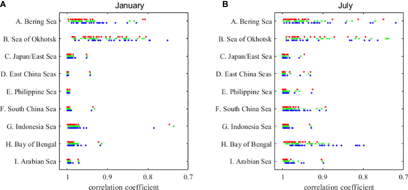
Figure 11 Correlation coefficients of the climatological SST spatial pattern between the model historical simulation and future projection in (A) January and (B) July. The red, green, and blue dots indicate the correlation coefficients between historical simulation and SSP126, SSP245, and SSP585 projection, respectively.

Figure 12 gives the causation analysis of SST between historical simulation and future projection based on Liang (2014), with the area marked by dots indicating that it is above the 90% significance level. The causation between historical simulation and future projection is calculated by the SST time series on each longitude-latitude point. It is found that the SST of historical simulation isn’t the cause of the future projection in most AMS regions. In other words, the historical simulated SST affects the SST predictions in the Japan/East Sea and northwestern Bay of Bengal under the SSP126, in the central Bay of Bengal under the SSP245, and in the southern Arabian Sea under the SSP585 (the area marked by dots). Therefore, in regions other than the above-mentioned seas, we can assume that the historical simulation trend biases have less impact on the future projection.

FIGURE 12

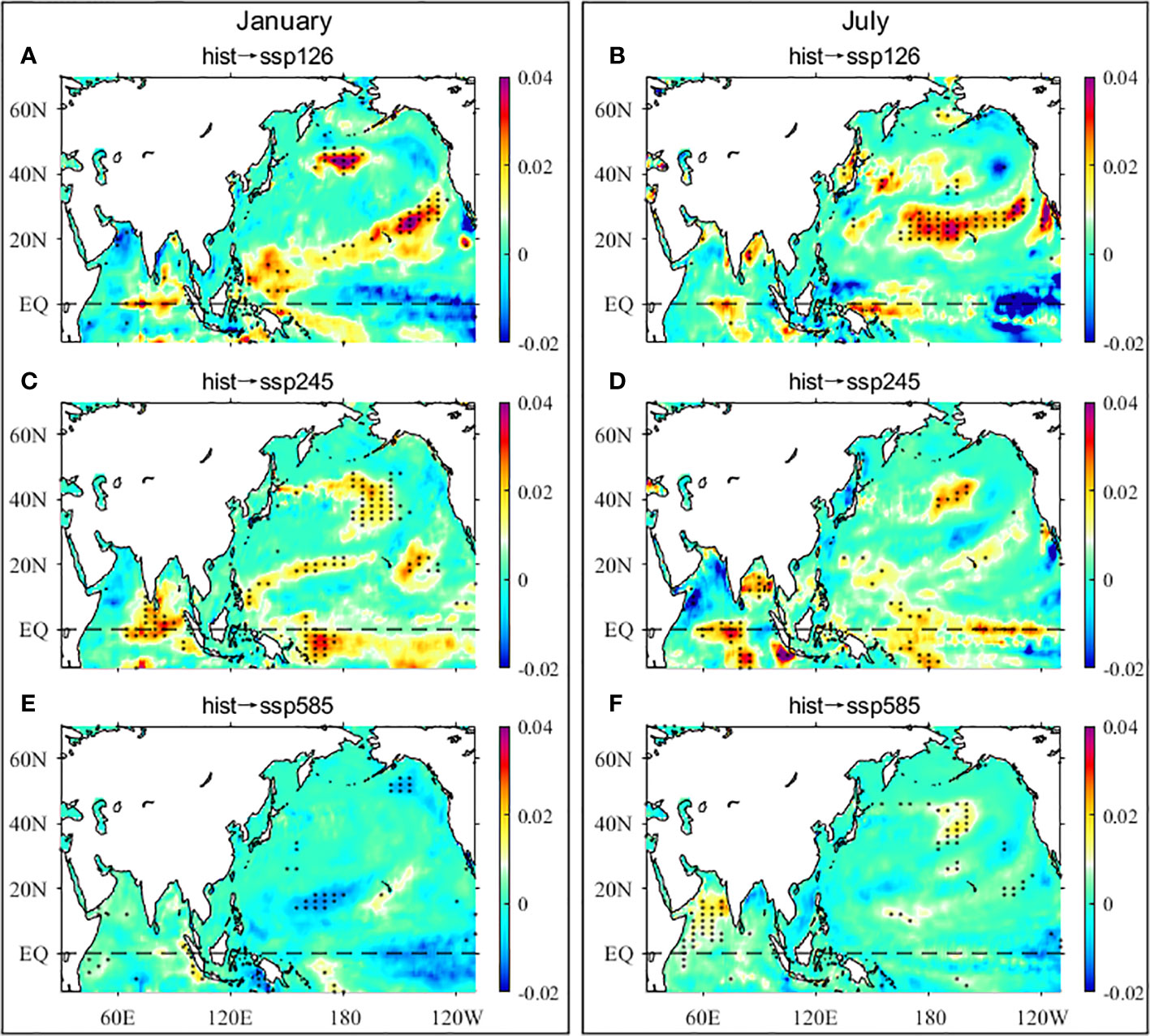
Figure 12 Information flow of SST between historical simulation to future projection in January (left column) and July (right column) (unit: nats/year). (A, B) hist→ssp126; (C, D) hist→ssp245; (E, F) hist→ssp585. The area marked by dots indicating that above the 90% significance level.

6 Conclusions

The representation of the simulation of CMIP6 models for the Asian Marginal Seas has been evaluated in this paper. The AMS climatological SST simulated by the CMIP6 multi-model ensemble mean (MME) basically shows similar patterns to observations in boreal winter and summer, as well as the amplitudes of seasonal variations. In boreal winter, the largest positive biases occur in the JES and the ECSs (up to 2°C), while the largest negative biases occur in the Sea of Okhotsk (up to −2°C). In boreal summer, the largest positive biases occur in the Indonesian seas and along the west coast of Africa in the Arabian Sea (approximately of 1.2−1.5°C) and the largest negative biases occur in the Sea of Okhotsk, the Bohai Sea, and the northern ECS (exceeding −2°C). In the JES and ECSs, the amplitudes of seasonal variations are significantly underestimated due to warmer SST in boreal winter and colder SST in boreal summer.

From the Taylor Diagrams, the CMIP6 models show the “best” simulation of climatological SST in the Philippine Sea and the “worst” simulation in the Sea of Okhotsk in boreal winter. In boreal summer, the “best” climatological SST simulation of the CMIP6 models is found in the JES, and the “worst” simulation is found in the South China Sea and the Bay of Bengal. Additionally, the climatological SST simulations using the multi-model ensemble mean of CMIP6 models are better than those obtained using single model, both in the spatial distribution and the values of SST. For simulations of the entire AMS, the CMIP6 MMEs get better results than most CMIP6 models by averaging the errors and biases in both boreal winter and summer, with scores of 0.1 and 0.2, ranking fifth and second, respectively. In CMIP6 models, the FIO-ESM-2-0 and the MPI-ESM-1-2-HAM have the best climatological SST simulations in boreal winter and summer, respectively. On the other hand, the GISS-E2-1-G has the worst climatological SST simulation both in boreal winter and summer.

According to HadISST observations, the SST shows the largest warming trend in the ECSs and the JES since the Industrial Revolution (1871–2014), both in boreal winter and summer. In the ECSs and the JES, the observed SST trends of the annual mean are about 2.6 times the global mean, which is the same as that indicated by Sasaki and Umeda (2021). In addition, the observed SST warming trends in theECSs and the JES exceed four times the global mean in January and are about 1.6 times the global mean in July. Note that the maximum SST trend occurs near the Bering Strait in boreal summer. However, the simulated SST trends are generally smaller in the East China Seas and the Japan/East Sea, with values less than one-third of the observation in January. In January, the simulated SST trends show larger biases in the high latitudes, with more than three times the observation, whereas smaller biases are shown in the tropical marginal seas. In July, the larger SST trends biases between the observation and simulation are found in the JES and ECSs, whereas smaller biases are found in other AMS. In addition, the simulated SST trends have been significantly enhanced since 1990 in the CMIP6 historical simulation. In the JES and ECSs, the spatial mean SST trend for the present-day period (1990 – 2014) is more than 40 times greater than the past-day (1870 – 1990) trend in the CMIP6 models.

In the future period (2015 – 2100), the SST trend distributions of the CMIP6 multi-model mean show similar features under different future scenarios, with larger warming trends in the high latitudes and smaller trends in the mid- and low-latitudes. In the high- and mid-latitudes, the SST trends are generally smaller in boreal winter than those in summer. Meanwhile, the AMS SST warming trends increase from the equator to the high latitudes in both January and July under the SSP126, SSP245, and SSP585 simulations, indicating a more sensitive response of the high latitudes to global warming. In addition, the CMIP6 models have similar SST trends until 2030 under different future scenarios in the marginal seas. Under SSP126 and SSP245, the SST warming trend in the early 21st century will be significantly stronger than that of the late 21st century, whereas the opposite is true for SSP585.

The rapid warming of the SST can affect the habitat range of fish. In temperate coastal waters of Japan, the habitat range of harmful fish is estimated to increase to 1.2 – 1.9 times that of 2000 – 2018 with severe warming, whereas it will not change significantly with stringent mitigation by the 2090s (Sudo et al., 2022). The SST warming can also influence marine pelagic biodiversity, though with a minor influence under the SSP126. Worryingly, the severe warming will affect marine pelagic biodiversity to a greater extent than temperature changes that took place between either the Last Glacial Maximum or the mid-Pliocene and today (Beaugrand et al., 2015). In order to maintain stable ecological environment and avoid or reduce extreme weather, it is necessary to limit the SST trend to a certain range, which provides a theoretical basis for the government to formulate emission plans. In addition, a warming sea surface background would also benefit to enhanced intensity and increased frequency of marine heatwaves, which would not only have a devastating impact on the marine habitats of the AMS but also threaten our society by inducing land heatwaves. Such effects have already been observed by high resolution satellite-based SST in the JES in terms of marine heatwaves (Wang et al., 2022; Chen et al., 2023) and the occurrence of coral bleaching in the JES (Hwang et al., 2017).

Data availability statement

Publicly available datasets were analyzed in this study. This data can be found here: The observed SST data is available at https://climatedataguide.ucar.edu/climate-data/sst-data-hadisst-v11. The SST data from CMIP6 models is available at https://esgf-node.llnl.gov/projects/cmip6/.

Author contributions

TX, SJ and ZW conceptualized the research. SJ executed the research and drafted the manuscript. DW processed the CMIP6 data. All authors contributed to the article and approved the submitted version.

Funding

This study is jointly supported by the Laoshan Laboratory (No. LSKJ202202700), the National Natural Science Foundation of China (NSFC) Projects (42076024, 42076023, 41821004), and the Global Change and Air-Sea Interaction II (Contact No.GASI-01-ATP-STwin).

Acknowledgments

We thank Haidong Pan for linguistic assistance and pre-submission expert review.

Conflict of interest

The authors declare that the research was conducted in the absence of any commercial or financial relationships that could be construed as a potential conflict of interest.

Publisher’s note

All claims expressed in this article are solely those of the authors and do not necessarily represent those of their affiliated organizations, or those of the publisher, the editors and the reviewers. Any product that may be evaluated in this article, or claim that may be made by its manufacturer, is not guaranteed or endorsed by the publisher.

Supplementary material

The Supplementary Material for this article can be found online at: https://www.frontiersin.org/articles/10.3389/fmars.2023.1178974/full#supplementary-material

References

Abe M., Shiogamo H., Hargreaves J. C., Annan J. D., Nozawa T., Emori S. (2009). Correlation between inter-model similarities in spatial pattern for present and projected future mean climate. SOLA. 5, 133–136. doi: 10.2151/sola.2009-034