Forecast uncertainty and ensemble spread in surface currents from a regional ocean model

An operational ocean Ensemble Prediction System (EPS) for the coastal seas off Northern Norway is evaluated by comparing with high-frequency radar current speed estimates. The EPS is composed of 24 members for which the ocean current is not perturbed nor constrained but forced with an atmosphere ensemble. The ocean ensemble spread stems from (i) accumulated differences in wind-forcing history and (ii) constraints of sea surface temperature by data assimilation. The intention of the ensemble is to reflect the actual uncertainty in initial conditions, which are largely unknown in terms of mesoscale circulation. We find a low but pronounced predictive skill in surface currents along with a good statistic skill. Additionally, current speeds show deterioration of the validation metrics over the forecast range. Further, high-resolution wind forcing seems to provide better forecast skill in currents compared to lower resolution forcing. In general, the ensemble exhibits the ability to predict forecast uncertainty.

1 Introduction

Surface currents are a pertinent ocean state variable for applications in marine ecosystems, offshore industries, and shipping. Forecasting of surface currents is particularly demanded in coastal seas, where considerable damage can be done by transported pollutants (e.g. Strand et al., 2020; Prasad et al., 2022). Risk assessments, ecosystem models, and impact studies require statistical descriptions of the current field, while emergency response situations require short-term forecasts (Christensen et al., 2018; Röhrs et al., 2023b).

Observation methods provide patchy coverage of surface currents with various representations of currents (e.g. Idžanović et al., 2017; Isern-Fontanet et al., 2017), while ocean general circulation models (OGCMs) can predict currents covering full spatial domains but suffering from intrinsic chaotic variability (Lorenz, 1969; Nonaka et al., 2016). Hence, a weakness in state-of-the-art OGCMs is that mesoscale current fields exhibit very limited predictability. Precise statistic skill in models satisfies some applications, whereas near-real-time decision making demands predictive model skill. Given deliberate model configuration, the statistic skill is generally achieved in operational models, but predictive skill requires constraints by observations (Jacobs et al., 2021). Ensemble Prediction Systems (EPS) are common means to predict model uncertainty, allowing to assess whether a forecast is reliable or not (Tilmann and Raftery, 2005; Pinardi et al., 2011; De Dominicis et al., 2016). EPSs can then be used to identify predictable features in ocean forecasts thereby adding value to forecast systems (Thoppil et al., 2021). Yet, it is necessary to show that the used ensemble reflects the uncertainty of the model in terms of verifying observations. Responding to a growing demand for high-resolution current forecasts in operational oceanography, we investigate the capability of a regional ocean EPS to quantify its uncertainty in current predictions.

Given appropriate accuracy in initial conditions and model resolution, deterministic forecasting of mesoscale circulation has been shown to be possible (Jacobs et al., 2014), but observations are often too sparse to encompass the full initial state. Certain degree of predictability may also prevail due to coastal constraints and dominant wind forcing (Kim et al., 2009; Cucco et al., 2016; Lima et al., 2019), e.g. during triggering of inertial waves and strong drift currents (Christensen et al., 2018). While only the flow features on constrained scales contain deterministic forecast skill, Jacobs et al. (2021) show that OGCMs may skillfully predict uncertainty on smaller scales if statistic skill is present at those scales.

Data assimilation techniques play a key role to provide initial conditions for models. While model resolution has been subsequently increased in recent years, observation networks have not followed to provide the same level of detail to constrain high-resolution circulation patterns. Hence, smaller scales in high-resolution ocean models are typically not constrained by observations. Models with high resolution have larger errors than their low-resolution counterparts (Sandery and Sakov, 2017). Spatial smoothing of surface currents reduces the error in drift forecasts, but in practice, removes variability in the non-constrained scales (Dagestad and Röhrs, 2019).

In this paper, we address surface currents of a regional OGCM, in which ocean currents are not actively constrained by assimilation of either satellite altimetry or high-frequency (HF) radar observations. Instead, HF radar radial currents are being used to assess the modeled current fields in terms of a single observed quantity. In addition, we assess the ensemble spread of an associated EPS and test the hypothesis that the EPS can quantify probabilities that certain radial current speeds are exceeded. The main question is to what extent do we expect predictability in radial currents from regional ocean models that do not assimilate currents or have few observations of currents.

Section 2 provides a description of data and methodologies used in this study. In section 2.1, we describe the validation data set and give an overview of the model set-up in section 2.2. The validation metrics for radial currents is presented in section 2.3. In section 3, we assess the modeled surface currents by looking into their flow patterns as well as the ensemble spread and its reliability. Finally, we discuss the results and give some concluding remarks on regional ocean modeling in section 4.

2 Data and methods

2.1 High-frequency radar data

Surface current retrieval from land-based HF radars was developed in the 1970s. The capacity of HF radars to measure currents at high spatial and temporal resolution over relatively large coastal areas make them a convenient system for operational purposes. Their signals are unaffected by rain, snow, wind, and other atmospheric events, but are affected by external interference (Isern-Fontanet et al., 2017). HF radars complement satellite altimetry observations which are limited to larger scales and suffer limitations when approaching the coast (Vignudelli et al., 2019), and represent an alternative to fill data gaps in data assimilation schemes (e.g. Gopalakrishnan and Blumberg, 2012).

HF radars exploit the Bragg resonance phenomenon to map ocean surface currents, wave fields, and increasingly winds in coastal areas (Hernandez-Lasheras et al., 2021). The basic mechanism of an HF radar system is the analysis of the backscattered radio wave to calculate surface currents. Emitted electromagnetic waves are backscattered by surface waves of exactly half the HF radar wavelength. Radial velocities (velocities towards or away from the antenna) are derived from the Doppler shift due to the difference between the theoretical and measured Bragg frequency (Barrick and Weber, 1977). E.g., at an operating frequency of around 13.25 MHz the measurement depth is approximately 0.9 m (Stewart and Joy, 1974). Accuracy of the radar-derived velocities has been shown to be typically in the range of 3-12 cm/s (Laws et al., 2011). Due to the complexity of the measurement principle, HF radar-based current data require careful interpretation. Nevertheless, HF radars have become one of the most important sources of surface current data in operational oceanography due to their ability to cover extended areas with high temporal resolution and to resolve a variety of ocean processes (e.g. Shay et al., 1995; Gough et al., 2010; Gurgel et al., 2011; Kirincich et al., 2013). Many studies in recent years focus on using HF radar-derived surface currents as sources for data assimilation (e.g. Oke et al., 2002; Barth et al., 2008), and in addition show good correlations for radial velocities and total vectors measured by HF radars and ADCPs (Cosoli et al., 2010).

In the present study, we use data from the CODAR SeaSonde instrument, operated by the Norwegian Meteorological Institute on the Fruholmen island (Figure 1) since October 2016 (B. Meldal-Johnsen, personal communication, 2022). The HF radar on Fruholmen emits at a central frequency of 4.453 MHz, reaching distances up to 180 km, with a range resolution of around 5 km. We used hourly radial velocities covering the period from mid-November to end of December 2021. Prior to conducting the analysis, some editing and quality assessment of the HF radar observations was performed. First, observations flagged as outside angular filter area were removed. In addition, spikes in the HF radar time series exceeding 0.75 m/s over an hour were removed (A. K. Sperrevik, personal communication, 2022). On average, around 2000 observation points per hour were available in the selected area. The HF radar data is available through THREDDS.

FIGURE 1

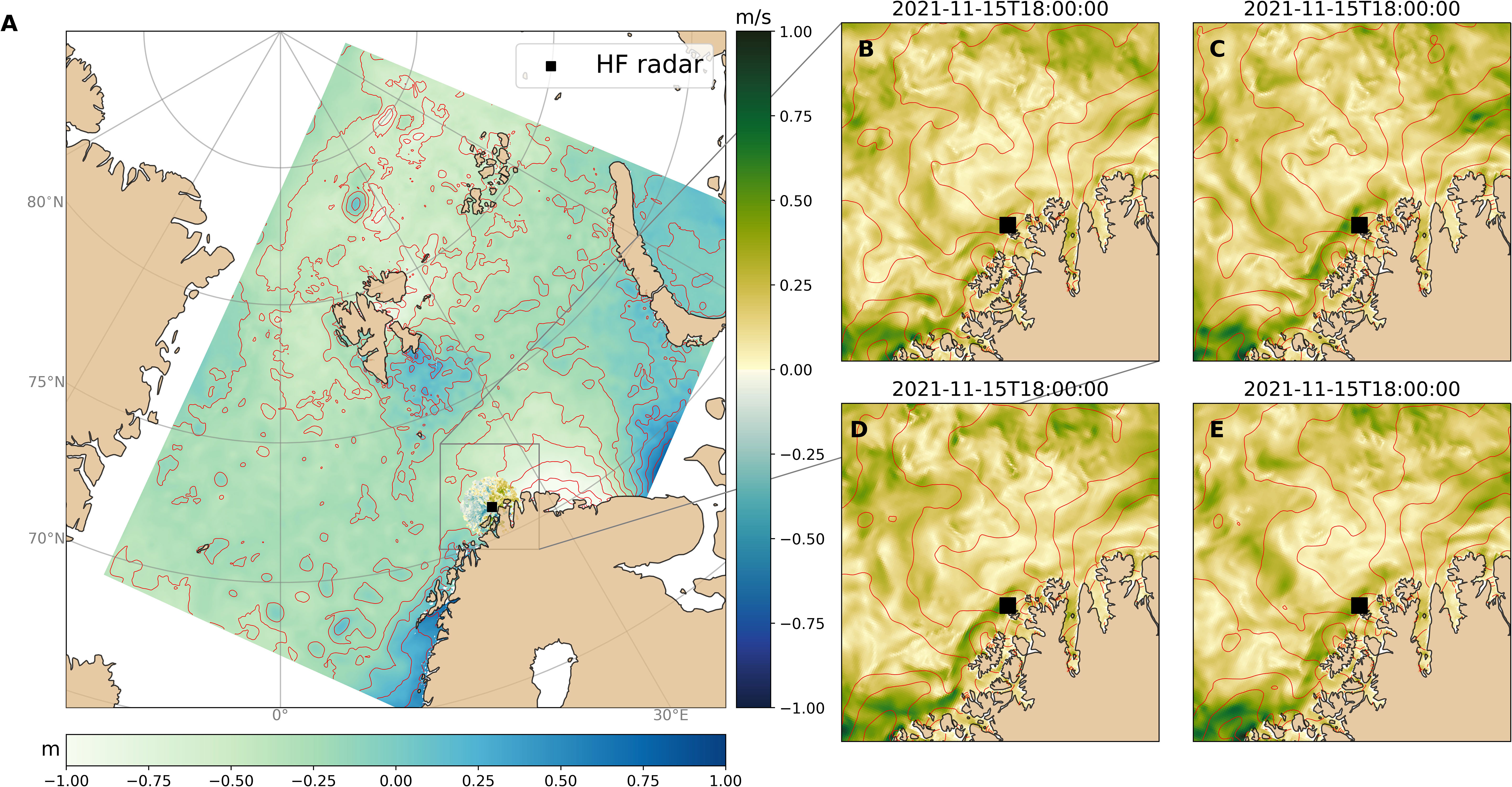
Figure 1 (A) Barents-2.5 EPS domain and location of the HF radar. Sea surface height (in m) with 0.2 m red contour lines from the model, as well as positive and negative radial velocities (in m/s) observed by the HF radar. (B–E) Surface current speed (yellow-green shading) and sea surface height (0.1 m red contours) from four random Barents-2.5 EPS members. All figures are snapshots on 2021-11-15 18:00.

2.2 Barents-2.5 Ensemble Prediction System

Barents-2.5 is a coupled ocean and sea-ice model covering the coast off Northern Norway, the Barents Sea, and Svalbard (Figure 1A). The model is implemented at the Norwegian Meteorological Institute and used as input for trajectory modeling during search-and-rescue operations and tracking of marine pollution. The model code is based on the METROMS framework (https://doi.org/10.5281/zenodo.5067164), which implements the coupling between the ocean component ROMS and the sea-ice component CICE (Fritzner et al., 2018; Fritzner et al., 2019). The Regional Ocean Modeling System (ROMS) solves the Reynolds averaged, hydrostatic primitive equations using a bottom-following coordinate system with free surface (Shchepetkin and McWilliams, 2005). Barents-2.5 has a horizontal resolution of 2.5 km with 42 stretched bottom following vertical layers, where the thickness of the uppermost layer varies between 0.5 m and 1 m. Turbulent mixing is parameterized using prognostic equations for turbulent kinetic energy and a generic length scale (Umlauf and Burchard, 2005). Further details on the model configuration and validation of sea-ice concentration and sea surface temperature fields can be found in Röhrs et al. (2023a).

The operational model set-up of Barents-2.5 consists of an ensemble with 24 members of ocean and sea-ice states with a forecast period of 66 hours. The Barents-2.5 EPS includes daily assimilation cycles as well as updates of atmospheric files four times a day (six members are respectively updated at model hours 00:00, 06:00, 12:00, and 18:00). Surface forcing for four reference members is provided by AROME-Arctic (Müller et al., 2017; Køltzow et al., 2019), a regional weather forecast model on the same domain and resolution as Barents-2.5. The latter 20 ensemble members are forced by random ensemble members from the integrated forecast system (IFS) by the European Centre for Medium Range Weather Forecasts (ECMWF), with a horizontal resolution of around 10 km. The operational archive of the Barents-2.5 EPS is available through THREDDS. Figures 1B–E show snapshots of surface currents from four random Barents-2.5 EPS members on 2021-11-15 18:00.

Satellite observations of sea surface temperature and sea-ice concentration as well as in-situ observations of temperature and salinity are assimilated into the model system using an Ensemble Kalman Filter (EnKF) data assimilation scheme (Evensen, 1994). Each forecast cycle is initialized with pre-existing model spread from the previous forecast cycle. No additional perturbation is imposed on the members. The EnKF data assimilation scheme reduces the ensemble spread of sea surface temperature and sea-ice concentration and to some extent hydrography when in-situ observations are available. No spread reduction nor perturbation is applied onto the mesoscale current fields. Each member retains its current field through the assimilation cycles, enabling the members to freely develop over time, and hence reflecting the uncertainty in initial conditions for each forecast cycle.

For this study, we used hourly surface current fields of all 24 ensemble members. In order to achieve the same effective resolution as of the HF radar, a smoothing from 2.5 km to 5 km of the model’s current fields was performed by applying a two-dimensional (2D) 3-by-3 box filter. Next, the directional current components u and v from Barents-2.5 EPS were rotated from the model grid onto north/east directions and interpolated by nearest neighbor to HF radar positions. Finally, u and v were projected onto the HF radar’s bearing direction β as

$\begin{array}{ll}\left[\begin{array}{l}{u}_c\\ {\upsilon }_r\end{array}\right]=\left[\begin{array}{cc}\cos \beta & -\sin \beta \\ \sin \beta & \cos \beta \end{array}\right]\left[\begin{array}{l}u\\ \upsilon \end{array}\right]& (1)\end{array}$

where u_c and v_r are the cross and radial current components, respectively. In the following, we are comparing the ocean model with HF radar in terms of the observed quantity - radial current speed v_r.

2.3 Validation metrics for radial currents

In this study, we assess the skill in surface current forecasting and its uncertainty. In addition to root-mean-square error (RMSE), mean absolute error (MAE), and spatial correlation, we show the 2D histogram and quantile-quantile graphs of modeled and observed radial currents. 2D histograms are a useful tool to analyze the relationship between two variables that have a large number of values, while quantile-quantile graphs compare distributions of two variables. If the two distributions being compared are identical, the quantile-quantile will lay on a diagonal. Further, we use reliability diagrams to test how well Barents-2.5 EPS predicts probabilities of certain events as well as rank histograms to assess the reliability of the ensemble and diagnose errors in its mean and spread (WMO, 2012; Wilks, 2019).

In order to create a reliability diagram, probabilities for the occurrence of a defined event are binned into discrete classes from zero to one. For each probability class, the fraction of times the event is observed, defined as observed frequency, is plotted against the corresponding forecast probability originating from the ensemble. Perfectly reliable probabilities of occurrence lie on the diagonal. Rank histograms are generated by repeatedly tallying the rank of the observation relative to values from the ensemble sorted from lowest to highest (Hamill, 2001). If the observation is smaller than all m ensemble members, its rank is i=1; if it is larger than all ensemble members, its rank is i=m+1. A too large ensemble spread will produce an “inverted U-shape” rank histogram where frequencies of the observations are overpopulating the middle ranks. Contrary, in an ensemble with too little spread, observations are too frequently an outlier among the collection of m+1 values, so the extreme ranks are overpopulated; and occur too rarely as middle values, so the central ranks are underpopulated. If the ensemble forecasting system is reliable, observations are indistinguishable from any other ensemble member and the rank histogram will appear flat.

Acknowledging the uncertainty in HF radar radial current estimates, we note that observation errors may artificially result in U-shaped rank histograms for an ensemble with appropriate spread. To compensate for it, Saetra et al. (2004) suggest to add normally distributed noise to the ensemble members, with a standard deviation given by the observation errors. We defined the total HF radar uncertainty, σ_total, as a combination of two quality parameters available for the HF radar observations, namely the spatial quality of radial velocity, σ_espc, and the temporal quality of radial velocity, σ_etmp, given by

$\begin{array}{ll}{\sigma }_{total}=\sqrt{{\sigma }_{espc}^2+{\sigma }_{etmp}^2.}& (2)\end{array}$

In order to account for errors in the HF radar observations, we drew a random number from a normal distribution with a standard deviation based on σ_total and added it to the modeled radial current component v_r.

3 Results and discussion

3.1 Skill in surface current forecasts

Figures 1B–E show the current pattern in the HF radar domain for four exemplary members as a snapshot on 2021-11-15 18:00. The members share major characteristics in the current field, such as the Norwegian Coastal Current (NCC), tides, and wind-driven currents. The NCC flows northward along the coast, and transports fresh and nutrient water from river runoff and outflow from the Baltic Sea. The strength of the coastal current and placement of mesoscale eddies differ among the four realizations. We note that the NCC is less emphasized for the member shown in Figure 1B than for the other three members. This member is forced by AROME-Arctic, while the other three realizations are forced by randomly chosen IFS members.

The fact that HF radars observe the ocean’s surface layer at spatial resolutions similar to high-resolution ocean models make HF radar-derived radial currents comparable with radial currents in the uppermost layer of the Barents-2.5 EPS. The validation against HF radar data was carried out over the period of one and a half months, from 2021-11-15 to 2021-12-31. Furthermore, we divided the forecast range of 66 hours into three time spans: 0–24 hours, 24–48 hours, and 48–66 hours denoted in the following as +24h, +48h, and +66h, respectively. A direct comparison between observed and modeled radial current components is shown in Figure 2. Only the forecast lead time of +24h is shown since 2D histograms and quantile-quantile graphs for lead times +48h and +66h do not significantly differ. The 2D histogram shows little predictive skill but nonetheless a significant correlation (r = 0.63). The quantile-quantile graph shows that there is statistic skill in resolving a realistic distribution of current speed. Positive velocities above 0.5 m/s, i.e. currents heading away from the HF radar, are underestimated to some extent while negative extreme velocities are represented well by the model.

FIGURE 2

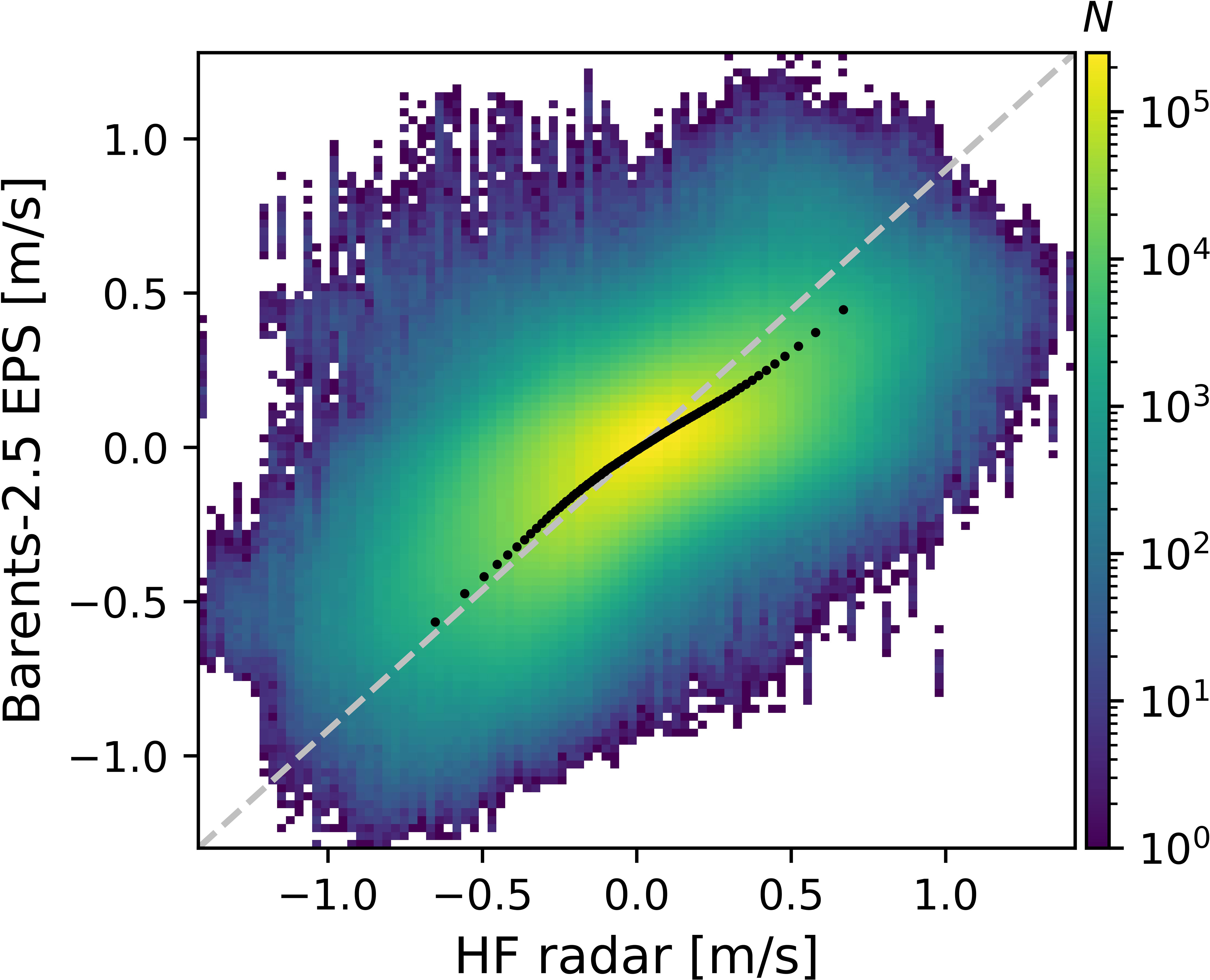
Figure 2 2D histogram and quantile-quantile plot of modeled versus observed radial current components. Barents-2.5 EPS radial velocities are shown on the vertical axis and HF radar radial velocities on the horizontal axis. N is the number of data points within each bin. The data cover the period 2021-11-15–2021-12-31.

Figure 3 shows model validation statistics as a function of lead time. In comparison to HF radar observations, all members show a mean spatial correlation of 0.53, 0.52, and 0.51 for forecast lead times +24h, +48h, and +66h, respectively. The mean bias is approximately 2.6 cm/s for all lead times over all EPS members. Regarding MAE and RMSE over all members, they are respectively about 15.6 cm/s and 20.3 cm/s for +24h, and growing almost linearly with time to approximately 15.9 cm/s and 20.6 cm/s for +66h. In general, the mean spatial correlation decreases slightly with increasing lead time; both mean RMSE and mean MAE increase with increasing lead time. Considering only high-resolution members forced by AROME-Arctic (dashed orange lines in Figure 3), there is a tendency that mean RMSE and mean MAE are lower for all lead times; no significant changes are notable in the mean spatial correlation. This suggests that high-resolution wind forcing (2.5 km resolution instead of around 10 km in the IFS) provides better forecast skill relative to the analysis when considering surface currents. Due to strong current signals along the coast and the model being constrained by the coastline, the agreement between observations and model is good. Winds are updated for each forecast cycle in the model, maintaining the model performance over short lead times. Sea surface temperature is assimilated in Barents-2.5 EPS, which to a certain degree supports the prediction of surface currents on meso and larger scales. E.g., sea surface temperature could constrain the position of the NCC and larger, long-lived eddy structures. Another constraint for the model is prescribed by the bathymetry and coastline. Hence, it is expected that the model performance might vary for other HF radar locations and for different areas, e.g. the open ocean where HF radar measurements are typically not available.

FIGURE 3

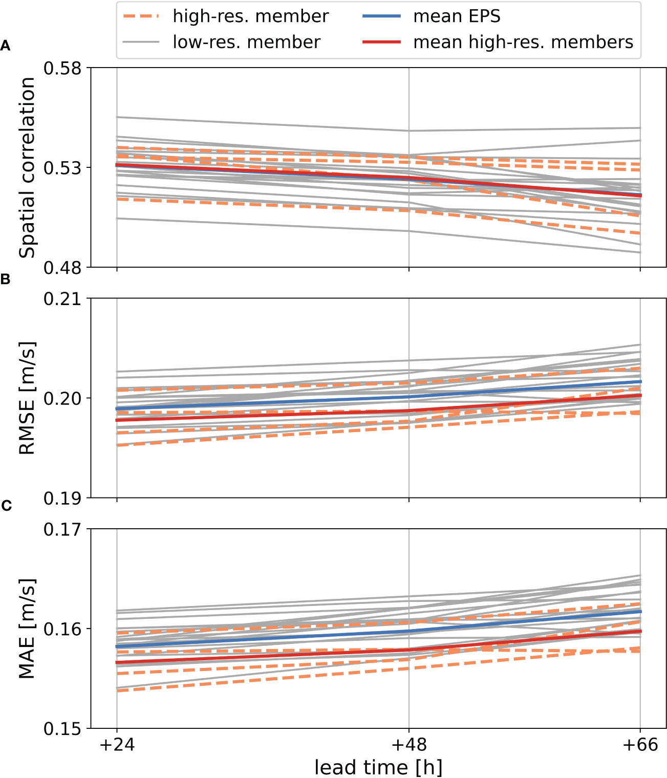
Figure 3 (A) Spatial correlation, (B) root-mean-square error, and (C) mean absolute error between surface currents from HF radar and 24 Barents-2.5 EPS members shown as a function of lead time for the period 2021-11-15–2021-12-31. Solid gray lines represent statistics of members forced by IFS atmospheric files (low-resolution member). Dashed orange lines are ensemble members forced by the AROME-Arctic weather model (high-resolution member). Solid blue and red lines represent mean values of all 24 members and of four high-resolution members, respectively.

3.2 Prediction of uncertainty in surface currents

Figures 4A, B show reliability diagrams for two forecast lead times and for events that the radial current component exceeds 0.1 m/s, 0.2 m/s, 0.3 m/s, and 0.4 m/s. Overall, the model underestimates low probabilities and overestimates high probabilities. For low values of the radial current component, the model is more reliable when it comes to high probabilities. When looking at more extreme values of the radial current component, we note more of a linear behavior in the reliability, but lack the extremes in high probabilities. For surface currents above 0.3 m/s, when the model predicts a 90% probability of occurrence we see that the observed speeds exceed this threshold in only 75% of the same cases. Further, around 20% of the cases with predicted forecast probability of 20% are observed to pass the threshold of 0.3 m/s. The biggest discrepancy is for low current speeds: when the model predicts a 20% chance to exceed 0.1 m/s, more than 45% of the observed cases exceed the threshold. The inclusion of the total observation error has a large impact, specifically on low forecast probabilities for all thresholds. The “inverted S-shaped” curves in Figures 4A, B are characteristic for ensembles with too little spread.

FIGURE 4

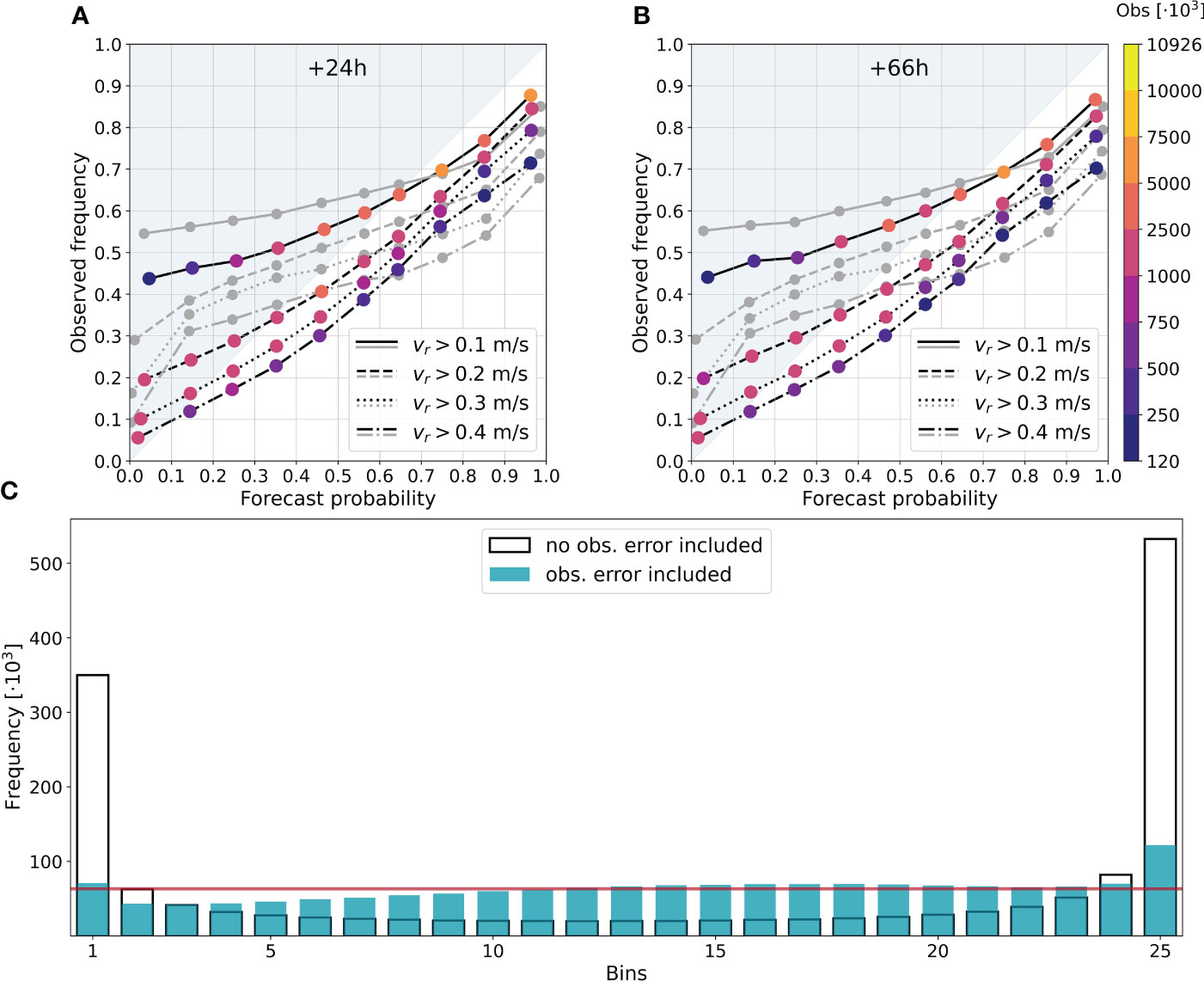
Figure 4 (A, B) Reliability diagrams for two forecast lead times for all observation points combined within the period 2021-11-15–2021-12-31. Solid, dashed, dotted, and dash-dotted lines of reliability diagrams show forecast reliability for the observed absolute radial current component for thresholds above 0.1 m/s, 0.2 m/s, 0.3 m/s, and 0.4 m/s, respectively. The horizontal axis is the forecast probability between 0 and 1 from the EPS, and the vertical axis indicates the corresponding observed frequency of occurrence. The different colors indicate the number of observations that exceeded the given threshold for a given forecast probability. (C) Rank histograms for all observed locations within the above mentioned period. The forecast lead time of +24h is shown here. Observation rank is given along the horizontal axis and frequencies along the vertical axis. The red horizontal line indicates frequencies for an unbiased ensemble. For black lines in (A, B) as well as the blue bars in (C), a normal distributed random error with a standard deviation based on the total observation error, σ_total, was added to all ensemble members (see Section 2.1).

The original and the corrected rank histograms presented in Figure 4C indicate that the distribution appearing to result from a lack of ensemble spread can be explained by observation errors. The corrected graph shows a mostly flat distribution of observations within the ensemble, which confirms that each member has a nearly equal likelihood of occurrence. Possible reasons for the remaining lack of extreme velocities, apart from insufficient ensemble spread, is limited model resolution, lack of detail in the air-sea coupling in the model, and spurious numerical diffusion. Rank histograms for lead times from +24h to +66h do not significantly differ, indicating that ensemble spread is maintained in the full forecast range.

A degree of model constraint is given by boundary conditions - through atmospheric forcing and lateral constraints such as coastlines and bathymetry. Kim et al. (2009) show that the wind driven ocean circulation is fairly well predictable when initial conditions are readily known. In addition, we argue that a degree of predictability may already be achieved when lateral boundaries, bathymetry, and wind-driven currents are a substantial part of the total current. Also tidal and large scale circulation are already well described in operational ocean models (Röhrs et al., 2023b). In fact, Khade et al. (2017) find that forecast uncertainties in coastal regions in the Gulf of Mexico are dominated by wind forcing rather than by initial conditions. This is partly reflected in our study, as we identify better forecast skill for short lead times, i.e. deteriorating skill in the forecast range relative to the analysis. Close to the analysis time, the model benefits from updated wind forcing. In addition, we see that high-resolution wind forcing (AROME-Arctic) provides improved forecast skill relative to the analysis, resulting in lower errors (Figure 3).

4 Concluding remarks on regional ocean modeling

Ensemble ocean forecasting from high-resolution coastal models has great potential, e.g. in providing uncertainties in drift modeling and for near-real-time decision making in maritime operations that are affected by currents. The predicted probability for critical conditions, such as surface current speeds above a given threshold, can be taken into account in the planning phase and during operations. Exact forecasts of current speed and direction remain unfeasible due to the lack of predictive skill in high-resolution ocean models. However, the ability to identify highly probable situations from the model ensemble is what gives the inherent usefulness of a well-balanced ocean EPS.

In this work, we have shown promising abilities of a regional ocean ensemble for the Barents Sea to predict surface currents and their uncertainty in the Norwegian coastal zone. The spatial correlation between observed and modeled surface current speeds shows a decreasing trend with increasing lead time; both mean RMSE and mean MAE increase. Barents-2.5 EPS demonstrates to have statistic skill, by providing the right magnitudes of radial components of surface currents, but has low predictive skill. The reliability diagrams as well as rank histograms show an absence of extreme events in the surface current field, which in turn indicates a lack of spread in the ensemble. Although the spread appears insufficient, the EPS maintains the same spread and ensemble reliability over its full forecast range.

In regional ocean modeling, in addition to initial conditions, both lateral constraints and atmospheric forcing at the surface are necessary to predict surface current fields (Kim et al., 2009). We want to stress that the initial conditions exhibit large uncertainty, as no direct assimilation of currents takes place in the herein considered model. In situations when coastlines, bathymetry, and wind-driven currents are significant parts of the total current, a degree of predictability seems to be achieved without direct assimilation of currents. We confirm similar findings of Cucco et al. (2016), seeing that ensemble members with higher resolution wind forcing provide a better forecast skill in surface currents relative to the analysis. The generally higher skill of atmospheric weather prediction models compared to OGCMs propagates into the forecast skill for coastal currents, particularly for situations of strong surface currents driven by wind events.

In order to assimilate surface currents from HF radars and/or satellite altimetry using variational or ensemble methods, a precondition is to have statistical skill and bias-free background state (Evensen, 1994; Moore et al., 2011). With statistic skill in surface currents from an OGCM already present, higher predictive skill is expected to result from assimilation of observations that constrain current fields on local scales. In addition, observations of the density – salinity and temperature – at depth help to prescribe density fields that control the ocean’s baroclinic response to forcing. Concurrent assimilation of both current and density fields has been shown to greatly improve surface currents (Sperrevik et al., 2015) and in particular Lagrangian drift trajectories (Sperrevik et al., 2017). Combining those information will profoundly improve predictive skill in surface currents on the regional scale in the near future.

Data availability statement

The datasets presented in this study can be found in online repositories. The names of the repository/repositories and accession number(s) can be found in the article.

Author contributions

MI, ER, and JR contributed to conception and design of the study. MI designed the computational framework and analyzed the data. MI wrote the manuscript with input from ER and JR. JR supervised the work. All authors contributed to the article and approved the submitted version.

Funding

This work has been funded by the Research Council of Norway through grants 237906 (CIRFA) and 300329 (Ecopulse).

Acknowledgments

We would like to thank the two reviewers for helpful comments that greatly improved the manuscript.

Conflict of interest

The authors declare that the research was conducted in the absence of any commercial or financial relationships that could be construed as a potential conflict of interest.

Publisher’s note

All claims expressed in this article are solely those of the authors and do not necessarily represent those of their affiliated organizations, or those of the publisher, the editors and the reviewers. Any product that may be evaluated in this article, or claim that may be made by its manufacturer, is not guaranteed or endorsed by the publisher.

References

Barrick D. E., Weber B. L. (1977). On The Nonlinear Theory for Gravity Waves on the Ocean’s Surface. Part II: Interpretation and Applications. J. Phys. Oceanogr. 7, 11–21. doi: 10.1175/1520-0485(1977)007<0011:OTNTFG>2.0.CO;2

CrossRef Full Text | Google Scholar

Barth A., Alvera-Azcárate A., Weisberg R. H. (2008). Assimilation of high-frequency radar currents in a nested model of the West Florida Shelf. J. Geophys. Res.: Oceans 113, C08033. doi: 10.1029/2007JC004585

CrossRef Full Text | Google Scholar

Christensen K. H., Breivik O., Dagestad K. F., Röhrs J., Ward B. (2018). Short-Term Predictions of Oceanic Drift. Oceanography 31, 59–67. doi: 10.5670/oceanog.2018.310

CrossRef Full Text | Google Scholar

Cosoli S., Mazzoldi A., Gačić M. (2010). Validation of Surface Current Measurements in the Northern Adriatic Sea from High-Frequency Radars. J. Atmospheric Oceanic Technol. 27, 908–919. doi: 10.1175/2009JTECHO680.1

CrossRef Full Text | Google Scholar

Cucco A., Quattrocchi G., Satta A., Antognarelli F., De Biasio F., Cadau E., et al. (2016). Predictability of wind-induced sea surface transport in coastal areas. J. Geophys. Res.: Oceans 121, 5847–5871. doi: 10.1002/2016JC011643

CrossRef Full Text | Google Scholar

Dagestad K. F., Röhrs J. (2019). Prediction of ocean surface trajectories using satellite derived vs. modeled ocean currents. Remote Sens. Environ. 223, 130–142. doi: 10.1016/j.rse.2019.01.001

CrossRef Full Text | Google Scholar

De Dominicis M., Bruciaferri D., Gerin R., Pinardi N., Poulain P. M., Garreau P., et al. (2016). A multi-model assessment of the impact of currents, waves and wind in modelling surface drifters and oil spill. Deep-Sea Res. Pt. II 133, 21–38. doi: 10.1016/j.dsr2.2016.04.002

CrossRef Full Text | Google Scholar

Evensen G. (1994). Inverse methods and data assimilation in nonlinear ocean models. Physica D: Nonlinear Phenomena 77, 108–129. doi: 10.1016/0167-2789(94)90130-9

CrossRef Full Text | Google Scholar

Fritzner S. M., Graversen R., Christensen K. H., Rostosky P., Wang K. (2019). Impact of assimilating sea ice concentration, sea ice thickness and snow depth in a coupled ocean-sea ice modelling system. Cryosphere 13, 491–509. doi: 10.5194/tc-13-491-2019

CrossRef Full Text | Google Scholar

Fritzner S. M., Graversen R. G., Wang K., Christensen K. H. (2018). Comparison between a multi-variate nudging method and the ensemble kalman filter for sea-ice data assimilation. J. Glaciol. 64, 387–396. doi: 10.1017/jog.2018.33

CrossRef Full Text | Google Scholar

Gopalakrishnan G., Blumberg A. F. (2012). Assimilation of HF radar-derived surface currents on tidal-timescales. J. Operational Oceanogr. 5, 75–87. doi: 10.1080/1755876X.2012

CrossRef Full Text | Google Scholar

Gough M. K., Garfield N., McPhee-Shaw E. (2010). An analysis of HF radar measured surface currents to determine tidal, wind-forced, and seasonal circulation in the Gulf of the Farallones, California, United States. J. Geophys. Res.: Oceans 115, C04019. doi: 10.1029/2009JC005644

CrossRef Full Text | Google Scholar

Gurgel K.-W., Dzvonkovskaya A., Pohlmann T., Schlick T., Gill E. (2011). Simulation and detection of tsunami signatures in ocean surface currents measured by HF radar. Ocean Dynam. 61, 1495–1507. doi: 10.1007/s10236-011-0420-9

CrossRef Full Text | Google Scholar

Hamill T. M. (2001). Interpretation of Rank Histograms for Verifying Ensemble Forecasts. Monthly Weather Rev. 129, 550–560. doi: 10.1175/1520-0493(2001)129<0550:IORHFV>2.0.CO;2

CrossRef Full Text | Google Scholar

Hernandez-Lasheras J., Mourre B., Orfila A., Santana A., Reyes E., Tintoré J. (2021). Evaluating high-frequency radar data assimilation impact in coastal ocean operational modelling. Ocean Sci. 17, 1157–1175. doi: 10.5194/os-17-1157-2021

CrossRef Full Text | Google Scholar

Idžanović M., Ophaug V., Andersen O. (2017). The coastal mean dynamic topography in Norway observed by CryoSat-2 and GOCE. Geophys. Res. Lett. 44, 5609–5617. doi: 10.1002/2017GL073777

CrossRef Full Text | Google Scholar

Isern-Fontanet J., Ballabrera-Poy J., Turiel A., García-Ladona E. (2017). Remote sensing of ocean surface currents: a review of what is being observed and what is being assimilated. Nonlinear Processes Geophys. 24, 613–643. doi: 10.5194/npg-24-613-2017

CrossRef Full Text | Google Scholar

Jacobs G., D’Addezio J. M., Ngodockm H., Souopgui I. (2021). Observation and model resolution implications to ocean prediction. Ocean Modeling 159, 101760. doi: 10.1016/j.ocemod.2021.101760

CrossRef Full Text | Google Scholar

Jacobs G., Richman J. G., Doyle J. D., Spence P. L., Bartels B. P., Barron C. N., et al. (2014). Simulating conditional deterministic predictability within ocean frontogenesis. Ocean Modeling 78, 1–16. doi: 10.1016/j.ocemod.2014.02.004

CrossRef Full Text | Google Scholar

Khade V., Kurian J., Chang P., Szunyogh I., Thyng K., Montuoro R. (2017). Oceanic ensemble forecasting in the Gulf of Mexico: An application to the case of the Deep Water Horizon oil spill. Ocean Model. 113, 171–184. doi: 10.1016/j.ocemod.2017.04.004

CrossRef Full Text | Google Scholar

Kim S., Samelson R. M., Snyder C. (2009). Ensemble-Based Estimates of the Predictability of Wind-Driven Coastal Ocean Flow over Topography. Monthly Weather Rev. 137, 2515–2537. doi: 10.1175/2009MWR2631.1

CrossRef Full Text | Google Scholar

Kirincich A. R., Lentz S. J., Farrar J. T., Ganju N. K. (2013). The Spatial Structure of Tidal and Mean Circulation over the Inner Shelf South of Martha's Vineyard, Massachusetts. J. Phys. Oceanogr. 43, 1940–1958. doi: 10.1175/JPO-D-13-020.1

CrossRef Full Text | Google Scholar

Køltzow M., Casati B., Bazile E., Haiden T., Valkonen T. (2019). An NWP Model Intercomparison of Surface Weather Parameters in the European Arctic during the Year of Polar Prediction Special Observing Period Northern Hemisphere 1. Weather Forecasting 34, 959–983. doi: 10.1175/WAF-D-19-0003.1

CrossRef Full Text | Google Scholar

Laws K. E., Vesecky J. F., Paduan J. D. (2011). “Error assessment of HF radar-based ocean current measurements: An error model based on sub-period measurement variance,” in 2011 IEEE/OES 10th Current, Waves and Turbulence Measurements (CWTM) IEEE, Monterey, CA, USA. 70–76. doi: 10.1109/CWTM.2011.5759527

CrossRef Full Text | Google Scholar

Lima L. N., Pezzi L. P., Penny S. G., Tanajura C. A. S. (2019). An investigation of Ocean Model Uncertainties Through Ensemble Forecast Experiments in the Southwest Atlantic Ocean. J. Geophys. Res.: Oceans 124, 432–452. doi: 10.1029/2018JC013919

CrossRef Full Text | Google Scholar

Lorenz E. N. (1969). The predictability of a flow which possesses many scales of motion. Tellus 21, 289–307. doi: 10.3402/tellusa.v21i3.10086

CrossRef Full Text | Google Scholar

Moore A. M., Arango H. G., Broquet G., Edwards C., Veneziani M., Powell B., et al. (2011). The Regional Ocean Modeling System (ROMS) 4-dimensional variational data assimilation systems: Part III – Observation impact and observation sensitivity in the California Current System. Prog. Oceanogr. 91, 74–94. doi: 10.1016/j.pocean.2011.05.005

CrossRef Full Text | Google Scholar

Müller M., Homleid M., Ivarsson K.-I., Køltzow M. A., Lindskog M., Midtbø K. H., et al. (2017). AROME-MetCoOp: A Nordic Convective-Sale Operational Weather Prediction Model. Weather Forecasting 32, 609–627. doi: 10.1175/WAF-D-16-0099.1

CrossRef Full Text | Google Scholar

Nonaka M., Sasai Y., Sasaki H., Taguchi B., Nakamura H. (2016). How potentially predictable are midlatitude ocean currents? Sci. Rep. 6, 20153. doi: 10.1038/srep20153

PubMed Abstract | CrossRef Full Text | Google Scholar

Oke P. R., Allen J. S., Miller R. N., Egbert G. D., Kosro P. M. (2002). Assimilation of surface velocity data into a primitive equation coastal ocean model. J. Geophys. Res.: Oceans 107, 5–1–5–25. doi: 10.1029/2000JC000511

CrossRef Full Text | Google Scholar

Pinardi N., Bonazzi A., Dobricic S., Milliff R. F., Wikle C. K., Berliner L. M. (2011). Ocean ensemble forecasting. Part II: Mediterranean Forecast System response. Q. J. R. Meteorological Soc. 137, 879–893. doi: 10.1002/qj.816

CrossRef Full Text | Google Scholar

Prasad S. J., Balakrishnan Nair T. M., Balaji B. (2022). Improved prediction of oil drift pattern using ensemble of ocean currents. J. Operational Oceanogr. 0, 1–16. doi: 10.1080/1755876X.2022.2147699

CrossRef Full Text | Google Scholar

Röhrs J., Gusdal Y., Rikardsen E. S. U., Moro M. D., Brændshøi J., Kristensen N. M., et al. (2023a). Barents-2.5km v2.0: An operational data-assimilative coupled ocean and sea ice ensemble prediction model for the Barents Sea and Svalbard. In Rev. Geoscientific Model. Dev. doi: 10.5194/gmd-2023-20

CrossRef Full Text | Google Scholar

Röhrs J., Sutherland G., Jeans G., Bedington M., Sperrevik A. K., Dagestad K.-F., et al. (2023b). Surface currents in operational oceanography: Key applications, mechanisms, and methods. J. Operational Oceanogr. 16, 60–88. doi: 10.1080/1755876X.2021.1903221

CrossRef Full Text | Google Scholar

Saetra O., Hersbach H., Bidlot J.-R., Richardson D. S. (2004). Effects of Observation Errors on the Statistics for Ensemble Spread and Reliability. Monthly Weather Rev. 132, 1487–1501. doi: 10.1175/1520-0493(2004)132<1487:EOOEOT>2.0.CO;2

CrossRef Full Text | Google Scholar

Sandery P. A., Sakov P. (2017). Ocean forecasting of mesoscale features can deteriorate by increasing model resolution towards the submesoscale. Nat. Commun. 8, 1566. doi: 10.1038/s41467-017-01595-0

PubMed Abstract | CrossRef Full Text | Google Scholar

Shay L. K., Graber H. C., Ross D. B., Chapman R. D. (1995). Mesoscale Ocean Surface Current Structure Detected by High-Frequency Radar. J. Atmospheric Oceanic Technol. 12, 881–900. doi: 10.1175/1520-0426(1995)012<0881:MOSCSD>2.0.CO;2

CrossRef Full Text | Google Scholar

Shchepetkin A. F., McWilliams J. C. (2005). The regional oceanic modeling system (ROMS): a splitexplicit, free-surface, topography-following-coordinate oceanic model. Ocean Model. 9, 347–404. doi: 10.1016/j.ocemod.2004.08.002

CrossRef Full Text | Google Scholar

Sperrevik A. K., Christensen K. H., Röhrs J. (2015). Constraining energetic slope currents through assimilation of high-frequency radar observations. Ocean Sci. 11, 237–249. doi: 10.5194/os-11-237-2015

CrossRef Full Text | Google Scholar

Sperrevik A. K., Röhrs J., Christensen K. H. (2017). Impact of data assimilation on Eulerian versus Lagrangian estimates of upper ocean transport. J. Geophys. Res.: Oceans 122, 5445–5457. doi: 10.1002/2016JC012640

CrossRef Full Text | Google Scholar

Stewart R. H., Joy J. W. (1974). HF radio measurements of surface currents. Deep Sea Res. Oceanographic Abstracts 21, 1039–1049. doi: 10.1016/0011-7471(74)90066-7

CrossRef Full Text | Google Scholar

Strand K. Ø., Breivik O., Pedersen G., Vikebø F. B., Sundby S., Christensen K. H. (2020). Long-Term Statistics of Observed Bubble Depth Versus Modeled Wave Dissipation. J. Geophys. Res.: Oceans 125, e2019JC015906. doi: 10.1029/2019JC015906

CrossRef Full Text | Google Scholar

Thoppil P. G., Frolov S., Rowley C. D., Reynolds C. A., Jacobs G. A., Joseph Metzger E., et al. (2021). Ensemble forecasting greatly expands the prediction horizon for ocean mesoscale variability. Commun. Earth Environ. 2, 89. doi: 10.1038/s43247-021-00151-5

CrossRef Full Text | Google Scholar

Tilmann G., Raftery A. E. (2005). Weather Forecasting with Ensemble Methods. Science 310, 248–249. doi: 10.1126/science.1115255

PubMed Abstract | CrossRef Full Text | Google Scholar

Umlauf L., Burchard H. (2005). Second-order turbulence closure models for geophysical boundary layers. A review of recent work. Continental Shelf Res. 25, 795–827. doi: 10.1016/j.csr.2004.08.004

CrossRef Full Text | Google Scholar

Vignudelli S., Birol F., Benveniste J., Fu L.-L., Picot N., Raynal M., et al. (2019). Satellite Altimetry Measurements of Sea Level in the Coastal Zone. Surveys Geophys. 40, 1319–1349. doi: 10.1007/s10712-019-09569-1

CrossRef Full Text | Google Scholar

Wilks D. S. (2019). Statistical methods in the atmospheric sciences. Fourth Edition. (Amsterdam, Netherlands: Elsevier).

Google Scholar

WMO (2012). Guidelines on Ensemble Prediction Systems and Forecasting (Report WMO-No. 1091). World Meteorological Organization.

Google Scholar