 Allison L. White
- 1Marine Ecology and Acoustics Laboratory, Department of Biology, Florida International University, North Miami Beach, FL, United States
- 2Department of Natural Resources, Cornell University, Ithaca, NY, United States
“Star” survey designs have become an increasingly popular alternative to parallel line designs in fisheries-independent sampling of areas with isolated fish aggregations, such as artificial reefs, seamounts, fish aggregating devices, and spawning aggregation sites. In this study, we simulated three scenarios of fish aggregating around a feature of interest with variations in the size and complexity of aggregations as well as their location relative to the habitat feature. Simulated and empirical data representing goliath grouper (Epinephalus itajara) spawning aggregations at artificial reefs were utilized as a case study, and scenarios were generated in relation to both a single habitat feature and a reef complex with multiple structures. Seven variations of survey design using both star and parallel transects were examined and compared by geostatistical and generalized additive models (GAMs) to identify the most robust approach to quantify fish aggregations in each scenario. In most scenarios, precision in the mean and variability of backscatter estimates is not significantly affected by the number of transects passing over the habitat feature as long as at least one pass is made. Estimation error is minimized using the GAM approach, and is further reduced when sampling variance is high, which was better accomplished by parallel designs overall. These results will help inform surveyors on the best overall approach to improve precision in quantifying fish aggregations given basic knowledge of their behavior around an established habitat feature and help them to adapt their survey designs based on common difficulties in sampling these populations simulated below.
1 Introduction
Many fish species aggregate to spawn and/or associate with conspicuous habitat features such as seamounts and artificial reefs (Doonan et al., 2003). These sites are of great interest among fisheries scientists and managers, as fish which aggregate in highly localized and predictable areas (especially when associated with established bottom features) may be susceptible to higher catchability (Hieu et al., 2014). Continuous mobile surveys, such as those performed by towed active acoustics or camera systems, are often the optimal method to provide fisheries-independent inferences about the size of such highly localized fish aggregations. Although mobile surveys allow for ensured sampling over the discrete aggregation of interest, this inherently negates randomness in the survey design. Design-based methods of population inference, which are based on the distribution of all possible estimates within a survey design, are therefore not ideal, and surveyors of such aggregations often rely on model-based estimations of population size (Neyman, 1934; Jolly and Hampton, 1990; Gregoire, 1998; Rivoirard et al., 2000; Chang et al., 2017).
Two commonly used survey designs for mobile surveys of highly localized fish aggregations are parallel line and star designs (Figures 1A, B). Parallel line designs consist of either randomly- or evenly-spaced parallel transects. This design allows for stratified randomization by incorporating random-spacing between transects and/or randomly selecting the starting point (Jolly and Hampton, 1990). In the case of highly localized aggregations, however, evenly-spaced parallel transects are generally preferred in order to maximize the number of passes over the aggregation and starting points are selected in relation to the location of the aggregation or habitat feature (e.g. Taylor et al., 2006; Boswell et al., 2010; Kang et al., 2011).

Figure 1 (A) Parallel line survey designs and (B) star survey designs plotted over the sunken barge (grey shaded area) at MG111. Dashed lines represent turns made between transects (solid lines) which were excluded from analysis.
Though parallel line surveys offer better coverage of the area surrounding a fish aggregation and less spatial autocorrelation between transect nodes, they often involve a greater number of transects and present several practical difficulties in maneuvering tight turns. Star surveys involve fewer transects which are arranged in alternating directions and which all cross at the center of the aggregation site. Star designs may be easier to maneuver and provide a higher sampling of the targeted aggregation per survey effort, but they have an inherently large spatial autocorrelation between transect nodes (i.e., the point at which transects bisect one another). They also offer poor coverage of the area surrounding the habitat feature of interest, which results in a decreased ability to measure variability in population estimates. Despite these downfalls, star designs have increased in popularity in recent years due to the reduction in time required to obtain multiple passes over the aggregation of interest. Many surveyors believe that they can reduce the cost of vessel time and/or maximize the number of surveys conducted by employing star designs over parallel designs. Here, we weigh the advantage of cost/time reduction against decreased precision in population estimates through comparison of model-based inferences from both survey designs.
Model-based inferences do not require random sampling, and are therefore less heavily influenced by the high spatial sampling autocorrelation inherent in both parallel line and star surveys. Unlike design-based approaches, however, model-based approaches are strongly dependent on assumptions about the underlying distribution and structure of a population (Gregoire, 1998). Geostatistical models, for example, assume that the spatial distribution of the population is stationary and isotropic. In stationary populations, the statistical properties of the population do not change across time or space, and in isotropic populations the correlation between any two observations depends solely on the distance between them regardless of their relative orientation. Live fish aggregations may not fulfill either of these assumptions, resulting in biased estimations of population size. A further complication with continuous data of fish aggregations is the high proportion of zero observations. Most models, geostatistical or non-geostatistical, do not perform well on highly skewed data without extraneous methods.
In this study, we evaluate the relative biases associated with different survey designs and commonly used inference approaches to quantifying goliath grouper (Epinephalus itajara) spawning aggregations over artificial reefs in Jupiter, FL. Three scenarios of the spatial distribution of goliath grouper acoustic backscatter at two artificial reefs are surveyed by multiple variations of parallel line and star designs and estimated by a geostatistical and a non-geostatistical modeling approach as well as a design-based approach (Figure 2). Understanding the spatial distribution of the underlying population is an important first step in constructing sampling designs (Gunderson, 1993). Initial surveys should be considered exploratory and aim to give context about the spatial distribution of the targeted population. The purpose of this study is to provide guidance on least-biased survey designs and inference approaches given previous knowledge about the spatial trends of fish aggregations. We also address common issues involved with surveying populations that are assumed to be densely aggregated over or around a discrete and predictable location.
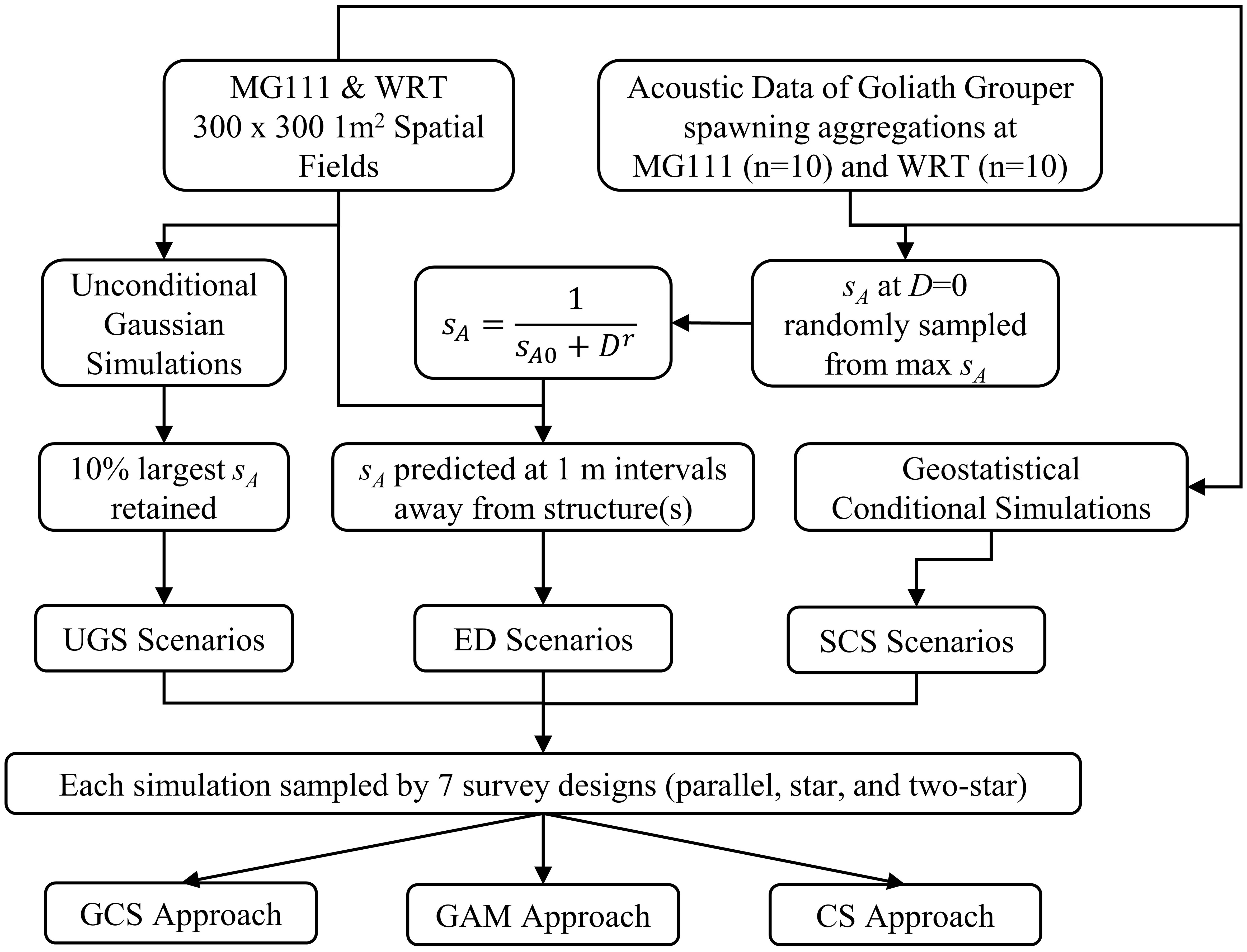
Figure 2 Flow chart showing the steps used to simulate, sample, and make inferences about sA of goliath grouper aggregations at the MG111 and WRT artificial reefs.
2 Methodology
2.1 Acoustic data collection and processing
Goliath grouper spawning aggregations were surveyed at two artificial reef complexes in Jupiter, FL. The northernmost reef complex, colloquially known as MG111, consists of the remains of a 59 m long barge resting at a depth of 18 m. A field of ~3 m tall concrete columns standing upright on the seafloor stretches north of the barge over roughly 100 x 50 m of sand. The second reef complex, colloquially known as Wreck Trek (WRT), is located ~2 km south of MG111 and includes a collection of three shipwrecks arranged north to south with a ~170 m distance between the northernmost and southernmost wrecks. The 45 m long Esso Bonaire oil tanker, 17 m long Miss Jenny barge, and the stern of the 50 m long Zion Train cargo ship all lie in 27 m of water. Both artificial reef complexes were selected for this study based on their consistent use by goliath grouper as spawning aggregation sites (Koenig et al., 2017).
Active acoustic surveys (n=10) were conducted over these reefs during goliath grouper spawning months (August through November) in 2017 and 2018. Surveys were conducted with a 38 kHz (10˚) split-beam Simrad EK80 echosounder towed at the surface ~15 m behind a 7 m research vessel. The echosounder was calibrated following the standard sphere method (38.1 mm tungsten carbide sphere with 6% cobalt binder; Demer et al., 2015). Two transect designs were conducted sequentially at each survey event: 1) a parallel line survey which consisted of 15-20 east-west parallel transects that were spaced ~20 m apart (Figure 1A); and 2) a star survey consisting of four radial transects separated by ~45˚ (Figure 1B). Transects in both survey designs were 300 m in length and centered over the main structure at each of the reef complexes.
Raw acoustic data were visualized and processed in Echoview 12.0 (Echoview Software Pty. Ltd.). Data were visually inspected to remove turns between transects and dropout from rapid speed changes. A best bottom candidate detection algorithm with an offset of 0.5 m was applied to exclude the acoustic dead zone and seafloor from analysis. Data within 5.5 m of the transducer face were excluded to eliminate transducer ringdown and near-field effects. Volume-backscattering strength (Sv; dB re 1m-1) data were thresholded at -60 dB re 1 m-1 to eliminate sources of backscatter that did not originate from swim-bladdered fish. Backscatter representing large-bodied goliath grouper was isolated by applying a -40 dB re 1 m2 threshold to the target strength (TS; dB re 1 m2) data (Binder, 2022). The areas in the TS echogram attributed to goliath grouper were then masked over the Sv echogram of swim-bladdered fish, which was used to calculate the nautical area scattering coefficient (sA; m2 nmi-2) from echo integrals in 5 m along-track x 5 m depth intervals from the best bottom candidate exclusion line (MacLennan et al., 2002). Resulting echo integrals near the surface less than 2 m in maximum height were excluded from further analysis.
The convex hull of the mean coordinates for all 5 m transect distances throughout the water column was used to generate a spatial field with a 300 m x 300 m grid of 1 m2 cells for simulation. Three scenarios of the underlying distribution of fish aggregations at the two artificial reefs were simulated across these spatial fields: an unconditional Gaussian scenario, an exponential decay scenario, and a stochastic conditional scenario (Figure 3). Each scenario included ten simulations of goliath grouper sA over each the spatial fields of MG111 and WRT.
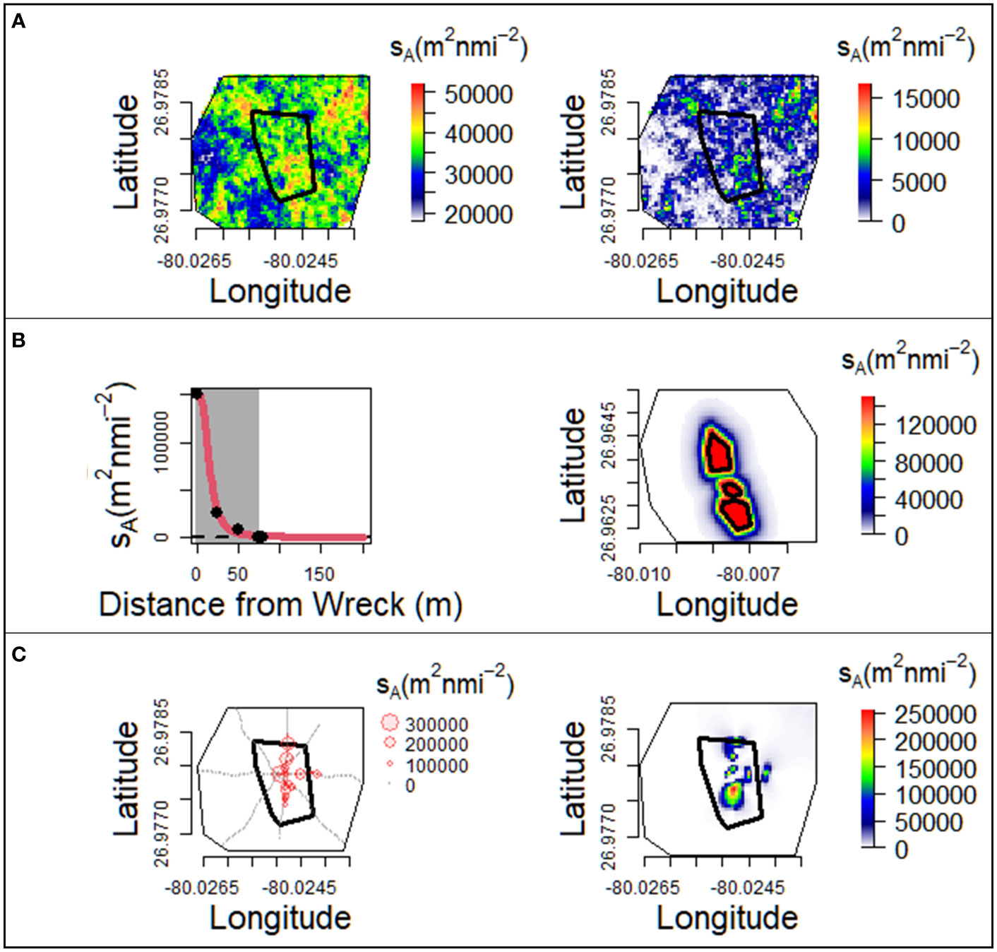
Figure 3 Construction of the three scenarios of the underlying distribution of goliath grouper aggregations. Black polygons indicate the structures at each artificial reef. Unconditional Gaussian simulations (A) were generated over the spatial fields of each wreck (left) and transformed to simulate a highly skewed population (right; MG111 shown). The exponential decay scenario (B) was built by modeling sA as a function of distance from the boundary of each structure at the two reefs (left). Maximum sA observed from acoustic surveys of goliath grouper spawning aggregations and area of influences (shown by the grey shaded region) were used to generate datasets (black filled points) fit by a non-linear regression of the exponential decay function (red line). Predicted values at 1 m distance intervals were applied to concentric polygons around the structures at each artificial reef (right; WRT shown). Stochastic conditional simulations (C) were built using sA predicted by GCS (right) of sA observed during 2017 and 2018 acoustic surveys of goliath grouper spawning aggregations (left; MG111 shown).
2.2 Unconditional Gaussian scenario
The first scenario was unconditional to the data and aimed to reflect the assumptions inherent in most modelling approaches that the underlying distribution of fish exhibits spatial independence. In this scenario, fish are randomly distributed throughout the spatial field with no correlation to any promontories. A Gaussian random field with a Matérn covariance structure was generated over the spatial fields in each simulation (Cressie, 1993). Variability in the randomness of sA distributed across the spatial field and in the size of fish aggregations were incorporated into these simulations following the method described in Chang et al. (2017). To simulate the highly skewed distribution of data present in most water column sampling methods (including active acoustics), the sA values generated by each unconditional Gaussian simulation (UGS) were subtracted by their mode and a 100 m2 nmi-2 offset. All adjusted sA values below 100 m2 nmi-2 were assigned zero values, resulting in spatial fields with 44-55% sA=0 (Figure 3A).
2.3 Exponential decay scenario
The second scenario was simulated to reflect the assumption that fish backscatter is highest directly over promontories and exhibits an exponential decay in every direction away from the boundaries of the structure. In this scenario, goliath grouper sA was modelled at increasing distances away from the boundaries of the main structures in each reef complex following the exponential decay (ED) function:
where goliath grouper sA is a function of the reciprocal of the goliath grouper backscatter directly over the structure sA0 as it decays at rate r with increasing distance D (m) away from the boundary of the structure. A dataset was generated for each simulation with eight observations: 1) the maximum sA at D = 0 (randomly sampled from maximum goliath grouper sA observed from all processed acoustic surveys); 2) the minimum distance where sA = 0 to represent the area of influence around the artificial structure (randomly sampled between 35 and 179 m as estimated by White et al., 2022); and 3-8) six sequential distances at 10 m intervals greater than the area of influence where sA = 0 to represent the horizontal asymptote in goliath grouper backscatter. Nonlinear least squares regression models were used to fit the exponential decay function (Eq. 1) to these generated datasets (Bates and Watts, 1988). The predicted sA at each 1 m distance away from the structures were then attributed to concentric polygons drawn at 1 m intervals away from the boundary of the main structure across the spatial field of sA at MG111. For the three wrecks at WRT, predicted sA was attributed to concentric polygons which were drawn at 1 m intervals away from the boundaries of each of the three structures (Figure 3B). Goliath grouper sA simulated by this method had 50-78% of the observations where sA=0.
2.4 Stochastic conditional scenario
The last scenario was built upon real world acoustic data of goliath grouper spawning aggregations and was designed to incorporate the stochasticity of live fish aggregations. This stochastic conditional simulation (SCS) scenario was made to reflect the behavior of fish around a habitat feature at any given point in time, such as spawning behaviors or utilizing structures to shelter from currents, predator avoidance, varying light levels around a structure, etc. Geostatistical conditional simulations (GCS) were used to generate realizations of goliath grouper spawning events observed at MG111 and WRT (Figure 3C). These simulations produced random fields which were conditional to the sA observed during goliath grouper spawning events and highly zero-inflated (40-94% sA=0). See section 2.6 below for a more detailed description of how GCS were performed.
2.5 Survey designs
Goliath grouper sA was sampled from each simulation in the above three scenarios via seven variations in survey designs of parallel line and star transect methods (Figure 4). These designs were:
1. Ideal transects: Evenly spaced 250 m long parallel line transects (n=6 spaced 40 m apart for MG111 and n=12 spaced 20 m apart for WRT) centered so that four transects crossed over the structure at MG111 and four transects crossed over each of the Esso Bonaire and Zion Train wrecks at WRT. The ideal star design was composed of four 250 m long transects separated by 45˚ which converged over the center point of the barge at MG111 and over the center point of the three shipwrecks at WRT. An additional transect method with two stars of four 250 m long transects each was constructed at WRT with one star centered over the center point of the Esso Bonaire and one star centered over the Zion Train wreck.
2. Single offset transect: As (1) but with one transect offset over the reefs so that only three transects passed over each structure instead of the four in the ideal transects.
3. Double offset transects: As (1) but with two transects offset over the reefs so that only two transects passed over each structure.
4. Triple offset transects: As (1) but with three transects offset over the reefs so that only one transect passed over each structure.
5. Structure avoidance transects: The same number and length of transects as described in (1), but with no transects passing over the structures at each reef. For the parallel method, transects were arranged as in (1) but with transects which would have passed over the structure ending at the boundary of the structure. For the star and two-star methods, transects were arranged around the borders of the structure in order to maximize the distance along each transect which passed close to the structure (while avoiding other structures at WRT).
6. Shorter transects: Transects were arranged as in (1) but were only 150 m in length.
7. Non-uniform transects: Selected from real transects driven over MG111 and WRT. Like (1), the selected real-world transects were centered over the structures at each reef so that four transects passed over the barge at MG111 and the Esso Bonaire and Zion Train wrecks at WRT in all designs. Unlike (1), the spacing between transects varies along the transect and transect length is not exactly 250 m. Rather, all transects were cutoff at 125 m distance away from the center point of each design in every direction.
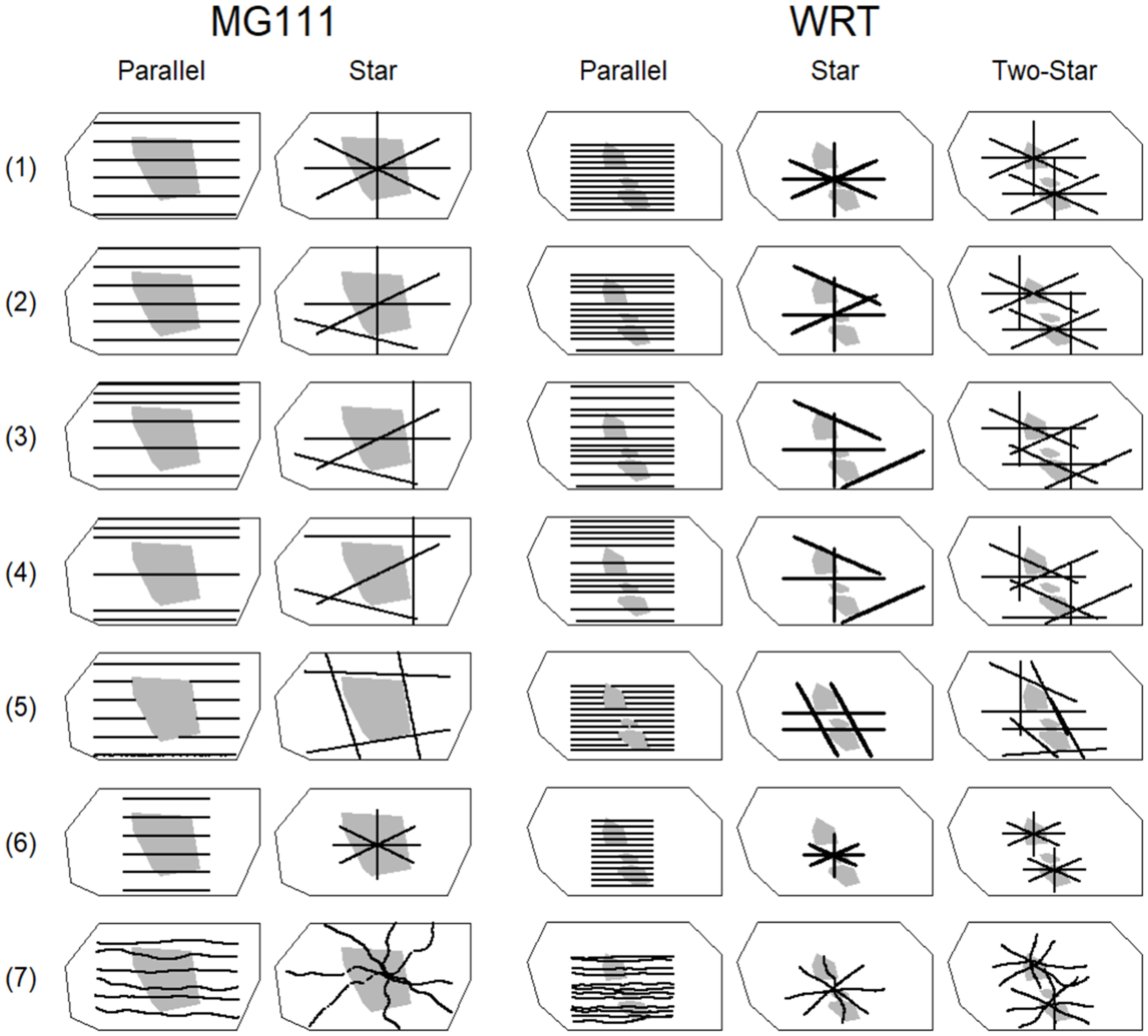
Figure 4 The seven survey designs sampled from goliath grouper sA simulated within the spatial field (outer polygon) at MG111 (left) and WRT (right). Solid black lines represent survey transects and grey shaded areas show the structure(s) at each artificial reef. Ideal transects (Design 1), single offset transects (Design 2), double offset transects (Design 3), triple offset transects (Design 4), structure avoidance transects (Design 5), shorter transects (Design 6), and non-uniform transects (Design 7) are shown for the parallel, star, and two-star methods.
The ideal transects (1) were designed to represent a scenario where the surveyor has perfect control over the placement of all transects (including vessel behavior). As this is not always possible, the remaining survey designs were compared to the ideal case in order to examine potential biases resulting from various non-ideal scenarios. Designs 2, 3, and 4 were compared to the ideal in order to estimate how much a surveyor should prioritize driving over the structure. Design 5 represents a scenario in which the surveyor is unable to drive over the aggregation of interest due to the structure extending out of the water (such as an oil rig) or high boat traffic directly over the feature of interest (which was often the case at MG111 and WRT during daylight hours). The shorter transects (6) are designed to estimate the importance of transect length away from the structure of interest. Lastly, the non-uniform transects (7) were designed to mimic situations in which the surveyor is not able to drive transects in straight lines. When towing equipment over a fish aggregation many factors may influence the path of each transect, such as strong currents, visibility, sea state, presence of other vessels, etc. Each simulation of the UGS, ED, and SCS scenarios was sampled by the seven survey designs for each of the three transect methods and input to the following modeling- and design-based approaches to estimate goliath grouper sA at the two reefs.
2.6 Inference approaches
We tested the performance of two model-based methods for spatial interpolation of goliath grouper sA: geostatistical conditional simulations (GCS) and generalized additive models (GAMs). Conditional simulations of ordinary kriging (a common geostatistical model) were selected for this study due to their ability to generate the spatial variability of population estimates while honoring the data at observed locations. While kriging allows for interpolation of data at unsampled locations (such as between transects), it also minimizes error variance (Isaaks and Srivastava, 1989). By generating multiple realizations (or simulations) of the spatial structure of the population (captured by characteristics such as the histogram and variogram), uncertainty in the global estimate of population size can be obtained. Uncertainty in global estimates was of particular concern for star survey designs, where the areas not sampled between transects increases towards the outer regions of the survey. Conditional simulations are made on the Gaussian random function model, which is not applicable to highly skewed data such as in our case. Therefore, a Gaussian anamorphosis of sA with a Gibbs sampler to iteratively simulate the points where sA = 0 was performed for all GCS following the methods described by Woillez et al. (2009; 2016). All GCS and Gaussian anamorphoses were conducted using the R package “RGeostats” (MINES ParisTech/ARMINES, 2022).
GAMs are a non-parametric regression approach capable of predicting non-linear relationships (Hastie and TibshIrani, 1990). In these models, splines are utilized to estimate smooth functions between predictor and response variables. Spatial inferences can be made by including a smooth functional relationship of the exploratory variable as a response of the interaction between latitudes and longitudes of observations. GAMs are more flexible towards non-Gaussian data than geostatistical approaches. In this study, we modelled goliath grouper sA as a function of the thin plate regression spline interaction between latitude and longitude assuming a Tweedie distribution (Wood, 2003). The Tweedie dispersion model has a non-negative support and a discrete mass at zero that makes it useful in modeling datasets with a mixture of zero and positive observations (Dunn and Smyth, 2005). GAMs were performed in R using the “mgcv” package (Wood, 2017).
In addition to the two model-based approaches described above, one design-based approach was considered. Mean goliath grouper s̄A was calculated in the surveyed space j using a cluster sampling (CS) formula (Scheaffer et al., 2012):
where s̅Ak is the average sA in transect k with n observations across all transects K. A global estimate of s̅A was interpolated by dividing the sum of observations across all transects from s̅Aj multiplied by the area of the convex hull of each survey design. Calculation of the standard deviation was adapted from Scheaffer et al. (2012) as:
2.7 Survey design and model comparison
The precisions of global estimates of the mean and coefficient of variation (CV) of sA predicted by each combination of survey design and inference approach under the three scenarios of underlying fish distribution were compared using relative mean absolute error (RMAE):
where ẑ is the predicted global estimate of the mean or CV of sA and z is the true sA value. Global estimates of ẑ were calculated from sA interpolated over the convex hull of the survey design for each inference approach, and z was calculated from the true sA generated by each simulation within the same space. Five null hypotheses (H01-5) were formally tested to compare RMAE resulting from the seven survey designs using a two-way analysis of variance (ANOVA) and Tukey’s honest significant difference (TukeyHSD) for pairwise comparisons. One ANOVA was performed for each of the three inference approaches at the two wrecks under each of the three scenarios for RMAE of the mean and of the CV, resulting in 36 models of RMAE as a function of the interactions between transect method (parallel, star, or two-star) and design (1:7). H01 was tested by comparing the difference in mean RMAE of each transect method (Designs 1-7) at each of the two artificial reefs. H02 compared errors among survey designs with differing number of transects passing over the feature of interest (Designs 1-4) for each transect method. H03 addressed the scenario in which surveying directly over the feature of interest is not possible via comparisons between Design 5 in each transect method. Precision in longer (Design 1) and shorter (Design 6) transects was compared in H04, and in H05 the precision in uniform (Design 1) and non-uniform (Design 7) transects was compared. All simulations, survey design generations, and inference approaches were performed in R (R Core Team, 2022).
3 Results
Among the three inference approaches, the design-based approach (CS) had the poorest fit (Tables 1, 2). Error in the mean and variability of sA estimated by the design approach was at least 50x larger than either of the modeling-based approaches, and is therefore not reported in the results of post hoc analyses. Both modeling approaches reproduced highly skewed distributions of sA similar to the simulated values, including a large number of zeros (Figure 5). Precision in mean sA was highest in the GAM approach, although estimation of variability in sA was equivocal between the GAM and GCS approaches (Table 1). A two-way ANOVA revealed that the relative performances of GCS versus GAMs was somewhat dependent on transect method for the estimation of sA (Table 3). Pairwise comparisons from TukeyHSD tests revealed that GAMs significantly outperformed GCS models in the estimation of mean sA at both wrecks and in the estimation of variability at MG111 regardless of transect method under the UGS scenario. In the ED scenario, however, there was no significant variation in RMAE to suggest improved performance of one model over the other when employing the two-star design. Variability of sA at MG111was better predicted by GCS than GAM, but only by the parallel transect method. In the SCS scenario, the only significant evidence of GAMs outperforming GCS models was provided when using the star design at MG111.
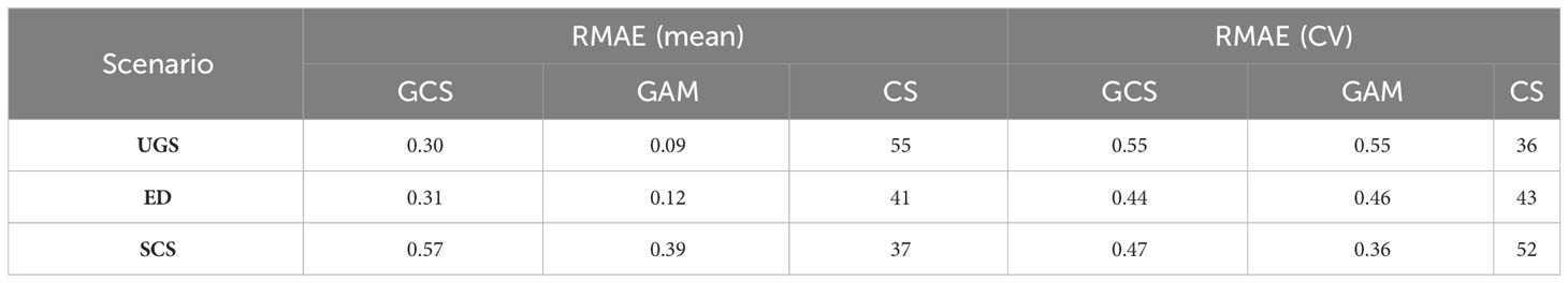
Table 1 Average RMAEs of the mean and CV sA estimated by the three inference approaches (geostatistical conditional simulations, generalized additive models, and cluster sampling).
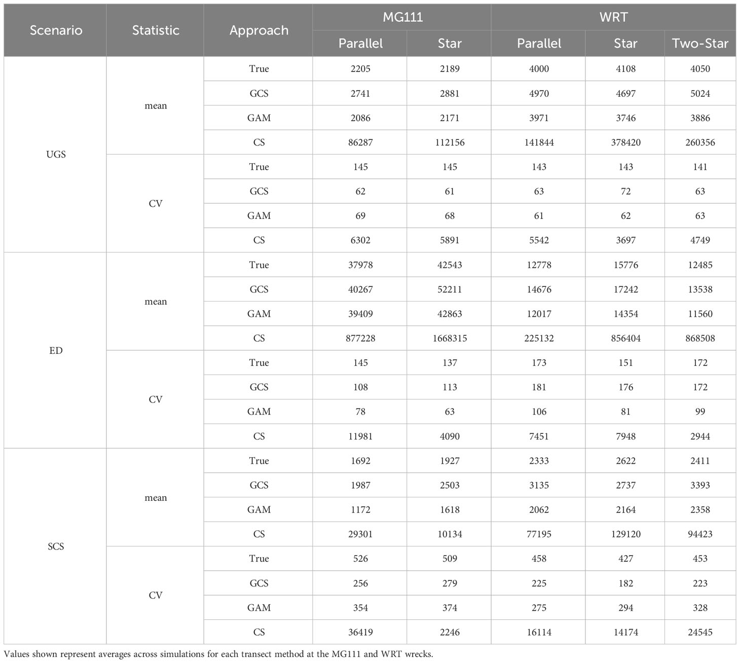
Table 2 Mean and CV of the true sA compared to sA estimated by the geostatistical conditional simulations, generalized additive models, and cluster sampling.
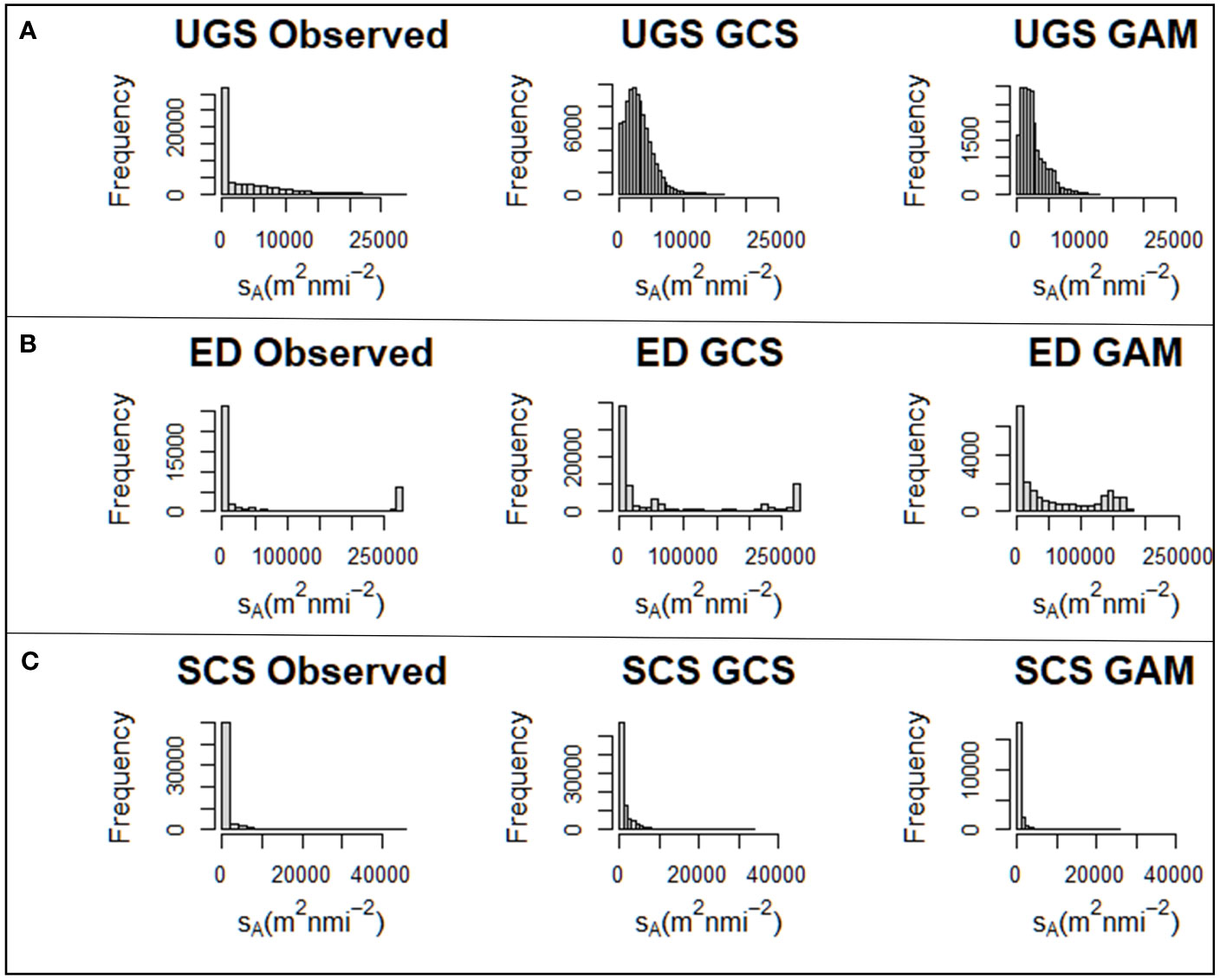
Figure 5 Example distributions of sA observed at MG111 predicted by geostatistical conditional simulations and generalized additive models in the unconditional Gaussian simulation (A), exponential decay (B), and stochastic conditional simulation (C) scenarios.

Table 3 Average RMAEs of the mean and CV sA estimated for each transect method by the geostatistical conditional simulations and generalized additive models.
Average residuals for each transect method (x̅) showed that mean sA at both wrecks was overestimated by the GCS approach and underestimated by the GAM approach for the UGS and SCS scenarios (Figure 6A; Table 2). In the ED scenario, mean sA at MG111 was overestimated by both GCS and GAM, while mean sA at WRT was underestimated by both modeling approaches. Variability in sA was underestimated by both modeling approaches in all three scenarios, with one exception (Figure 6B; Table 2). The CV of sA at WRT was overestimated by the GCS approach in the ED scenario, which was driven by an overestimation of CV in Design 5 (structure avoidance) in all transect methods.
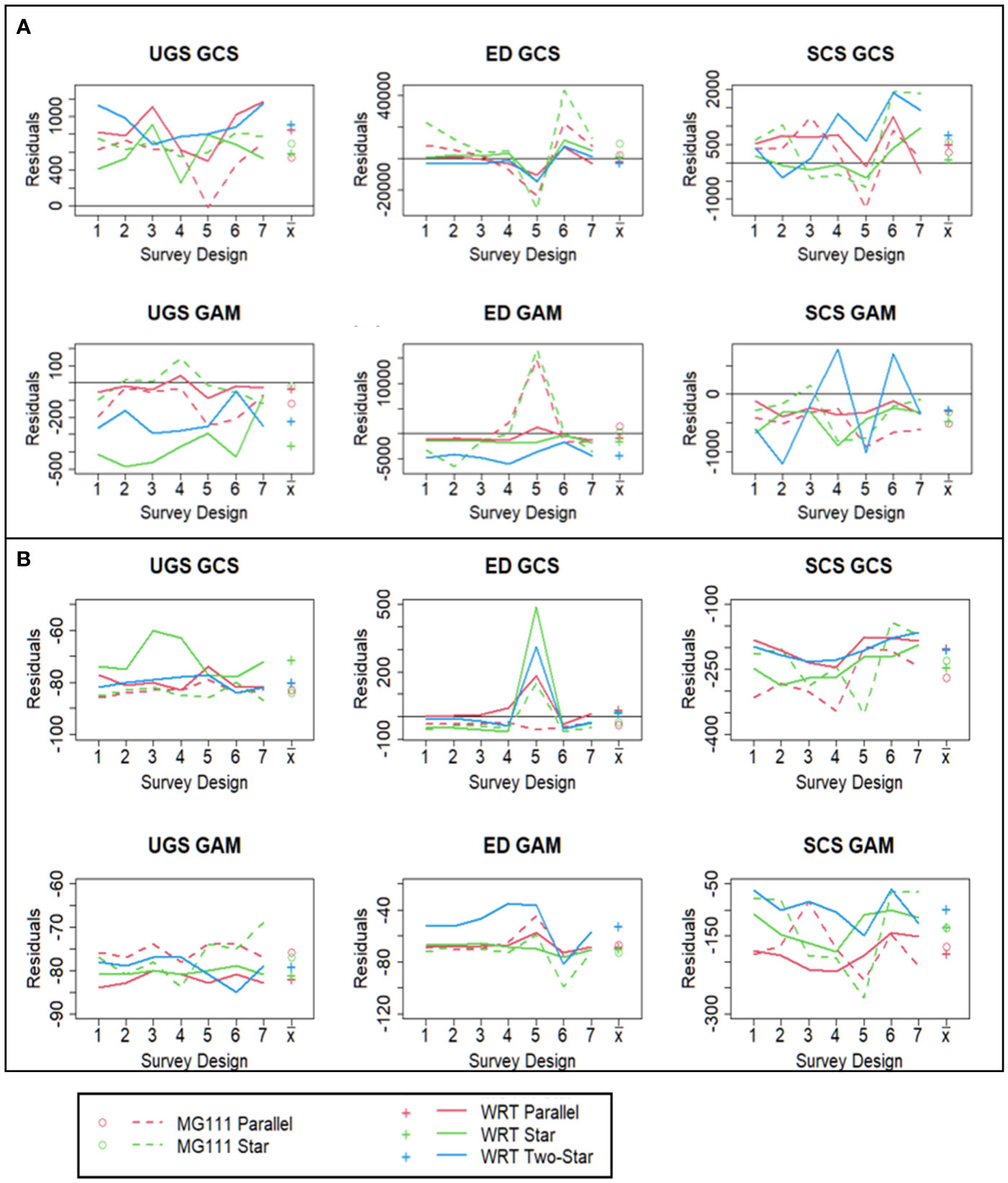
Figure 6 Average residuals of the mean (A) and CV (B) estimated by geostatistical conditional simulations and generalized additive models in each of the three scenarios sampled by the seven survey designs and the mean of each transect method (x̄).
Within survey designs, the selection of transect method (parallel, star, or two-star) was the only significant influence on model-based precision of sA estimated under all three scenarios (HA1, Table 4). In the UGS scenario, precision of variability in sA predicted by GCS was highest for the star design in comparison to both parallel and two-star designs at WRT. Parallel designs produced the least-biased estimation of mean sA at the same wreck using GAMs. Precision in the mean and CV of sA did not differ significantly between transect methods at the single structure reef using either modeling approach under this scenario. This was also true at MG111 in the SCS scenario, with the exception of the non-uniform design (7), in which the parallel method provided a better fit than the star method in the GCS estimation of mean sA. Under the SCS scenario, precision of variability in sA predicted by both GAM and GCS was lowest for the star design in comparison to both parallel and two-star designs at WRT. Mean sA from the parallel transect method was less biased than from the two-star method at WRT when using GAMs.
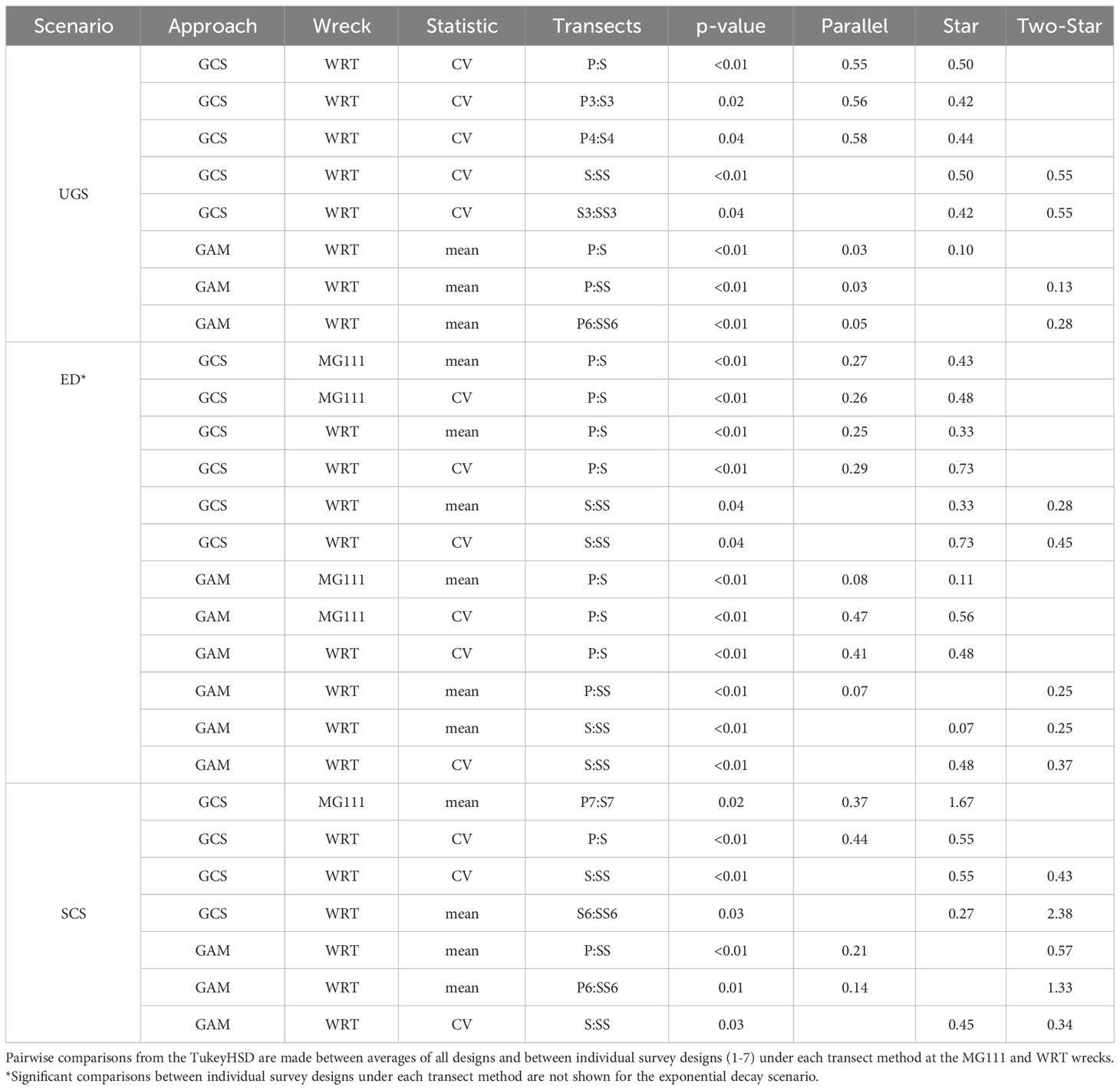
Table 4 Significant results of the two-way ANOVAs in the unconditional Gaussian, exponential decay, and stochastic conditional scenarios addressing H01: no difference in average RMAE of the mean or CV estimated by geostatistical conditional simulations and generalized additive models among parallel, star, and two-star transect methods.
Alterations of survey design were most influential to the model-based estimation of sA within the ED scenario, as all null hypotheses tested by the two-way ANOVA (H01:5) were rejected under this scenario (Tables 4–7). In this scenario, parallel transects were significantly less biased than star transects at MG111 for mean and variability estimated by both modeling designs (Table 4). Star transects also generated the largest error in mean and CV estimated at WRT by the GCS approach. When using the GAM approach, only precision in the variability of sA was lowest for star transects at WRT. Precision in mean sA was lowest for two-star transects under this approach.
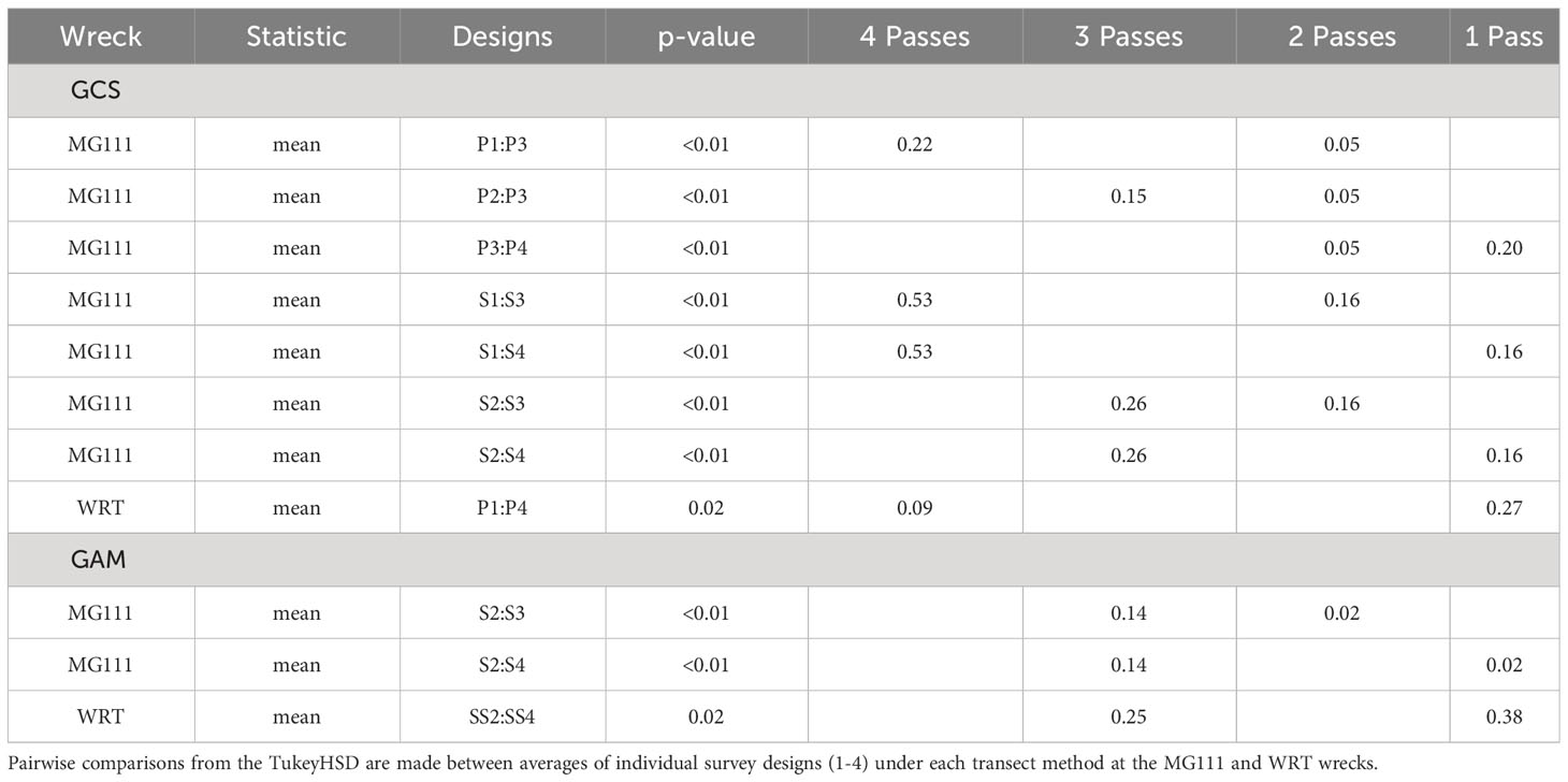
Table 5 Significant results of the two-way ANOVA in the exponential decay scenario addressing H02: average RMAE of the mean or CV estimated by geostatistical conditional simulations and generalized additive models is not influenced by the number of transects (1-4) which pass over the feature of interest.
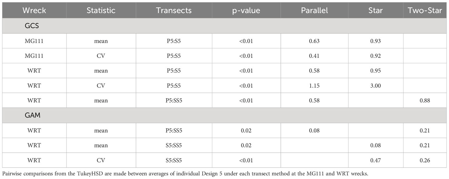
Table 6 Significant results of the two-way ANOVA in the exponential decay scenario addressing H03: no difference in average RMAE of the mean or CV estimated by geostatistical conditional simulations and generalized additive models among transect methods when no transects pass over the feature of interest.
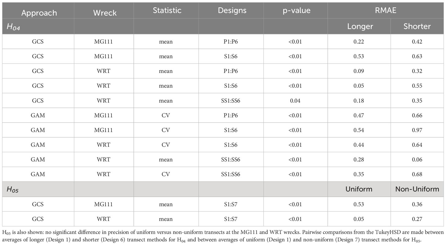
Table 7 Significant results of the two-way ANOVA in the exponential decay scenario addressing H04: transect length has no influence on the average RMAE of the mean or CV estimated by geostatistical conditional simulations and generalized additive models.
The null hypothesis of no difference in estimation error of mean sA among the number of transects that pass over the feature of interest (H02) was rejected at the single structure reef under both GCS and GAM (Table 5). Reducing the number of transects which pass over the structure resulted in an increase in precision for both the parallel and star transects at MG111 using the GCS approach. This trend was also significant in the GAM approach, but only for the star transect method. The number of transects passing over structures was less influential in the presence of a field of structures, where the only significant differences in precision were found between one pass and four or three passes for the parallel transects in the GCS approach and two-star transects in the GAM approach, respectively. We found no evidence that variability in sA is significantly affected by the number of transects passing over the habitat feature of interest, regardless of the number of features present.
In the case where passing over the feature of interest is not possible, the null hypothesis that the transect method does not influence mean or variability of sA (H03) predicted by GCS was rejected (Table 6). Parallel transects outperformed both star and two-star designs, irrespective of the number of structures present at the reef. At WRT, the two-star design generated less bias than the single star method in prediction of the mean. When using the GAM approach, error in the means predicted from the parallel and star designs were equal, and both were significantly less than the error predicted from the two-star design. However, error in the variability predicted from the star design was larger than the two-star design in this case.
Transect length (H04) had significant impacts on the mean and variability of sA predicted by both modeling approaches (Table 7). Under the GCS approach, precision in mean sA decreased with transect length for all transect methods at both wrecks. Under the GAM approach, precision in the CV of sA was affected more than the mean, although the mean sA at WRT had significantly larger bias from shorter transects in two-star surveys. Variability was better estimated by longer transects in all survey methods at the two wrecks when using GAM, except for the parallel method at WRT (p-value=0.09). Transect uniformity (H05) was the least impactful survey design alteration on precision of sA, and was only significant in the prediction of mean sA by GCS (Table 7). The results of this comparison suggest that when one structure is present, non-uniform transects produce less bias than uniform transects. When multiple structures are present, however, GCS results suggest that uniform transects produce less bias.
4 Discussion
4.1 Unconditional Gaussian scenario
In the UGS scenario, fish aggregations are small and randomly dispersed around the fixed point of interest (the shipwrecks in this study). This scenario may be representative of fish aggregations at expansive and structurally complex habitat features, such as natural reefs or fields of closely-placed artificial structures. These fish aggregations are weakly stationary, and were constructed in this case with an isotropic covariance structure (Figure 7). Of the three scenarios, the geostatistical modeling approach performed best in estimating the mean of fish aggregations simulated with these patchy and randomly dispersed distributions, as this scenario met the assumptions of stationarity and isotropy best (Table 1).
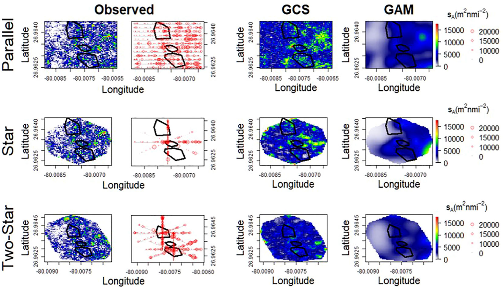
Figure 7 Simulated (left) sA interpolated by geostatistical conditional simulations and generalized additive models (right) in the unconditional Gaussian simulation scenario at WRT. Bubble plots (red circles with radii proportional to sA) show observations sampled by the ideal survey design (Design 1). Black polygons indicate the locations of the Esso Bonaire, Miss Jenny, and Zion Train shipwrecks.
The relative arrangement of transects when surveying such populations is arbitrary, unless large-scale trends are present in the distribution of fish. Three simulations at WRT exhibited a latitudinal gradient in the concentration of fish towards the edge of the survey area (offset from the three shipwrecks around which designs were centered). The distribution of fish at these simulations was non-stationary and anisotropic, and both properties were intensified for the sampled distribution in the application of star and two-star transects in comparison to parallel transects. The parallel transect method produced the most precise estimates of mean aggregation size even when using the GAM approach. Similar simulations of scallop populations have previously illustrated that geostatistical models produce more bias in comparison to non-geostatistical approaches (including GAMs) in the presence of large-scale spatial trends when sampling with parallel transects (Chang et al., 2017). Our results indicate that GAMs are also at least partially influenced by non-stationarity and anisotropy, and that the associated error is minimized in parallel transect designs compared to star transects.
4.2 Exponential decay scenario
The influence of disparities in stationarity and isotropy on precision of estimated fish quantities surveyed by different transect methods was best exemplified in the ED scenario (Figure 8). This scenario represents aggregations centered above an established location, such as a seamount or fish aggregating device (FAD). Density is highest in the center of the aggregation and decays exponentially with increasing distance in every direction. Samples of such aggregations only exhibit isotropy if the transects do not extend beyond the densest part of the aggregations (represented by survey Design 6 in the current study). For all transect methods in this case, variance in the sampled data distribution was low and the geostatistical model was more precise in measuring variability than GAMs, although error in both models was higher than when transects extended beyond the aggregation (Table 7).
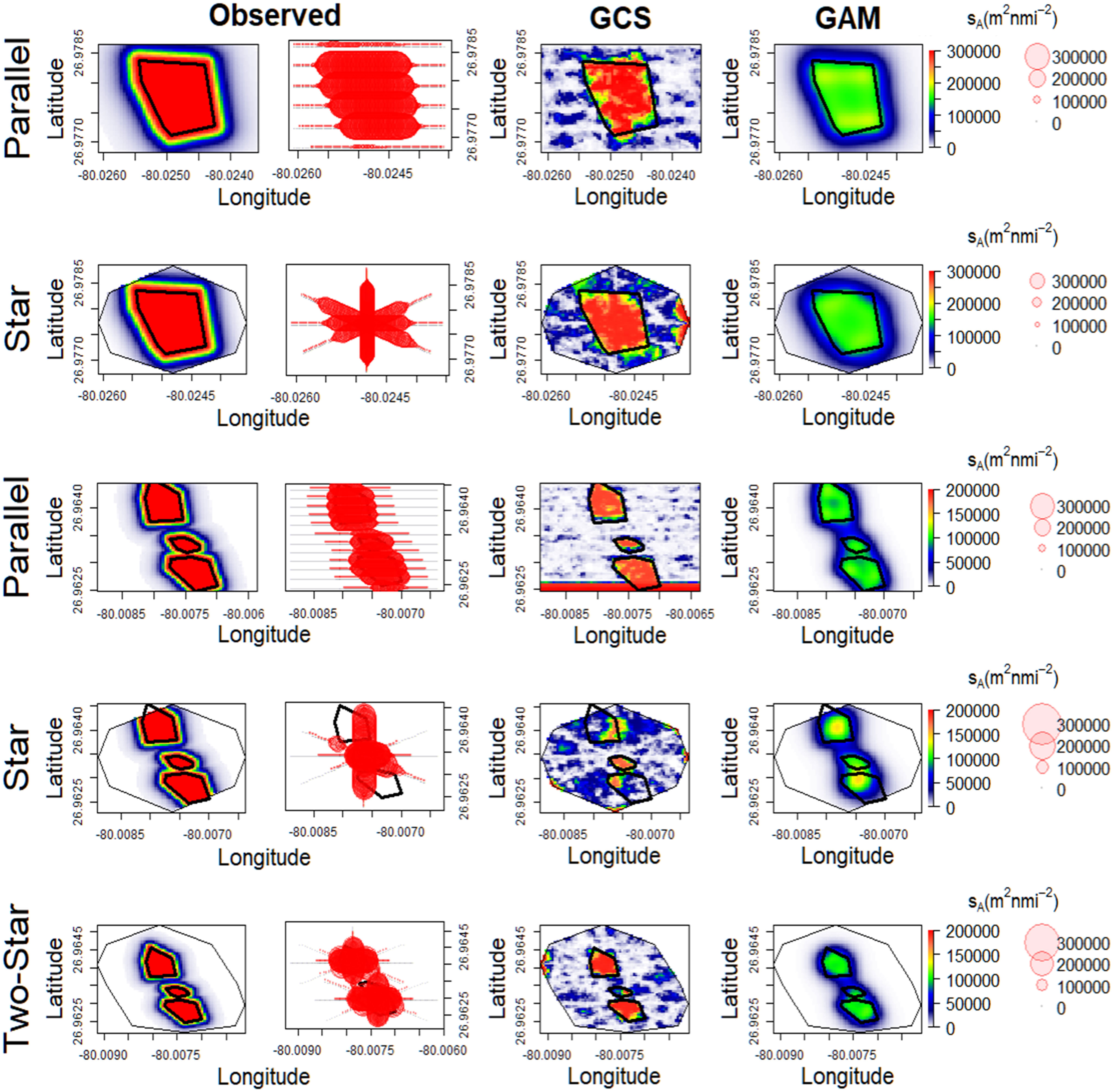
Figure 8 Simulated (left) sA interpolated by geostatistical conditional simulations and generalized additive models (right) in the exponential decay scenario at MG111 (top two rows) and WRT (bottom three rows). Bubble plots show sA observations sampled by the ideal survey design in each transect method (Design 1). Black polygons indicate the locations of each shipwreck.
Unlike the UGS and SCS scenarios, selection of transect starting points has a significant effect on bias in this scenario for aggregations fixed to a single point (Table 5). As long as at least one transect passes over the point of interest, increased sampling of the surrounding area where transects cross the edges of the aggregation can reduce bias in parallel and star designs when using GCS, and in star designs when using GAMs. Residual sampling autocorrelation is reduced in this case, which likely also contributes to improved precision. Doonan et al. (2003) simulated a similar scenario of orange roughy aggregations over seamounts and found that star surveys with transects offset from the fixed point of the seamount, but which still mostly pass over the aggregation, produced less-biased geostatistical estimates of biomass than stars with all transects intersecting at the center. Doray et al. (2008) utilized the star method to sample tuna aggregations around moored FADs and found that abundance estimation variance from universal kriging was reduced with increased number of transects over the FAD. Their results were purely based on the number of transects present in a traditional star survey design, and did not consider transects which do not cross the center of the aggregation, but rather provide higher sampling variance by increasing the number of samples around the edges of the aggregation. We propose that a more robust transect method for dense fish populations aggregated around a fixed location could include a random selection of transect starting points with a more even ratio of centered and offset transects driven in various directions. Further investigation is required to determine if such a “dropped sticks” survey design (similar to star Designs 3 or 4 at MG111 in this study) could minimize bias in the quantification of fish aggregations through reduced sampling autocorrelation and increased measure of variance when compared to parallel and star designs.
When considered as one population, fish aggregations fixed to multiple points (such as at WRT) are highly anisotropic under this scenario (Figure 8). There is no clear transect method which significantly increases precision in this case, although parallel designs produced less error in mean estimates (Table 4). In the situation where sampling over fish aggregations fixed to either single or multiple locations is not possible (Design 5 in this study), estimations will have large errors regardless of survey design. A prominent example of this situation in the nGOM are surveys of fishes at oil and gas platforms, where information is reliant on transects within close proximity to the structure but not within the structure frame which supports a large fish community. Our findings suggest that geostatistical estimations of mean and variability will be highly biased in this design, and are therefore not recommended (Table 6). GAM-based errors in the mean were much lower, but equal between parallel and star designs. Only bias from the two-star design at WRT was significantly greater in this case, indicating that there is no benefit from conducting separate surveys around each structure in a complex of multiple habitat features spaced within 100 m of each other.
4.3 Stochastic conditional scenario
The SCS scenario was simulated from acoustic data of live goliath grouper spawning aggregations at artificial reefs. This scenario is most representative of fish aggregations associated with established locations, but which exhibit fine-scale stochasticity around habitat features. Unlike the majority of UGS simulations considered here, these fish aggregations display significant spatial association to a structure without necessarily occurring directly over it. This scenario is most applicable to fish aggregations at artificial reefs and some seamounts. Unlike the ED scenario, the number, complexity, and exact location of aggregations is highly variable. For this reason, the occurrence of transects passing over fish aggregations is much less predictable than in either the UGS or ED scenarios (Figure 9).
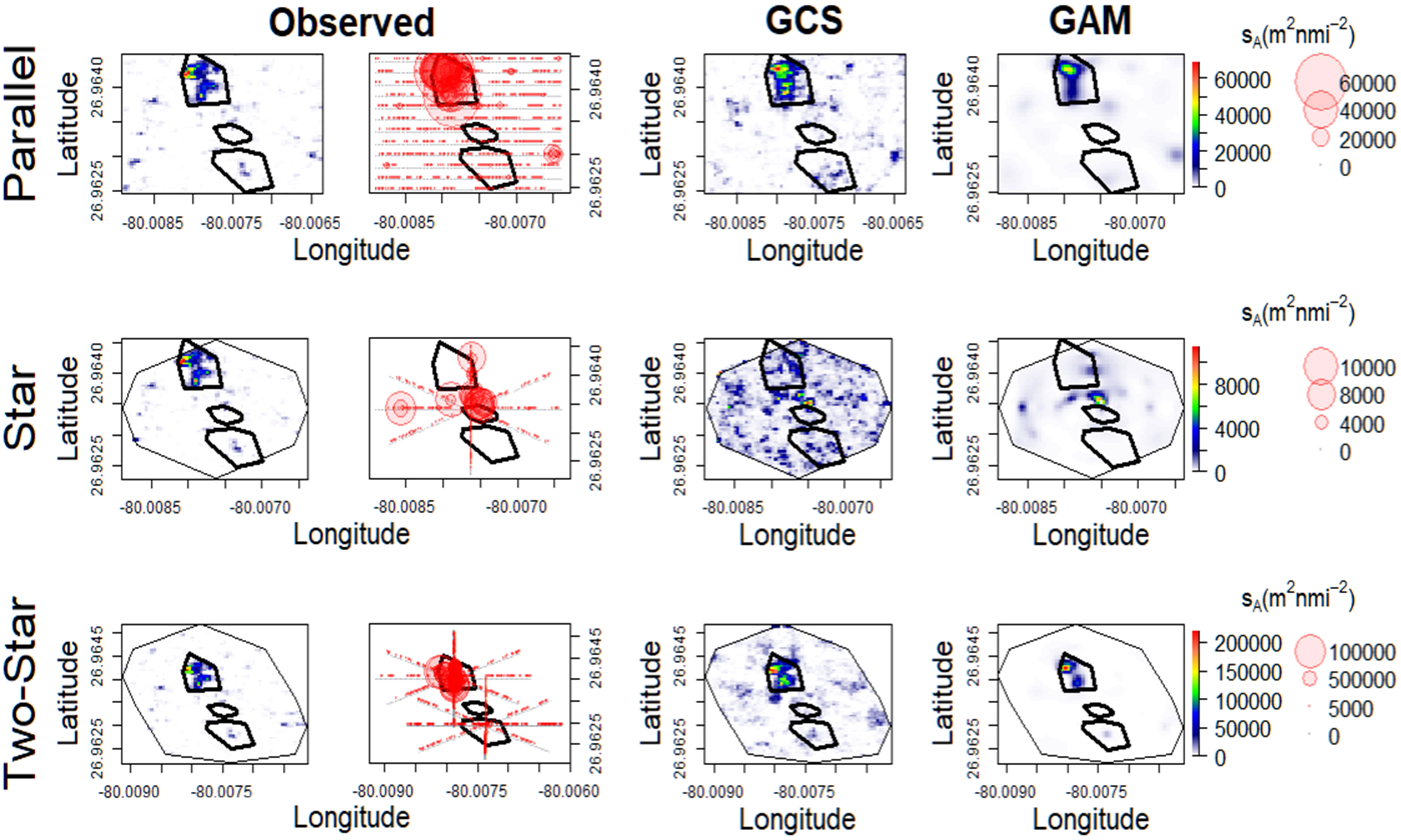
Figure 9 Simulated (left) sA interpolated by geostatistical conditional simulations and generalized additive models (right) in the stochastic conditional simulation scenario at WRT. Bubble plots show sA observations sampled by the ideal survey design in each transect method (Design 1). Black polygons indicate the locations of the three shipwrecks.
Star surveys of aggregations fixed to a single point reflect isotropy only if they intersect above the center of the aggregation (as observed by the star method at MG111 in the ED scenario, Figure 8), although this isotropy is highly reliant on the shape of the horizontal footprint of the aggregation. In their simulation of orange roughy aggregations around seamounts, Doonan et al. (2003) found that precision in kriging-based estimates of biomass was lower for star surveys which were not centered over the aggregations, and decreased further with increasing number and complexity of schools. Parallel transects were also considered in this study, although only for simulations where the centers of the aggregation and seamount overlapped (similar to the ED scenario in this study). The authors concluded that star designs outperform parallel designs for such aggregations only when the number of transects is low (<3), and that even when designs are centered over fixed-point aggregations there is no significant difference in the performance of either transect method in the presence of six or more transects. Our parallel transects outnumbered star transects at both the single structure reef (parallel=6, star=4) and the multi-structure reef complex (parallel=12, star=4, two-star=8). Mean estimates from parallel transects were only more precise than mean estimates from two-star transects at WRT and mean estimates from star designs in the non-uniform design (7) at MG111 (Table 4). However, parallel transects were more precise in estimation of variability, and are therefore recommended over star designs when the feature of interest and center of the fish aggregations are not necessarily coincident. The “dropped sticks” transect method described above could provide a compromise between sampling effort and estimation bias in this scenario, as we observed no significant influence on precision in designs where some transects in the star design did not cross the feature of interest (Designs 1-4). It should be noted that the parallel design is ultimately still preferable in this scenario, as stars and dropped sticks are both prone to over-sampling some locations and under-sampling others.
In all scenarios, there was little evidence to suggest that transect uniformity has a significant impact on precision. Transects performed by smaller vessels in non-ideal conditions (such as rough sea states, low boat visibility, impeding boat traffic, etc.) are equally as capable of providing robust quantitative estimates of fish aggregations as perfectly driven transects as long as trends in the underlying fish distribution are not impacted by the complicating conditions (as may be the case with current or moon phase for surveys conducted at night). Surveyors should not be deterred by the inability to drive perfect transects due to equipment limitations or poor weather conditions unless the quality of data collected is impacted (e.g. excessive dropout in split-beam echosounder data due to rough sea state). Variability in estimates was higher in parallel designs than in star designs under all scenarios except for the UGS scenario, where precision of variability in fish aggregations with large-scale trends offset from the point of interest was greater in the star design (but only using the GCS approach).
4.4 Conclusions
The evidence provided in this study supports the use of parallel survey designs over stars in most cases. In the few cases where error was equivalent between parallel and star designs, variability was still better estimated by the parallel design. In cross-habitat studies where fish aggregations may be represented by combinations of the three scenarios examined in this study, the star design generates more error in observations of fish aggregations similar to the UGS and ED scenarios, and is not recommended. In studies of fish aggregations at artificial reefs which mimic the patterns shown here by the SCS scenario, where there was no significant difference in error from either design, the lack of significant error reduction by performing one, two, three, or four passes over the habitat feature negates the preconceived benefit of maximizing passes over the feature. In instances where surveys are limited by time or cost of vessel operations, we recommend focusing effort on obtaining better measurements of variability as long as at least one pass is made over the habitat feature. As the residual spatial autocorrelation after modeling approaches have been implemented is still higher in star designs than in parallel designs and variability is better measured in the parallel design, we still recommend parallel designs over stars in this case.
We support the conclusion drawn from previous research of aggregated populations that GAMs are more robust than geostatistical approaches in the presence of both fine- and large-scale spatial trends which often result in non-stationary and anisotropic data (e.g. Yu et al., 2013; Chang et al., 2017). We add that these properties still have a strong influence on the precision of GAMs, but that precision can be improved with transect designs given some basic knowledge of how fish are aggregated around a point of interest. The survey designs and model approaches presented here will inform fisheries-independent sampling of the least-biased transect methods for quantifying fish aggregations when their underlying distribution is well-documented or understood, and that they will maximize the efficiency of adaptive sampling based on initial data when they are not.
Data availability statement
Most data was simulated. Acoustic dataset has not yet been published. Requests to access these datasets should be directed to BB,bbind002@fiu.edu.
Author contributions
AW, KB, and PS contributed to the conception and design of the study. KB and BB were awarded funding for data collection, which was conducted by BB, AW, and KB. Data processing was performed by BB. AW completed statistical analysis with guidance from PS. AW wrote the first draft of the manuscript. All authors contributed to the article and approved the submitted version.
Funding
Funding for the acoustic data collection was provided by NOAA MARFIN awarded to James Locascio and KB (NA15NMF4330152). This material is based upon work supported by the National Science Foundation under Grant No. HRD-1547798 and Grant No.HRD-2111661. These NSF Grants were awarded to Florida International University as part of the Centers of Research Excellence in Science and Technology (CREST) Program.
Acknowledgments
We greatly appreciate the assistance of Nicholas Tucker, Savannah LaBua, Olivia Odum, and Daniel Correa in conducting fieldwork for this study. This is contribution #1607 from the Coastlines and Oceans Division of the Institute of Environment at Florida International University.
Conflict of interest
The authors declare that the research was conducted in the absence of any commercial or financial relationships that could be construed as a potential conflict of interest.
Publisher's note
All claims expressed in this article are solely those of the authors and do not necessarily represent those of their affiliated organizations, or those of the publisher, the editors and the reviewers. Any product that may be evaluated in this article, or claim that may be made by its manufacturer, is not guaranteed or endorsed by the publisher.
References
Bates D. M., Watts D. G. (1988). Nonlinear Regression Analysis and Its Applications (New York, NY: Wiley).
Binder B. (2022). The patterns of occurrence, management, and behavioral ecology of fish spawning aggregations in southeast Florida (Miami, FL: Doctoral dissertation, Florida International University).
Boswell K. M., Wells R. J. D., Cowan J. H., Wilson C. A. (2010). Biomass, density and size distributions of fishes associated with a large-scale artificial reef complex in the Gulf of Mexico. Bull. Mar. Sci. 86 (4), 879–889. doi: 10.5343/bms.2010.1026
Chang J. H., Shank B. V., Hart D. R. (2017). A comparison of methods to estimate abundance and biomass from belt transect surveys. Limnol. Oceanogr.: Methods 15 (5), 480–494. doi: 10.1002/lom3.10174
Cressie N. (1993). Statistics for Spatial Data: Wiley Series in Probability and Statistics (New York, NY: John Wiley and Sons).
Demer D. A., Berger L., Bernasconi M., Bethke E., Boswell K., Chu D., et al. (2015). Calibration of acoustic instruments. ICES Cooperative Res. Rep. 326, 133. doi: 10.25607/OBP-185
Doonan I. J., Bull B., Coombs R. F. (2003). Star acoustic surveys of localized fish aggregations. ICES J. Mar. Sci. 60 (1), 132–146. doi: 10.1006/jmsc.2002.1331
Doray M., Petitgas P., Josse E.. (2008). A geostatistical method for assessing biomass of tuna aggregations around moored fish aggregating devices with star acoustic surveys. Can. J. Fish. Aquat. Sci. 65, 1193–1205. doi: 10.1139/F08-050s
Dunn P., Smyth G. (2005). Series evaluation of Tweedie exponential dispersion models. Stat Comput. 15, 267–280. doi: 10.1007/s11222-005-4070-y
Gregoire T. G. (1998). Design-based and model-based inference in survey sampling: appreciating the difference. Can. J. For. Res. 28, 1429–1447. doi: 10.1139/x98-166
Gunderson D. R. (1993). Surveys of Fisheries Resources (New York, NY: John Wiley and Sons, Inc.), 248.
Hieu N. T., Brochier T., Tri N. H., Auger P., Brehmer P. (2014). Effect of small versus large clusters of fish school on the yield of a purse-seine small pelagic fishery including a marine protected area. Acta Biotheoretica 62, 339–353. doi: 10.1007/s10441-014-9220-1
Jolly G. M., Hampton I. (1990). A stratified random transect design for acoustic surveys of fish stocks. Can. J. Fish. Aquat. Sci. 47, 1282–1291. doi: 10.1139/f90-147
Kang M., Nakamura T., Hamano A. (2011). A methodology for acoustic and geospatial analysis of diverse artificial-reef datasets. ICES J. Mar. Sci. 68 (10), 2210–2221. doi: 10.1093/icesjms/fsr141
Koenig C. C., Bueno L. S., Coleman F. C., Cusick J. A., Ellis R. D., Kingon K., et al. (2017). Diel, lunar, and seasonal spawning patterns of the Atlantic goliath grouper, Epinephelus itajara, off Florida, United States. Bull. Mar. Sci. 93 (2), 391–406. doi: 10.5343/bms.2016.1013
MacLennan D. N., Fernandes P. G., Dalen J. (2002). A consistent approach to definitions and symbols in fisheries acoustics. J. Mar. Sci. 59, 365–369. doi: 10.1006/jmsc.2001.1158
MINES ParisTech/ARMINES. (2022). RGeostats: The Geostatistical R Package. Available at: http://cg.ensmp.fr/rgeostats.
Neyman J. (1934). On the two different aspects of the representation method - the method of stratified sampling and the method of selection. J. R. Statist. Soc 97, 558–606. doi: 10.2307/2342192
R Core Team. (2022). R: A language and environment for statistical computing (Vienna, Austria: R Foundation for Statistical Computing). Available at: https//www.R-project.org/.
Rivoirard J., Simmonds J., Foote K. G., Fernandes P., Bez N. (2000). Geostatistics for Estimating Fish Abundance (Oxford, UK: Blackwell Science, Oxford), 206.
Scheaffer R. L., Mendenhall W. III, Ott R. L., Gerow K. G. (2012). Elementary Survey Sampling. 7th edn (Boston, MA: Cengage Learning).
Taylor J. C., Eggleston D. B., Rand P. S. (2006). “Nassau grouper (Epinephelus striatus) spawning aggregations: hydroacoustic surveys and geostatistical analysis,” in In Emerging Technologies for Reef Fisheries Research and Management. Ed. Taylor J. C. (Tortola, British Virgin Islands: NOAA Professional Paper), 18–25.
White A. L., Patterson W. F. III, Boswell K. M. (2022). Distribution of acoustic backscatter associated with natural and artificial reefs in the Northeastern Gulf of Mexico. Fisheries Res. 248, 106199. doi: 10.1016/j.fishres.2021.106199
Woillez M., Rivoirard J., Fernandes P. G. (2009). Evaluating the uncertainty of abundance estimates from acoustic surveys using geostatistical simulations. ICES J. Mar. Sci. 66, 1377–1383. doi: 10.1093/icesjms/fsp137
Woillez M., Walline P. D., Ianelli J. N., Dorn M. W., Wilson C. D., Punt A. E. (2016). Evaluating total uncertainty for biomass-and abundance-at-age estimates from eastern Bering Sea walleye pollock acoustic-trawl surveys. ICES J. Mar. Sci. 73 (9), 2208–2226. doi: 10.1093/icesjms/fsw054
Wood S. N. (2003). Thin-plate regression splines. J. R. Stat. Soc. B 65 (1), 95–114. doi: 10.1111/1467-9868.00374
Wood S. N. (2017). Generalized Additive Models: An Introduction with R. 2nd ed. (Boca Raton, FL: Chapman and Hall/CRC).
Keywords: fish aggregations, active acoustics, survey design, star surveys, model-based inference, generalized additive models, geostatistics, fisheries-independent surveys
Citation: White AL, Sullivan PJ, Binder BM and Boswell KM (2023) An evaluation of survey designs and model-based inferences of fish aggregations using active acoustics. Front. Mar. Sci. 10:1176696. doi: 10.3389/fmars.2023.1176696
Received: 28 February 2023; Accepted: 16 August 2023;
Published: 04 September 2023.
Edited by:
Fabio Campanella, Centre for Environment, Fisheries and Aquaculture Science (CEFAS), United KingdomReviewed by:
Jorge Paramo, University of Magdalena, ColombiaSerdar Sakinan, Wageningen Marine Research IJmuiden, Netherlands
Copyright © 2023 White, Sullivan, Binder and Boswell. This is an open-access article distributed under the terms of the Creative Commons Attribution License (CC BY). The use, distribution or reproduction in other forums is permitted, provided the original author(s) and the copyright owner(s) are credited and that the original publication in this journal is cited, in accordance with accepted academic practice. No use, distribution or reproduction is permitted which does not comply with these terms.
*Correspondence: Allison L. White, awhit100@fiu.edu