Evaporation induced convection enhances mixing in the upper ocean

The upper ocean surface layer is directly affected by the air-sea fluxes. The diurnal variations in these fluxes also cause the upper ocean mixed layer turbulence and mixing to diurnally vary. The underlying thermohaline structure also varies accordingly throughout the day. Here we use large-eddy simulation to quantify the role of surface evaporation in modulating the diurnal mixed layer turbulence and mixing in the presence of wind forcing. During daytime, the upper ocean boundary layer becomes thermally stratified, and a salinity inversion layer is formed in the upper 10m, leading to double diffusive salt-fingering instability. During nighttime, the mixed layer undergoes convective deepening due to surface buoyancy loss redfrom both surface cooling and evaporation. We find that salinity makes a major contribution to the convective instability during both transitions between day and night. Overall surface evaporation increases the mixed layer depth and irreversible mixing through convection, both during nighttime and daytime, and leads to better prediction of the dynamical variables as sea surface salinity (SSS) and sea surface temperature (SST). Our findings can help improve the ocean parameterizations to improve the forecasts on a diurnal timescale.

1 Introduction

The ocean mixed layer (OML) is highly turbulent with nearly uniform vertical distribution of temperature, salinity and density. The mixed layer mediates the exchange of mass, momentum, heat and freshwater between the atmosphere and the ocean. The time-varying surface fluxes and the depth of the OML are both important determinants of sea surface temperature (SST), sea surface salinity (SSS) and ocean heat content. Thus it is imperative to understand the mixed layer dynamics, turbulence and the associated irreversible mixing under various external conditions in a rapidly changing climate.

The fluxes of momentum, heat and freshwater at the ocean surface vary on all time scales, the diurnal scale being one of the most prominent. The net surface heat flux is the sum of shortwave radiation, net longwave radiation, latent heat flux and sensible heat flux. Shortwave (solar) radiation incident at the ocean surface, as well as net surface heat flux, have well-marked diurnal variability, tending to heat the ocean in the daytime and cooling the ocean at night. The other components of heat flux also have diurnal variations. For example, latent heat flux varies due to diurnal changes in surface winds (Wallace and Hartranft, 1969; Stull, 1988; de Szoeke et al., 2021).

The ocean responds to the boundary forcing and changes some of the key variables that define the ocean state. The solar radiation is absorbed by the water column during daytime, in a volumetric sense (Paulson and Simpson, 1977), while the combined effect of non solar components cool the air-sea interface at almost all the times, also called as the cool skin effect (Fairall et al., 1996). As a result, the OML generally deepens during the nighttime cooling, when this convective turbulence tends to dominate, while the near surface generally gets stratified in the daytime, leaving behind a remnant mixed layer (Brainerd and Gregg, 1993). The SST also varies during this time, due to this net heating during the daytime and cooling in nighttime. These processes are interdependent as the daytime’s stratification is dictated by how deep the OML was during nighttime, and consequently the nighttime deepening depends on the strength of the daytime stratification. Wind shear transfers momentum flux into the ocean. Under weak winds, the turbulent mixing is suppressed (Hughes et al., 2020b) leading to strong diurnal SST variations (Flament et al., 1994; Soloviev and Lukas, 1997; Sui et al., 1997) and vice versa under strong winds (Yan et al., 2021). Evaporation happens at all times in the ocean, increasing the sea surface salinity (SSS) but precipitation occurs only during wet spells. The combined effect of this saltier and cooler skin makes it always statically unstable (Saunders, 1967; Yu, 2010). The upper ocean thus experiences diurnal variations in both momentum and buoyancy (heat) fluxes and undergoes a diurnal cycle of turbulence and mixing (Lombardo and Gregg, 1989; Brainerd and Gregg, 1993; Moulin et al., 2018).

Several previous studies have focussed on the response of the upper ocean to diurnally varying surface forcing using observations and model experiments. Lombardo and Gregg (1989) took microstructure measurements at 34°N, made during the PATCHEX experiment (1986) and gave a similarity scaling for the turbulence occurring during nighttime convection. The kinetic energy dissipation was normalized by the sum of scalings obtained from wind stress driven and convectively driven turbulence. Using the same dataset, the restratification processes and the daily cycle of turbulence within the OML were analyzed (Brainerd and Gregg, 1993). Price et al. (1986) used field observations from 30.9°N to analyze the diurnal response and to further develop the widely used one-dimensional Price-Weller-Pinkel model (PWP). This is a slab model, integrating and balancing quantities over the entire OML. In the equatorial Pacific, a linear stability analysis was used to show that the enhanced near-surface shear that forms in the daytime, descends in the evening, leaving the nighttime mixing layer above it (Smyth et al., 2013). This layer merged with the deeper Equatorial Undercurrent, triggering deep cycle turbulence. This study was supplemented with ship-based measurements of velocity, stratification and turbulent dissipation (Moum et al., 2009). Large-eddy simulations using temperature as a single scalar were conducted (Pham et al., 2013; Pham et al., 2017) to study the dynamic processes leading to deep cycle turbulence and its seasonality. In the equatorial Atlantic, using PIRATA mooring data, Wenegrat and McPhaden (2015) explored diurnal stratification, shear and SST. They also hinted at the possibility of deep cycle turbulence, owing to the presence of marginal instability between the OML and the thermocline. In the Indian Ocean, the surface diurnal warm layer was studied during the DYNAMO experiment (Matthews et al., 2014). From the DYNAMO measurements, de Szoeke et al. (2021) demonstrated that convective turbulence in the atmosphere is caused by diurnal ocean warming. The Bay of Bengal is known for a shallow salinity -stratified layer due to copious freshwater input from rivers and rainfall during summer monsoon season. Idealized turbulence-resolving simulations for the Bay of Bengal were conducted to explore the diurnal OML turbulence by Sarkar and Pham (2019), who concluded that the mixed layer salinity changed solely due to the entrainment of saltier subsurface water. The effects of haline forcing were studied by Drushka et al. (2016; 2014), who examined the diurnal salinity cycle in the tropics, and the dynamics of the upper ocean after rain events using the General Ocean Turbulence Model (GOTM). The diurnal amplitude of salinity anomalies, with major contributions from diurnal entrainment and precipitation, were found to be around ∼ 0.005 PSU. Yu (2010) tried to study the effect of evaporation on the salty skin. However to the best of our knowledge, none of the above mentioned studies focused on the role of evaporative fluxes and resulting changes in SSS in modifying and quantifying the irreversible turbulent mixing in the OML.

We conduct large-eddy simulations of the ocean, representative of the Bay of Bengal, using both temperature and salinity as active scalars, with diurnally varying forcing to quantify the upper ocean turbulence and mixing. The results provide new insights into the spatio-temporal character of diurnal turbulence and mixing. We show that the evaporation can play a major role on diurnal timescales for controlling the SSS and hence enhancing the mixing in the surface layer. We also show the existence of a salinity inversion layer and the presence of salt-fingering instability, during daytime, for the case of weak winds, due to evaporation.

2 Methodology

To perform the convection resolving simulations, we take a cuboidal domain at centered around the Bay of Bengal mooring (Weller et al., 2016) at 18°N, 89.5°E of dimensions 100m × 100m × 250m. Periodic boundary conditions are imposed in the horizontal directions so as to remove the effect of any lateral density gradients. The domain is bounded at the top by a flat air-sea interface, where we prescribe the boundary conditions of momentum, heat and evaporative haline (salt) fluxes. These boundary conditions are based on smoothed air-sea fluxes (Figure 1A) taken from the mooring observations during wintertime in the Bay (Weller et al., 2019). The evaporation rate $E$ (m/s) is calculated from the latent heat flux $Q_L$ as:

FIGURE 1

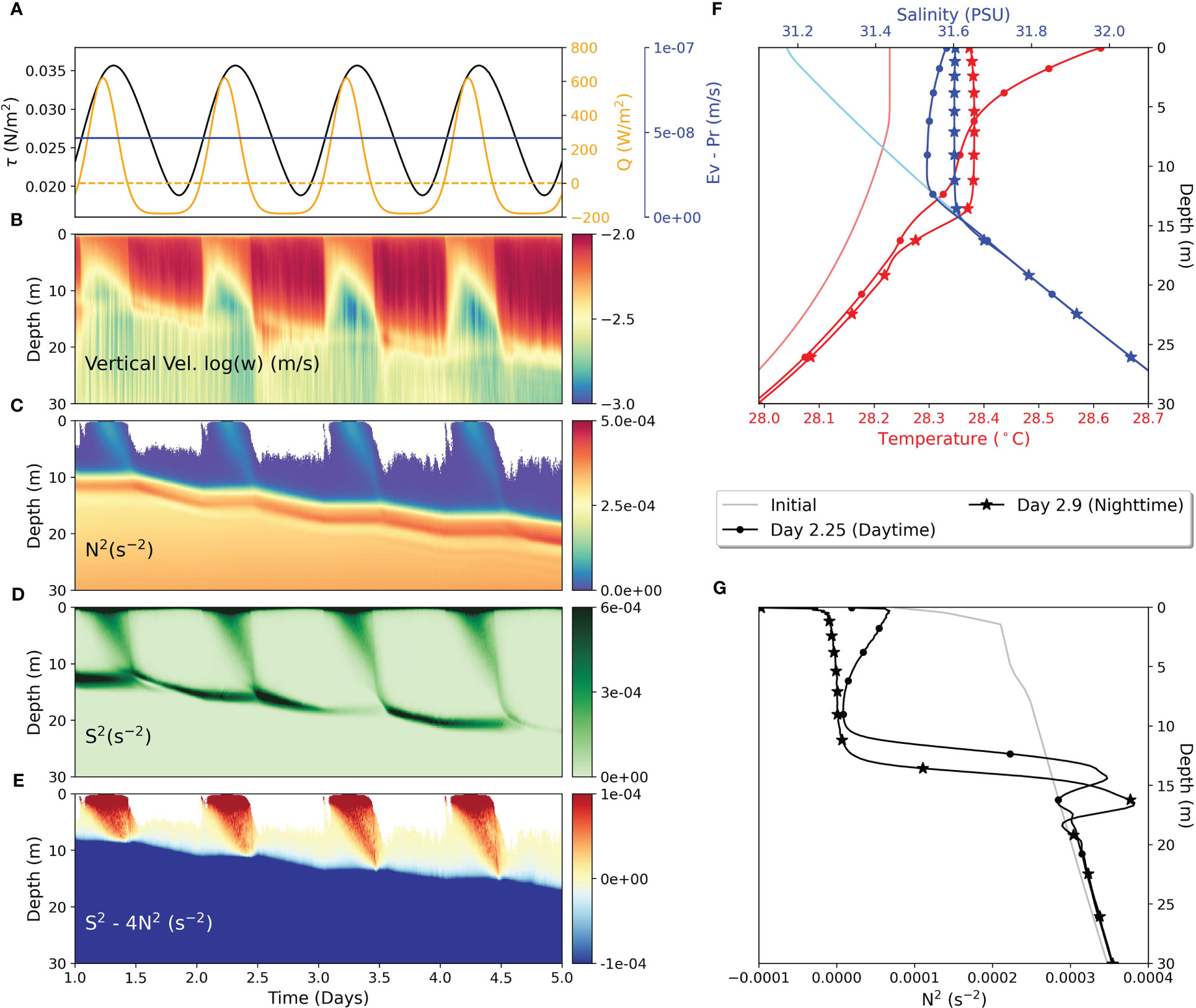
Figure 1 (Left) Upper ocean response to diurnal forcing. (A) Surface boundary conditions of net heat flux Q (W/m²) (orange), wind stress magnitude τ (N/m²) (black) and evaporation minus precipitation E-P (m/s) (blue). (B) Horizontally averaged root mean squared fluctuating vertical velocity w (m/s). (C) Brunt Vaisala Frequency squared $N^2$ (s ${}^{-2}$ ), where white patches indicate $N^2<0$. (D) Shear squared $S^2$ (s ${}^{-2}$). (E) Reduced shear or Modified Richardson number $S^2$ - 4 $N^2$ (s ${}^{-2}$). (F, G) Initial profiles of T, S and $N^2$ (solid), at day 2.25 (dotted) and day 2.9 (star marked).

$\begin{array}{ll}E=\frac{Q_L}{{\rho }_0{L}_v}& (1)\end{array}$

where ${\rho }_0$ is the reference density and. is the latent heat of vaporization. We also include the effects of shortwave penetration by putting it as a source term in the governing equations. Here we have also put diurnally oscillating wind stress to give unsteadiness to the system. We also add a sponge layer of height 50m, extending up to 200m so as to damp any reflections coming from the bottom boundary thus mimicking open ocean conditions. Note that this study does not include the effects of precipitation, as it has been well documented in an earlier study (Drushka et al., 2016).

Large-eddy simulations are used to evaluate the velocity and scalar fields (temperature and salinity) from the incompressible, non-hydrostatic Navier-Stokes equation, with Boussinesq and f-plane approximation. Additional model details can be found in the Supplementary Document. We employ a linear equation of state for calculating the density field. The LES domain uses a grid of $N_x=N_y=128$ and $N_z=417$ which is uniform in both the $x$ and $y$ directions and stretched in the $z$ direction to achieve higher resolution near the top boundary in order to resolve the $\sim \mathcal{O}(1mm)$ thick laminar diffusive layer. The required resolution criteria is discussed in Rosevear et al. (2021). Model runs are initialized with temperature and salinity profiles, fitted from the mooring observations prior to the event (Figures 1, S1). The water has a molecular viscosity of $\nu ={10}^{-5}$ m²/s, thermal diffusivity ${\kappa }_T=1.4\times {10}^{-6}$ m²/s and salt diffusivity ${\kappa }_S=1.2\times {10}^{-8}$ m²/s. Variable time stepping with a fixed Courant–Friedrichs–Lewy (CFL) number of 1.2 and typical time steps of the order $\mathcal{O}(1s)$ is used. To quantify the role of evaporation, two sets of simulations have been performed: a) complete forcing with momentum, heat and haline fluxes, and b) forcing with momentum and heat fluxes only. Note that we also performed simulations with constant wind stress, but it didn’t have much effect on the resulting dynamics (Figure S4). All the further analysis has been done from the second diurnal cycle onward, as the model spin-up time was about one day.

3 Results

3.1 Overview of diurnal turbulence

The diurnal nature of the surface fluxes cause the upper ocean to cyclically stir and restratify. During the nighttime, the negative net heat flux cools the surface of the ocean (Figure 1A), and results in unstable stratification (Figures 1C, G) and convective deepening of the OML. Convective plumes penetrate into the subsurface depths reaching the diurnal pycnocline, as can be seen from the horizontally averaged root mean squared fluctuating vertical velocity, which varies over an order of magnitude, and the Brunt- Väisäla frequency squared (N2)

$\begin{array}{ll}{N}^2=\frac{-g}{{\rho }_0}\frac{d\langle \rho \rangle }{dz}& (2)\end{array}$

where $g$ is the acceleration due to gravity, ${\rho }_0$ is the reference density and $\langle \rho \rangle$ is the total horizontally averaged density, (Figures 1B, C) which peaks at around 4 $\times {10}^{-4}$ s ${}^{-2}$ within the pycnocline (Figure 1G). As the daytime begins and the shortwave is absorbed by up the ocean bulk, most of the turbulence is suppressed and thermal stratification begins to build and the OML shallows (Figures 1F, G). The increased stratification traps horizontal momentum within a very thin layer, called the diurnal warm layer, enhancing the near-surface shear. The squared shear $S^2$(Figure 1D) is calculated as:

$\begin{array}{ll}{S}^2={\left(\frac{d\langle u\rangle }{dz}\right)}^2+{\left(\frac{d\langle v\rangle }{dz}\right)}^2& (3)\end{array}$

where $\langle u\rangle$ and $\langle v\rangle$ are the plane averaged zonal and meridional velocities respectively. This shear layer descends towards the pycnocline, as the net heat flux begins to decrease after reaching its peak value. Note that, at all times the oscillating surface wind stress also continues to produce shear turbulence, but it is enhanced near the surface during daytime and near the pycnocline during the nighttime. This phenomena has also been documented in previous studies (Moulin et al., 2018; Hughes et al., 2020a). Figure 1E shows the reduced squared shear $S^2$ - 4$N^2$, where positive values indicate that the water column is unstable to KH-like shear instability. The competition between this diurnal jet and stratification makes the near-surface unstable to shear instabilities. In addition, we also see the subsurface depths getting unstable as this shear layer descends (Moulin et al., 2018; Wijesekera et al., 2020). Evaporation leads to a persistent unstable gradient of near surface salinity (Figure 1F), which is present even during daytime. This enhances the convective instability during nighttime and also compensates for the increase in the overall stratification during daytime due to thermal heating alone. This also causes enhanced mixing, especially during daytime, as will be discussed further.

3.2 Salt-fingering instability in the diurnal mixed layer

Surface evaporation tends to increase the SSS (Asher et al., 2014; Drushka et al., 2014; Boutin et al., 2016). The accumulation of heat and excess salinity in the top layer over colder and fresher deeper waters are the conditions favorable for double diffusive salt-fingering instability (Soloviev and Lukas, 1997). This is quantified using the density ratio $R$ and Turner angle $Tu$ defined as:

$\begin{array}{ll}R=\frac{\alpha T_z}{\beta S_z}=-\tan (Tu+{45}^{\circ })& (4)\end{array}$

where $\alpha$ and $\beta$ are the thermal expansion and haline contraction coefficients, and $T_z$ and $S_z$ denote the plane averaged vertical temperature and salinity gradients (Ruddick, 1983). For warm/salty waters over cold/fresh, ${}^{-45°<Tu<45°}$, indicating salt-fingering (SF) instability is likely, whereas $-{45}^{\circ }<Tu<{90}^{\circ }$ indicates absolute stability. However $Tu<-{90}^{\circ }$ or $Tu>{90}^{\circ }$ denotes static instability ($N^2<0$). The former is caused due to the overwhelming effect of destabilizing thermal gradient and the latter vice versa. Figure 2B shows the temporal evolution of $Tu$ for two consecutive diurnal cycles. During the daytime, the entire water column down to the pycnocline is susceptible to salt-fingering instability. L424 This can also be verified from the T/S profiles in Figure 2D during daytime. Figure 2E shows the contribution of both scalar gradients to the overall stratification. They are defined as:

FIGURE 2

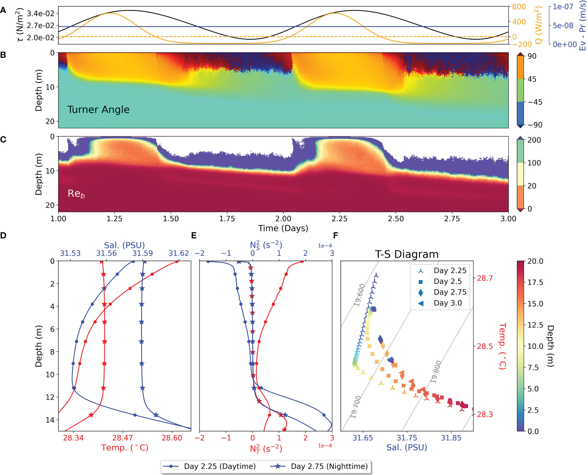
Figure 2 (A) Wind stress magnitude τ (N/m²) (black), net heat flux Q (W/m²) (orange) and evaporation minus precipitation E-P (m/s) (blue). (B) Turner angle $Tu$ from LES simulations. (C) Buoyancy Reynolds number $R{e}_b$ contour from LES simulations, where white patches indicate $N^2<0$. (D, E) Depthwise profiles of temperature T, salinity S and $N_T^2$, $N_S^2$ plotted at day 2.25 (dotted) and day 2.75 (star marked). (F) TS diagram plotted at day 2.25, 2.5, 2.75, 3.0 till 20m depth.

$\begin{array}{ll}{N}_T^2=g\alpha \frac{\langle \partial T\rangle }{\partial z}\text{\hspace{1em}\hspace{1em}and\hspace{1em}\hspace{1em}}{N}_S^2=-g\beta \frac{\langle \partial S\rangle }{\partial z}& (5)\end{array}$

The salinity gradient compensates the temperature gradient in the daytime, however keeping the overall stratification stable. When the surface heat flux changes sign from positive to negative, indicating a shift from daytime to nighttime, both the scalars contribute negatively to the stratification, causing convective static instability. This implies that both $N_T^2,N_S^2<0$. However, since the boundary condition of temperature changed from heating to cooling, it takes some time to adjust. Hence initially, even if both $N_T^2,N_S^2<0$, but $\left|N_T^2\right|<\left|N_S^2\right|$, making the contribution of salinity gradient the dominant effect in destabilizing the density gradient. This can also be seen through Turner angle, where the near surface values are more than 90° just as the heat flux changes sign from positive to negative. After some time however, the values of Turner angle become less than -90° indicating that surface cooling dominates the convective mixing. The convection almost homogenizes both the T/S profiles, leaving almost negligible gradient, except near the top, where the localized effects of both surface cooling and evaporation persist (Figures 2D, E). As soon as the shortwave begins however, even when the heat fluxis still negative, the turbulence begins to decrease due to the build up of thermal stratification and increased potential energy. At that instant, the convection switches back to being salinity dominated and the whole cycle repeats the next day.

To supplement the findings above, we also plot the buoyancy Reynolds number, calculated as:

$\begin{array}{ll}R{e}_b=\frac{ϵ}{\nu N^2}& (6)\end{array}$

where $ϵ$ is the turbulent kinetic dissipation (defined in the next section) and $N^2$ is the squared Brunt Vaisala frequency. This quantity can be interpreted as the ratio of Ozmidov to Kolmogorov length scales. For $R{e}_b<20$, there is weak buoyancy controlled turbulence, while for $R{e}_b>100$ the turbulence is energetic (Bouffard and Boegman, 2013). Previous studies have indicated that salt-fingering can enhance mixing for $R{e}_b<200$ (Nagai et al., 2015). Figure 2C shows that during daytime, $R{e}_b<200$ almost throughout the diurnal thermocline, which further supports that salt-fingering is the major contributor to turbulent mixing. The TS diagram (Figure 2F) provides another description of these dynamics. It has been plotted every 6 hours, for the whole of day 2 (after initialization). By day 2.25, when the neat heat flux is positive, in the top 7m or so the presence of warm and salty waters over cold and fresh waters and indication of salt-fingering can be seen here as well. Soon after nighttime begins (day 2.5), a small inversion can be seen in both the scalars due to the net surface destabilizing buoyancy flux. During peak night times, the profiles have been almost homogenized down to the pycnocline, which can be seen by both day 2.5 and 3. Note that the changes in these T/S properties only occur for depths less than about 15m, as the OML itself is about 13m. These changes in time have profound consequences on irreversible turbulent mixing, discussed in the next section.

3.3 Turbulence statistics and mixing

Figure 3 shows the evolution of horizontally averaged turbulence statistics from the ocean’s response. The small scale turbulent kinetic energy (Figure 3B) is defined as:

FIGURE 3

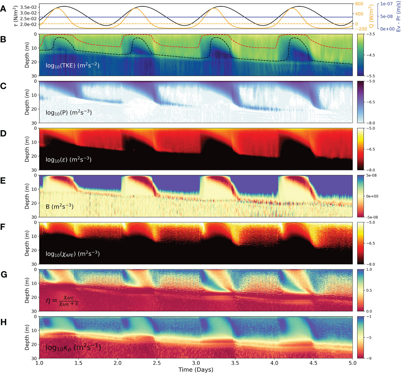
Figure 3 Turbulence and mixing statistics for the upper ocean. (A) Wind stress magnitude τ (N/m²) (black), net heat flux Q (W/m²) (orange) and evaporation minus precipitation E-P (m/s) (blue). (B) Turbulent Kinetic Energy (TKE) with the mixed layer depth for case with evaporation (black) and without evaporation (red). (C) Shear Production $P$ . (D) Total kinetic dissipation $ϵ$. (E) Turbulent Buoyancy Flux $B$. (F) Mixing ${\chi }_{APE}$ defined as the sink of APE. (G) Mixing efficiency $\eta$. (H) Diapycnal Diffusivity ${\kappa }_{\rho }$ calculated following (Osborn and Cox, 1972). Panels (B–D, F, H) show the logarithm of respective quantities.

$\begin{array}{ll}TKE=\frac{1}{2}\langle {\mathrm{ui}}_{{}^{\prime }}{\mathrm{ui}}_{{}^{\prime }}\rangle & (7)\end{array}$

where, $u_i{}^{\prime }$ , the fluctuating velocity, is calculated from the horizontally averaged mean field as $u_i{}^{\prime }=u_i-\langle u_i\rangle$ ($\langle .\rangle$ denotes horizonatlly averaged quantity). During nighttime, TKE is enhanced within the whole mixed layer due to convection, while it is restricted to the near-surface during daytime. The mixed layer depth (MLD) for both the test cases, calculated using a density threshold criteria of 0.01 kg/m³ is also plotted. It varies diurnally for both the cases, however the combined case has greater MLD than the case without evaporation. Using higher thresholds may cause MLD to not shallow much during daytime. A continued increase over time of MLD for the combined case, can be observed as the net surface buoyancy flux integrated over a day is non-zero (and positive) and the surface wind stress also continues to provide a source of mechanical turbulence all the time. There is some leakage of TKE below the mixed layer as well, which is likely due to the downward propagation of internal waves from the pycnocline. The shear production P (Figure 3C) shows the variability of mechanically generated turbulence, given by

$\begin{array}{ll}P=-\langle {\mathrm{ui}}_{{}^{\prime }}{\mathrm{uj}}_{{}^{\prime }}\rangle \frac{\partial \langle u_i\rangle }{\partial x_j}& (8)\end{array}$

The enhanced values near the surface are the direct result of the stress applied, while the descent of the shear layer causes shear instability and turbulence, as discussed before (Figure 1E). The subsurface enhancement of shear production within the pycnocline can be seen during nighttime, producing internal waves. The turbulent buoyancy flux.

$\begin{array}{ll}B=-\frac{g}{{\rho }_0}\langle {\rho }^{\prime }{w}^{\prime }\rangle & (9)\end{array}$

represents the conversion of energy from TKE to available potential energy (APE) and vice versa (Figure 3E). This includes contributions from both the scalars respectively. Positive values indicate APE being converted to TKE, through convection, while negative values show the energy spent in destroying stable stratification (conversion from TKE to APE). During nighttime, the turbulence is mostly convective in nature, while during the daytime, the shear-induced turbulence has to work against the stable stratification. The turbulent kinetic dissipation $ϵ$ is the sink of TKE, denoting how much energy is spent in overcoming the viscous stresses.

$\begin{array}{ll}ϵ=\nu \langle \frac{\partial {\mathrm{ui}}_{{}^{\text{'}}}}{\partial x_j}\frac{\partial {\mathrm{ui}}_{{}^{\text{'}}}}{\partial x_j}\rangle & (10)\end{array}$

As discussed before, depending on the time of the day, the turbulence could be either mechanical or convective in nature. The dissipation also follows this variability (Figure 3D). During the daytime, the values of $ϵ$ and $P$ are comparable near the surface and during descent of the shear layer. However, in the convective regime, the buoyancy flux tries to balance $ϵ$, throughout the mixed layer. This has also been reported in previous studies (Shay and Gregg, 1986; Lombardo and Gregg, 1989; Ivey and Imberger, 1991; 214 Imberger, 1985).

The irreversible mixing, defined as the sink of APE, is calculated following Gregg (2021) (Figure 3F).

$\begin{array}{ll}{\chi }_{APE}=\frac{g^2}{{\rho }_0^{2}N{*}^2}{\chi }_{\rho }& (11)\end{array}$

where ${\chi }_{\rho }$ is the rate of destruction of density variance or scalar dissipation.

$\begin{array}{ll}{\chi }_{\rho }=2{\kappa }_{\rho }⟨\frac{\partial {\rho }^{\prime }}{\partial x_i}\frac{\partial {\rho }^{\prime }}{\partial x_i}⟩\approx 2{\rho }_0^2\left[{\alpha }^2{\kappa }_T⟨\frac{\partial T^{\prime }}{\partial x_i}\frac{\partial T^{\prime }}{\partial x_i}⟩+{\beta }^2{\kappa }_S⟨\frac{\partial S^{\prime }}{\partial x_i}\frac{\partial S^{\prime }}{\partial x_i}⟩\right]& (12)\end{array}$

Here ${\kappa }_{T,S}$ are the sum of the molecular and eddy diffusivity of the scalars evaluated from the subgrid scale model and $N{*}^2$ is the buoyancy frequency squared calculated from the sorted density profile (Arthur et al., 2017). The irreversible mixing also follows a diurnal cycle, where we observe high values during nighttime, as convective turbulence is an efficient mixing mechanism. During the daytime, most of the energy produced by the shear goes into dissipation, rather than mixing, however, the opposite happens during nighttime. With the change of sign of net heat flux, different peaks in mixing can also be seen. The first peak occurs during the transition from daytime to nighttime due to the fact that now both the scalars are destabilizing the density gradient. It is here that the $Tu$ also shifts from showing salt-fingering to salinity dominated convective static instability (Figure 2B). The second peak is again just when the shortwave heating begins and the convection shifts from being cooling dominated to salinity dominated. Similar behavior can also be seen in mixing efficiency $\eta$ (Figure 3G), which is defined as the ratio of sink of APE to the sum total of sink of APE and sink of TKE. In other words, it provides the relative amount of energy going into irreversible mixing, as compared to viscous dissipation. Here as well, high values of more than 0.5 can be seen during nighttime, when convective turbulence dominates. Such high values are also found in previous studies (Gayen et al., 2013; Wykes et al., 2015; Sohail et al., 2018; Ivey et al., 2021). We also calculate the turbulent eddy diffusivity following Osborn and Cox (1972).

$\begin{array}{ll}{\kappa }_{\rho ,eddy}=\frac{{\chi }_{\rho }}{2{\left(\frac{d\langle \rho \rangle }{dz}\right)}^2}& (13)\end{array}$

Within the OML, during nighttime, the eddy diffusivity (Figures 3H, S2) reaches values around ${10}^{-1}$ m²/s, while in the daytime, it remains about ${10}^{-3}$ m²/s, due to less mixing by shear-driven turbulence. Note that the presence of evaporation increases both mixing and diapycnal diffusivity and has a deeper MLD, as compared to the case without it (Figures 3B, S3). The peaks in both ${\kappa }_{\rho ,eddy}$ and $\eta$ during the transition times are a result of the shifting nature of convection, as discussed above. These varying regimes of high and low mixing has consequences on SSS and SST as discussed in the next section.

3.4 Evolution of SST and SSS: role of evaporation

Figure 4 shows the comparison between the two cases: with and without evaporation. Vertically integrated mixing (Figure 4B) shows that the case with evaporation has about two orders of magnitude greater mixing than the case without evaporation especially during daytime. During nighttime, the difference is not so much although, as nighttime convection is predominantly controlled by the surface cooling, especially in the later hours. This can also be seen in the magnitude of mixing, plotted at 5m depth (Figure 4C). The difference is very evident during daytime, and we also see the two peaks during transition times, which are missing for the case without evaporation. But during late nighttime, the difference decreases as the surface cooling begins to dominate evaporative flux, for nighttime convection. During transition from daytime to nighttime and vice versa, peaks in mixing can also be observed in the case with evaporation (Figures 4C, 3F). These peaks correspond to the changing nature of convection (from being salinity dominated to temperature dominated, and vice versa) during these transition periods, as discussed before. Throughout the day, evaporation continues to enhance mixing throughout the water column, which also leads to better prediction of the other variables. SST and SSS are compared for both the cases with the available mooring data (Figures 4D, E). Note that the salinity at 0.6m depth is used as a proxy for mooring SSS. It can be clearly seen that the case with evaporation better predicts SSS than the case without it. This is due to the enhanced mixing caused by double diffusive salt-fingering, especially during daytime, which leads to increase in SSS. The other mechanism of entrainment of saltier subsurface waters is not efficient so as to increase the SSS. This mechanism is responsible for SSS evolution for the case without evaporation, and has been discussed in previous studies (Sarkar and Pham, 2019). Similarly, the case with evaporation gives a much better match with the mooring SST. The reduced amplitude of the diurnal SST in the case with evaporation, especially during daytime is due to the enhanced mixing caused by the salt-fingering. However, in the case without evaporation, we are not providing any salt flux, and hence the mixing is also reduced, causing higher amplitude of diurnal SST.

FIGURE 4

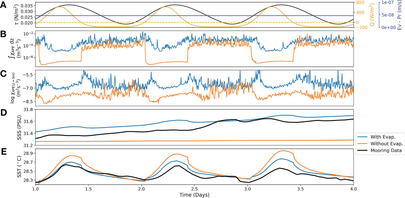
Figure 4 (A) Wind stress magnitude τ (N/m²) (black), net heat flux Q (W/m²) (orange) and evaporation minus precipitation E-P (m/s) (blue). (B) Vertically integrated mixing till 250m for both the cases. (C) Logarithm of mixing plotted for both cases. (D) SSS comparison and (E) SST comparison of both the cases with mooring data.

4 Discussion

Convection resolving large-eddy simulations have been employed to study the upper ocean turbulence and mixing in response to a diurnal forcing of surface fluxes including evaporation, having both temperature and salinity as scalars. Quantifying the associated turbulence and mixing, we have especially focused on the role of evaporation in controlling the SSS and increasing mixing. We present the first evidence for evaporatively caused salt-fingering instability in the near surface layer during daytime. The surface evaporation enhances mixing by almost order of magnitude as compared to the case without evaporation, during daytime. In addition to above, we also show that the changing nature of convection when surface cooling during nighttime is the major contributor towards mixing, while evaporation plays a secondary role. The overall increase in mixing also causes deeper OML, as compared to the case without evaporation. Our simulation results agree well with the mooring observations. The balance between the evaporative flux and the interior mixing dictates the evolution of SSS, and the increased mixing also helps to better predict the SST. The diapycnal diffusivity differs by almost couple of orders of magnitudes during daytime and nighttime, and peaks around 10${-}^1$ m²/s during nighttime. Similarly, the irreversible mixing ${\chi }_{APE}$ and its efficiency $\eta$ are also enhanced during nighttime, reaching values close to 1, which are previously reported in convection dominated systems. Future work concerns including the effects of surface waves, Langmuir turbulence and developing appropriate convective parameterizations for including the evaporative effects on turbulence and mixing within the existing ocean models.

Data availability statement

The datasets presented in this study can be found in online repositories. The names of the repository/repositories and accession number(s) can be found in the article/Supplementary Material.

Author contributions

DF, BG, and DS designed the research problem. DF performed the numerical simulations and analyzed the data. DF, BG, DS, GI wrote the paper. All authors contributed to the article and approved the submitted version.

Funding

DF acknowledges the Prime Minister’s Research Fellows (PMRF) scheme and BG is supported by Australian Research Council Future Fellowship Grant FT180100037. Numerical simulations were conducted on the Australian National Computational Infrastructure, the Australian National University, which is supported by the Commonwealth of Australia. This work is supported by the Ministry of Earth Sciences under India’s National Monsoon Mission.

Conflict of interest

The authors declare that the research was conducted in the absence of any commercial or financial relationships that could be construed as a potential conflict of interest.

Publisher’s note

All claims expressed in this article are solely those of the authors and do not necessarily represent those of their affiliated organizations, or those of the publisher, the editors and the reviewers. Any product that may be evaluated in this article, or claim that may be made by its manufacturer, is not guaranteed or endorsed by the publisher.

Supplementary material

The Supplementary Material for this article can be found online at: https://www.frontiersin.org/articles/10.3389/fmars.2023.1176226/full#supplementary-material

References

Arthur R. S., Venayagamoorthy S. K., Koseff J. R., Fringer O. B. (2017). How we compute n matters to estimates of mixing in stratified flows. J. Fluid Mechanics 831, R2. doi: 10.1017/jfm.2017.679

CrossRef Full Text | Google Scholar

Asher W. E., Jessup A. T., Clark D. (2014). Stable near-surface ocean salinity stratifications due to evaporation observed during strasse. J. Geophysical Research: Oceans 119, 3219–3233. doi: 10.1002/2014JC009808

CrossRef Full Text | Google Scholar

Bouffard D., Boegman L. (2013). A diapycnal diffusivity model for stratified environmental flows. Dynamics Atmospheres Oceans 61, 14–34. doi: 10.1016/j.dynatmoce.2013.02.002

CrossRef Full Text | Google Scholar

Boutin J., Chao Y., Asher W. E., Delcroix T., Drucker R., Drushka K., et al. (2016). Satellite and in situ salinity: understanding near-surface stratification and subfootprint variability. Bull. Am. Meteorological Soc. 97, 1391–1407. doi: 10.1175/BAMS-D-15-00032.1

CrossRef Full Text | Google Scholar

Brainerd K., Gregg M. (1993). Diurnal restratification and turbulence in the oceanic surface mixed layer: 1. observations. J. Geophysical Research: Oceans 98, 22645–22656. doi: 10.1029/93JC02297

CrossRef Full Text | Google Scholar

de Szoeke S. P., Marke T., Brewer W. A. (2021). Diurnal ocean surface warming drives convective turbulence and clouds in the atmosphere. Geophysical Res. Lett. 48, e2020GL091299. doi: 10.1029/2020GL091299

CrossRef Full Text | Google Scholar

Drushka K., Asher W. E., Ward B., Walesby K. (2016). Understanding the formation and evolution of rain-formed fresh lenses at the ocean surface. J. Geophysical Research: Oceans 121, 2673–2689. doi: 10.1002/2015JC011527

CrossRef Full Text | Google Scholar

Drushka K., Gille S. T., Sprintall J. (2014). The diurnal salinity cycle in the tropics. J. Geophysical Research: Oceans 119, 5874–5890. doi: 10.1002/2014JC009924

CrossRef Full Text | Google Scholar

Fairall C., Bradley E. F., Godfrey J., Wick G., Edson J. B., Young G. (1996). Cool-skin and warm-layer effects on sea surface temperature. J. Geophysical Research: Oceans 101, 1295–1308. doi: 10.1029/95JC03190

CrossRef Full Text | Google Scholar

Flament P., Firing J., Sawyer M., Trefois C. (1994). Amplitude and horizontal structure of a large diurnal sea surface warming event during the coastal ocean dynamics experiment. J. Phys. oceanography 24, 124–139. doi: 10.1175/1520-0485(1994)024<0124:AAHSOA>2.0.CO;2

CrossRef Full Text | Google Scholar

Gayen B., Hughes G. O., Griffiths R. W. (2013). Completing the mechanical energy pathways in turbulent rayleigh-bénard convection. Phys. Rev. Lett. 111, 124301. doi: 10.1103/PhysRevLett.111.124301

PubMed Abstract | CrossRef Full Text | Google Scholar

Gregg M. C. (2021). Ocean mixing (Cambridge University Press). 78–79.

Google Scholar

Hughes K. G., Moum J. N., Shroyer E. L. (2020a). Evolution of the velocity structure in the diurnal warm layer. J. Phys. Oceanography 50, 615–631. doi: 10.1175/JPO-D-19-0207.1

CrossRef Full Text | Google Scholar

Hughes K. G., Moum J. N., Shroyer E. L. (2020b). Heat transport through diurnal warm layers. J. Phys. Oceanography 50, 2885–2905. doi: 10.1175/JPO-D-20-0079.1

CrossRef Full Text | Google Scholar

Imberger J. (1985). The diurnal mixed layer 1. Limnology oceanography 30, 737–770. doi: 10.4319/lo.1985.30.4.0737

CrossRef Full Text | Google Scholar

Ivey G. N., Bluteau C. E., Gayen B., Jones N. L., Sohail T. (2021). Roles of shear and convection in driving mixing in the ocean. Geophysical Res. Lett. 48, e2020GL089455. doi: 10.1029/2020GL089455

CrossRef Full Text | Google Scholar

Ivey G., Imberger J. (1991). On the nature of turbulence in a stratified fluid. part i: the energetics of mixing. J. Phys. Oceanography 21, 650–658. doi: 10.1175/1520-0485(1991)021<0650:OTNOTI>2.0.CO;2

CrossRef Full Text | Google Scholar

Lombardo C., Gregg M. (1989). Similarity scaling of viscous and thermal dissipation in a convecting surface boundary layer. J. Geophysical Research: Oceans 94, 6273–6284. doi: 10.1029/JC094iC05p06273

CrossRef Full Text | Google Scholar

Matthews A. J., Baranowski D. B., Heywood K. J., Flatau P. J., Schmidtko S. (2014). The surface diurnal warm layer in the indian ocean during cindy/dynamo. J. Climate 27, 9101–9122. doi: 10.1175/JCLI-D-14-00222.1

CrossRef Full Text | Google Scholar

Moulin A. J., Moum J. N., Shroyer E. L. (2018). Evolution of turbulence in the diurnal warm layer. J. Phys. Oceanography 48, 383–396. doi: 10.1175/JPO-D-17-0170.1

CrossRef Full Text | Google Scholar

Moum J., Lien R.-C., Perlin A., Nash J., Gregg M., Wiles P. (2009). Sea Surface cooling at the equator by subsurface mixing in tropical instability waves. Nat. Geosci. 2, 761–765. doi: 10.1038/ngeo657

CrossRef Full Text | Google Scholar

Nagai T., Inoue R., Tandon A., Yamazaki H. (2015). Evidence of enhanced double-diffusive convection below the main stream of the k uroshio e xtension. J. Geophysical Research: Oceans 120, 8402–8421. doi: 10.1002/2015JC011288

CrossRef Full Text | Google Scholar

Osborn T. R., Cox C. S. (1972). Oceanic fine structure. Geophysical Fluid Dynamics 3, 321–345. doi: 10.1080/03091927208236085

CrossRef Full Text | Google Scholar

Paulson C. A., Simpson J. J. (1977). Irradiance measurements in the upper ocean. J. Phys. Oceanography 7, 952–956. doi: 10.1175/1520-0485(1977)007<0952:IMITUO>2.0.CO;2

CrossRef Full Text | Google Scholar

Pham H. T., Sarkar S., Winters K. B. (2013). Large-Eddy simulation of deep-cycle turbulence in an equatorial undercurrent model. J. Phys. Oceanography 43, 2490–2502. doi: 10.1175/JPO-D-13-016.1

CrossRef Full Text | Google Scholar

Pham H. T., Smyth W. D., Sarkar S., Moum J. N. (2017). Seasonality of deep cycle turbulence in the eastern equatorial pacific. J. Phys. Oceanography 47, 2189–2209. doi: 10.1175/JPO-D-17-0008.1

CrossRef Full Text | Google Scholar

Price J. F., Weller R. A., Pinkel R. (1986). Diurnal cycling: observations and models of the upper ocean response to diurnal heating, cooling, and wind mixing. J. Geophysical Research: Oceans 91, 8411–8427. doi: 10.1029/JC091iC07p08411

CrossRef Full Text | Google Scholar

Rosevear M. G., Gayen B., Galton-Fenzi B. K. (2021). The role of double-diffusive convection in basal melting of antarctic ice shelves. Proc. Natl. Acad. Sci. 118, e2007541118. doi: 10.1073/pnas.2007541118

CrossRef Full Text | Google Scholar

Ruddick B. (1983). A practical indicator of the stability of the water column to double-diffusive activity. Deep Sea Res. Part A. Oceanographic Res. Papers 30, 1105–1107. doi: 10.1016/0198-0149(83)90063-8

CrossRef Full Text | Google Scholar

Sarkar S., Pham H. T. (2019). Turbulence and thermal structure in the upper ocean: turbulence-resolving simulations. Flow Turbulence Combustion 103, 985–1009. doi: 10.1007/s10494-019-00065-5

CrossRef Full Text | Google Scholar

Saunders P. M. (1967). The temperature at the ocean-air interface. J. Atmospheric Sci. 24, 269–273. doi: 10.1175/1520-0469(1967)024<0269:TTATOA>2.0.CO;2

CrossRef Full Text | Google Scholar

Shay T. J., Gregg M. (1986). Convectively driven turbulent mixing in the upper ocean. J. Phys. Oceanography 16, 1777–1798. doi: 10.1175/1520-0485(1986)016<1777:CDTMIT>2.0.CO;2

CrossRef Full Text | Google Scholar

Smyth W., Moum J., Li L., Thorpe S. (2013). Diurnal shear instability, the descent of the surface shear layer, and the deep cycle of equatorial turbulence. J. Phys. Oceanography 43, 2432–2455. doi: 10.1175/JPO-D-13-089.1

CrossRef Full Text | Google Scholar

Sohail T., Gayen B., Hogg A. M. (2018). Convection enhances mixing in the southern ocean. Geophysical Res. Lett. 45, 4198–4207. doi: 10.1029/2018GL077711

CrossRef Full Text | Google Scholar

Soloviev A., Lukas R. (1997). Observation of large diurnal warming events in the near-surface layer of the western equatorial pacific warm pool. Deep Sea Res. Part I: Oceanographic Res. Papers 44, 1055–1076. doi: 10.1016/S0967-0637(96)00124-0

CrossRef Full Text | Google Scholar

Stull R. B. (1988). An introduction to boundary layer meteorology Vol. vol. 13 (Springer Science & Business Media). 255.

Google Scholar

Sui C., Li X., Lau K., Adamec D. (1997). Multiscale air–sea interactions during toga coare. Monthly weather Rev. 125, 448–462. doi: 10.1175/1520-0493(1997)125<0448:MASIDT>2.0.CO;2

CrossRef Full Text | Google Scholar

Wallace J., Hartranft F. (1969). Diurnal wind variations, surface to 30 kilometers. Monthly Weather Rev. 97, 446–455. doi: 10.1175/1520-0493(1969)097<0446:DWVSTK>2.3.CO;2

CrossRef Full Text | Google Scholar

Weller R. A., Farrar J. T., Buckley J., Mathew S., Venkatesan R., Lekha J. S., et al. (2016). Air-sea interaction in the bay of bengal. Oceanography 29, 28–37. doi: 10.5670/oceanog.2016.36

CrossRef Full Text | Google Scholar

Weller R., Farrar J., Seo H., Prend C., Sengupta D., Lekha J. S., et al. (2019). Moored observations of the surface meteorology and air–sea fluxes in the northern bay of bengal in 2015. J. Climate 32, 549–573. doi: 10.1175/JCLI-D-18-0413.1

CrossRef Full Text | Google Scholar

Wenegrat J. O., McPhaden M. J. (2015). Dynamics of the surface layer diurnal cycle in the equatorial atlantic ocean (0, 23 w). J. Geophysical Research: Oceans 120, 563–581. doi: 10.1002/2014JC010504

CrossRef Full Text | Google Scholar

Wijesekera H. W., Wang D. W., Jarosz E. (2020). Dynamics of the diurnal warm layer: surface jet, high-frequency internal waves, and mixing. J. Phys. Oceanography 50, 2053–2070. doi: 10.1175/JPO-D-19-0285.1

CrossRef Full Text | Google Scholar

Wykes M. S. D., Hughes G. O., Dalziel S. B. (2015). On the meaning of mixing efficiency for buoyancy-driven mixing in stratified turbulent flows. J. Fluid Mechanics 781, 261–275. doi: 10.1017/jfm.2015.462

CrossRef Full Text | Google Scholar

Yan Y., Zhang L., Yu Y., Chen C., Xi J., Chai F. (2021). Rectification of the intraseasonal sst variability by the diurnal cycle of sst revealed by the global tropical moored buoy array. Geophysical Res. Lett. 48, e2020GL090913. doi: 10.1029/2020GL090913

CrossRef Full Text | Google Scholar

Yu L. (2010). On sea surface salinity skin effect induced by evaporation and implications for remote sensing of ocean salinity. J. Phys. oceanography 40, 85–102(. doi: 10.1175/2009JPO4168.1

CrossRef Full Text | Google Scholar