Analysis of mooring-observed bottom current on the northern continental shelf of the South China Sea

The bottom current is an important component of the three-dimensional ocean circulation, which is of significance for the safeties of ocean bottom engineering and facilities, the research on sediment and pollutant transports, and the ecological environment. Due to the lack of observation data, research on the bottom current in the South China Sea (SCS) has been limited. This study systematically analyzes bottom currents from 0.5 to 5 m above the seafloor based on 20-month-long mooring observations on the shelf slope west of the Dongsha Atoll. The spectral analysis results indicate that currents induced by the internal tides and the internal solitary waves (ISWs) comprise dominant constituents of bottom currents with velocity amplitudes up to O(50–90) cm/s. Dominant internal tide-induced bottom currents of the velocity amplitude of O(50) cm/s occupy 53% of the total horizontal kinetic energy. The pulsating ISW-induced bottom currents reach a maximum amplitude of 93 cm/s, which has intrinsic relation to the amplitude of the ISWs, according to the soliton propagation speed solutions of the Korteweg–De Vries (KdV) equation. The background bottom current is strongest in winter, followed by spring, and weak in summer and autumn, which is closely correlated with the behavior of mesoscale eddies. These results are of significance for understanding the dynamics of the bottom boundary layer.

1 Introduction

As an important component of the three-dimensional ocean circulation, the bottom current is of significance particularly for the safeties of ocean bottom engineering and facilities, the research on sediment and pollutant transports, and the ecological environment on the continental shelf (Connolly et al., 2020; Zhu and Liang, 2020). According to long-term observations on the mid-Atlantic continental shelf, Butman et al. (1979) found that the storm-induced bottom current reached 30 cm/s, which is strong enough to resuspend and redistribute sediments on the seafloor. Since then, previous investigations have revealed that sedimentary systems, including sediment formation and transportation, are closely linked to bottom currents (Lei et al., 2007; Zheng and Yan, 2012; Chen et al., 2016; Jia et al., 2019). Meanwhile, the strong bottom currents may result in a serious threat to the safety of underwater operations, such as remote-operated vehicle (ROV) operations and submarine pipeline docking during exploitation of offshore oil and gas resources. However, in contrast to surface currents that are easily derived from abundant satellite data and cruise observations, the understanding of bottom currents is restricted by lack of observational data.

The South China Sea (SCS) is the largest semi-enclosed marginal sea of the West Pacific. Previous studies have figured out the characteristics of general bottom circulation in the SCS, i.e., there is a cyclonic circulation of a magnitude of O(0–10) cm/s, which is stronger in summer and weaker in winter (Li and Qu, 2006; Wang et al., 2011; Lan et al., 2013; Lan et al., 2015). In recent years, research on bottom currents in the SCS has gained important progress. Liu et al. (2011) observed the strong bottom current induced by the near-inertial internal wave generated by typhoon Pabuk using the observations of 300K acoustic Doppler current profiler (ADCP) installed on the oil platform. Their results show that the maximum bottom current reached nearly 1 m/s at 12 m above the bottom on the northern continental slope of the SCS. Wu et al. (2016) analyzed the bottom currents at a depth of approximately 1,000 m in and around a submarine valley on the northern continental slope of the SCS. Their results show that bottom currents are strongly conditioned by the topography, flowing along the valley axis or isobaths. The bottom current on the open slope is distinct from that in the submarine valley. The former is dominated by the diurnal cycle, while the latter is dominated by the semidiurnal cycle. Li et al. (2019) found that near-bottom current velocities southeast of Dongsha Atoll are between 20 and 30 cm/s, of which the tidal currents occupy about 70%.

Satellite and cruise observations have revealed that the northern SCS is featured by frequent occurrence of internal waves (Jackson, 2007; Zheng et al., 2007; Wang et al., 2012; Chen et al., 2018; Chen et al., 2019; Zheng et al., 2020). The coincidence of a strong but shallow thermocline in the Luzon Strait and the strong tidal currents results in the generation of large-amplitude internal tides that radiate away from the Luzon Strait into both the SCS and the West Pacific (Simmons et al., 2011). Based on satellite altimeter sea surface height (SSH) data, Zhao (2014) found that internal tides K1 and O1 in the SCS mainly propagate southwestward between 200° and 215° from the true north. The westward M2 internal tide bifurcates into two beams. The northwestward beam is coincident with the frequently occurring internal solitary waves (ISWs), implying their causative relation. It is believed that the westward-propagating internal tides from the Luzon Strait steepen and evolve into large-amplitude ISWs near the Dongsha Atoll (Zhao et al., 2004; Farmer et al., 2011; Simmons et al., 2011; Alford et al., 2015). According to 1-year-long mooring data, Chen et al. (2019) found that the ISWs on the shelf slope northwest of the Dongsha Atoll occur frequently in the forms of mode-1 single solitons and wave packets, which are well described by the solutions of the Korteweg–De Vries (KdV) equation.

Owing to two decades of efforts, the understanding of the generation mechanism and propagation characteristics of ISWs in the SCS has gradually become clear. However, previous studies mostly focused on their impacts on the upper ocean but few on the bottom current. This is mainly because of difficulties to measure the current data near the seabed. Especially, bottom current data within 1 m above the seafloor have not been available. This study analyzes strong bottom currents induced by internal tides and ISWs in the SCS based on 20-month-long mooring observations on the shelf slope west of the Dongsha Atoll.

This paper is organized as follows. The Data and Methods section describes the cruise and mooring observation programs and data-processing methods. The Results and Discussion section analyzes the features of bottom currents induced by the internal tides and the ISWs as well as the seasonal variation of background bottom current. The Conclusions section gives the main analysis results of bottom currents on the northern continental shelf of South China Sea based on mooring observations.

2 Data and methods

2.1 Mooring observation

The mooring station is located 20.8°N 115.8°E in the west of the Dongsha Atoll on the northern shelf slope of the SCS with a depth of 330 m as shown in Figure 1A. The mooring, which was specially designed to observe bottom currents, was deployed to measure the current velocity, temperature, and salinity from 1 April 2020 to 6 November 2021. From the depth of 20–320 m, a thermistor chain consisting of conductivity-temperature-depth (CTD) instruments and temperature loggers at every 10 m was attached to the mooring to monitor the temperature and the salinity. The current velocity from 20 to 100 m was sampled via a 40-inch vitreous mounted upward-looking 300-kHz ADCP at a depth of 105 m. At the depth of 323 m, an upward-looking 150-kHz ADCP and a downward-looking 1-MHz ADCP are installed back-to-back in a 49-inch vitreous float. The current velocities between 100 and 320 m were sampled by the 150-kHz ADCP. The 300-kHz and 150-kHz ADCPs sampled every 2 min with a bin size of 4 m. The bottom current from 0.5 to 5 m above the seafloor was sampled by the 1-MHz ADCP with 0.2-m bins every 2 min. The valid bin numbers of the 300-kHz, 150-kHz, and 1-MHz ADCPs are 21, 55, and 26, respectively. There are 45 pings in an ensemble for the 300-kHz ADCP and 60 pings in an ensemble for the 150-kHz and 1-MHz ADCPs. The standard deviations of the 300-kHz, 150-kHz, and 1-MHz ADCPs are 0.53, 0.90, and 1.69 cm/s, respectively. Especially, a round cake lead anchor with a height of not more than 10 cm was used to avoid the impacts on in situ bottom current measurements induced by the high anchor of the mooring. The design drawing of the mooring is shown in Figure 1B. The observation of the 1-MHz ADCP was terminated on 17 September 2021 due to battery failure. Therefore, data from 17 full months from 1 April 2020 to 31 August 2021 are used for the statistical analysis of bottom current in this paper. Here, we define the current within 1 m from the bottom observed by the 1-MHz ADCP as the bottom current.

FIGURE 1

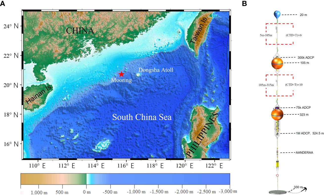
Figure 1 (A) Study area and mooring station (red star) and (B) mooring design drawing.

2.2 Decomposition of the currents

2.2.1 Current velocity induced by internal tides

The horizontal current $u$ observed by ADCP can be written as follows:

$$\overrightarrow{u}=\overrightarrow{u_{bt}}+\overrightarrow{u_{IT}},$$

where $\overrightarrow{u_{bt}}=\frac{1}{H}{\int }_{-\text{H}}^{0}u\text{dz}$ is the barotropic current, and $\overrightarrow{u_{IT}}$ is the internal tidal current

$\begin{array}{ll}\overrightarrow{u_{IT}}=\overrightarrow{u_{D1}}+\overrightarrow{u_{D2}}& (2)\end{array}$

where $\overrightarrow{u_{D1}}$ and $\overrightarrow{u_{D2}}$ are components of the diurnal [0.79d 1.15d] and semidiurnal [1.64d 2.3d] tidal bands.

Internal tides are strongly modulated by background conditions, such as stratification variability and mesoscale processes (Baines, 1982; Park and Watts, 2006). As a result, part of the internal tidal energy may exhibit intermittent features, occur at frequencies outside the deterministic tidal frequencies, and become incoherent with astronomical forcing (van Haren, 2004). The deterministic coherent internal tides can be written as follows (van Haren, 2003):

$\begin{array}{ll}{u}_c={\sum }_k{U}_{k}cos({\phi }_k+{\omega }_{k}t)& (3)\end{array}$

$${\omega }_k=Q_1, O_1, P_1, K_1, N_2, M_2, S_2, K_2,$$

where $U_k$ is the amplitude, and ${\phi }_k$ is the phase. The components in Eq. 2 are chosen because they are the dominant components in tidal motions in the SCS (Zu et al., 2008; Xie et al., 2013; Shang et al., 2015). They can be extracted from the ADCP-observed current by applying a harmonic analysis toolbox, t_tide (Pawlowicz et al., 2002).

Then, the incoherent internal tides are defined as follows:

$\begin{array}{ll}\overrightarrow{u_{ic}}=\overrightarrow{u_{IT}}-\overrightarrow{u_c}& (4)\end{array}$

2.2.2 Current velocity induced by internal solitary waves

The horizontal and vertical velocity components induced by ISWs are calculated by the following:

$\begin{array}{ll}\overrightarrow{u_{ISW}}=\overrightarrow{u}-\overrightarrow{u_0}& (5)\end{array}$

$\begin{array}{ll}\overrightarrow{w_{ISW}}=\overrightarrow{w}-\overrightarrow{w_0}-\overrightarrow{w_c}& (6)\end{array}$

where $\overrightarrow{u}$, $\overrightarrow{w}$ are the total horizontal and vertical velocity components measured by the ADCP, respectively; $\overrightarrow{u_0}$, $\overrightarrow{w_0}$ are the background horizontal and vertical velocity components, which are calculated by averaging the velocity data measured by the ADCP at 30 min before the ISW arrival; and the vertical motion of ADCP is corrected by $\overrightarrow{w_c}$, which is calculated by $\frac{d_2-d_1}{t_2-t_1}$. $d_1$ and $d_2$ are the depths at the time $t_1$ and $t_2$ measured by CTD attached to the ADCP.

2.3 The Korteweg–De Vries theory

The propagation process of ISWs can be described by the KdV equation. In continuous stratified fluids, the KdV equation can be written as follows (Pelinovsky et al., 2007):

$\begin{array}{ll}\frac{\partial {\text{η}}_n}{\partial \text{t}}+c_n\frac{\partial {\text{η}}_n}{\partial \text{x}}+{\alpha }_n{\text{η}}_n\frac{\partial {\text{η}}_n}{\partial \text{x}}+{\beta }_n\frac{{\partial }^3{\text{η}}_n}{\partial {\text{x}}^3}=0& (7)\end{array}$

where $c_n$, ${\alpha }_n$, ${\beta }_n$ are the linear wave speed, nonlinear coefficient, and dispersion coefficient of mode n, respectively. Here,

$\begin{array}{ll}{\alpha }_n=\frac{3}{2}{\int }_{-H}^0{(c_n-U)}^2\frac{d^3{\Phi }_n}{d{z}^3}dz/{\int }_{-H}^0(c_n-U)\frac{d^2{\Phi }_n}{d{z}^2}dz& (8)\end{array}$

$\begin{array}{ll}{\beta }_n=\frac{1}{2}{\int }_{-H}^0{(c_n-U)}^2{\Phi }_n^{2}dz/{\int }_{-H}^0(c_n-U)\frac{d^2{\Phi }_n}{d{z}^2}dz& (9)\end{array}$

where $\text{U}(\text{z})$ is the background shear current, which is calculated by averaging the velocity data measured by the ADCP at 30 min before the ISW arrival; ${\Phi }_n$ is the vertical structure of vertical displacement, which can be described as the Taylor–Goldstein (T-G) equation (Holloway et al., 1997; Grimshaw et al., 2004):

$\begin{array}{ll}\frac{\text{d}}{dz}[{(c_n-U)}^2\frac{d{\Phi }_n}{dz}]+N^2(z){\Phi }_n=0& (10)\end{array}$

$\begin{array}{ll}\Phi (-H)=\Phi (0)=0& (11)\end{array}$

where $N^2(\text{z})=-\frac{g}{\rho }\frac{d\rho }{dz}$ is the buoyancy frequency. Equations 8 and 9 can be solved by the matrix method (Chen et al., 2019).

Equation 5 has a single soliton solution in the form of the following:

$\begin{array}{ll}{\eta }_n(x,t)={\eta }_{0,n}sec{h}^2(\frac{x-C_{n}t}{{\Delta }_n})& (12)\end{array}$

where ${\eta }_{0,n}$ is the amplitude, $C_n$ is the nonlinear phase speed, and ${\Delta }_n$ is the horizontal characteristic half width, i.e.,

$\begin{array}{ll}{C}_n=c_n+\frac{{\alpha }_n{\text{η}}_{0,n}}{3}& (13)\end{array}$

$\begin{array}{ll}{\Delta }_n=\sqrt{\frac{12{\beta }_n}{{\alpha }_n{\text{η}}_{0,n}}}& \text{. (14)}\end{array}$

For a two-layer ocean, we have the following:

$\begin{array}{ll}{c}_n={[\frac{g({\rho }_2-{\rho }_1)h_1{h}_2}{{\rho }_2{h}_1+{\rho }_1{h}_2}]}^{1/2}& \text{(14a)}\end{array}$

which is defined as the linear phase speed,

$\begin{array}{ll}{\alpha }_n=\frac{3}{2}\frac{c}{h_1{h}_2}\frac{{\rho }_2{h}_1^2-{\rho }_1{h}_2^2}{{\rho }_2{h}_1+{\rho }_1{h}_2}& \text{(14b)}\end{array}$

which is defined as the nonlinear coefficient, and

$\begin{array}{ll}{\beta }_n=\frac{c{h}_1{h}_2}{6}\frac{{\rho }_1{h}_1+{\rho }_2{h}_2}{{\rho }_2{h}_1+{\rho }_1{h}_2}& \text{(14c)}\end{array}$

which is a measure of dispersion. Here, h₁ and h₂ are the thicknesses of the upper and lower layers, respectively, and the water densities are ρ₁ and ρ₂, which are uniform within the layer.

Thus, for a multi-solitary wave field, the vertical displacement $\eta (x,z,t)$ can be written as follows:

$\begin{array}{ll}\eta (x,z,t)={\displaystyle \sum _n^{}}{\eta }_n(x,t){\Phi }_n(z)& (15)\end{array}$

Because the amplitude of the ISW is ${\eta }_{0,n}$, ${\Phi }_n(z)$ should be normalized as ${\Phi }_{max}=1$.

According to the relationship of the vertical displacement and the vertical velocity,

$\begin{array}{ll}w(x,z,t)=\frac{d\eta (x,z,t)}{dt}& (16)\end{array}$

the vertical velocity $w(x,z,t)$ can be written in the form of the following:

$\begin{array}{ll}w(x,z,t)={\displaystyle \sum _n^{}}{w}_n(x,t)W_n(z)& (17)\end{array}$

Here, the vertical structure of the vertical velocity $W_n(z)={\Phi }_n(z)$, and $w_n(x,t)$ can be written as follows:

$\begin{array}{ll}{w}_n(x,t)=-\frac{2{\eta }_{0,n}{C}_n}{{\Delta }_n}sec{h}^2(\frac{x-C_{n}t}{{\Delta }_n})\text{tanh}(\frac{x-C_{n}t}{{\Delta }_n})& (18)\end{array}$

For the horizontal velocity $u(x,z,t)$, horizontal and vertical components can be treated individually in the form of the following:

$\begin{array}{ll}u(x,z,t)={\displaystyle \sum _n^{}}{u}_n(x,t)U_n(z)& (19)\end{array}$

where $U(z)$ is the vertical structure of the horizontal velocity.

In the (x-z) two-dimensional model, the continuity equation can be written as follows:

$\begin{array}{ll}\frac{\partial u}{\partial \text{x}}=-\frac{\partial w}{\partial z}& (20)\end{array}$

Then, according to Eqs. 15 and 16, $u_n(x,\text{z},t)$ can be written as follows:

$\begin{array}{ll}{u}_n(x,z,t)={\eta }_{0,n}{C}_{n}sec{h}^2(\frac{x-C_{n}t}{{\Delta }_n})\frac{d{\Phi }_n}{dz}& (21)\end{array}$

When taking $z=-H$, due to the influence of the bottom boundary, both vertical displacement and vertical velocity are zero; and the horizontal bottom current can be calculated as follows:

$\begin{array}{ll}{V}_b={\eta }_{0,n}{C}_{n}sec{h}^2(\frac{x-C_{n}t}{{\Delta }_n})\frac{d{\Phi }_n}{dz}{|}_{Z=-H}& (22)\end{array}$

When $sec{h}^2(\frac{x-C_{n}t}{{\Delta }_n})=1$, i.e., the trough or peak of the ISW appears, the bottom current induced by the ISW reaches the maximum. Then, the maximum bottom current can be expressed as follows:

$\begin{array}{ll}{V}_{b, max}=k{\eta }_{0,n}{C}_n& (23)\end{array}$

where $k=\frac{d{\Phi }_n}{dz}{|}_{Z=-H}$.

3 Results and discussion

3.1 Bottom current induced by internal tides

To identify periodic motions in the bottom current, the spectral analysis is applied for the extracted barotropic and baroclinic currents from observation data according to Eq. 1. Figure 2A shows the vertical distribution of the power spectral density derived from mooring-measured current velocity data. One can see that diurnal internal tides O1 and K1 and semidiurnal internal tides M2 and S2 are the dominant constituents for the whole water profile. The energy of the near-inertial waves is comparable to that of the internal tides in the upper ocean. For the bottom current, the energy density of the baroclinic component (red line in Figure 2B) is much higher than that of the barotropic component (blue line). Meanwhile, the diurnal internal tide and semidiurnal internal tide are the main components of the bottom currents, consistent with the results shown in Figure 2A. To further confirm this point, we extract the diurnal internal tide and semidiurnal internal tide by a band-pass filter and compare them with observed bottom currents. Figure 3 shows the results of January 2021. One can see that the variety of bottom currents induced by the internal tides is in good agreement with the ADCP-measured current. However, fluctuations of the bottom current caused by the barotropic tide are remarkably smaller than that of the ADCP-measured current, implying that baroclinic currents caused by diurnal and semidiurnal internal tides are the dominant constituents of the bottom current rather than the barotropic tide.

FIGURE 2

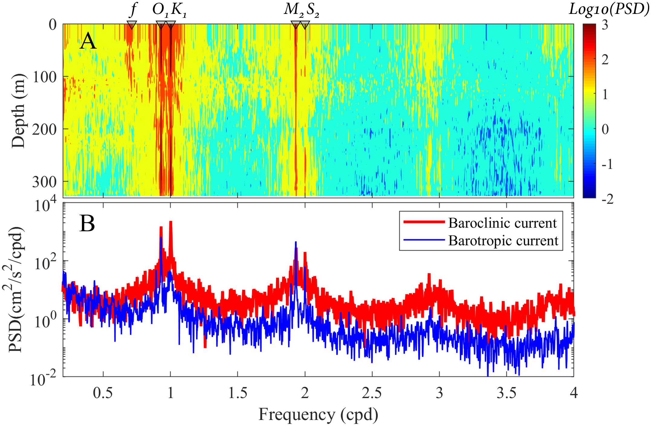
Figure 2 (A) Vertical distribution of the power spectral density of the zonal baroclinic current (f: inertial frequency of 0.713 cpd; O₁: 0.9295 cpd; K₁: 1.0027 cpd; M₂: 1.9323 cpd; S₂: 2 cpd). (B) Power density spectra of the zonal bottom current. PSD, power spectral density.

FIGURE 3

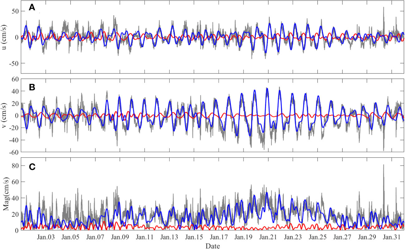
Figure 3 Time series of the bottom current. (A–C) Zonal and meridional velocities and velocity amplitude. Gray, blue, and red lines represent the measured velocity, the velocity induced by diurnal and semidiurnal internal tides and barotropic tide, respectively. u, zonal velocity; v, meridional velocity; Mag, velocity amplitude.

Figure 4 shows the monthly distribution of the maximum and average bottom currents induced by internal tides from August 2020 to August 2021. One can see that bottom currents induced by internal tides flow northwestward in winter and southeastward in summer as shown in Figure 4A. Figure 4B shows the maximum and average absolute values of bottom currents induced by internal tides peaked in January 2021 with a maximum value of about 50 cm/s and an average value of 16 cm/s.

FIGURE 4

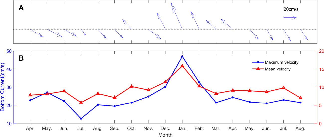
Figure 4 Monthly distribution of the maximum and average bottom currents induced by internal tides. (A) Maximum horizontal bottom current vectors. (B) Maximum and average absolute values of bottom currents.

Figure 5A shows the horizontal kinetic energy proportion of the internal tide current to the total bottom current. One can see that in the total horizontal kinetic energy of the bottom current, that of the internal tide accounts for more than 52% on average, of which the proportion is highest in January, reaching 76%, and the lowest is 39% in July 2020. The diurnal internal tide is the dominant component with an average proportion of 81%. On the other hand, Figure 5B shows that when the internal tides are strongest in January, the proportion of the semidiurnal internal tide also peaks, indicating that the semidiurnal internal tide plays a positive role in strengthening the internal tides in winter. The monthly distribution of coherent and incoherent component proportions in the internal tides is shown as green and gray bars in Figures 5B, C. One can see that the coherent internal tide dominates with an average proportion of 63%, while the incoherent internal tide accounts for 37%. The average coherent and incoherent components of the diurnal and semidiurnal internal tides are 66%, 53% and 34%, 47%, respectively. In winter, the incoherent component of the diurnal internal tides significantly intensifies, reaching a peak of a proportion of 60% in January. In contrast, the incoherent semidiurnal tide gradually weakens, and a trough of a proportion of 26% occurs in January. In the semidiurnal internal tide, the incoherent component accounts for 47%, indicating that nearly half of semidiurnal internal tides is transmitted from other sea areas. Previous studies have shown that nonlinear steepening during the westward propagation of the semidiurnal internal tide in the Luzon Strait is one of the main mechanisms for the generation of ISWs in the SCS (Zhao, 2014). Compared to other seasons, the incoherent component of the semidiurnal internal tide in winter is the lowest, corresponding to the lowest occurrence frequency of ISWs in winter. These results provide evidence for the link of generation of ISWs in the SCS with the semidiurnal internal tide.

FIGURE 5

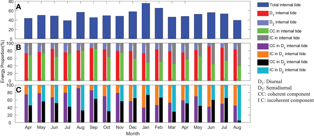
Figure 5 Monthly distributions of bottom current horizontal kinetic energy proportion. (A) The proportion of the horizontal kinetic energy induced by internal tides in the total horizontal kinetic energy. (B) Diurnal, semidiurnal, coherent, and incoherent internal tide horizontal kinetic energy proportions in the total internal tide horizontal kinetic energy. (C) Coherent and incoherent component proportions in the diurnal internal tide and semidiurnal internal tide currents.

3.2 Bottom current induced by internal solitary waves

As shown in Figures 3, 6A, besides the internal tides, there are many abrupt maxima-like spikes in the bottom current time series. Taking the spike in the red dotted box in Figure 6A as an example, Figures 6B–E show the vertical profile characteristics of the temperature and the current velocities. One can see that the isotherms present as a single concave wave with a maximum amplitude of 110 m. The vertical distribution patterns of the zonal and the meridional velocities appear as a distinct two-layer structure with a demarcation depth of 150 m. In the layer above 150 m, the horizontal velocity is northwestward. On the contrary, in the lower layer, it is southeastward. Vertically, there are strong downward and upward currents before and after the passage of the single concave wave, respectively. These characteristics indicate that this is a typical mode-1 ISW (Chen et al., 2019). When the ISW occurs, the bottom velocity suddenly increases from 20 to 80 cm/s as shown in Figure 6F.

FIGURE 6

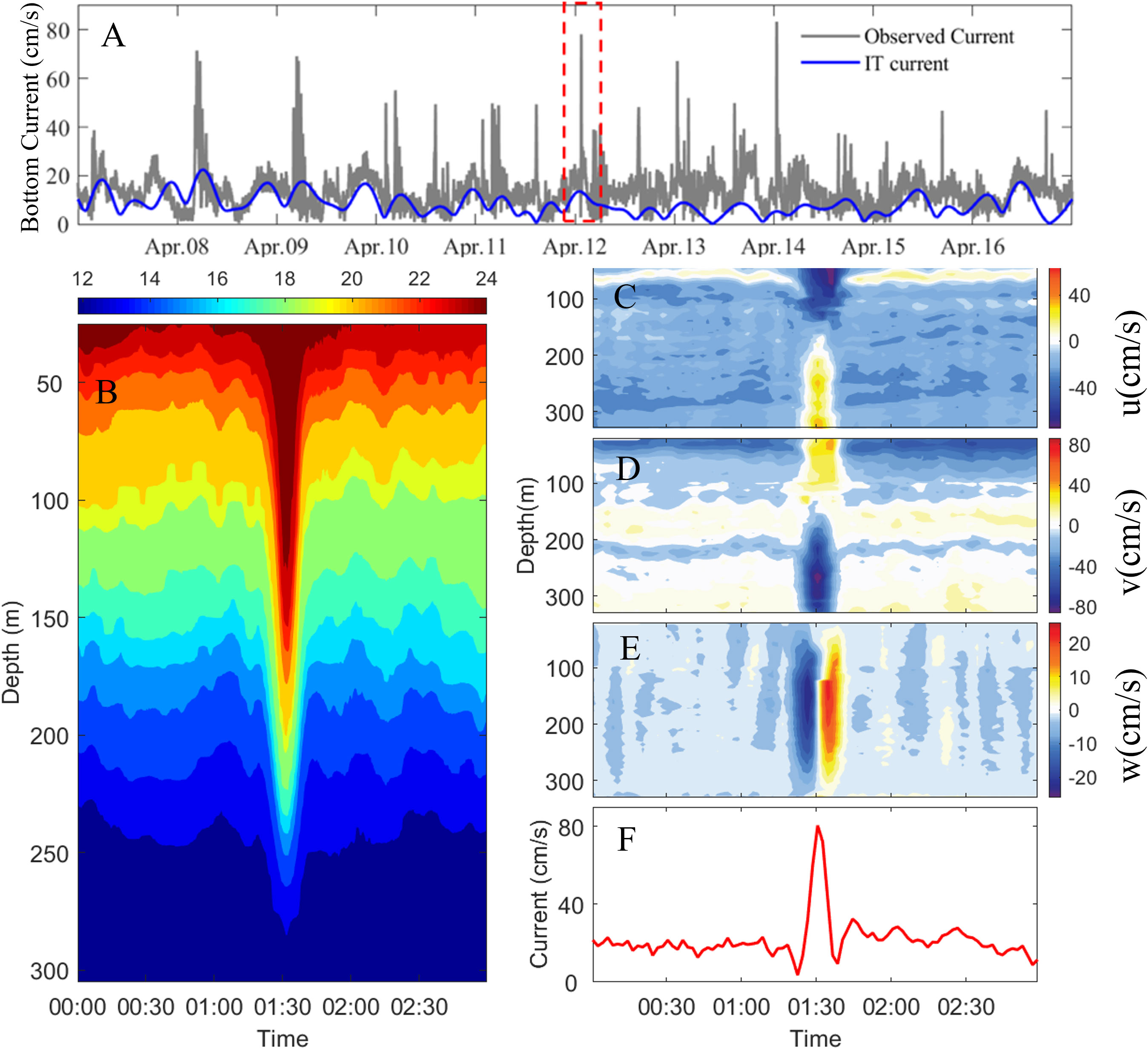
Figure 6 Bottom current induced by ISW observed on 12 April 2020. (A) Time series of bottom current from 7 to 17 April 2020. Panels (B–F) represent the temperature, zonal velocity, meridional velocity, vertical velocity, and the bottom current signals of the ISW in the red dashed box of panel A, respectively. IT, Internal tide; u, zonal velocity; v, meridional velocity; w, vertical velocity.

Figure 7A shows the monthly distribution of the ISW occurrence. One can see that the occurrence frequency is high in summer, low in winter, followed by spring and autumn, which is consistent with the findings of Chen et al. (2019) and Zheng et al. (2007). The occurrence frequency of bottom current exceeding 30 cm/s induced by ISWs accounts for 40% and that exceeding 50 cm/s for 9%. There are eight ISWs inducing extreme bottom currents exceeding 80 cm/s. Figure 8B shows the monthly distribution of the maximum velocity value (blue line) and the mean maximum value (mean value of the maximum velocities) (red line) induced by ISWs. As shown in Figure 7B, the strongest bottom current as large as 93 cm/s (down to 1 m above the seafloor) appears in November and exceeds 50 cm/s in all other months. The mean maximum value is about 30 cm/s, and the maximum value appears in January, which may result from that the pycnocline depth is deeper in winter.

FIGURE 7

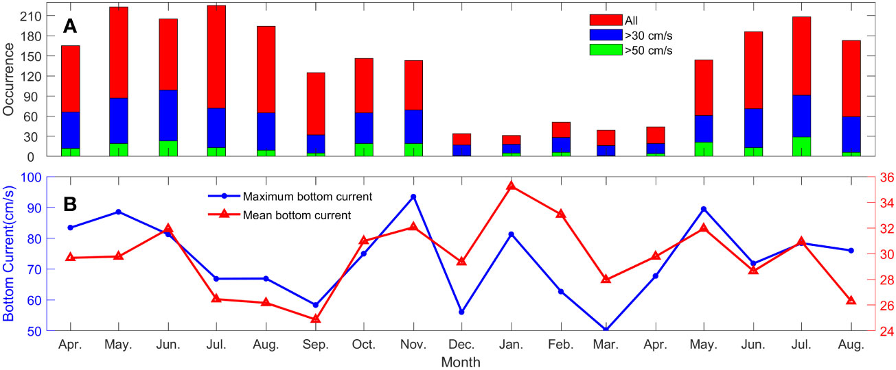
Figure 7 (A) Monthly distribution of the ISW occurrence. The histogram heights represent the occurrence counts of all ISWs (red), ISWs with bottom current exceeding 30 cm/s (blue), and ISWs with bottom current exceeding 50 cm/s (green). (B) The maximum velocity (blue line) and the mean maximum velocity (red line) induced by ISWs.

FIGURE 8

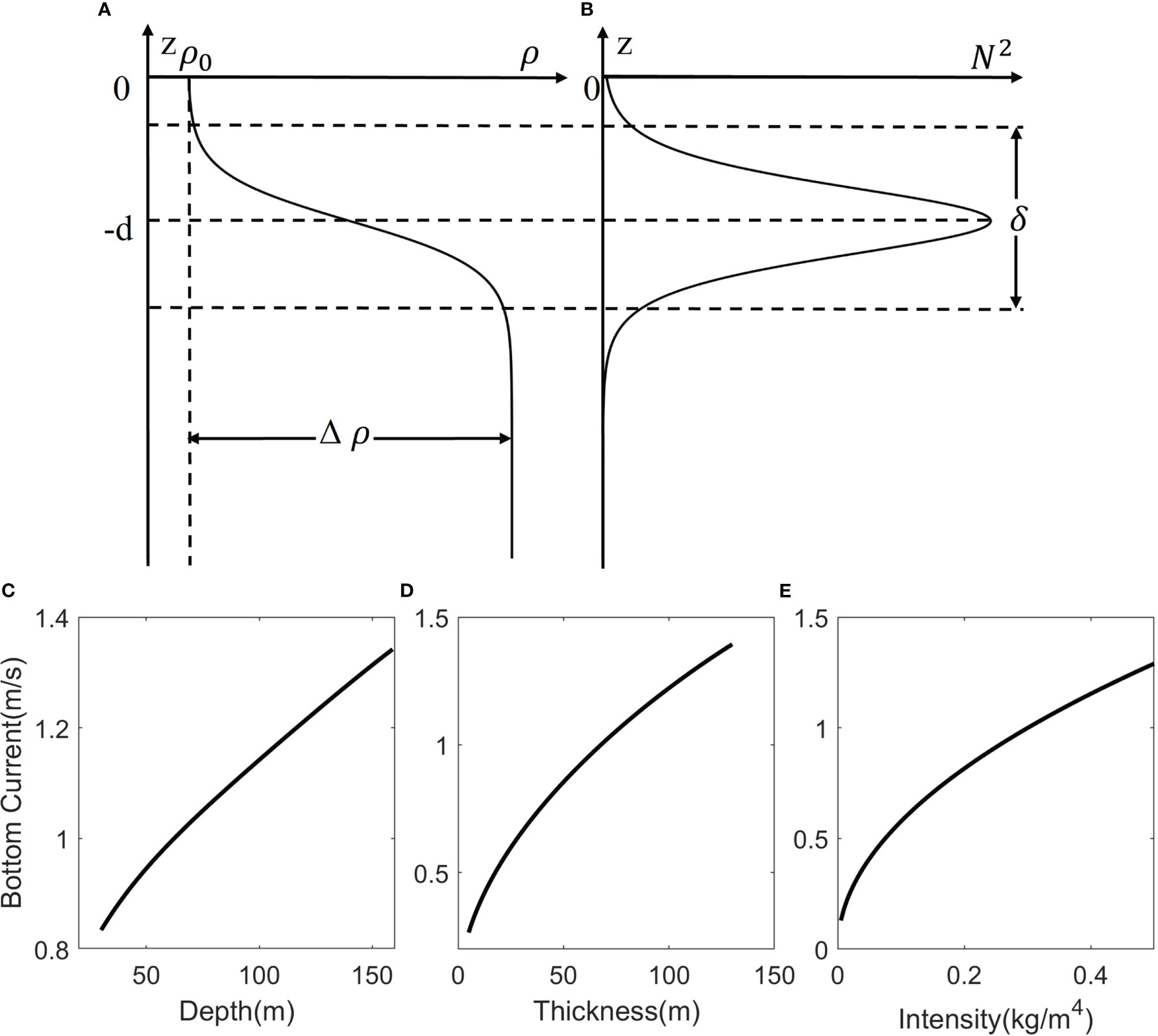
Figure 8 (A) Ideal vertical profiles of the density and (B) buoyancy frequency and calculated variations of the bottom current generated by an ISW with an amplitude of 100 m vs. the (C) depth, (D) thickness, and (E) intensity of the density pycnocline.

To clarify the effects of ocean stratification on the bottom current induced by ISWs, we calculate the bottom current under different stratifications through the KdV theory described in section 2.3. The density stratification profile can be approximately described by hyperbolic tangent function according to the mooring data (Wang, 2006):

$\begin{array}{ll}\rho (z)={\rho }_{0}exp\left\{\frac{\Delta \rho }{2{\rho }_0}tanh\left(\frac{-2(z+d)}{\delta }\right)\right\}& (24)\end{array}$

where ${\rho }_0$ is the sea surface water density, $\Delta \rho$ is the density difference between the upper and lower bounds of the pycnocline, $d$ is the pycnocline depth, and $\delta$ is the pycnocline thickness. The corresponding buoyancy frequency is given by the following:

$\begin{array}{ll}{N}^2(z)=-\frac{g}{\rho }\frac{d\rho }{dz}=\frac{g\Delta \rho }{\delta {\rho }_0}sec{h}^2\left(\frac{2(z+d)}{\delta }\right)& (25)\end{array}$

One can see that three parameters, $\Delta \rho$, d, and $\delta ,$ determine the density stratification profile as shown in Figures 8A, B. We calculate bottom currents induced by ISWs with an amplitude of 100 m that varies with the depth, thickness, and intensity of the pycnocline by the variable method. The results are shown in Figures 8C–E. One can see that as the pycnocline depth becomes deeper, the pycnocline becomes thicker, the pycnocline intensity increases, and the bottom current strengthens, implying that a deeper, thicker, and stronger pycnocline is a favorable condition for the generation of a stronger bottom current induced by ISWs. In winter, the pycnocline is deeper and thicker, so that the bottom current induced by ISWs becomes stronger.

According to the KdV theory, we calculate bottom currents induced by the ISWs in the northern SCS based on the monthly stratification data of the World Ocean Atlas (WOA). Figure 9 shows the distribution of bottom currents induced by ISWs with an amplitude of 100 m in the northern SCS. One can see that on the northern SCS continental slope, the ISW-induced bottom current is strongest in January (Figure 9A), followed by July (Figure 9C) and October (Figure 9D), and weakest in April (Figure 9B). This is consistent with the results calculated from the measured data, further illustrating that a deeper and thicker pycnocline is more likely to generate stronger bottom currents induced by ISWs in winter. In addition, the water depth is also an important factor affecting the intensity of bottom currents induced by ISWs. As shown in Figure 9, on the shallow continental slope, bottom currents are strong and gradually weaken as the depth becomes deeper.

FIGURE 9

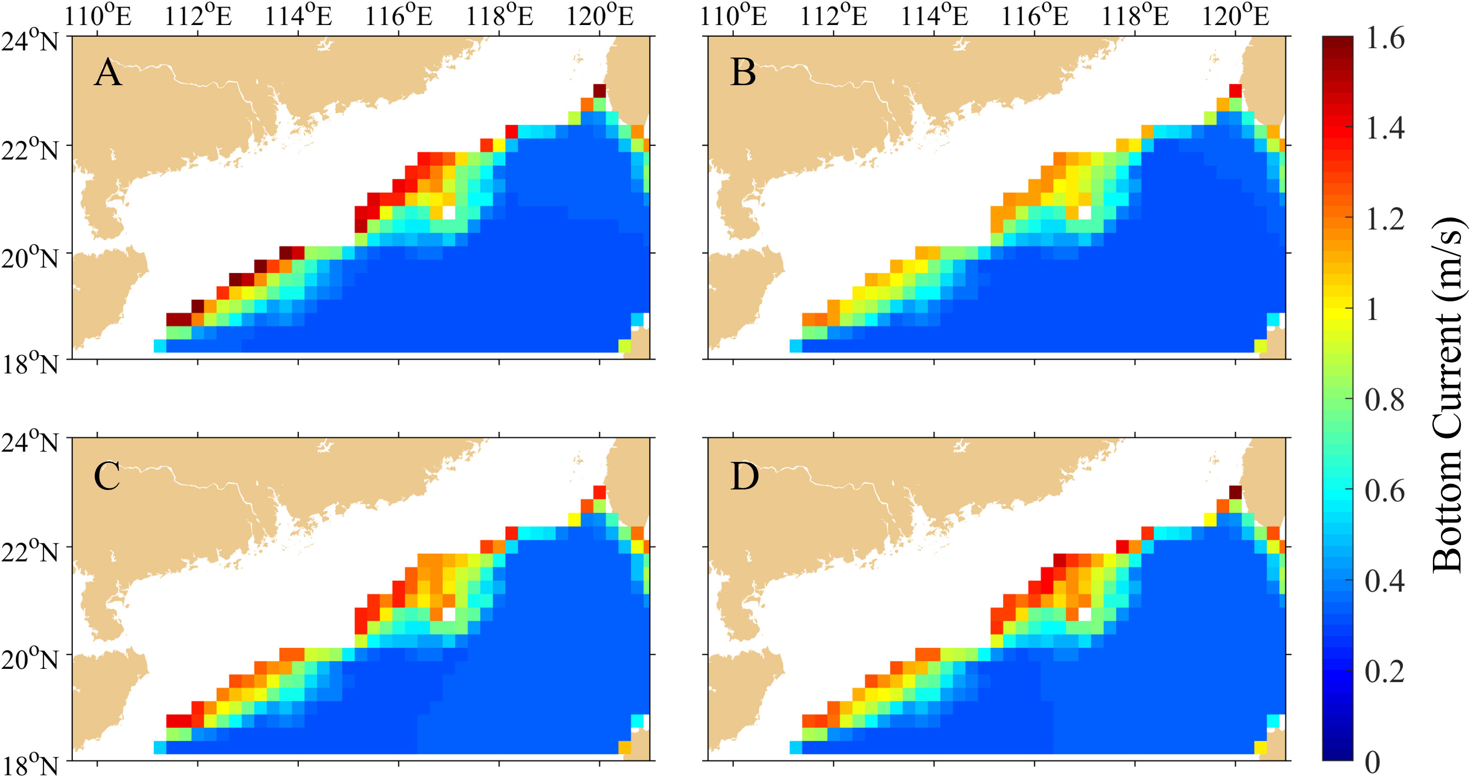
Figure 9 Distributions of bottom currents induced by the ISWs with the amplitude of 100 m in the northern SCS calculated from the WOA data. (A) January, (B) April, (C) July, and (D) October.

To further confirm the intrinsic links of the bottom current to the ISWs, we plot the relation of the bottom current velocity vs. the ISW amplitude using mooring-observed data. The result is shown in Figure 10, in which the theoretical curve is derived from the ISW current velocity solution of the KdV equation, Eq. 23, i.e.,

FIGURE 10

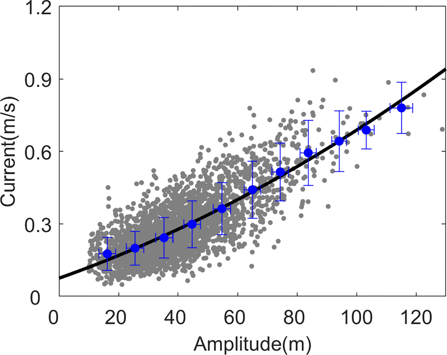
Figure 10 ISW-induced bottom current versus ISW amplitude. Gray dots are the mooring-observed data. The black line represents the KdV equation solution. Blue dots with standard deviation bars are the segment average values of the gray dots in a 10-m spacing of the amplitude from 10 to 130 m.

$\begin{array}{ll}{V}_{b, max}=k{\eta }_0·C_n=a_1{\eta }_0^2+a_2{\eta }_0+a_3& (26)\end{array}$

where ${\eta }_o$ is the ISW amplitude, $a_1=k\left|\alpha \right|/3$, $a_2=kc$, and parameters c, $\alpha ,$ and $\beta$ are determined by Eqs. 14a–c using mooring data. The values of the parameters are listed in Table 1. One can see that the ISW current velocity solution of the KdV equation fits the mooring data very well with $R^2=0.9915$, implying intrinsic links of the observed bottom current to the ISW amplitude. Particularly, when ${\eta }_0=0$, the ISW disappears, $a_3$ equals 0.077 $\text{m}/\text{s}$, which is defined as the background bottom current in this study.

TABLE 1

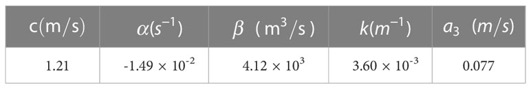
Table 1 Parameters in Eq. 26.

3.3 Seasonal variation of background bottom current

With the above method, we analyze the monthly ISW observation data as shown in Figure 11. From the fitting curves, monthly mean background bottom currents are obtained as shown as orange histogram in Figure 12. One can see that the taller background bottom current bars are distributed from December to April of the following year with a maximum value of 0.13 m/s in February and that the shorter bars are distributed from June to November with a minimum value of 0.03 m/s in October.

FIGURE 11

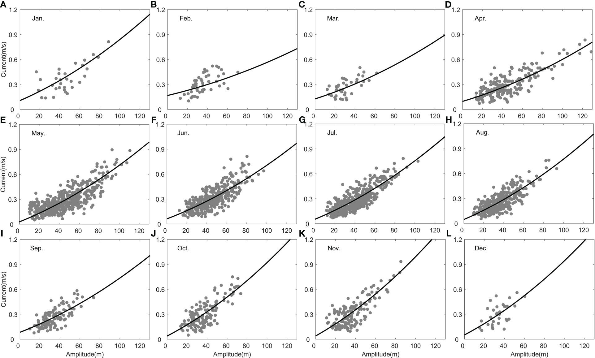
Figure 11 Monthly distribution of ISW-induced bottom current versus ISW amplitude (A–L). Gray dots are the mooring-observed data. Black lines represent the KdV equation solutions.

FIGURE 12

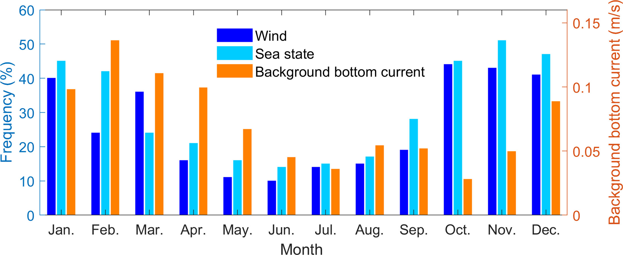
Figure 12 Comparisons of monthly background bottom currents with mean wind frequency (wind speed higher than 10 m/s) and sea state frequency (wave height higher than 2 m).

To explore the response of monthly background bottom currents to the sea surface processes, the histograms of the mean frequency of high wind conditions and high sea state conditions (Zheng et al., 2007) are shown in Figure 12. The correlation coefficients of the monthly background bottom currents with high wind condition and high sea state condition are 0.1402 and 0.2157, respectively, indicating that the seasonal variation of background bottom currents has no direct relationship with the sea surface processes.

On the other hand, previous investigations have revealed that the SCS is featured by active mesoscale eddies (Zheng, 2017). Zhang et al. (2022) further divided mesoscale eddies on the northern SCS shelf into four types: along-the-isobath type, intrusion-of-continental-shelf type, local wandering type, and shelf-internal-generation type, with a seasonal resolution. Thus, it is important to clarify the response of background bottom current to the behavior of concurrent mesoscale eddies. For this purpose, seasonal mean background bottom currents are calculated by the above method. As shown in Figure 13A, the background bottom current has obvious seasonal variations: strongest in winter, followed by spring, and weak in summer and autumn. Mesoscale eddy data are cited from Zhang et al. (2022).

FIGURE 13

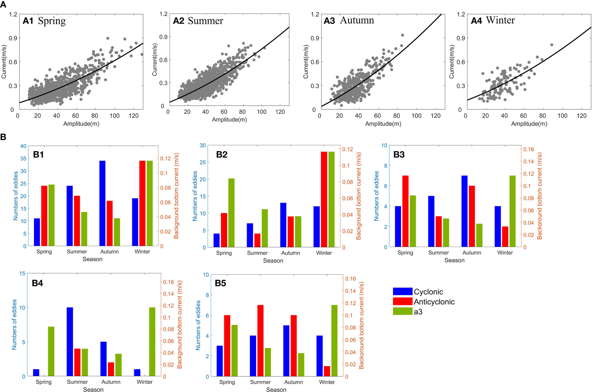
Figure 13 (A) Seasonal distribution (A1–A4) of ISW-induced bottom current versus ISW amplitude. Gray dots are the mooring-observed data. Black lines represent the KdV equation solutions. (B) Statistical histograms of seasonal variations of background bottom current velocity with the numbers of (B1) total mesoscale eddies, (B2) along-the-isobath-type mesoscale eddies, (B3) intrusion-of-continental-shelf-type mesoscale eddies, (B4) local wandering-type mesoscale eddies, and (B5) shelf-internal-generation-type mesoscale eddies.

Figure 13B shows comparisons of seasonal variation histograms of background bottom current velocity to numbers of concurrent mesoscale eddies. The correlation coefficients are listed in Table 2. One can see that there is the highest positive correlation between the background bottom current and the total number of anticyclonic mesoscale eddies with a correlation coefficient of 0.9721. The correlation coefficients with four types of mesoscale eddies defined by Zhang et al. (2022) vary from -0.024 to 0.8745 with 75% higher than 0.76. These results indicate that the seasonal variation of background bottom currents on the northern SCS continental slope is closely linked with the behavior of mesoscale eddies. This phenomenon is worth pursuing in future efforts.

TABLE 2

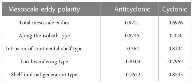
Table 2 Correlation coefficients of background bottom current (a3) to the number of mesoscale eddies.

4 Conclusions

A mooring was deployed on the northern SCS continental shelf to measure the current velocity, temperature, and salinity from 1 April 2020 to 6 November 2021. The mooring system was innovatively designed to focus on the measurement of the bottom current velocity from 0.5 to 5 m above the seafloor. The mooring data are used to figure out the dynamic mechanisms for occurrence of the strong bottom currents. The major findings are summarized as follows.

The statistical analysis results of mooring-observed current velocity data reveal that bottom currents in the study area are characterized by occurrence year-round with the seasonal variation and the velocity amplitudes up to O(50–90) cm/s, which are of the same order of the SCS western boundary current velocity (He, 2019). The spectral analysis results indicate that the currents induced by the internal tides and the ISWs comprise the dominant constituents of bottom currents.

The amplitude of the internal tide-induced bottom current constituent reaches 50 cm/s. In the total horizontal kinetic energy of the bottom current, the internal tides account for 52% on average and up to the highest 76% in January. The diurnal internal tide is the dominant component with an average proportion of 81%, and the semidiurnal internal tide occupies a proportion of 19%. The coherent internal tide dominates with an average proportion of 63%, while the incoherent internal tide accounts for 37%. In the semidiurnal internal tide, the incoherent component accounts for 47%, indicating that nearly half of semidiurnal internal tides is transmitted from other sea areas.

The bottom current component induced by the ISWs appears in the form of pulsating currents with the seasonal variation. The maximum current velocity amplitude up to 93 cm/s appears in November and exceeds 50 cm/s in all other months. The strength of the bottom current induced by ISWs has intrinsic links with the ISW amplitude, following the soliton propagation speed solution of the KdV equation. The bottom currents induced by the ISWs in the northern SCS calculated from the monthly stratification data of the WOA show that the strongest currents are distributed on the continental slope in winter.

Monthly and seasonal variations of background bottom currents are derived from the observation data of the ISW amplitudes. They are strongest in winter, followed by spring, and weak in summer and autumn. The results of the correlation analysis show that the seasonal variations of background bottom currents on the northern SCS continental shelf are closely correlated with the behavior of mesoscale eddies. This phenomenon is worth pursuing in future efforts.

Data availability statement

The raw data supporting the conclusions of this article will be made available by the authors, without undue reservation.

Author contributions

LC performed the experiment, data analyses and wrote the manuscript; XX contributed to the conception of the experiment; QZ contributed to the conception of the study; LR helped perform the analysis with constructive discussions; YW helped perform the experiment and analysis; QG helped perform the experiment and analysis. All authors contributed to the article and approved the submitted version.

Acknowledgments

This work was supported by the National Science and Technology Major Project (2016ZX05057015). WOA data are downloaded from https://www.nodc.noaa.gov/cgi-bin/OC5/woa13/woa13.pl.

Conflict of interest

The authors declare that the research was conducted in the absence of any commercial or financial relationships that could be construed as a potential conflict of interest.

Publisher’s note

All claims expressed in this article are solely those of the authors and do not necessarily represent those of their affiliated organizations, or those of the publisher, the editors and the reviewers. Any product that may be evaluated in this article, or claim that may be made by its manufacturer, is not guaranteed or endorsed by the publisher.

References

Alford M. H., MacKinnon J. A., Nash J. D., Buijsman M. C., Centuroni L. R., Chao S. Y., et al. (2015). The formation and fate of internal waves in the south China Sea. Nature 521 (7550), 65–69. doi: 10.1038/nature14399

PubMed Abstract | CrossRef Full Text | Google Scholar

Baines P. G. (1982). On internal tide generation models. Deep. Sea. Res. Part A. Oceanographic. Res. Papers. 29 (3), 307–338. doi: 10.1016/0198-0149(82)90098-X

CrossRef Full Text | Google Scholar

Butman B., Noble M., Folger D. W. (1979). Long-term observations of bottom current and bottom sediment movement on the mid-Atlantic continental shelf. J. Geophys. Res. 84 (C3), 1187–1205. doi: 10.1029/JC084iC03p01187

CrossRef Full Text | Google Scholar

Chen H., Xie X., Zhang W., Shu Y., Wang D., Vandomp T., et al. (2016). Deep-water sedimentary systems and their relationship with bottom currents at the intersection of xisha trough and northwest sub-basin, south China Sea. Mar. Geol. 378, 101–113. doi: 10.1016/j.margeo.2015.11.002

CrossRef Full Text | Google Scholar

Chen L., Zheng Q., Xiong X., Yuan Y., Xie H. (2018). A new type of internal solitary waves with a re-appearance period of 23 h observed in the south China Sea. Acta Oceanol. Sin. 37 (9), 116–118. doi: 10.1007/s13131-018-1252-y

CrossRef Full Text | Google Scholar

Chen L., Zheng Q., Xiong X., Yuan Y., Xie H., Guo Y., et al. (2019). Dynamic and statistical features of internal solitary waves on the continental slope in the northern south China Sea derived from mooring observations. J. Geophys. Res. Oceans. 124 (6), 4078–4097. doi: 10.1029/2018JC014843

CrossRef Full Text | Google Scholar

Connolly T. P., Mcgill P. R., Henthorn R. G., Burrier D. A., Michaud C. (2020). Near-bottom currents at station m in the abyssal northeast pacific. Deep. Sea. Res. Part II Topical. Stud. Oceanogr. 173, 104743. doi: 10.1016/j.dsr2.2020.104743

CrossRef Full Text | Google Scholar

Farmer D., Alford M., Lien R. C., Yang Y. J., Chang M. H., Li Q. (2011). From Luzon strait to dongsha plateau: stages in the life of an internal wave. Oceanography 24 (4), 64–77. doi: 10.5670/oceanog.2011.95

CrossRef Full Text | Google Scholar

Grimshaw R., Pelinovsky E., Talipova T., Kurkin A. (2004). Simulation of the transformation of internal solitary waves on oceanic shelves. J. Phys. Oceanogr. 34, 2774–2791. doi: 10.1175/JPO2652.1

CrossRef Full Text | Google Scholar

He Z., Lyu K., Quan Q. (2019). “The south China Sea western boundary current. chapter 4,” in Regional oceanography of the south China Sea. Ed. Hu, et al (London: World Scientific), 77–99.

Google Scholar

Holloway P., Pelinovsky E., Talipova T., Barnes B. (1997). A nonlinear model of internal tide transformation on the Australian north West shelf. J. Phys. Oceanogr. 27 (6), 871–896. doi: 10.1175/1520-0485(1997)027<0871:ANMOIT>2.0.CO;2

CrossRef Full Text | Google Scholar

Jackson C. (2007). Internal wave detection using the moderate resolution imaging spectroradiometer (MODIS). J. Geophys. Res. 112, C11012. doi: 10.1029/2007JC004220

CrossRef Full Text | Google Scholar

Jia Y., Tian Z., Shi X., Liu J. P., Chen J., Liu X., et al. (2019). Deep-sea sediment resuspension by internal solitary waves in the northern south China Sea. Sci. Rep. 9, 12137. doi: 10.1038/s41598-019-47886-y

PubMed Abstract | CrossRef Full Text | Google Scholar

Lan J., Wang Y., Cui F., Zhang N. (2015). Seasonal variation in the south China Sea deep circulation. J. Geophys. Res.: Oceans. 120, 1682–1690. doi: 10.1002/2014JC010413

CrossRef Full Text | Google Scholar

Lan J., Zhang N., Wang Y. (2013). On the dynamics of the south China Sea deep circulation. J. Geophys. Res.: Oceans. 118 (3), 1206–1210. doi: 10.1002/jgrc.20104

CrossRef Full Text | Google Scholar

Li L., Qu T. (2006). Thermohaline circulation in the deep south China Sea basin inferred from oxygen distributions. J. Geophys. Res.: Oceans. 111, C05017. doi: 10.1029/2005JC003164

CrossRef Full Text | Google Scholar

Li D., Wei Z., Wang Y., Li S., Xu T., Wang G., et al. (2019). Characteristics and temporal variations of near-bottom currents near the dongsha island in the northern south China Sea. Acta Oceanol. Sin. 38 (4), 80–89. doi: 10.1007/s13131-019-1415-5

CrossRef Full Text | Google Scholar

Lei S., Li X., Geng J., Xiong P., Yong Chang L., Pei Jun Q., et al. (2007). Deep water bottom current deposition in the northern South China Sea. Sci. China Ser. D.: Earth Sci. 50 (7): 1060–1066.

Google Scholar

Liu J., Cai S., Wang S. (2011). Observations of strong near-bottom current after the passage of typhoon pabuk in the south China Sea. J. Mar. Syst. 87 (1), 102–108. doi: 10.1016/j.jmarsys.2011.02.023

CrossRef Full Text | Google Scholar

Park J. H., Watts D. R. (2006). Internal tides in the southwestern Japan/East Sea. J. Phys. Oceanogr. 36 (1), 22–34. doi: 10.1175/JPO2846.1

CrossRef Full Text | Google Scholar

Pawlowicz R., Beardsley B., Lentz S. (2002). Classical tidal harmonic analysis including error estimates in MATLAB using T_TIDE. Comput. Geosci. 28 (8), 929–937. doi: 10.1016/S0098-3004(02)00013-4

CrossRef Full Text | Google Scholar

Pelinovsky E. N., Slunyaev A. V., Polukhina O. E., Talipova T. G. (2007). “Internal solitary waves,” in Solitary waves in fluids. Ed. Grimshaw R. (Southampton, Boston: WIT Press), 85–110.

Google Scholar

Shang X., Liu Q., Xie X., Chen G., Chen R. (2015). Characteristics and seasonal variability of internal tides in the southern south China Sea. Deep. Sea. Res. Part I. Oceanographic. Res. Papers. 98, 43–52. doi: 10.1016/j.dsr.2014.12.005

CrossRef Full Text | Google Scholar

Simmons H., Chang M. H., Chang Y. T., Chao S. Y., Fringer O., Jackson C., et al. (2011). Modeling and prediction of internal waves in the south China Sea. Oceanography 24 (4), 88–99. doi: 10.5670/oceanog.2011.97

CrossRef Full Text | Google Scholar

van Haren H. (2004). Incoherent internal tidal currents in the deep ocean. Ocean Dyn. 54, 66–76. doi: 10.1007/s10236-003-0083-2

CrossRef Full Text | Google Scholar

van Haren H. (2003). On the polarization of oscillatory currents in the bay of Biscay. J. Geophys. Res. 108 (C9), 3290. doi: 10.1029/2002JC001736

CrossRef Full Text | Google Scholar

Wang G. (2006). Numerical modelling on the generation process of the tidal internal waves over the northwestern south China Sea shelf (in Chinese) (Qingdao: Institute of Oceanology, Chinese Academy of Sciences).

Google Scholar

Wang J., Huang W., Yang J., Zhang H., Zheng G. (2012). Study of the propagation direction of the IWs in the south China Sea using satellite images. Acta Oceanol. Sin. 32 (5), 42–50. doi: 10.1007/s13131-013-0312-6

CrossRef Full Text | Google Scholar

Wang G., Xie S., Qu T., Rui X. H. (2011). Deep south China Sea circulation. Geophys. Res. Lett. 38, L05601. doi: 10.1029/2010GL046626

CrossRef Full Text | Google Scholar

Wu L., Xiong X., Li X., Shi M., Guo Y., Chen L. (2016). Bottom currents observed in and around a submarine valley on the continental slope of the northern south China Sea. J. Ocea. Univ. China 15 (6), 947–957. doi: 10.1007/s11802-016-3054-1

CrossRef Full Text | Google Scholar

Xie X., Shang X., van Haren H., Chen G. (2013). Observations of enhanced nonlinear instability in the surface reflection of internal tides. Geophys. Res. Lett. 40 (8), 1 580–1 586. doi: 10.1002/grl.50322

CrossRef Full Text | Google Scholar

Zhang T., Li J., Xie L., Zheng Q. (2022). Statistical analysis of mesoscale eddies entering the continental shelf of the northern south China Sea. J. Mar. Sci. Eng. 10 (2), 206. doi: 10.3390/jmse10020206

CrossRef Full Text | Google Scholar

Zhao Z. (2014). Internal tide radiation from the Luzon strait. J. Geophys. Res. Oceans. 119, 5434–5448. doi: 10.1002/2014JC010014

CrossRef Full Text | Google Scholar

Zhao Z., Klemas V., Zheng Q., Yan X. (2004). Remote sensing evidence for baroclinic tide origin of internal solitary waves in the northeastern south China Sea. Geophys. Res. Lett. 31, L06302. doi: 10.1029/2003GL019077

CrossRef Full Text | Google Scholar

Zheng Q. (2017). Satellite SAR detection of sub-mesoscale ocean dynamic processes (London: World Scientific), 151–169.

Google Scholar

Zheng Q., Susanto R. D., Ho C. R., Song Y. T., Xu Q. (2007). Statistical and dynamical analyses of generation mechanisms of solitary IWs in the northern south China Sea. J. Geophys. Res.: Oceans. 112, C03021. doi: 10.1029/2006JC003551

CrossRef Full Text | Google Scholar

Zheng Q., Xie L., Xiong X., Hu X., Chen L. (2020). Progress in research of submesoscale processes in the south China Sea. Acta Oceanol. Sin. 39 (1), 1–13. doi: 10.1007/s13131-019-1521-4

CrossRef Full Text | Google Scholar

Zheng Q., Xie L., Zheng Z. W., Hu J. (2017). Progress in research of mesoscale eddies in the south China Sea. Adv. Mar. Sci. (in Chinese). 35 (2), 131–158. doi: 10.1007/s13131-019-1521-4

CrossRef Full Text | Google Scholar

Zheng H., Yan P. (2012). Deep-water bottom current research in the northern south China Sea. Mar. Georesour. Geotechnol. 30 (2), 122–129. doi: 10.1080/1064119X.2011.586015

CrossRef Full Text | Google Scholar

Zhu Y., Liang X. (2020). Coupling of the surface and near-bottom currents in the gulf of Mexico. J. Geophys. Res.: Oceans. 125, e2020JC016488. doi: 10.1029/2020JC016488

PubMed Abstract | CrossRef Full Text | Google Scholar

Zu T., Gan J. P., Erofeeva S. Y. (2008). Numerical study of the tide and tidal dynamics in the south China Sea. Deep. Sea. Res. Part I.: Oceanographic. Res. Papers. 55 (2), 137–154. doi: 10.1016/j.dsr.2007.10.007

CrossRef Full Text | Google Scholar