 Jianfeng Tong
 Weiqi Wang1
 Zhenhong Zhu
 Siqian Tian
95% of researchers rate our articles as excellent or good
Learn more about the work of our research integrity team to safeguard the quality of each article we publish.
Find out more
ORIGINAL RESEARCH article
Front. Mar. Sci. , 05 June 2023
Sec. Marine Fisheries, Aquaculture and Living Resources
Volume 10 - 2023 | https://doi.org/10.3389/fmars.2023.1162064
This article is part of the Research Topic Deep Learning for Marine Science View all 40 articles
Nowadays, most fishing vessels are equipped with high-resolution commercial echo sounders. However, many instruments cannot be calibrated and missing data occur frequently. These problems impede the collection of acoustic data by commercial fishing vessels, which are necessary for species classification and stock assessment. In this study, an automatic detection and classification model for echo traces of the Pacific saury (Cololabis saira) was trained based on the algorithm YOLO v5m. The in situ measurement value of the Pacific saury was measured using single fish echo trace. Rapid calibration of the commercial echo sounder was achieved based on the living fish calibration method. According to the results, the maximum precision, recall, and average precision values of the trained model were 0.79, 0.68, and 0.71, respectively. The maximum F1 score of the model was 0.66 at a confidence level of 0.454. The living fish calibration offset values obtained at two sites in the field were 116.30 dB and 118.19 dB. The sphere calibration offset value obtained in the laboratory using the standard sphere method was 117.65 dB. The differences between in situ and laboratory calibrations were 1.35 dB and 0.54 dB, both of which were within the normal range.
As an important method for fishery resource surveys, hydroacoustic technology enables fast and independent testing, that is both harmless for the resources and accurate. Moreover, underwater acoustic spatial information with time series can be obtained (Foote and Rothschild, 2009; Haris et al., 2021). Hydroacoustic detection technology plays an important role in analyzing fish migration paths (Martignac et al., 2015; Gjøsæter et al., 2017), fish habitat distribution (Slotte et al., 2004; O'Donncha et al., 2021), and fish resource changes (Melvin et al., 2016; Aranis et al., 2022). It also allows to study zooplankton sound scattering layers (Boswell et al., 2020; Xue et al., 2021). The acoustic characteristics of a single organism or a biotic aggregate are defined as echo traces (Reid, 2000). The SHAPES theory (Coetzee, 2000) was published to provide a method of analyzing fish populations based on these echo traces. The main parameters the theory uses are the morphology and echo strength distribution of echo traces. Based on the above theory of fish echo trace analysis, the distributions of adult and juvenile sardine aggregation were found to be significantly different in the Mediterranean region (Tsagarakis et al., 2012). Swarms of anchovy (Engraulis ringens), common sardine (Sardinops sagax), and Pacific jack mackerel (Trachurus symmetricus) were identified by the SHAPES theory in northern and south-central Chilean waters. This analysis innovatively uses a statistical model to automate the classification of large quantities of fish echo traces (Robotham et al., 2010). The above studies demonstrate the feasibility of distinguishing species and age groups by features of fish school echo traces. However, the echo traces that emerge in response to discrete single fish situated around the school were often ignored. The echo traces of discrete individuals are usually inverted ‘V’-shaped or lightning-shaped (Reid, 2000). In previous studies (Boyra et al., 2019; Julie et al., 2020; Khodabandeloo et al., 2021), single fish echo traces were the main data source for measuring the in situ target strength values of different fish species. These single fish echo traces are important for fish species classification. Different fish species (Sawada et al., 2009), swimming tilt angles (Fernandes et al., 2016; Tong et al., 2022), swimming speeds (Lee et al., 2010), and fish swim bladder sizes (Sobradillo et al., 2019) affect the magnitude of fish target strength values. Because of dense fish aggregation during fishing activities, there are numerous targets on the echogram, making the detection and extraction of single fish echo images more challenging because of interference of environmental and instrument noises. Thus, most current in situ target strength measurement applications still require rigorous equipment and environmental conditions, while having limited application scope for measured target strength values.
Previous studies predicted the categories of echo trace and large-scale automatic classification using the calculation power of computers. Initially, statistical models were used to classify morphological parameters of the acoustic image measurements and echo strength values (LeFeuvre et al., 2000). These models include supervised machine learning models, such as classification tree (Fernandes, 2009), random forest (Fallon et al., 2016), support vector machine (Robotham et al., 2010), as well as unsupervised machine learning models such as K-means (Ito et al., 2013), Gaussian mixture models (Robotham et al., 2010), and principal component analysis (Lawson et al., 2001). However, statistical models are dependent. Digital image processing techniques and related acoustic methods are required to capture and enhance the echo trace features and infer the variability between feature parameters to complete the automatic identification process. Basic hypotheses are established based on feature values and variability to guide model training, which increases the difficulty and time consumption of data processing.
Deep learning techniques have been employed to develop a number of available network frameworks (Wang et al., 2022; Wang et al., 2023a). These frameworks and the modules that are based on them have been widely applied for underwater image enhancement (Wang et al., 2023b; Wang et al., 2023c) and noise control (Wang et al., 2023d). Among them, convolutional neural network (CNN) is one of the more widely used network architectures. The advent of CNN has increased the freedom of machine self-learning (Rathi et al., 2017; Albawi et al., 2018; Gu et al., 2018) while providing more possibilities for the identification of fish echo traces. Currently, target detection algorithms based on CNN can be classified into two-stage algorithms represented by Faster R-CNN (Li et al., 2015) and one-stage algorithms represented by YOLO (You Only Look Once) (Jalal et al., 2020). The two-stage algorithms mainly include two stages of interest region extraction and image detection, and can achieve higher recognition accuracy than single-stage algorithms. The increased computational power obtained by the region of interest extraction stage also limits the speed with which the algorithm can detect the target. Compared with a two-stage algorithm, the YOLO algorithm-based single-stage algorithm implements target detection and bounding box regression operations directly on the image, thus achieving a higher target detection speed. However, its recognition accuracy is slightly lower than that of the two-stage algorithm model. In a recent study, a deep learning-based target detection algorithm was applied to the target detection of underwater fish optical images. Li et al. (2015) and Li et al. (2016) captured underwater acoustic images and achieved recognition of fish in images by the faster R-CNN algorithm. Wageeh et al. (Wageeh et al., 2021) used a YOLO model with the introduction of an image enhancement algorithm to achieve automatic detection and counting of fish at a fish farm. Wang et al. (Wang et al., 2021) established a basic line for underwater object detection based on the YOLO v5 algorithm, which facilitated subsequent research on the detection of underwater objects. Jalal et al. (Jalal et al., 2020) proposed a method for detecting and identifying fish in complex underwater environments by combining a Gaussian mixture model, an optical flow module to detect the temporal information of fish swimming in the video, and a YOLO target recognition module to improve the comprehensive accuracy of video target detection. Acoustic images are usually captured in the form of one-channel graphing, which contains less information than optical images, usually containing three channels. This is challenging for acoustic image recognition using the YOLO model. The YOLO model is still valid for small target echo target recognition in the presence of noise in acoustic images (Fang and Wang, 2021).
In this study, the acoustic data collected by commercial Pacific saury (Cololabis saira) fishing vessels were used as original dataset to train the YOLO model. The pre-processing module of the acoustic data was established using image processing. Based on the YOLO v5 algorithm, the automatic target detection model was constructed to complete the automatic detection and target identification of single fish and fish schools in the echograms. Finally, echo traces extracted from the target recognition were used to identify single fish and calibrate the echosounder of the commercial fishing vessel.
The fishing platform is the ocean-going Pacific saury fishing vessel FV ‘Ming Hua,’ with a total length of 73.98 m and a draft of 5 m. The vessel entered the fishing grounds on May 13, 2021, and carried out the fishing of Pacific saury and squid (Todarodes pacificus). In this study, the data collected at the time of catching Pacific saury were used as the original dataset. The main area of the Pacific saury is the high seas region of the northwest Pacific Ocean (41°–48° N, 166°–172° E) (Figure 1), using a stick-held dipnet for fishing. The acoustic instrument used for acoustic data collection was a Hondex HE-1500Di (The Honda Electronics Co., Ltd., Toyohashi, Japan) single-beam commercial echo sounder. The basic parameters of the echo sounder are shown in Table 1. The commercial echo sounder was modified to save the raw echo level data collected by the transducer directly and combine it with both GPS data and time series. Then, the data were stored on a flash memory card. The detecting depth of the echo sounder was 300 m, and each memory card could collect 6.8 h of acoustic data.
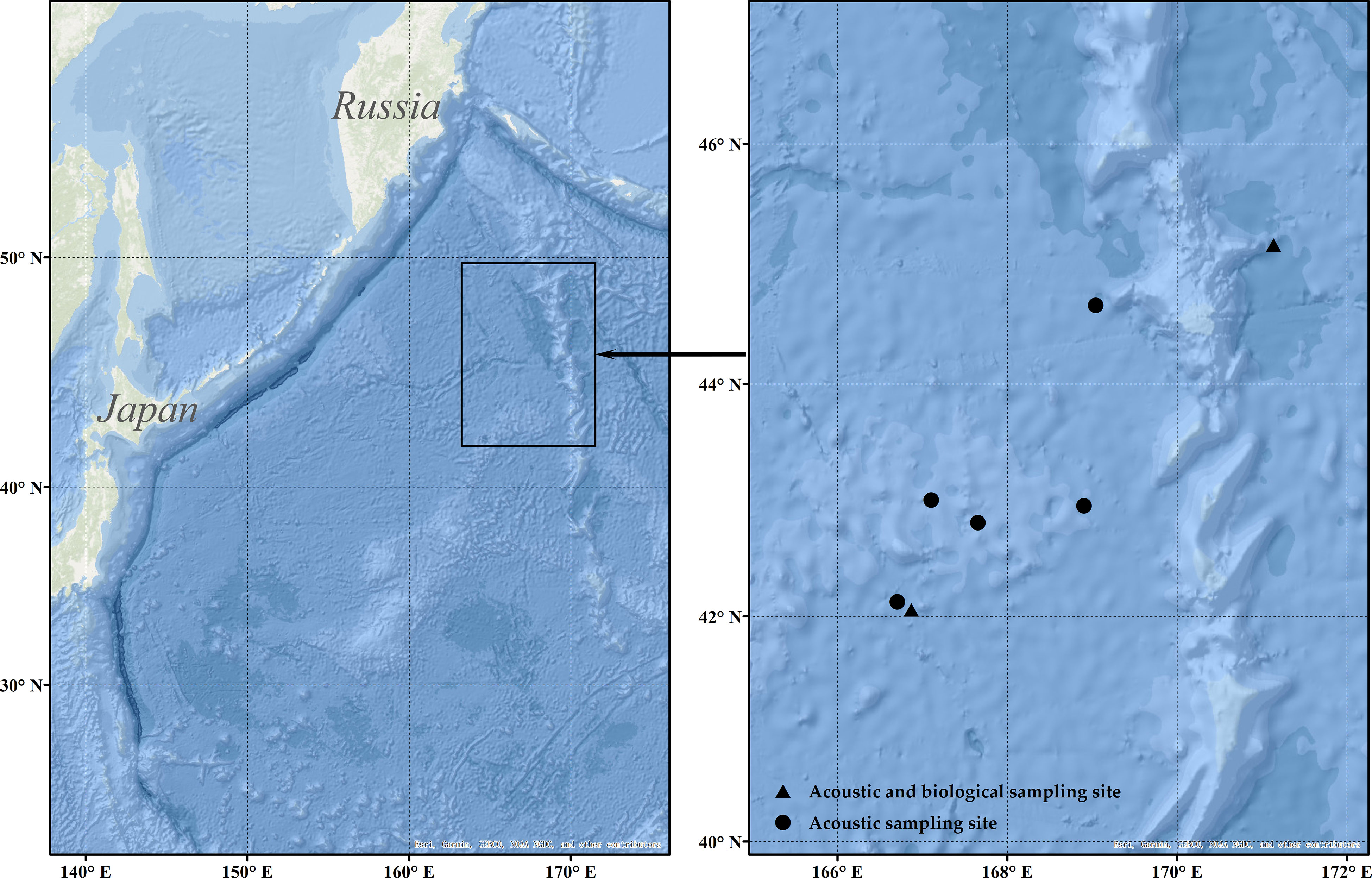
Figure 1 The black frame in the left figure panel indicates the range of acoustic monitoring; the black dots in the right figure panel indicate acoustic monitoring data sampling sites; the black triangles indicate acoustic and biological sampling sites.

Table 1 Main parameters of the Hondex HE-1500Di echo sounder.
The acoustic echograms obtained from the original acoustic dataset contain electromagnetic pulse noise from other fishing vessel equipment, environmental noise, and zooplankton reverberation. These noises can be a great obstacle for the identification and labeling of fish schools and single fish, as well as a challenge for learning single fish and fish school features during the model training process. In this study, an acoustic data pre-processing algorithm is proposed based on digital image processing technology to remove both noise and reverberation. The algorithm flow is shown in Figure 2.
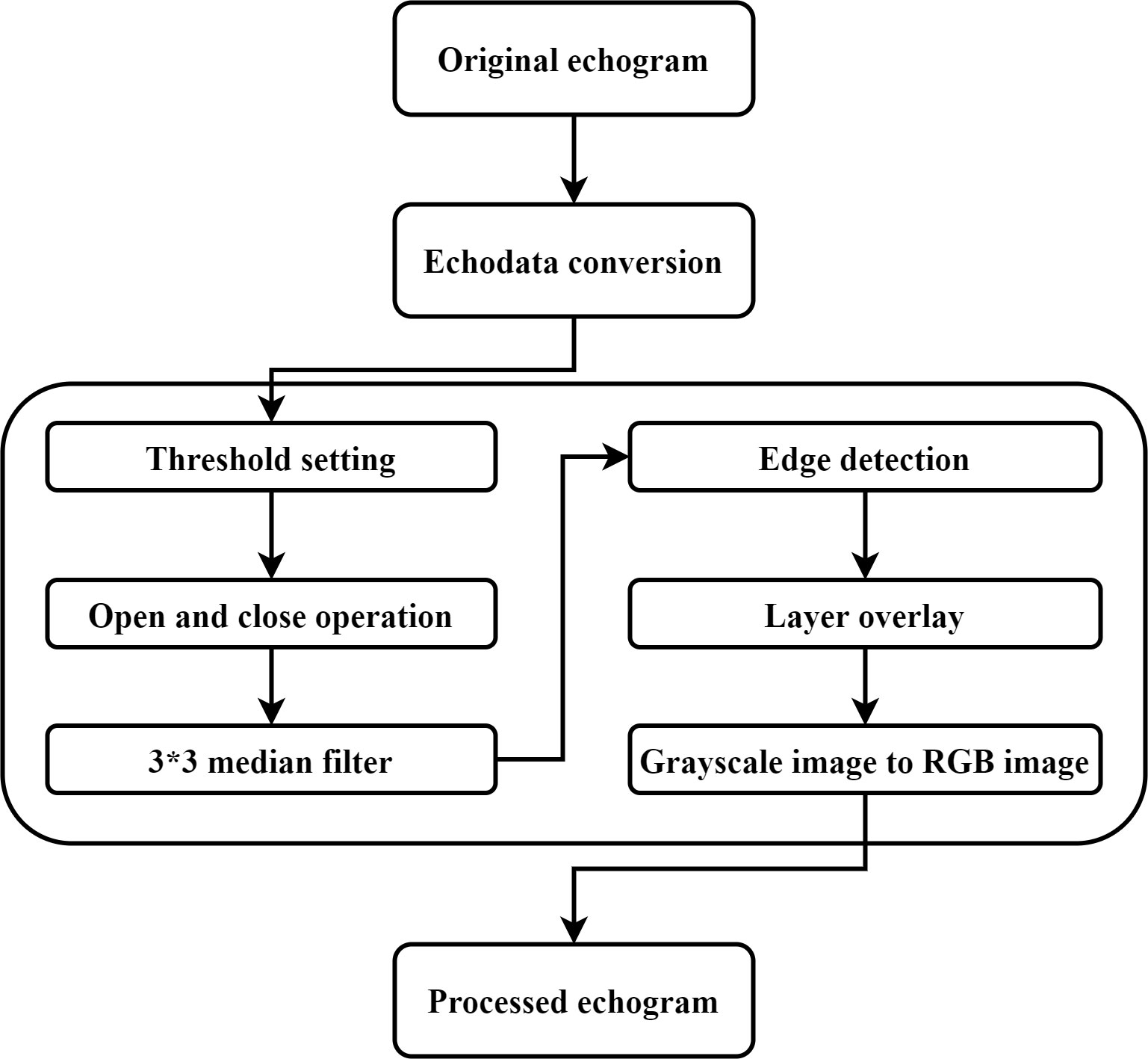
Figure 2 The architecture of the developed acoustic data pre-processing algorithm.
The echo level value in the acoustic data was first converted to sound backscattering strength values. The conversion formula is shown in Equation (1):
where is the received echo level (dB re 1 μV); is the sound absorption coefficient; is the depth value; is the equivalent beam angle; is the sound speed in water; and is the pulse length. is a transmitting and receiving factor, which is determined by the sphere calibration (dB) according to Equation (7). The data within 5 m of the sea surface of the acoustic data were removed according to the draft depth of the fishing vessel to avoid interference of the data by bubbles generated by the vessel and the movement of the surf. The integration threshold range of the acoustic data is set, and the part outside the integration threshold is removed to avoid the disturbance of the echo data by zooplankton and large predators. The integration threshold was set to range from 20 dB to 64 dB according to the integration settings in previous small pelagic fish resource surveys (Axenrot et al., 2004; Trumpickas et al., 2020). The small discrete noise generated by bubbles and the high-frequency impulse noise caused by instruments were removed using the open-close operation and the 3*3 median filter, respectively. The edge detection algorithm was used to detect the edge of the echo trace. The morphology, depth, and scattering strength of the echo trace are measured using the regionprops function. To prepare the echogram data for the process of target detection by YOLO v5, the grayscale image was transformed by the first-order numerical matrix. Each value in the matrix is mapped to the set colormap, the colors in the colormap are all RGB colors, and each color is a double float value in the interval [0,1]. The data of the matrix is normalized to correspond with the color value, and different values represent different colors. Thus, the indexed image using RGB color is formed. At this stage, the acoustic data preprocessing is complete. The specific process of pre-processing is detailed in Appendix A.
After pre-processing and morphological measurements, the echo traces that remained on the 50-kHz echograms were filtered. The location of the Pacific saury school was approximately determined by comparing the time of each catch in the fishing logbook for further filtering. The method of determining whether an echo trace is a single fish by analyzing the echo trace height related to pulse length has been applied to in situ target strength measurements (Didrikas and Hansson, 2004; Sawada et al., 1993). In this study, the above method was used to filter and separate single fish echo traces. The fish school was filtered with reference to the SHAPES algorithm (Coetzee, 2000). Echo traces with a height larger than 1 m and a length longer than 5 m were classified as fish schools. The remaining echo traces were classified as multiple fish. The three types of echo traces were labeled as “0” for single fish, “1” for multiple fish, and “2” for fish schools.
The YOLO v5 model is one of the representative models of one-stage target detection models based on deep learning. The four main versions in the existing YOLO v5 series are named YOLO v5s, YOLO v5m, YOLO v5l, and YOLO v5x. The differences between these four versions are the depth and width of the model network. Different network depths determine the number of convolutional layers, and different network widths determine the number of convolutional kernels in one convolutional layer. The network depth and width of these four versions of the model increase sequentially. An increase in the number of convolutional kernels and convolutional layers represents an enhancement in the recognition accuracy of the model, but also increases the size of model. To run the model on devices with low computing power while ensuring the detection accuracy, YOLO v5m was used as the base training model for the automatic detection experiments. YOLO v5m has a smaller model complexity compared to YOLO v5l and YOLO v5x, thus enabling model training on lower-computing devices. YOLO v5m also has a better small target detection capability compared to YOLO v5s. The main network structure of the model is shown in Figure 3. Its structure consists of four parts: Input, Backbone, Neck, and Prediction.
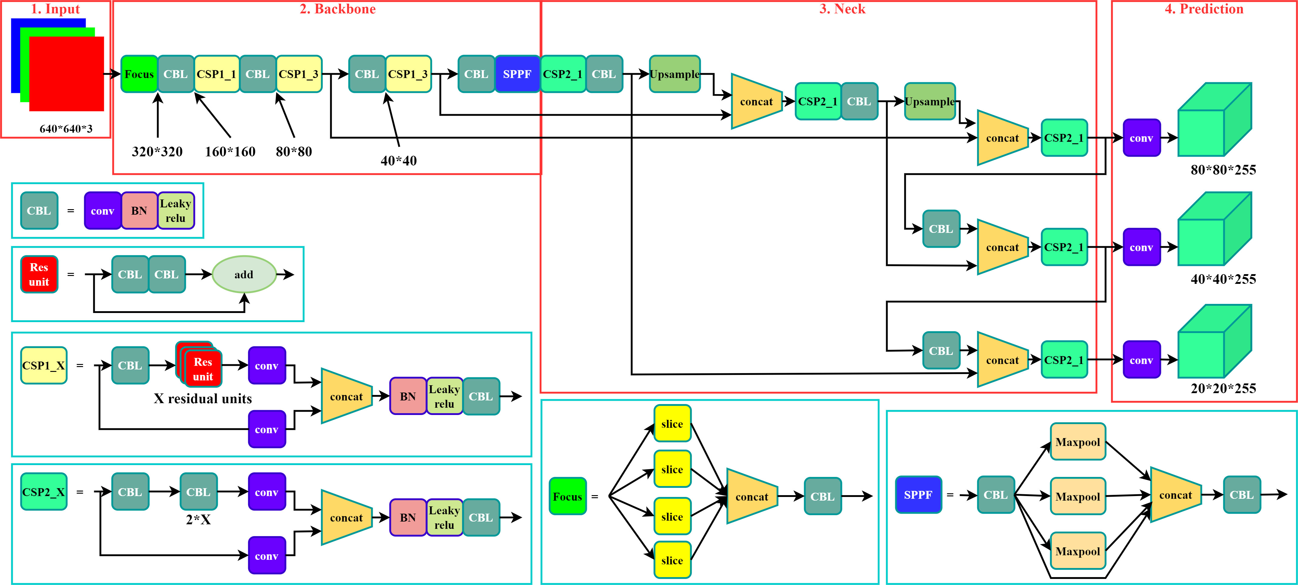
Figure 3 The main architecture of the YOLO v5m model.
The size of the imported RGB images in three channels set at the input side was 640 by 640 pixels When importing the images from the dataset into the model for training, the model automatically scaled the image size to the set size using the adaptive image scaling module. The Mosaic data enhancement algorithm and adaptive anchor frame calculation method were used at the input side to enhance the generalization ability of the model.
The backbone network part of the model mainly includes the four modules of focus, CBL, CSP, and SPPF. Among them, the focus module is used for downsampling, slicing, and convolution. Adjacent pixels in the image were first sampled using the down sampling and slicing method. After this operation, an image was divided into four feature maps, thus the number of channels is expanded four times without loss of information, and the size of the obtained feature maps was 320*320*12. Then, the image was convoluted by using convolutional kernel, and the final feature maps were also 320*320*32. Compared with common down sampling, the focus module completes image down sampling without loss of information. The CBL module contains convolution (conv), batch normalization (BN), and Leaky Relu, which serve to convolve the input data. The CSP module contains the CBL module and its components, with the addition of a residual component to avoid network degradation caused by gradient disappearance. The CSP module enables the model to learn more features. The SPPF module converts feature maps of arbitrary size into feature vectors of fixed size via the CBL module and maxpooling. The image was sliced and convolved into a 320*320*32 feature map by the focus module, convolved, and the residual features of the image were extracted by the CBL module. The number of network channels was expended through the SPPF module after earning the residual image features with the CSP module.
Model training was conducted using an Intel (R) Core (TM) i7-10875H CPU @ 2.30 GHz, GPU selected NVIDIA Geforce GTX1650 with 4 GB of video memory, using PyTorch 1.13 as the deep learning framework. The number of epochs was set to 300 in model training, and the batch size was set to 16.
Precision (P), recall (R), mean average precision (mAP), and F1-Score were used as indicators to evaluate the performance of the echo trace target detection model. P represents the precision and accuracy of the model, while R represents its recall and completeness. Formulas of P and R are shown in Equations (2) and (3):
where TP is truly positive, indicating that prediction and actual exist at the same time; FP is false positive, indicating that actually does not exist but prediction does; FN is a false negative, indicating that actual exists, but prediction does not. While mAP represents the average accuracy of all target categories detected by the model, the formula is obtained by averaging the average precision (AP) values of all targets. The F1-score represents the summed average of precision and recall with a maximum value of 1 and a minimum value of 0. This parameter allows for a more intuitive representation of the detection accuracy of the model. AP and mAP could be calculated using Equations (4) and (5):
where is the amount of change in recall and is the precision of the interpolation segment when the recall is . The F1-Score is calculated according to Equation (6):
When acoustic surveys are conducted using fishing vessels, the lack of sufficient time for standard process instrument calibration of echo sounder indicates the need to evaluate instrument performance using a simplified method. In previous studies, certain calibration methods using objects with known physical properties have been used to calibrate the echosounder, including the calibration sphere method (Knudsen, 2009), the natural seafloor calibration method (Eleftherakis et al., 2018), and the living fish calibration method (Johannesson and Losse, 1977). Of these, the natural seafloor calibration method and the living fish calibration method (both relative calibration methods) can test the performance of the echo sounder within a short period, and are thus suitable for the calibration of acoustic instruments on commercial fishing vessels. The acoustic data collected in this study were not detected at the sea bottom because the area is located in the deep sea. Hence, the living fish calibration method was used for commercial echo sounder calibration.
The instrument calibration of the commercial echo sounder was performed in a laboratory pool before the fishing vessel was put to sea. The sphere calibration offset was obtained in a standard sphere calibration process. The formula for sphere calibration offset is shown in Equation (7):
where is the distance between the target and transducer; is the hydroacoustic absorption coefficient; is the target strength of the calibration sphere; is the echo level (dB re 1μV) of the calibration sphere on the beam axis. The YOLO v5 model was used to detect single fish echo traces, and the max echo level values of the echo trace in the bounding box were extracted for calculating the on-axis measurement value () (dB). is calculated according to Equation (8):
where is the directivity of the transducer. This study used a single-beam transducer to measure the target echo level value. When the target is directly below the transducer, is 0, and the target echo level value reaches the maximum at this time. The prolate spheroidal model (PSM) was used to simulate the target strength of the Pacific saury, and the catches caught during the acoustic monitoring were sampled to obtain 100 fish from two sampling sites. The total length and fork length of the Pacific saury were measured on board. The correlation coefficient was calculated based on the swim bladder fish model, as shown in Equation (9):
where is defined as the absolute value of the backscattering amplitude from the fish in the far field region; is half of the fork length; is the length of the swim bladder, and is the fork length of the fish. For the ratio of the length of the swim bladder to the fork length of the fish in Equation (9), a typical value of 0.34 is assumed based on the research of Furukawa (Furusawa, 1988). The is calculated based on Equation (9), as shown in Equation (10):
The living fish calibration offset is obtained by subtracting the in situ from the , as shown in Equation (11):
The raw acoustic data were collected over 7 d of fishing. During the catching process, the number of Pacific sauries in the total catch was highest, which shows that when fishing with the collector light, the fish that rise to the sea surface are mainly saury; furthermore, the fish that are attracted by the beam emitted by the transducer are saury. An example original acoustic echogram obtained during the fishing process is shown in Figure 4. The fish gradually concentrated within the water layer about 30 m from the sea surface when the fish trap light was turned on. The echo data within 30 m intercepted from Figure 4 are shown in Figure 5, where Figure 5A shows the fish underwater during the search process. Figures 5B, C show the underwater fish when the fish trap light is turned on. The fish gradually gathered in the water layer around 20 m and formed a dense cluster. Figure 5D shows the fish underwater during the fishing process. The fish were mainly concentrated in the water layer of 20–30 m depth, while the fish within 20 m were relatively discrete. Many bubbles and noise signals were generated by the fishing vessel in the above images, and reverberant signals were generated by plankton, which is the main prey of the Pacific saury.

Figure 4 Example of an original acoustic echogram associated with Pacific saury during the search and catch period.
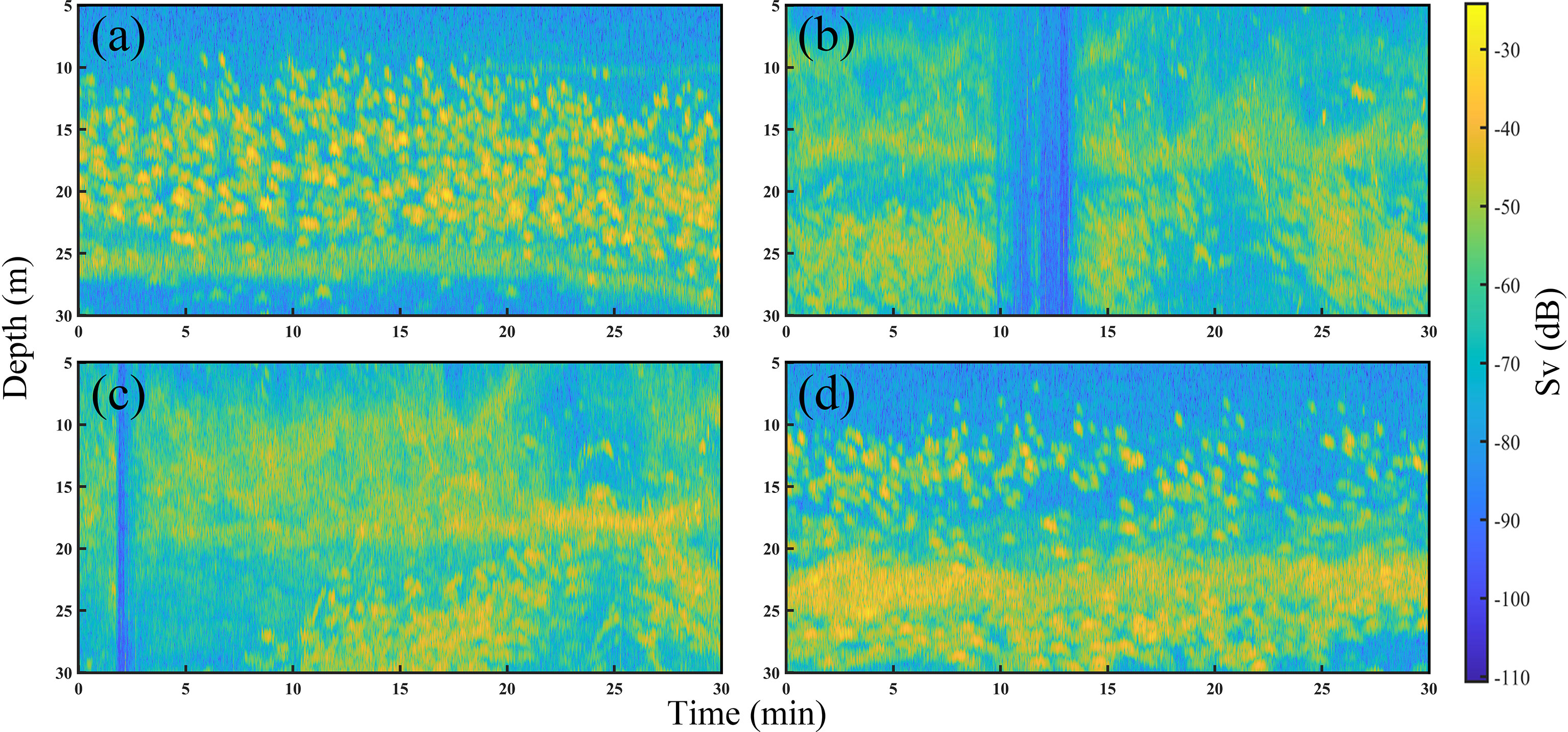
Figure 5 Acoustic echograms associated with Pacific saury in the surface layer (5–30 m) during the searching the catching periods. (A) The swarm during the searching process. (B) The swarm when the fish collector light was turned on. (C) The swarm after a period of illumination of the water surface by the collector light. (D) The swarm during the catching process.
The acoustic echogram after pre-processing using the algorithm and labeling is shown in Figure 6. The echograms of the echo trace of Pacific saury were separated, and the noise and reverberation generated by the plankton were removed. The depth and morphology of fish could be seen more clearly in the echograms. The isolated echo traces were boxed out using the red bounding box. The parameters obtained from the measurements were used to classify the echo trace as “0” for single fish, “1” for multiple fish, and “2” for schools. The labeled results are located in the upper left corner of the red bounding box.
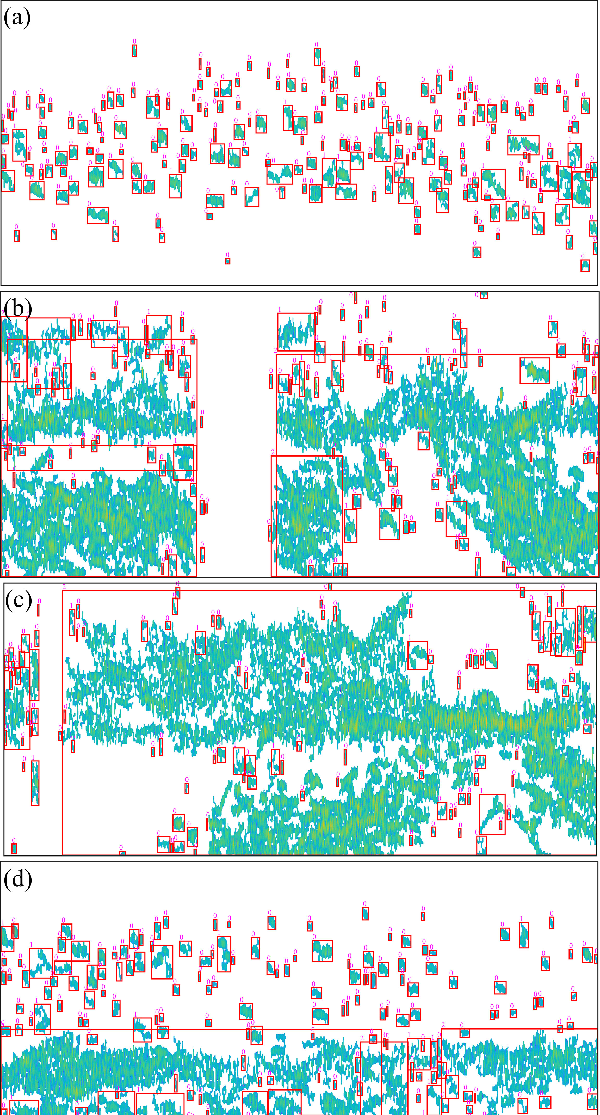
Figure 6 Results of echogram pre-processing and echo trace labeling. The figure panels of (A–D) correspond to the original echo images in Figure 5. The small pink numbers represent single fish (“0”), multiple fish (“1”), and fish groups (“2”).
The pre-processed echograms are used as automatic recognition model training dataset. The duration of each pre-processed echogram was 30 min, and the depth of the echogram was 30 m. According to the size of imported images (640*640*3), the resolution in the vertical direction was 4.6 cm and the resolution in the horizontal direction was 2.81 sec. Because the speed of the fishing vessel was not constant during the fishing process, the horizontal resolution of each data is different. See appendix B for details. A total of 91 echograms were finally available in the dataset. A total of 10,710 echo traces were extracted from the echograms, including 7,725 single-fish echo traces, 2,346 multiple-fish echo traces, and 639 echo traces of the school. The dataset was randomly divided into a training set (85%), a validation set (5%), and a test set (15%).
Table 2 presents the evaluation metrics of the observation used to test the effectiveness of the trained model. The recall of the model reached a maximum of 0.68 when the number of training epochs was 211. The precision and mAP_0.5 reached maximum values of 0.79 and 0.71, respectively, when the number of epochs was 281. The mAP_0.5:0.95 reached a maximum of 0.43 when the number of epochs was 300. The curve of the F1-score related to the confidence level is shown in Figure 7. The F1-score for all classes at a confidence level of 45.4% reached a maximum value of 0.66. At a confidence level of about 55%, the F1-score remained above 0.6, then decreased rapidly until it reached zero. The echograms from the test set were imported into the trained model. Detection results are shown in Figure 8.
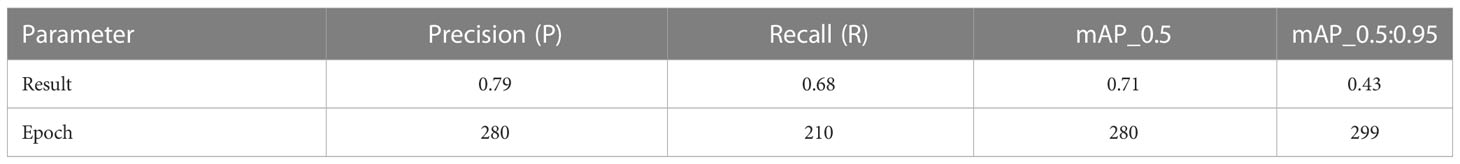
Table 2 The main results of model training.
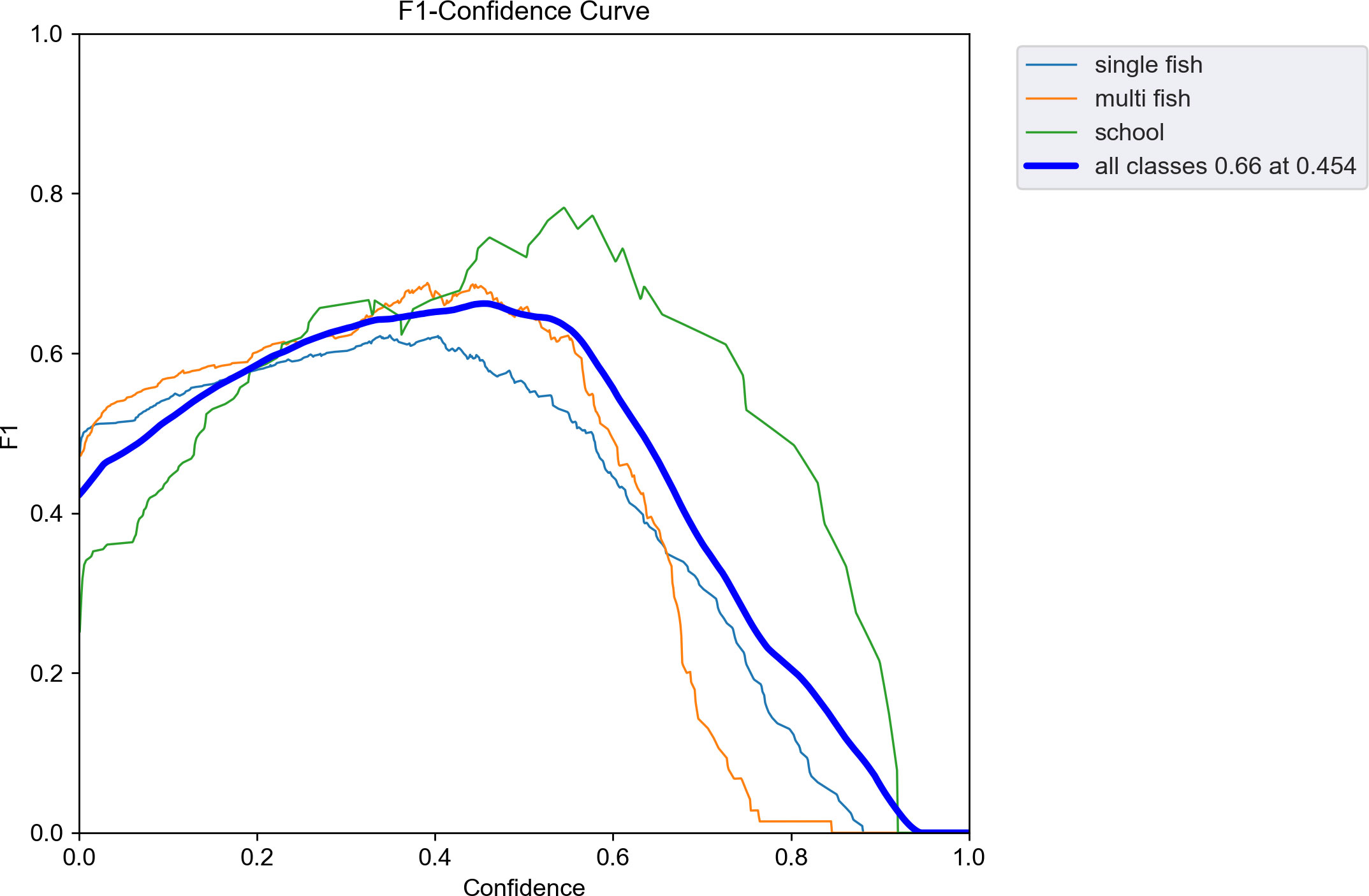
Figure 7 Curves of F1 scores related to the confidence level. The thinner three lines indicate the F1 scores for each class. The thick line indicates the F1 score for all classes.
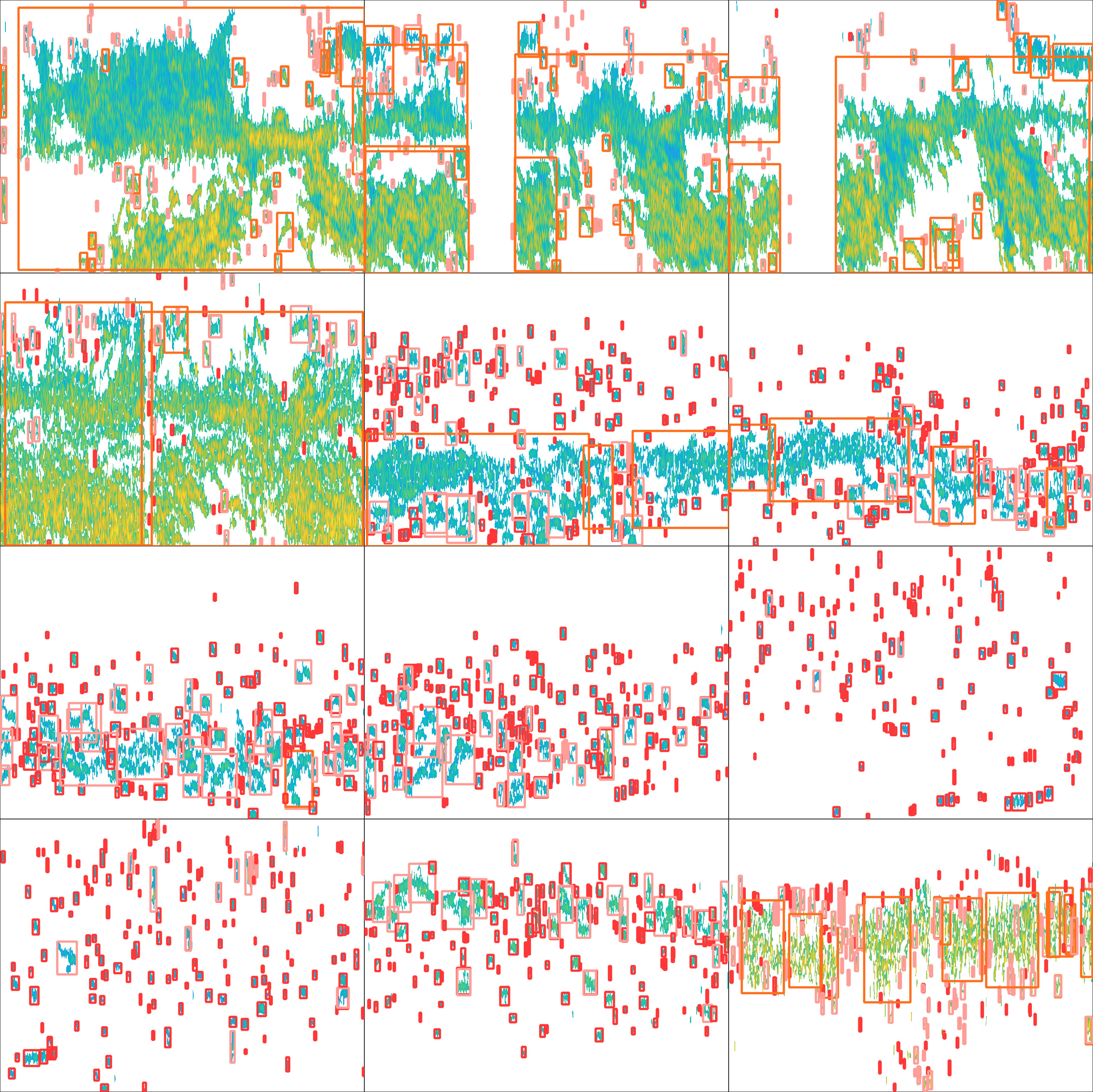
Figure 8 Automatic annotation of test set echograms.
Figure 9 shows the in situ histograms for two sampling sites with biological sampling. The maximum value of the in situ observed on June 4, 2021, was 94.35 dB, and the minimum value was 54.93 dB. The maximum value observed on July 5 was 95.58 dB, and the minimum value was 55.13 dB. The difference between the two maximum values was 1.23 dB, and the difference between the two minimum values was 0.2 dB.
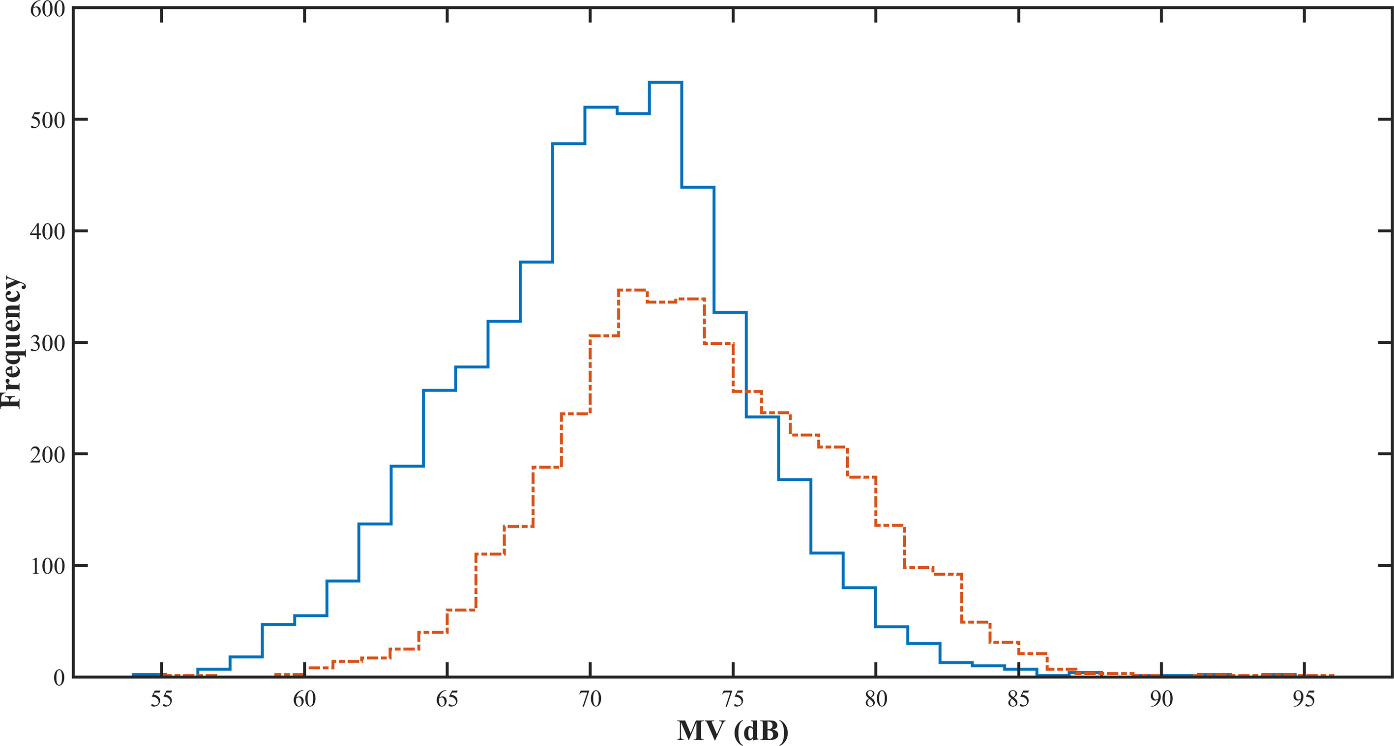
Figure 9 Observed in situ histograms of Pacific saury from two sampling sites (Jun 4, 2021, and Jul 5, 2021.) The solid blue line was sampled on Jun 4, 2021, and the dashed orange line was sampled on Jul 5, 2021.
The average, standard deviation, maximum, and minimum values of the measured body lengths of the Pacific saury samples collected at the two stations are presented in Table 3. The histogram of the calculated from the measured body lengths is shown in Figure 10. The in situ and measurements are averaged and differenced to obtain the value of living fish calibration offset . The calculated living fish calibration parameters are shown in Table 4.
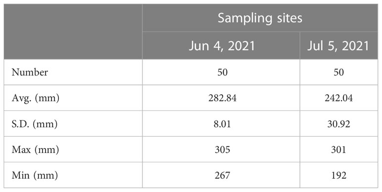
Table 3 Average, standard deviation, maximum, and minimum fork length of Pacific saury at two sampling sites, which had synchronized acoustic data and biological sampling data.
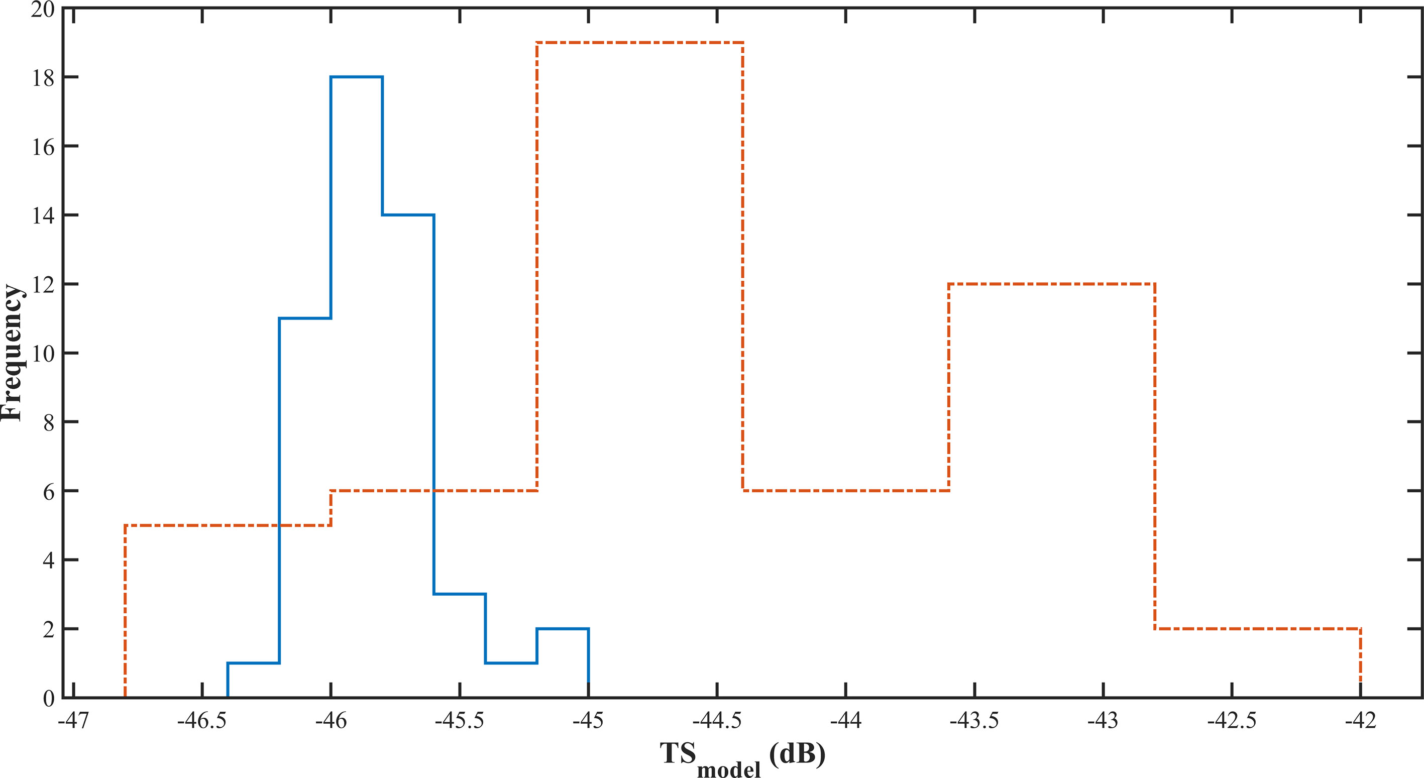
Figure 10 The of Pacific saury measured using the prolate spheroidal model. The solid blue line was sampled on Jun 4, and the dashed orange line was sampled on Jul 5.
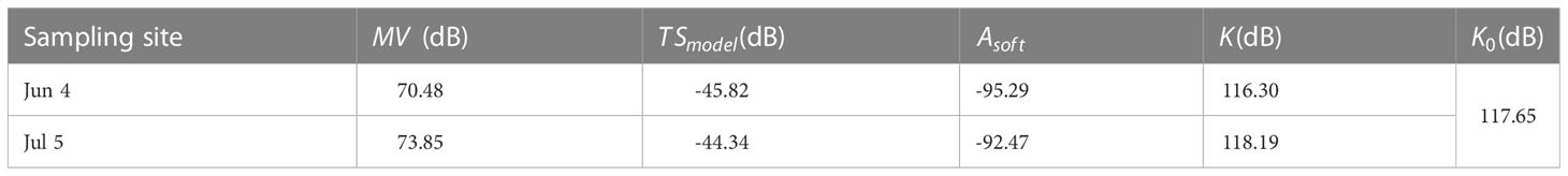
Table 4 Mean values of in situ MV, TSmodel, Asoft, and K of the Pacific saury measured at two sampling sites on Jun 4 and Jul 5; the value of K0 is measured from the standard sphere calibration process.
The data in Table 4 show that the mean in situ measured on Jun 4, 2021, was 70.48 dB and 73.85 dB on Jul 5, 2021. The mean values of the correlation coefficients for the two sites measured by the model method were -95.29 and -92.47, respectively, and the calculated values were -45.82 dB and -44.34 dB, respectively. The living fish calibration offset values were 116.30 dB and 118.19 dB, respectively. Compared with the measured from the standard sphere method calibration, the differences between and were 1.35 dB and 0.54 dB, respectively.
In this study, no training set of echo traces was available to pre-train the model. Therefore, a training set was created to train the automatic detection model for subsequent automatic detection of echo traces. The training set was created using the integral threshold setting method, median filter, and open-close operation to remove noise and reverberation from images. In the actual experiment, the noise and reverberation that were present in the original echograms (Figure 5) were removed. At the same time, the echo traces of single fish, multiple fish, and schools of fish were retained more completely (Figure 6). The method used in this study is simpler than denoising using the dB difference method (Fernandes, 2009; Brautaset et al., 2020). The reason for its simplicity is the overwhelming dominance of Pacific saury in the detected echograms and the fact that the used instrument is a single-beam with a single-frequency echo sounder.
The adopted YOLO v5 deep learning automatic detection model has a maximum value of 0.71 for mAP at intersection over union (IOU) thresholds (Redmon and Farhadi, 2018) of 0.5 and 0.43 at an IOU threshold of 0.5:0.95 after 300 rounds of training. These values indicate that the prediction accuracy is low when the set prediction box and the actual box have an overlap of 50–95%, and most targets at the set prediction box and the actual box at 50% overlap are accurately predicted. The identification accuracy of the model is higher for larger objects in the echogram and lower for smaller objects in the echogram, which is also consistent with the F1 score curve for evaluating model performance (Figure 7). The maximum F1 score of the trained automatic detection model is 0.66, which still represents a large advantage. The number of images in the training set and the resolution of the images are essential factors affecting the F1 score of the model (Chicco and Jurman, 2020; Jalal et al., 2020; Fourure et al., 2021). The single-beam echograms are sparse and contain less information in one echo trace. Therefore, more samples are needed to improve the F1 score of the trained model.
The measured in situ histogram curves were similar to those obtained by Sawada et al. (Sawada et al., 2011) when measuring the in situ target strength of Diaphus theta, in which the distribution of the value at site Jul 5, 2021, had a larger interval and a higher mean value than that at site Jun 04, 2021, and the distribution at site Jun 04, 2021, was more concentrated. The distribution of measured from the fork length at the site sampled by the PSM method was similar to the distribution of measurement values obtained in situ. The distribution of on Jun 4, 2021, was mainly concentrated between -45 dB and -46.5 dB, while the distribution on Jul 5, 2021, was in the range of -42 dB to -47 dB, which is largely different from the in situ distribution characteristics. The mean at the two sites were -45.82 dB and -44.34 dB, respectively, while the mean target strength of the Pacific saury calculated by PSM by Sawada et al. (Sawada et al., 2009) was -39.9 dB. A gap exists between the target strength calculated by the developed model and that calculated by Sawada et al. This may be caused by the following reasons: First, Sawada et al. used fewer samples for their calculations, all of which were based on “bird sampled”. This makes the target strength value selective and leads to a smaller interval distribution. Second, the frequency they used was 70 kHz, and the frequency used in the present study was 50 kHz. The target strength values of fish were different at different frequencies. In PSM calculations, the angle of inclination of the swim bladder is another important factor that affects the target strength value of fish. In this study, the typical swim bladder length to fork length ratio was substituted into the PSM model for calculations. The size of the swim bladder tilt angle was not adequately considered. Measurements of the tilt angle distribution of swim bladder are necessary in further studies.
The living fish calibration offset calculated by in situ and for the two sites differed by 1.35 dB and 0.54 dB, respectively, compared to the calibrated in the laboratory using the standard sphere method. According to the standard deviation threshold of 2 dB given by the Biosonics instrument calibration manual (Biosonics, 2004), the values obtained in the present study were within the standard range. The shipboard commercial echo sounder can carry out scientific acoustic survey work. As a rapid acoustic instrument performance testing method, the living fish calibration method is also feasible to a certain degree. The calibration method for rapid instrument performance testing can efficiently obtain more accurate acoustic survey data to expand the coverage area of fish resources. However, compared to the calibration of acoustic instruments using the standard calibration sphere method, there are still certain deviations, which mostly originate from the swimming behavior of fish and physical changes in the marine environment (Simmonds and Maclennan, 2008).
Commercial fishing vessels worldwide are commonly equipped with echo sounders for vertical detection of underwater information. However, current acoustic monitoring of fishery resources still relies on research vessels. In most cases, the underwater information detected by commercial echo sounders is not collected and analyzed. The main reasons for this situation include the absence of information such as geographic information location and time series associated with the echo intensity level; moreover, the echo sounders are often not calibrated when using fishing vessels for acoustic monitoring (Haris et al., 2021). These reasons result in the acoustic data collected by commercial fishing vessels remaining unutilized, as these data cannot be applied to classify fish species and assess resources.
The most important work of this study was the combination of the automatic detection model and the living fish calibration method to propose an echo sounder calibration method that is suitable for commercial fishing vessels. The developed method uses a deep learning target recognition method (YOLO v5) to quickly identify single fish echo traces in the echogram without the need to extract feature parameters by a manual operation before identification. Identification is based on the absolute dominance of the target fish species in the fishing process. The ease of access to target biological samples during fishing operations enables the measurement of model target strength values in a short period of time using the PSM method. The performance of the shipboard echo sounder is tested by comparing it with the in situ measurement value and deriving the offset of the acoustic data. The method can be used without impacting fishing operations. The offset is removed in a subsequent pre-processing step to make the data available for scientific research. The single-beam acoustic data used in this study are commonly available on commercial fishing vessels. The sparse nature of the single-beam data enables the acquisition of more acoustic detection areas with less storage space. The species classification results obtained by identifying single-beam data can be used for resource assessments and can aid fishing staff. For multi-species mixed fisheries, the method still needs further verification. With the development of fish detection technology, echo sounders equipped with multi-beam and broadband transducers are gradually used on fishing vessels. Of these, the broadband acoustic technique can obtain continuous echo features over the entire frequency band range, obtain a spectrogram of target echo intensity with frequency, and increase the amount of information on an individual echo trace (Xue et al., 2021). When using deep learning methods for target recognition, the developed method increases the training accuracy of the model and improves the success rate of target detection. Applying this method to broadband acoustic data is an important direction for future research.
Fishing vessels equipped with echosounders provide unique opportunities for the monitoring and assessment of fishery resources. A key challenge in the use of echo data collected from commercial echosounders is data calibration. This paper presents a deep learning method for the automatic detection of single fish echo traces. The results demonstrated that by combining the detected single fish echo traces with fishing samples, the echo data could be calibrated to a level similar to that of scientific echosounders, which aids scientific interpretation of these data. However, the current calibration method is still at a relatively moderate level, and traditional calibration with a standard sphere should be conducted whenever an opportunity arises.
The raw data supporting the conclusions of this article will be made available by the authors, without undue reservation.
ST and JT designed the study. JH and JT provided the methodology and developed the data recording equipment. WW conducted the investigation. WW, MX, and ZZ analyzed the data. WW wrote the original draft. JT reviewed and edited the draft. All authors contributed to the article and approved the submitted version.
This research was funded by the National Key R&D Program of China (2019YFD0901401) and the Key Laboratory of Marine Ecological Monitoring and Restoration Technologies (MEMRT202202). We also acknowledge funds provided by the Ministry of Agriculture and Rural Affairs of China, through the project on the Survey and Monitor-Evaluation of Global Fishery Resources.
The authors of this research would like to thank the captain and all the crews of the FV Ming Hua for providing the investigation platform and related facilities of data collection in this study. The authors also thank the China Aquatic Products Zhoushan Marine Fisheries Corporation for help with implementating the research project. The help of Taoxi Xue, a member of staff of the Yellow Sea Fisheries Research Institute, is particularly appreciated for his assistance in the survey work.
The authors declare that the research was conducted in the absence of any commercial or financial relationships that could be construed as a potential conflict of interest.
All claims expressed in this article are solely those of the authors and do not necessarily represent those of their affiliated organizations, or those of the publisher, the editors and the reviewers. Any product that may be evaluated in this article, or claim that may be made by its manufacturer, is not guaranteed or endorsed by the publisher.
The Supplementary Material for this article can be found online at: https://www.frontiersin.org/articles/10.3389/fmars.2023.1162064/full#supplementary-material
Albawi S., Bayat O., Al-Azawi S., Ucan O. N. (2018). Social touch gesture recognition using convolutional neural network. Comput. Intell. Neurosci. 2018, 6973103. doi: 10.1155/2018/6973103
Aranis A., de la Cruz R., Montenegro C., Ramírez M., Caballero L., Gómez A., et al. (2022). Meta-estimation of araucanian herring, Strangomera bentincki (Norman 1936), biological indicators in the central-south zone of Chile (32°–47° LS). Front. Mar. Sci. 9. doi: 10.3389/fmars.2022.886321
Axenrot T., Didrikas T., Danielsson C., Hansson S. (2004). Diel patterns in pelagic fish behaviour and distribution observed from a stationary, bottom-mounted, and upward-facing transducer. ICES J. Mar. Sci. 61, 1100–1104. doi: 10.1016/j.icesjms.2004.07.006
Biosonics I. (2004). Calibration of BioSonics digital scientific echosounder using T/C calibration spheres. (Seattle, WD, USA: Biosonics Inc.), 1–11. Available at: http://www.biosonicsinc.com/doc_library/docs/DTXcalibration2e.pdf.
Boswell K. M., D’Elia M., Johnston M. W., Mohan J. A., Warren J. D., Wells R. J. D., et al. (2020). Oceanographic structure and light levels drive patterns of sound scattering layers in a low-latitude oceanic system. Front. Mar. Sci. 7. doi: 10.3389/fmars.2020.00051
Boyra G., Moreno G., Orue B., Sobradillo B., Sancristobal I. (2019). In situ target strength of bigeye tuna (Thunnus obesus) associated with fish aggregating devices. ICES J. Mar. Sci. 76, 2446–2458. doi: 10.1093/icesjms/fsz131
Brautaset O., Waldeland A. U., Johnsen E., Malde K., Eikvil L., Salberg A.-B., et al. (2020). Acoustic classification in multifrequency echosounder data using deep convolutional neural networks. ICES J. Mar. Sci. 77 (4), 1391–1400. doi: 10.1093/icesjms/fsz235
Chicco D., Jurman G. (2020). The advantages of the matthews correlation coefficient (MCC) over F1 score and accuracy in binary classification evaluation. BMC Genomics 21, 6. doi: 10.1186/s12864-019-6413-7
Coetzee J. (2000). Use of a shoal analysis and patch estimation system (SHAPES) to characterise sardine schools. Aquat. Living Resour. 13, 1–10. doi: 10.1016/S0990-7440(00)00139-X
Didrikas T., Hansson S. (2004). In situ target strength of the Baltic Sea herring and sprat. ICES J. Mar. Sci. 61, 378–382. doi: 10.1016/j.icesjms.2003.08.003
Eleftherakis D., Berger L., Le Bouffant N., Pacault A., Augustin J.-M., Lurton X. (2018). Backscatter calibration of high-frequency multibeam echosounder using a reference single-beam system, on natural seafloor. Mar. Geophys. Res. 39, 55–73. doi: 10.1007/s11001-018-9348-5
Fallon N. G., Fielding S., Fernandes P. G. (2016). Classification of southern ocean krill and icefish echoes using random forests. ICES J. Mar. Sci. 73, 1998–2008. doi: 10.1093/icesjms/fsw057
Fang J., Wang P. (2021). Application of improved YOLO V3 algorithm for target detection in echo image of sonar under reverb. J. Phys.: Conf. Ser. 1748, 42048. doi: 10.1088/1742-6596/1748/4/042048
Fernandes P. G. (2009). Classification trees for species identification of fish-school echotraces. ICES J. Mar. Sci. 66, 1073–1080. doi: 10.1093/icesjms/fsp060
Fernandes P. G., Copland P., Garcia R., Nicosevici T., Scoulding B. (2016). Additional evidence for fisheries acoustics: small cameras and angling gear provide tilt angle distributions and other relevant data for mackerel surveys. ICES J. Mar. Sci. 73, 2009–2019. doi: 10.1093/icesjms/fsw091
Foote K. G., Rothschild B. J. (2009). “Acoustic methods: brief review and prospects for advancing fisheries research,” in The future of fisheries science in north america. fish & fisheries series, vol. 31 . Ed. Beamish R. J. (Dordrecht: Springer), 313–343. doi: 10.1007/978-1-4020-9210-7_18
Fourure D., Javaid M. U., Posocco N., Tihon S. (2021). “Anomaly detection: how to artificially increase your F1-score with a biased evaluation protocol,” in Machine learning and knowledge discovery in databases. applied data science track. ECML PKDD 2021. lecture notes in computer science. Eds. Dong Y., Kourtellis N., Hammer B., Lozano J. A. (Cham: Springer), 12978. doi: 10.1007/978-3-030-86514-6_1
Furusawa M. (1988). Prolate spheroidal models for predicting general trends of fish target strength. J. Acoust. Soc. Japan (E) 9, 13–24. doi: 10.1250/ast.9.13
Gjøsæter H., Wiebe P. H., Knutsen T., Ingvaldsen R. B. (2017). Evidence of diel vertical migration of mesopelagic sound-scattering organisms in the Arctic. Front. Mar. Sci. 4. doi: 10.3389/fmars.2017.00332
Gu J., Wang Z., Kuen J., Ma L., Shahroudy A., Shuai B., et al. (2018). Recent advances in convolutional neural networks. Pattern recognit. 77, 354–377. doi: 10.1016/j.patcog.2017.10.013
Haris K., Kloser R. J., Ryan T. E., Downie R. A., Keith G., Nau A. W. (2021). Sounding out life in the deep using acoustic data from ships of opportunity. Sci. Data 8, 1–23. doi: 10.6084/m9.figshare.13172516
Ito M., Matsuo I., Imaizumi T., Akamatsu T., Wang Y., Nishimori Y. (2013). “Classification of fish schools based on acoustic features associated with tilt angle,” in 2013 IEEE International Underwater Technology Symposium (UT), Tokyo, Japan. 2013, 1–4. doi: 10.1109/UT.2013.6519865
Jalal A., Salman A., Mian A., Shortis M., Shafait F. (2020). Fish detection and species classification in underwater environments using deep learning with temporal information. Ecol. Inf. 57, 101088. doi: 10.1016/j.ecoinf.2020.101088
Johannesson K., Losse G. (1977). Methodology of acoustic estimations of fish abundance in some UNDP/FAO resource survey projects. Rapports Proces-Verbaux Des. Reunions (ICES) 170, 296–318.
Julie S., Anne L. D., Paulo T., Sven G., Gildas R., Gary V., et al. (2020). In situ target strength measurement of the black triggerfish melichthys niger and the ocean triggerfish canthidermis sufflamen. Mar. Freshw. Res. 71, 1118–1127. doi: 10.1071/MF19153
Khodabandeloo B., Agersted M. D., Klevjer T., Macaulay G. J., Melle W. (2021). Estimating target strength and physical characteristics of gas-bearing mesopelagic fish from wideband in situ echoes using a viscous-elastic scattering model. J. Acoust. Soc. America 149, 673–691. doi: 10.1121/10.0003341
Knudsen H. P. (2009). Long-term evaluation of scientific-echosounder performance. ICES J. Mar. Sci. 66, 1335–1340. doi: 10.1093/icesjms/fsp025
Lawson G. L., Barange M., Fréon P. (2001). Species identification of pelagic fish schools on the south African continental shelf using acoustic descriptors and ancillary information. ICES J. Mar. Sci. 58, 275–287. doi: 10.1006/jmsc.2000.1009
Lee K. H., Lee D. J., Kim H. S., Park S. W. (2010). Swimming speed measurement of pacific saury (Cololabis saira) using acoustic Doppler current profiler. J. Korean Soc. Fish. Ocean Technol. 46 (2), 165–172. doi: 10.3796/ksft.2010.46.2.165
LeFeuvre P., Rose G., Gosine R., Hale R., Pearson W., Khan R. (2000). Acoustic species identification in the Northwest Atlantic using digital image processing. Fish. Res. 47, 137–147. doi: 10.1016/S0165-7836(00)00165-X
Li X., Shang M., Hao J., Yang Z. (2016). Accelerating fish detection and recognition by sharing CNNs with objectness learning. OCEANS 2016 - Shanghai Shanghai China 2016, 1–5. doi: 10.1109/OCEANSAP.2016.7485476
Li X., Shang M., Qin H., Chen L. (2015). Fast accurate fish detection and recognition of underwater images with fast r-cnn. OCEANS 2015 - MTS/IEEE Washington (Washington, DC: IEEE) 2015, 1–5. doi: 10.23919/OCEANS.2015.7404464
Martignac F., Daroux A., Bagliniere J. L., Ombredane D., Guillard J. (2015). The use of acoustic cameras in shallow waters: new hydroacoustic tools for monitoring migratory fish population. a review of DIDSON technology. Fish fish. 16, 486–510. doi: 10.1111/faf.12071
Melvin G. D., Kloser R., Honkalehto T. (2016). The adaptation of acoustic data from commercial fishing vessels in resource assessment and ecosystem monitoring. Fish. Res. 178, 13–25. doi: 10.1016/j.fishres.2015.09.010
O'Donncha F., Stockwell C. L., Planellas S. R., Micallef G., Palmes P., Webb C., et al. (2021). Data driven insight into fish behaviour and their use for precision aquaculture. Front. Anim. Sci. 2. doi: 10.3389/fanim.2021.695054
Rathi D., Jain S., Indu S. (2017). “Underwater fish species classification using convolutional neural network and deep learning,” in 2017 Ninth International Conference on Advances in Pattern Recognition (ICAPR). 2017, 1–6 (Bangalore, India: IEEE). doi: 10.1109/ICAPR.2017.8593044
Redmon J., Farhadi A. (2018). Yolov3: an incremental improvement. Comput. Vision Pattern Recognit. 1804, 2767. doi: 10.48550/arXiv.1804.02767
Reid D. G. (2000). Report on echo trace classification. ICES Coop. Res. Rep. 238, 1–115. doi: 10.17895/ices.pub.5371
Robotham H., Bosch P., Gutiérrez-Estrada J. C., Castillo J., Pulido-Calvo I. (2010). Acoustic identification of small pelagic fish species in Chile using support vector machines and neural networks. Fish. Res. 102, 115–122. doi: 10.3135/jmasj.20.73
Sawada K., Furusawa M., Williamson N. J. (1993). Conditions for the precise measurement of fish target strength in situ. J. Mar. Acoust. Soc. Japan 20, 73–79. doi: 10.3135/jmasj.20.73
Sawada K., Takahashi H., Abe K., Ichii T., Watanabe K., Takao Y. (2009). Target-strength, length, and tilt-angle measurements of pacific saury (Cololabis saira) and Japanese anchovy (Engraulis japonicus) using an acoustic-optical system. ICES J. Mar. Sci. 66, 1212–1218. doi: 10.1093/icesjms/fsp079
Sawada K., Uchikawa K., Matsuura T., Sugisaki H., Amakasu K., Abe K. (2011). In situ and ex situ target strength measurement of mesopelagic lanternfish, diaphus theta (Family myctophidae). J. Mar. Sci. Technol. 19, 10. doi: 10.51400/2709-6998.2196
Simmonds J., Maclennan D. N. (2008). Fisheries acoustics: theory and practice (New York: John Wiley & Sons).
Slotte A., Hansen K., Dalen J., Ona E. (2004). Acoustic mapping of pelagic fish distribution and abundance in relation to a seismic shooting area off the Norwegian west coast. Fish. Res. 67, 143–150. doi: 10.1016/j.fishres.2003.09.046
Sobradillo B., Boyra G., Martinez U., Carrera P., Peña M., Irigoien X. (2019). Target strength and swimbladder morphology of mueller’s pearlside (Maurolicus muelleri). Sci. Rep. 9, 17311. doi: 10.1038/s41598-019-53819-6
Tong J., Xue M., Zhu Z., Wang W., Tian S. (2022). Impacts of morphological characteristics on target strength of chub mackerel (Scomber japonicus) in the Northwest pacific ocean. Front. Mar. Sci. 9. doi: 10.3389/fmars.2022.856483
Trumpickas J., Pinder M., Dunlop E. S. (2020). Effects of vessel size and trawling on estimates of pelagic fish backscatter in lake Huron. Fish. Res. 224, 105430. doi: 10.1016/j.fishres.2019.105430
Tsagarakis K., Pyrounaki M., Giannoulaki M., Somarakis S., Machias A. (2012). Ontogenetic shift in the schooling behaviour of sardines, sardina pilchardus. Anim. Behav. 84, 437–443. doi: 10.1016/j.anbehav.2012.05.018
Wageeh Y., Mohamed H. E.-D., Fadl A., Anas O., Elmasry N., Nabil A., et al. (2021). YOLO fish detection with euclidean tracking in fish farms. J. Ambient Intell. Humanized Comput. 12, 5–12. doi: 10.1007/s12652-020-02847-6
Wang N., Chen T., Kong X., Chen Y., Wang R., Gong Y., et al. (2023d). Underwater attentional generative adversarial networks for image enhancement. IEEE Trans. Human-Machine Syst. 1-, 11. doi: 10.1109/THMS.2023.3261341
Wang N., Chen T., Liu S., Wang R., Karimi H. R., Lin Y. (2023a). Deep learning-based visual detection of marine organisms: a survey. Neurocomputing 532, 1–32. doi: 10.1016/j.neucom.2023.02.018
Wang H., Sun S., Bai X., Wang J., Ren P. (2023b). A reinforcement learning paradigm of configuring visual enhancement for object detection in underwater scenes. IEEE J. Oceanic Eng. 48, 2: 443–2: 461. doi: 10.1109/JOE.2022.3226202
Wang H., Sun S., Ren P. (2023c). Meta underwater camera: a smart protocol for underwater image enhancement. ISPRS J. Photogrammetry Remote Sens. 195, 462–481. doi: 10.1016/j.isprsjprs.2022.12.007
Wang H., Sun S., Wu X., Li L., Zhang H., Li M., et al. (2021). “A yolov5 baseline for underwater object detection,” in OCEANS 2021 (San Diego–Porto: IEEE), 1–4. doi: 10.23919/OCEANS44145.2021.9705896
Wang N., Wang Y., Er M. J. (2022). Review on deep learning techniques for marine object recognition: architectures and algorithms. Control Eng. Pract. 118, 104458. doi: 10.1016/j.conengprac.2020.104458
Keywords: fishing vessel, automatic detection, commercial echosounder calibration, Cololabis saira, deep learning, single fish detection
Citation: Tong J, Wang W, Xue M, Zhu Z, Han J and Tian S (2023) Automatic single fish detection with a commercial echosounder using YOLO v5 and its application for echosounder calibration. Front. Mar. Sci. 10:1162064. doi: 10.3389/fmars.2023.1162064
Received: 09 February 2023; Accepted: 22 May 2023;
Published: 05 June 2023.
Edited by:
Mark C. Benfield, Louisiana State University, United StatesReviewed by:
Philippe Blondel, University of Bath, United KingdomCopyright © 2023 Tong, Wang, Xue, Zhu, Han and Tian. This is an open-access article distributed under the terms of the Creative Commons Attribution License (CC BY). The use, distribution or reproduction in other forums is permitted, provided the original author(s) and the copyright owner(s) are credited and that the original publication in this journal is cited, in accordance with accepted academic practice. No use, distribution or reproduction is permitted which does not comply with these terms.
*Correspondence: Jianfeng Tong, amZ0b25nQHNob3UuZWR1LmNu
Disclaimer: All claims expressed in this article are solely those of the authors and do not necessarily represent those of their affiliated organizations, or those of the publisher, the editors and the reviewers. Any product that may be evaluated in this article or claim that may be made by its manufacturer is not guaranteed or endorsed by the publisher.
Research integrity at Frontiers
Learn more about the work of our research integrity team to safeguard the quality of each article we publish.