 Yumi Abe
 Shoshiro Minobe
- 1Department of Natural History Sciences, Graduate School of Science, Hokkaido University, Sapporo, Japan
- 2Department of Earth and Planetary Sciences, Faculty of Science, Hokkaido University, Sapporo, Japan
This study investigated the relationship between the observed and simulated dissolved oxygen (O2) inventory changes in the North Pacific by analyzing an observational dataset and the outputs of Coupled Model Intercomparison Project Phase 5 and 6 (CMIP5/6) between 1958 and 2005. A total of 204 ensembles from 20 models were analyzed. Many of the models in the North Pacific subarctic region have higher climatological O2 concentrations than observed at deeper water depths. Therefore, the negative trend of O2 inventories tends to be larger, and in fact, several model ensemble members have a larger negative trend in O2 inventories than observed. The variability among model ensemble members is more influenced by the uncertainty due to internal variability than by the uncertainty resulting from model dependency. An inter-model empirical orthogonal function (EOF) analysis revealed that the different simulated magnitudes of the negative O2 trend is closely associated with the first EOF mode, and ensemble members with strong negative trends are characterized by large oxygen reduction in the subarctic North Pacific, especially around the boundaries between the North Pacific Ocean and the Sea of Okhotsk as well as the Bering Seas. The modeled strong O2 decrease in the subarctic North Pacific is consistent with the spatial pattern of the observed O2 trend. Further analysis of climate models indicated that the O2 decrease in the subarctic region was primarily caused by physical factors. This conclusion is supported by the significantly high correlation is present between the potential temperature and O2 inventory trend in the subarctic region, whereas an insignificant correlation coefficient is present between dissolved organic carbon and the O2 inventory trend. However, the observations have a larger ratio of O2 inventory trend to temperature trend than any of the ensembles, and thus the relationship between O2 and temperature change in the subarctic North Pacific seen in the CMIP5/6 simulations is not exact.
1 Introduction
Ocean deoxygenation is a phenomenon in which dissolved oxygen (O2) decreases in the global oceans due to global warming (Bopp et al., 2002; Keeling and Garcia, 2002; Plattner et al., 2002; Frölicher et al., 2009). Ocean deoxygenation is caused by a decrease in the saturated oxygen concentration in the surface layer of the ocean due to warmer temperatures and weakened ventilation as well as mixing caused by enhanced stratification resulting from surface warming and freshening (Helm et al., 2011). In the past half-century, according to global observational data analysis, the global O2 inventory decreased by approximately 2% of the global O2 (Ito et al., 2017; Schmidtko et al., 2017).
No consensus is present on the accuracy of numerical experiments with respect to the observed O2 decrease. Based on the fact that discrepancies exist between observations and climate models in the Coupled Model Intercomparison Project Phase 5 and 6 (CMIP5/6), CMIP5 models indicate only 0.6% global O2 decrease compared with the 2% O2 decrease from observations over the past half-century (Oschlies et al., 2018; Grégoire et al., 2021). By contrast, Kwiatkowski et al. (2020) suggested that the global O2 concentration trend of multi-model ensemble mean of CMIP5/6 models is within the range of different observational estimates. The lack of consensus implies that further studies are needed to understand the relationships between the observed and simulated O2 changes. In particular, it should be useful to compare observations and models in an ocean basin where data availability is relatively high and strong deoxygenation has been observed. For these reasons, we focus our attention on the North Pacific.
The North Pacific has experienced strong ocean deoxygenation, contributing approximately 18% of the global O2 decrease from 1960 to 2010 (Schmidtko et al., 2017). Compared with other regions of rapid deoxygenation, such as the South Atlantic and Southern Oceans, the North Pacific has better O2 data coverage (Ito et al., 2017). This data availability suggests that the strong O2 decrease in the North Pacific detected by global analyses (Ito et al., 2017; Schmidtko et al., 2017) would be reliable and consistent with regional analyses conducted both on the western and eastern sides of the basin. The majority of O2 in the northwestern North Pacific generally decreased in the subsurface (200–600 m) (Ono et al., 2001; Takatani et al., 2012; Sasano et al., 2015). In the eastern North Pacific, O2 concentrations increased from the 1950s until the 1980s, after which they continued to decrease, with particularly large declines near the surface (Whitney et al., 2007; Mecking et al., 2008; Crawford and Peña, 2016; Ross et al., 2020). Observed O2 changes in the North Pacific are correlated with cycles of natural variability, such as the Pacific Decadal Oscillation, North Pacific Gyre Oscillation, and 18.6-year period tidal mixing (Andreev and Baturina, 2006; Stramma et al., 2020). Moreover, O2 decreases in the northwestern North Pacific are suggested to be attributed to a decrease in sea ice (Nakanowatari et al., 2007; Sasano et al., 2018).
The spatial pattern of the O2 trend in the CMIP5 multi-model mean is uniform compared with that of observations, and it does not reproduce the distribution and amplitude of the observed O2 trend (Stramma et al., 2012; Oschlies et al., 2017); although, for both global and North Pacific O2 concentrations, a high correlation exists between CMIP5/6 model outputs and observed climatology in subsurface waters (Takano et al., 2018; Figure 4 in Séférian et al., 2020). It should be noted, however, that the CMIP model tends to overestimate climatology in the North Pacific interior (Takano et al., 2018). A hindcast model experiment to simulate the effects of physical and biological factors on O2 changes in the North Pacific showed that O2 variability is dominated by ventilation and circulation, and that the effects of biological factors are limited to 30°N–40°N (Deutsch et al., 2006). Furthermore, a hindcast experiment conducted with the Community Earth System Model experiment showed that O2 changes in the North Pacific are caused by Pacific Decadal Oscillation-linked changes in seawater temperatures that alter the depth of the isopycnal surface (Ito et al., 2019). However, it has not been investigated whether climate models capture the observed North Pacific O2 changes within the range of uncertainties of model ensemble members.
This study aims to determine whether the past O2 changes in the North Pacific are consistent or not between observations and CMIP model ensemble members. To this end, we compare the observations with 204 ensembles of 20 CMIP5/6 models. Using nearly 200 ensemble members, including six models with more than 10 ensemble members, allows us to assess how well climate models capture the observed changes including internal variability, which has a significant effect on O2 changes in the North Pacific. Whether or not the observations are included in the ensemble members’ variability is important in assessing the validity of the models.
The uncertainty in climate simulations is generally considered to arise from scenario uncertainty, model dependency, and internal variability (Hawkins and Sutton 2009) and the partitioning of these uncertainties should be studied for future ocean deoxygenation (Frölicher et al., 2016). Because we use only historical simulations, there is no scenario uncertainty, and thus only the internal variability and model dependency are the sources of uncertainty. To separate these two sources of uncertainty, large ensembles of Earth system models are useful (Maher et al., 2021). The use of a large ensemble in climate simulations allows for the internal variability to be identified as differences among ensemble members, as the initial conditions in climate simulations need only be perturbed slightly to rapidly randomize climate changes over specific time slices. Differences in response to external forcings, that is, model dependency, can be identified by using the ensemble mean as a common response among ensemble members (Deser et al., 2014).
The remainder of this paper is organized as follows. In Section 2, we describe the observational dataset and the CMIP model ensemble members used in this study. In Section 3, we first compare the O2 inventory changes in the North Pacific of the observations and those of the model ensemble members. Subsequently, the characteristics of a common spatial pattern among the model ensemble members are described. In Section 3, environmental factors related to the dominant spatial pattern among the model ensemble members are described. A discussion, including a summary of this study, is presented in Section 4.
2 Data and methods
Gridded O2 concentration anomaly data produced by Ito et al. (2017) are used in this study on a 1° × 1° scale, with data from the surface to a depth of 1000 m, comprising 47 layers from 1950 to 2015 in annual intervals. The gridded anomaly data is generated using simple objective mapping with a Gaussian weight function, whose length scales are 1000 km and 500 km in the zonal and meridional directions, respectively. If there are insufficient observations for a grid, the grid value is considered as a missing value. Reflecting the changes in the observation numbers in Boyer et al. (2013), the temporal data coverage was relatively poor during the 1950s and 2010s. Thus, our analysis period is selected from 1958 to 2005, and our analysis domain is the North Pacific (15°N–65°N, 140°E–100°W).
We analyze the outputs of 10 CMIP5 and CMIP6 models each, that is, 20 models in total, for their historical simulations (Table 1). The model outputs on the original grid shown in Table 1 are re-gridded to a common 1° × 1° grid both in latitude and longitude using bilinear interpolation, and the vertical layers are interpolated to match the 47 layers of WOD13 from the surface to 1000 m. To determine whether artificial trends of substantial magnitudes occurred in historical simulations, the O2 inventory trends in the piControl experiment were examined. We compare the O2 inventory trends calculated by subtracting the trend of O2 concentrations for the entire period of the piControl experiment from O2 concentration of the historical simulation for all model ensembles with the O2 inventory trend calculated without subtracting the trend from the piControl experiment. There is little difference between the O2 inventory trends calculated using these two methods. Thus, in this study, trend subtraction from the piControl experiment is not conducted. We analyze ensembles available for each model (Table 1) to assess the impact of internal variability on the O2 changes. The total ensemble number is 204, which is approximately one order of magnitude greater than the number of ensemble members used in previous studies of CMIP5/6 analyses (23 models in Kwiatkowski et al., 2020).
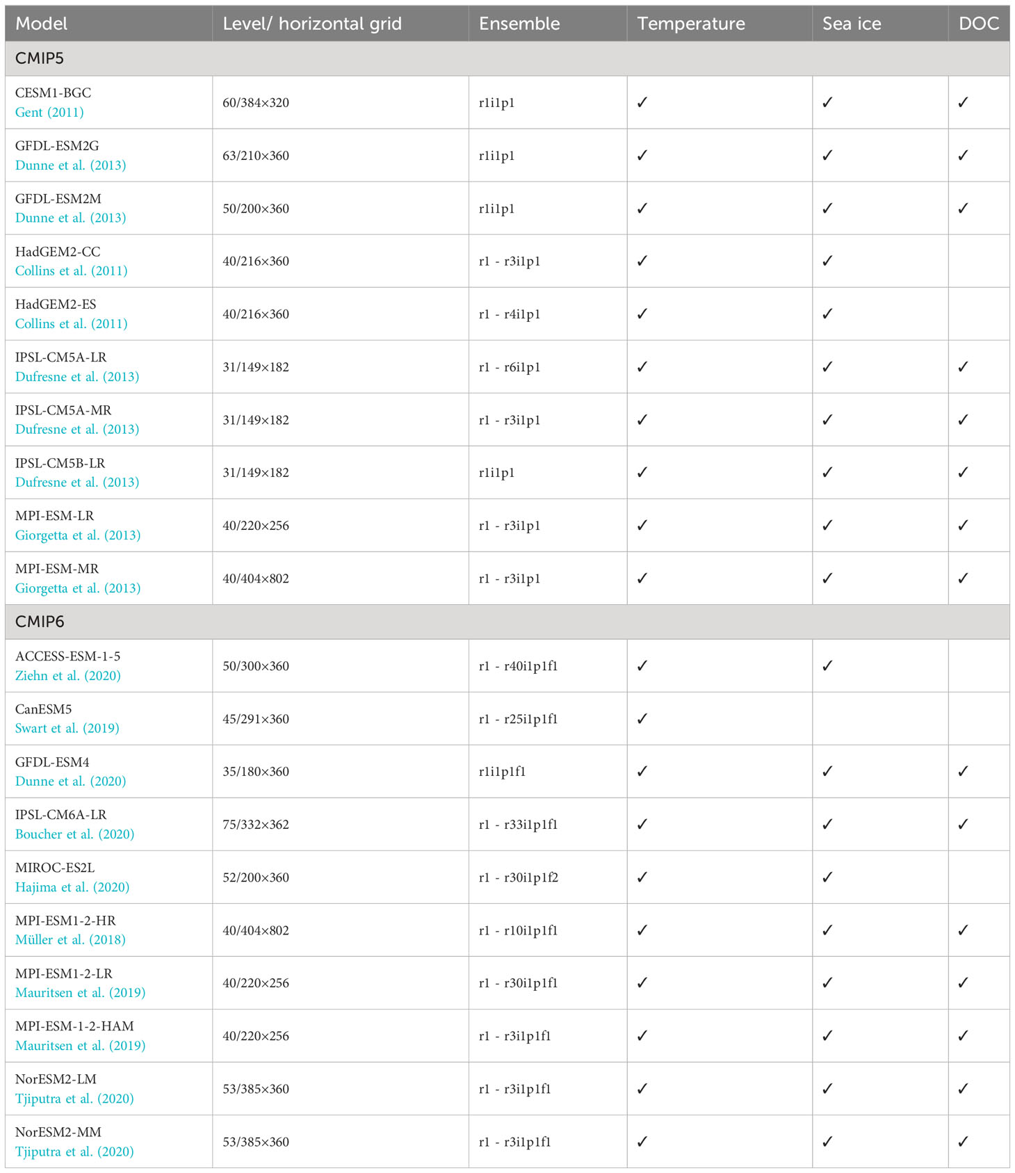
Table 1 Coupled Model Intercomparison Project (CMIP) models used in this study.
To determine the extent of the influences of physical and biological factors on O2 changes in the CMIP model, we examine the potential temperature, sea ice volume, and dissolved organic carbon (DOC). The change in potential temperature due to global warming and internal variability is the primary driver of important physical changes for O2 changes, including solubility, stratification, circulation-driven changes, and vertical migration of isopycnal surfaces. Another physical variable in this study is the sea ice volume, which is related to the formation of dense shelf water in the Okhotsk Sea which supplies O2-rich water to the northwestern North Pacific. On the other hand, DOC is related to biological factors, such as remineralization by microbial respiration, and the relationships between DOC and O2 utilization in the interior ocean have been widely studied (Doval and Hansell, 2000; Carlson et al., 2010). Also, DOC is the variable with the most model outputs for variables related to three-dimensional organic carbon in the model ensembles used in this study. The outputs of each variable are listed in Table 1.
For sea ice volume calculations, we use the same method as in Notz and SIMIP Community (2020). For the CMIP6 models, when a variable of sea ice volume is provided, sivoln, the short variable name in ESGF, is directly used; if it was not provided, we multiply a variable of sea ice volume per grid cell area, sivol, by the individual grid point area. If neither sea ice volume nor value per grid cell area is provided, we multiply the variables of sea ice concentration, siconc, sea ice thickness, sithick, and individual grid point area. For the CMIP5 models, only the variables of sea ice concentration and sea ice thickness are provided; thus, we multiply these variables and individual grid point areas. The trends in sea ice volume are calculated using the maximum sea ice volume between November and March each year.
In addition to the gridded observational O2 data and CMIP5/6 data, we use temperature and salinity data to compare the simulated temperature changes with observations and calculate saturated oxygen concentrations. The data are obtained from the World Ocean Atlas 2018 (WOA18) (Garcia et al., 2019; Locarnini et al., 2019; Zweng et al., 2019), Met Hadley Centre’s EN4.2 gridded data (Good et al., 2013), and Japan Meteorological Agency’s (JMA) gridded data ver. 7.3.1 (Ishii et al., 2017). The outputs of all variables are re-gridded to a common 1° × 1° grid and interpolated to standard ocean depth. Because the WOA18 data are provided only for decadal climatologies on an average per 10 years from 1955 to 2004, the trend is calculated for this period. We use all available gridded data of temperature and salinity.
To estimate the observed O2 inventory in the North Pacific, we use a same calculation method by Ito et al. (2017), using the following equation:
where is the inventory of O2, is the anomaly of O2 concentration, is the position vector, is the year, is the total volume of the ocean, and is the integrated volume of grid cells where the O2 data exists. Because grid cells where O2 data are available differ annually, the correction factor is applied. The volume integration is based on the same standard depths of WOD13.
In this study, six models (ACCESS-ESM1-5, CanESM5, IPSL-CM6A-LR, MIROC-ES2L, MPI-ESM1-2-HR, and MPI-ESM1-2-LR) with more than 10 ensemble members are considered as models with a large ensemble. The uncertainty of model dependency in the O2 inventory trend is expressed as the standard deviation among the ensemble means of each model. Furthermore, the uncertainty associated with internal variability is calculated by averaging the values of the standard deviations among the O2 inventory trends for ensemble members of each model. We use an empirical orthogonal function (EOF) analysis on the spatially distributed linear trend of O2 concentration at each horizontal grid point averaged from the surface to a depth of 1000 m across the 204 model ensemble members (known as the inter-model EOF analysis (Zheng et al., 2016; Zhang et al., 2023)) to determine representative O2 trend patterns among ensemble members. We use this analysis because we hypothesize that the representative pattern differences across model ensemble members could be related to the varying magnitudes of O2 inventory trends and influencing mechanisms of the trends. The inter-model EOF is calculated as follows: First, for each model ensemble member, the linear trend of O2 concentration is calculated at each horizontal grid point, averaged from the surface to depths of 1000 m as , where is the latitude, is the longitude, and is the number assigned to the model ensemble members (i.e., 1 to 204). The multi-model ensemble mean (MMEM), , across 204 ensemble members of the trend is subtracted from trends of respective ensemble members, yielding deviations in trends of respective ensemble members as, . The inter-model EOF analysis expands the O2 trend deviation as follows:
where is the spatial pattern of the nth mode, and is the model loading, which represents the amplitude of the spatial pattern for each model ensemble member.
3 Results
3.1 Oxygen inventory changes
First, we conduct a comparison to assess the consistency between the O2 climatology in the models and observation. As shown later, the subarctic region between 40°N and 65°N is the dominant region in the models for the overall O2 change in the North Pacific. Therefore, we present Figure 1 which shows the vertical distribution of regionally averaged climatological O2 concentration in the subarctic region. At depths greater than 200 m, most models have higher climatology than observation, and the difference with observation increases as the depth increases until around 700 m depth, where the decrease in observed O2 climatology levels off. This inconsistency between the climatologies of models and observations should be taken into account when comparing the modeled O2 inventory trend with observations, because models may not well reproduce water mass or O2 consumption by organisms.
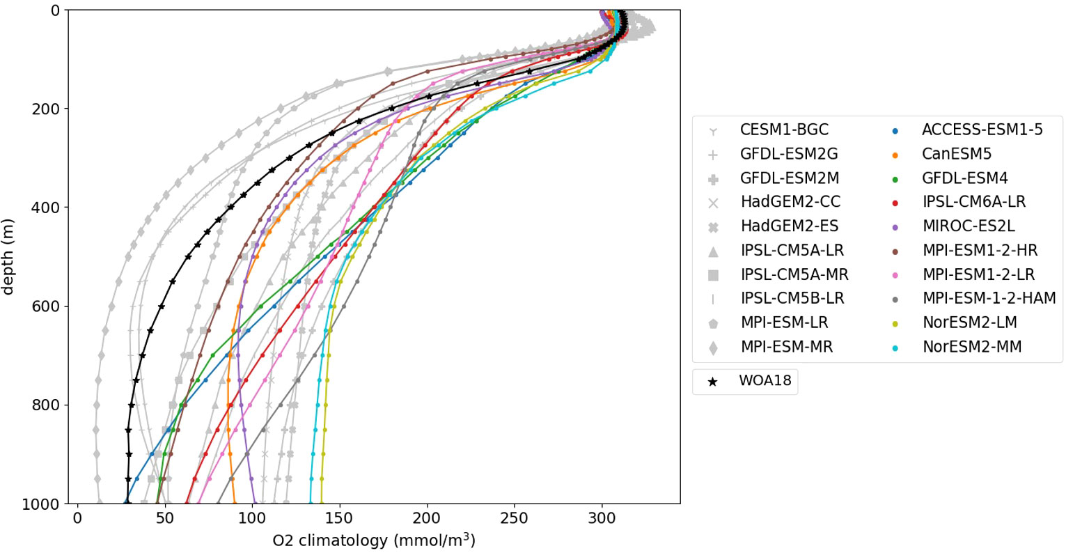
Figure 1 Vertical profile of regionally averaged O2 climatology in the subarctic region (40° to 65°N). Gray symbols represent the CMIP5 models and colored symbols represent the CMIP6 models. The black line shows the climatology based on the Garcia et al. (2019).
The observed and simulated time series of O2 anomaly inventories in the North Pacific are shown in Figure 2. The observed O2 inventory generally increased until approximately 1990, followed by large negative anomalies in the late 1990s and the early 2000s. An increase in the O2 inventory in the early period is also found in previous global observational analyses (Garcia et al., 2005; Ito et al., 2017). The record-low O2 concentrations occurred in the Oyashio area during the late 1990s (Sasano et al., 2018), which are also observed at Station P in the early 2000s (Whitney et al., 2007). The simulated O2 inventories show large diversity in their temporal evolution. The multi-ensemble mean increases until the mid-1980s and later decreased; however, each ensemble member exhibits substantial differences. Some ensemble members generally increase, whereas others generally decrease, and some increase in earlier decades and subsequently decreased. Regardless of the diversity of simulated O2 inventories, no ensemble member shows large negative anomalies in the late 1990s and the early 2000s, as observed.
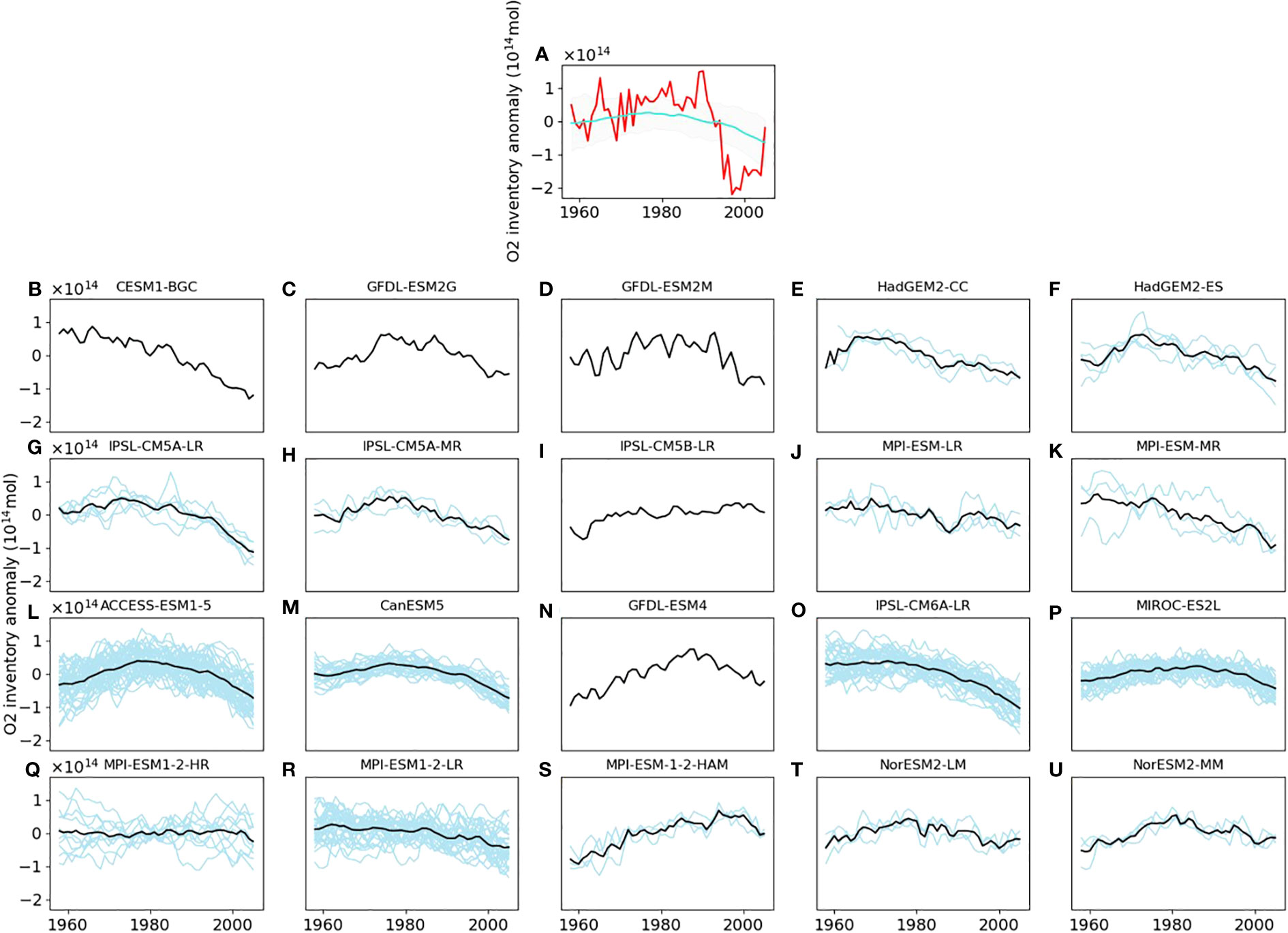
Figure 2 Anomalies in the O2 inventory from the surface to depths of 1000 m in the North Pacific from 1958 to 2005. In panel (A), the red and cyan lines indicate observed and MMEM inventories, respectively, whereas the shaded area indicates the range between the 95 and 5 percentiles among model ensemble members for each year. In panel (B–U), the light blue lines represent the ensemble members, respectively and the black line is the ensemble mean.
To evaluate how representative model skill in the North Pacific is for the global ocean, we examine the relationship between the regional and global difference in the observed and model O2 inventory trend. The relationship is obtained by (i) computing the O2 inventory trend difference for each ensemble member, and (ii) computing the correlation coefficient for the relationship between inventory trend difference in the North Pacific and the global ocean. We find a correlation coefficient of 0.535, which is statistically significant. However, it must be noted that the share of total O2 observations in the north Pacific is about 10% greater than the North Pacific’s share of the global ocean area.
Figure 3 shows the spatial patterns of the trends of the vertically averaged O2 concentrations in the observations and MMEM values. The observed trend is characterized by a strong decrease in the subarctic North Pacific, including the northwest North Pacific, especially around the Kuril Islands, between the Sea of Okhotsk and the North Pacific; around the Bering Sea; in the Gulf of Alaska; and offshore California, consistent with previous regional observational studies for the northwest North Pacific (Nakanowatari et al., 2007) and offshore California (Pierce et al., 2012; Crawford and Peña, 2016). However, the spatial pattern of the MMEM trend displays more uniformity than the observed trend.
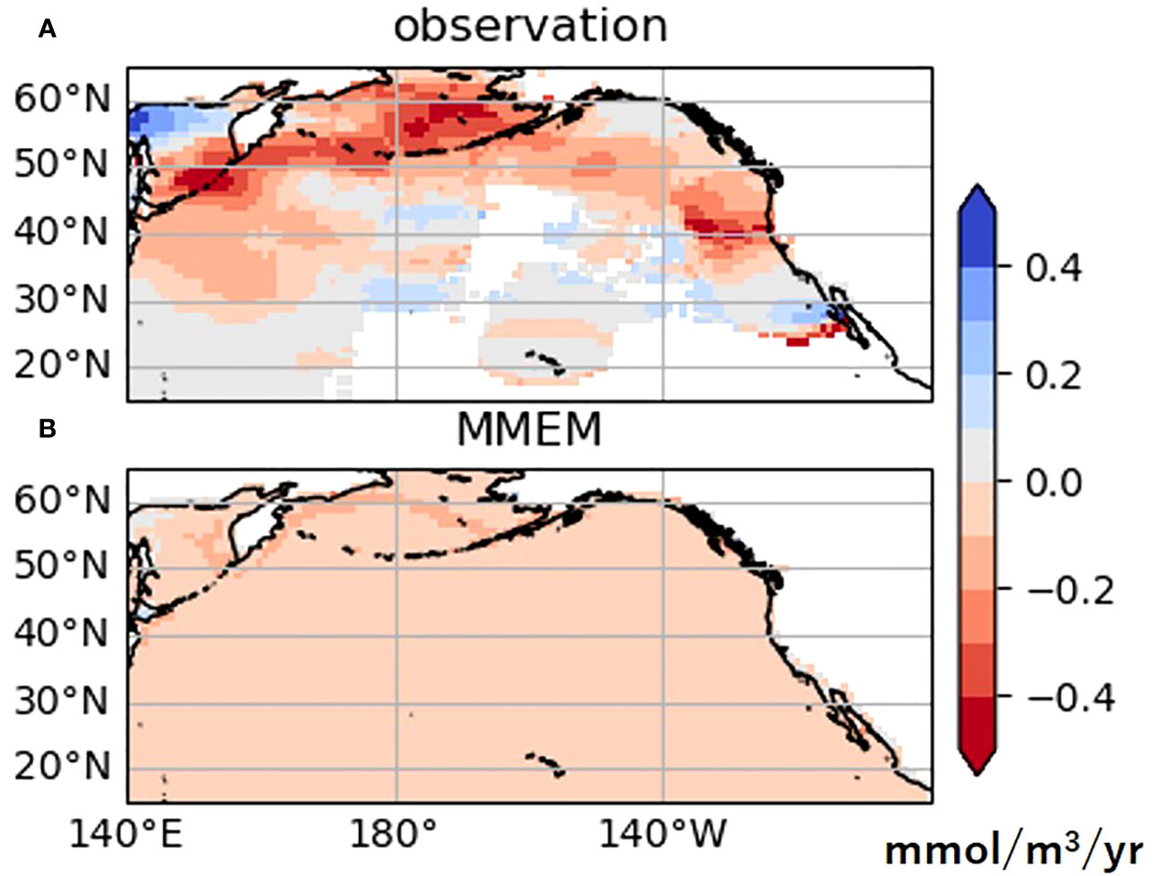
Figure 3 Vertical averages of O2 concentration trend from 1958 to 2005 in (A) observations, and (B) MMEM.
Figure 4 shows the linear trends of the O2 inventory anomaly from 1958 to 2005 in the observation and models. The observed trend of -3.52×10¹² mol/yr is thrice as large as the MMEM trend (-1.02×10¹² mol/yr). Although the observed trend is higher than the simulated trend, it is included in the variability of the simulation. 19 model ensemble members out of 204 ensemble members (i.e., 9.3%) have larger than observed negative O2 trends. Figure 4 also suggested that internal variability plays an important role in the uncertainty of the modeled O2 trend, as displayed by the positive and negative trends for different ensembles (HadGEM2-ES, IPSL-CM5A-MR, MPI-ESM-LR, MPI-ESM1-2-HR, ACCESS-ESM1-5, CanESM5, IPSL-CM6A-LR, MIROC-ES2L, MPI-ESM1-2-HR, MPI-ESM1-2-LR, and NorESM2-MM). To assess the impact of internal variability on the variability of O2 inventory trends across model ensemble members, we calculate the uncertainty of model dependency and internal variability. We obtain the uncertainty of model dependency is 8.73×10¹¹ mol/yr and internal variability is 1.65×10¹² mol/yr, respectively. The uncertainty in the O2 inventory trend due to internal variability is larger than the uncertainty due to model dependency, affecting the differences in O2 inventory trends among the models. It can be concluded that the models adequately capture the O2 trend observed. However, as previously mentioned, it is important to consider that many models have higher climatological values than observations. In particular, IPSL-CM6A-LR and MPI-ESM1-2-LR include the observed trends within the ensemble member variability, but the large difference in climatology between these models and observations from Figure 1 suggests that the models do not correctly reproduce the physical field or effect of organisms, and that O2 may not be decreasing for the same reasons as observed.
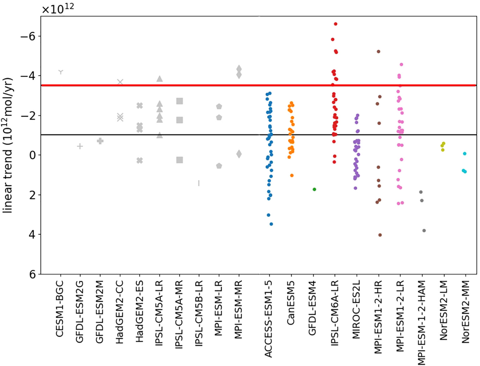
Figure 4 Trends of O2 inventory anomalies from 1958 to 2005 in the North Pacific from the surface to depths of 1000 m, with negative trends represented by upward bars. The red line shows the observational trend, and the black line shows the MMEM trend. Gray symbols represent the CMIP5 models and colored symbols represent the CMIP6 models.
3.2 Relationship between the oxygen inventory and spatial patterns
In contrast to the spatially uniform MMEM trend (Figure 3B), the model ensemble members generally show pronounced spatial structures of the O2 concentration trends. Figure 5 shows the standard deviation of the O2 concentration trend averaged from the surface to 1000 m. The variability of the trend is particularly large in the western subarctic, the Bering Sea, and especially the Sea of Okhotsk. The locations with the greatest variation among these model ensemble members are, as noted above, those with the largest negative trends in the spatial pattern of trends in the observations shown in Figure 3A.
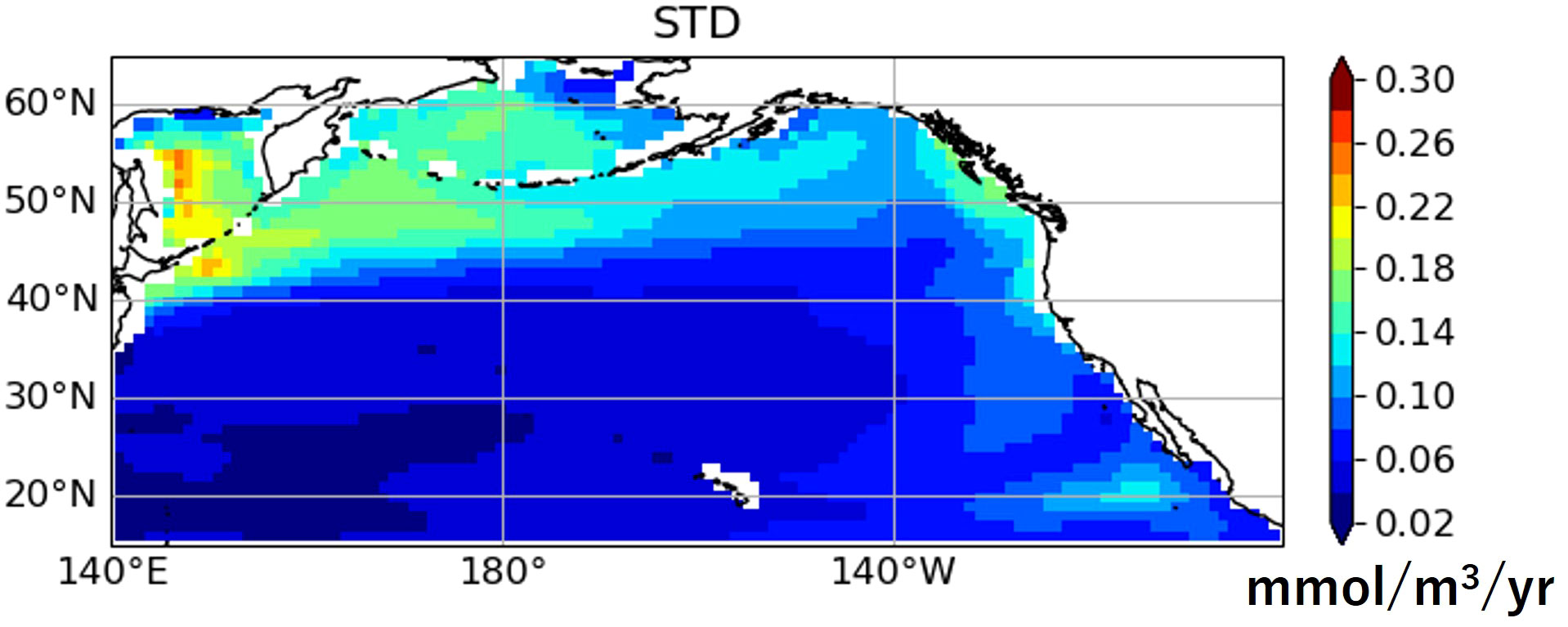
Figure 5 Standard deviation of the vertical averages of O2 concentration trend in 1958–2005 of the all model ensemble members.
To investigate whether there is a relationship between the inter-model variability in the spatial pattern of O2 trends and inter-model variability in regionally-integrated O2 inventory trends, we examine the spatial patterns of vertically averaged O2 trends for model ensemble members with large negative O2 inventory trends and those with large positive O2 inventory trends. We specifically compare the ensemble member with the largest negative trends and the ensemble member with the largest increase trends within the top four models (ACCESS-ESM1-5, IPSL-CM6A-LR, MPI-ESM1-2-HR, and MPI-ESM1-2-LR) characterized by the highest variability in O2 inventory trends within each model shown in Figure 4. From Figure 6, it is evident that ensemble members with large negative O2 inventory trends show strong negative trends in the subarctic region, the Sea of Okhotsk, and the Bering Sea. On the other hand, ensemble members with large positive O2 inventory trends show a corresponding distribution of positive trends in those regions. In IPSL-CM6A-LR, the negative trend in the Sea of Okhotsk is large in the ensemble member showing a positive trend in O2 inventory. Looking at each depth level in detail, although the negative trend is large in all depth level in the Sea of Okhotsk, the positive trend is largely distributed in the subarctic region at depths of 300 m and deeper. While the vertically averaged trend diminishes the pronounced positive trend, it is likely that this ensemble member demonstrates a positive trend in the O2 inventory trend due to the substantial positive trend in the subarctic region at deeper depths as in other models. Therefore, it is suggested that the differences in trends in the subarctic region, the Sea of Okhotsk, and the Bering Sea also affect the differences in O2 inventory trends.
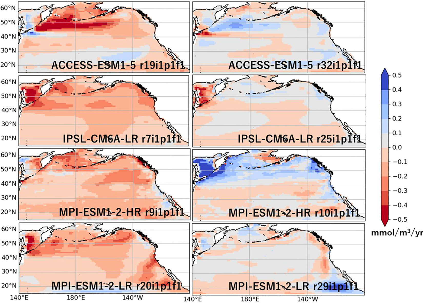
Figure 6 Vertical averages of O2 concentration trends from 1958 to 2005 in the top four models known for their large variability in O2 inventory trend (as shown in Figure 4). The left panels are the ensemble members characterized by the largest negative O2 inventory trend, while the right panels exhibit the ensemble member with the largest positive O2 inventory trend.
To extract the representative spatial patterns of the vertically averaged O2 concentration trend, inter-model EOF analysis is applied as explained in Section 2. The explained variance of the first mode was 0.28, which is much higher than that of the second mode (0.10). Figures 7A, B show the model loadings and spatial pattern, respectively, for the first EOF mode. As the spatial pattern indicates strong negative amplitudes in the subarctic North Pacific, especially in the western part and Sea of Okhotsk, ensemble members with positive loadings imply that their negative O2 trend in this region is larger than that of the MMEM. Therefore, it is expected that a higher loading would result in a more pronounced negative trend, indicating a potential correlation between the loadings and the O2 inventory trend.
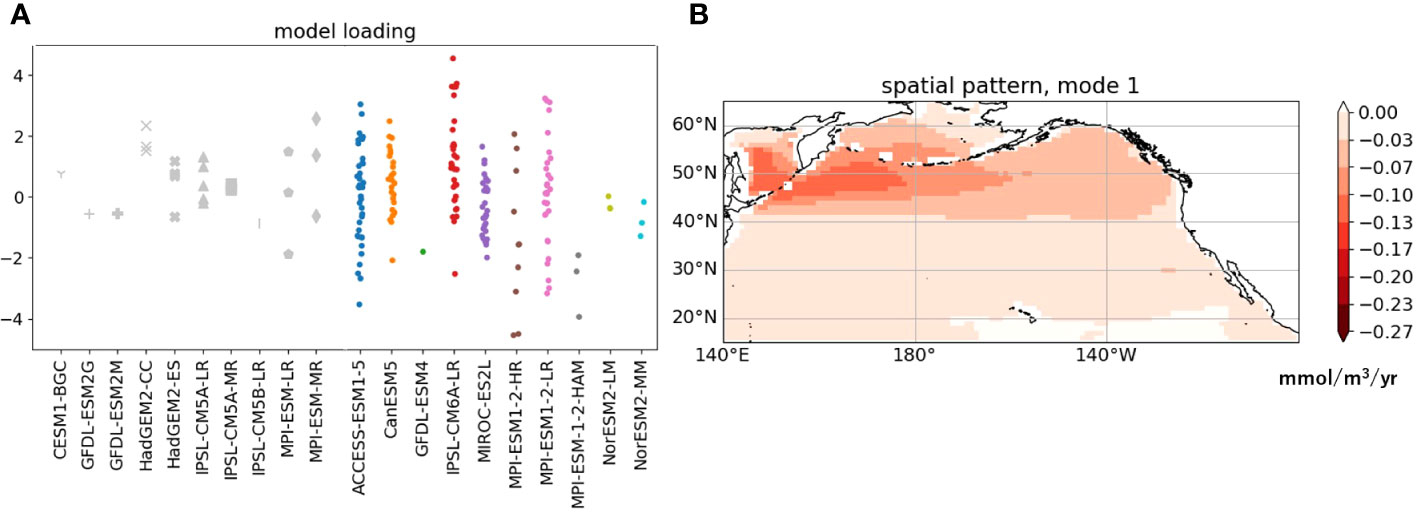
Figure 7 (A) Loading of the first Empirical orthogonal function (EOF) mode of the vertical averaged O2 concentration trend from 1958 to 2005 in model ensemble members, (B) spatial distribution of the first mode, and the color bar in (B) shows a different range from the color bars in Figures 3, 6. In (A), symbols are the same as Figure 4.
Figure 8A shows a scatter plot of the loadings of the first EOF mode shown in Figure 7A and the O2 inventory trends in Figure 4. The correlation coefficient between them is significant at -0.88 (p<0.01); thus, this relationship accounts for approximately two-thirds of the variance of the O2 inventory trends among ensemble members. Therefore, ensemble members with the largest, positive loadings on the first EOF mode have a stronger negative trend in O2 inventories. Since the largest negative amplitudes of the first EOF occur in the subarctic north Pacific, the strong negative relationship between the loadings and the simulated trend in the O2 inventories suggests that these simulated trends are mainly driven by inter-model variability in the subarctic north Pacific.
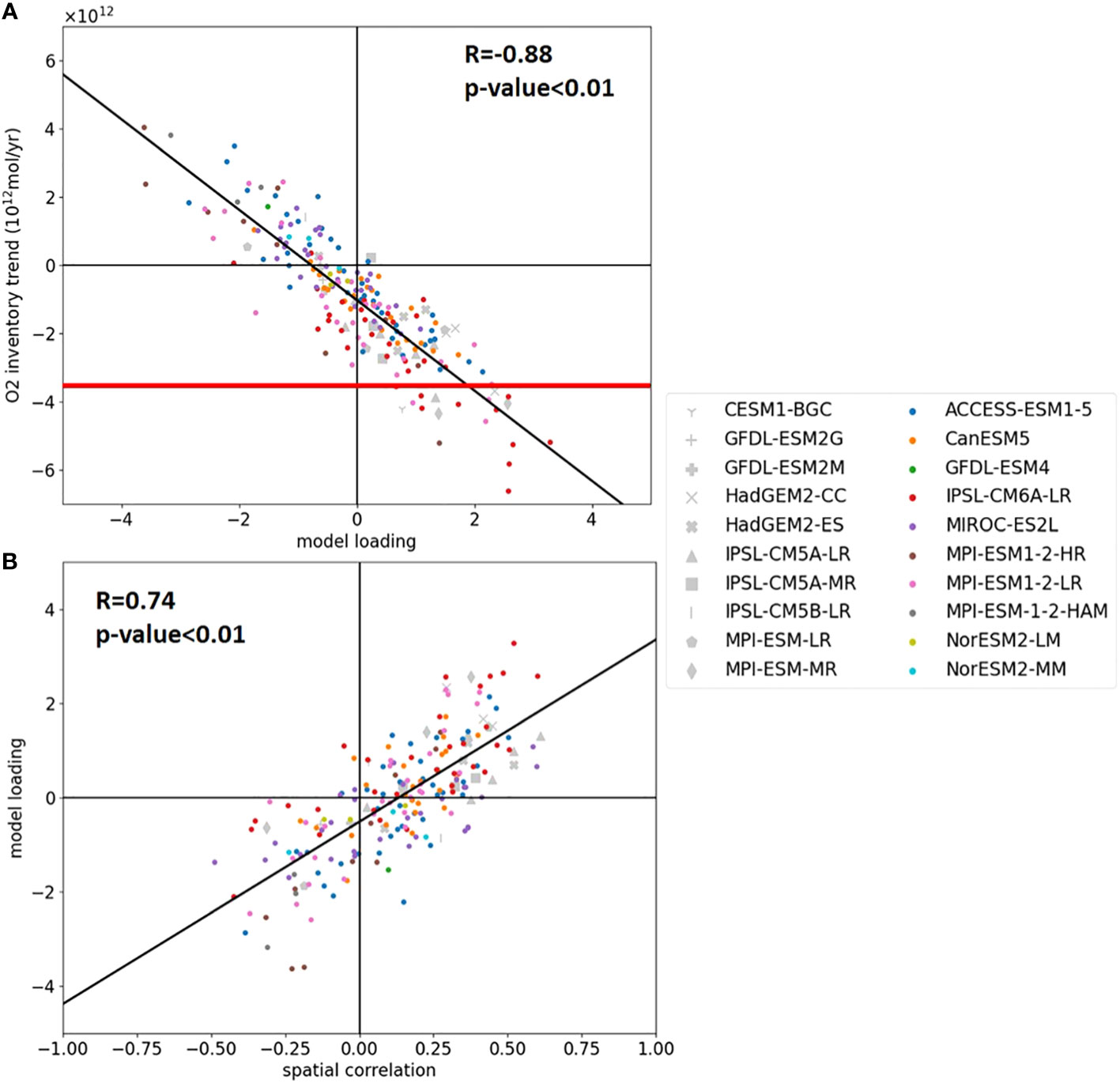
Figure 8 Scatter plots of the model loadings of the first EOF mode of the spatially distributed O2 trend and (A) the O2 inventory trend and (B) spatial correlation between the observation and each model ensemble member. The red line shows the observational trend. Gray symbols represent the CMIP5 models and colored symbols represent the CMIP6 models. Symbols are the same as Figures 4, 7A.
To ascertain whether the factors that result in the spatial pattern of the first EOF mode are consistent with the factors that reduce dissolved oxygen in the observation, it is important to investigate whether model ensemble members with positively high loading have a spatial pattern similar to the observations. Therefore, we analyze the relationship between the EOF loadings and the similarity in the spatial pattern of the O2 trend in the North Pacific between the ensemble members and observation, using spatial correlation coefficients in vertically averaged O2 concentration trends between the observation and each ensemble member as a measure of similarity (Figure 8B). The correlation coefficient between the EOF loadings and the spatial correlation coefficients is 0.74 (p<0.01); therefore, the spatial patterns of the model ensemble members with high loadings are similar to those observed in association with strong O2 reduction in the subarctic North Pacific. An ensemble member that has a strong negative trend in this region, indicating a closer resemblance to the observed trend pattern, tends to exhibit a stronger decrease in O2 throughout the basin.
3.3 Environmental factors of oxygen decrease
The results of the previous subsections indicate the importance of O2 changes in the subarctic North Pacific in observations and simulations. To determine why O2 trend variability between models is greater in the North Pacific subarctic, and whether it is consistent with observed O2 trend variability, this section discusses environmental factors that can influence O2 variation in that region. We first examine the oxygen saturation (O2sat) and apparent oxygen utilization (AOU). Here, O2sat is calculated according to the equation by Garcia and Gordon (1992), using temperature and salinity data. Temperature and salinity data are obtained from EN4, JMA, and WOA18. The AOU is calculated as AOU=O2sat-O2, where the O2 value from observations is estimated by adding the climatological O2 concentration from WOA18 to the O2 anomaly from Ito et al. (2017). We used the WOA18 annually averaged climatology from 1960 to 2017. To determine the extent to which the O2 inventory trend is explained by the AOU inventory trend and the O2sat inventory trend, we calculate the ratio of the AOU and O2sat inventory trends to the O2 inventory trend, respectively. The AOU inventory trends dominate the observed O2 and simulated inventory trends in the subarctic North Pacific. The AOU inventory trend accounts for approximately 100% of the observed O2 inventory trend. To examine the contributions of O2sat and AOU to ensemble member differences, we use multiple regression analysis to obtain partial regression coefficients for O2sat and AOU inventory trends related to O2 inventory trend in the subarctic North Pacific. The partial regression coefficient of the O2sat inventory trend on the O2 inventory trend is 0.0096, and that of the AOU inventory trend against the O2 inventory trend is -0.98. Thus, the O2 inventory trend in the subarctic North Pacific is dominated by the AOU inventory trend in the model ensemble members.
Next, we examine the influence of the physical and biological environmental factors, that is, ocean temperature, sea ice, and DOC, on the O2 inventory trends in the subarctic North Pacific. Subarctic inventory trends are calculated for temperature and DOC at each grid point and averaged in the subarctic North Pacific from the surface to depths of 1000 m, between 40°N and 65°N. For sea ice, the inventory trend of the sea ice volume is calculated by horizontal integration of sea ice volume at each grid point.
The correlations between these variables and subarctic O2 inventory trends are used to determine their relationship with the O2 change in the subarctic North Pacific. Figure 9 shows the relationship between the subarctic O2 inventory and the trend for each environmental factor. The potential temperature had a correlation of -0.24 (p<0.01), and the sea ice volume had a moderate correlation of 0.19 (p=0.011). The correlation coefficient between the temperature trends and sea-ice trends is -0.62 (p<0.01). The correlation coefficient with DOC is small and insignificant, even at the 10% significance level. The observed O2 inventory trend in the subarctic North Pacific is higher than that in most of the ensembles, while 68.5% of the total 204 ensemble members show a stronger positive temperature trend than observed. This suggests that the model underestimates the decrease in O2 in response to increasing water temperature.
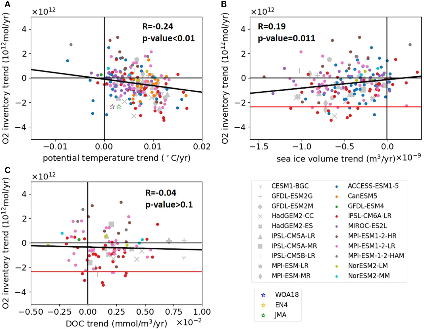
Figure 9 Scatter plots of the O2 inventory trend in the subarctic North Pacific and (A) potential temperature trend, (B) sea ice volume trend, and (C) DOC trend averaged in the subarctic North Pacific (40° to 65°N). Symbols are the same as Figure 8. Star symbols in (A) show the trends of the observations. The red line in (B, C) shows the observational trend.
Figure 9A shows that the correlation between potential temperature and O2 inventory trend is not strong. However, the regression map between the O2 inventory and the potential temperature trend in the North Pacific shown in Figure 10 indicates that potential temperature changes in the western subarctic region and the Sea of Okhotsk have a strong influence on the O2 inventory trend. In fact, the correlation coefficient between potential temperature around the Sea of Okhotsk (45° to 65°N, 140° to 160°E) and the North Pacific O2 inventory trend was highly correlated at -0.55. For SST, the relationship with the North Pacific O2 inventory trend has the same spatial pattern as in Figure 10. This spatial pattern is not entirely consistent with the PDO spatial pattern consisting of the SST anomaly which is one sign in the central and western North Pacific and the opposite sign along the eastern North Pacific (Mantua et al., 1997).
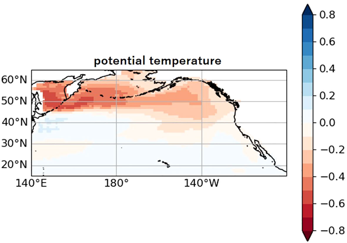
Figure 10 Correlation map between O2 inventory trend in the North Pacific and vertical averaged potential temperature among the model ensemble members.
These results suggest that the modeled O2 inventory trends in the subarctic North Pacific are explained by temperature trends, which are partly related to sea ice. The important contribution of sea ice change in the Okhotsk Sea to the oxygen decrease in the western North Pacific is revealed by an observational analysis by Nakanowatari et al. (2007). The small influence of biological factors in the subarctic North Pacific is consistent with the results of a previous study (Deutsch et al., 2006). However, the observed O2 inventory trend in the subarctic North Pacific is higher than that in most of the ensembles, whereas the observed temperature trends are weaker than those in most simulations (Figure 9A). Consequently, the observed ratios of the O2 inventory trend relative to the temperature trend, that is, the O2 inventory trend divided by the temperature trend, are greater than in any of the ensembles with a negative O2 trend and a positive temperature trend. Therefore, the relationship between O2 and temperature change in the subarctic North Pacific found in the CMIP5 and CMIP6 simulations is inaccurate and requires further investigation.
4 Summary and discussion
We investigate O2 changes in the North Pacific from 1958 to 2005 using a gridded observational dataset and 204 ensemble members of CMIP5/6 historical simulations. The results of the EOF analysis indicate that the importance of the decrease in O2 in the Sea of Okhotsk and subarctic region for the decrease in O2 in the North Pacific is consistent with the observations, but the factors that cause the decrease are not consistent with the observations, as this study reveals. The observed negative trend for O2 inventory in the North Pacific is thrice as high as the MMEM trend. In the North Pacific, inter-model variability due to internal variability is nearly twice as high as the variability due to the model response to forcing. Thus, it is suggested that the differences between models and observations may be attributed to variations in initial conditions. However, as indicated by Figures 1, 4, models with ensemble members whose O2 inventories exhibit a larger negative trend than observed have climatologies that are inconsistent with observations. This raises doubts about the fidelity of the underlying physical and biogeochemical models, casting doubt on whether the modeled O2 decline reproduce the observed O2 decline for right reasons. The subarctic North Pacific and Sea of Okhotsk are vital regions (Figures 6, 7B) that explains most of the observed O2 inventory trend magnitude (Figures 4, 8), and dominantly provides the major differences among ensemble members, as found in the EOF analysis (Figure 7A), with the ensemble members having higher negative O2 trends in this region also having strong basin-wide negative O2 trends (Figure 8) accompanying a higher similarity to the negative O2 trend of observations (Figure 3A). Among the examined environmental factors, that is, water temperature, sea ice volume, and DOC, water temperature is the most strongly related to the ensemble member differences of the simulated O2 inventory trends in the subarctic North Pacific, followed by sea ice volume, whereas DOC is not significantly correlated. The simulated temperature-oxygen relation, however, is not in line with the observed relationship, that is, the observed O2 inventory trend in the subarctic North Pacific divided by temperature change is stronger than in any of the 204 ensembles. Consequently, the state-of-the-art earth system models are not likely to adequately reproduce past O2 changes in the subarctic North Pacific and Sea of Okhotsk, which is the key region for ocean deoxygenation in the North Pacific.
The discrepancy between numerical models and observations of ocean deoxygenation have already been suggested by global analysis (Oschlies et al., 2018). In this study, we confirmed in more detail that CMIP models show inconsistencies with observed O2 decreases in the North Pacific, which is a relatively well-observed region among areas of strong ocean deoxygenation, such as the South Atlantic and the Southern Ocean (Schmidtko et al., 2017) based on the comparison of O2 climatology and inventory trends in multi-ensemble members and their ratio to water temperature trends. This result raises concerns about future climatic model projections. If climate models cannot reproduce past changes, future predictions cannot be trusted. Given the relationship between model skill in the North Pacific and model skill globally, the North Pacific O2 trend is a touchstone for model improvement. Therefore, further studies are necessary for observational data analysis, numerical modeling, and comparisons between observations and numerical simulations in the North Pacific.
We evaluate whether physical or biological factors have a more important influence on O2 trends in the North Pacific subarctic region using potential temperature, sea ice, and DOC trends. However, the evaluation of the influence of biology and circulation is more difficult than that of solubility. Buchanan and Taguliabue (2021) calculated physical supply using ideal age to assess the influence of circulation and biological demand considering respiration and nitrification to assess the influence of biology on the O2 trend. They found that the measures of biological demand for O2 provided in CMIP models today, such as NPP, are insufficient to reveal the model’s true biological demand. Therefore, it is difficult to accurately assess the impact of both in today’s CMIP models.
Data availability statement
The original contributions presented in the study are included in the article/supplementary material. Further inquiries can be directed to the corresponding author.
Author contributions
YA analyzed data and wrote the manuscript. SM discussed and wrote the manuscript. All authors contributed to the article and approved the submitted version.
Funding
This work was supported by the JST SPRING (grant number JPMJSP2119), and SM is supported by the Japan Society for the Promotion of Science (JSPS) KAKENHI (JP18H04129).
Acknowledgments
We acknowledge the World Climate Research Programme’s Working Group on Coupled Modelling, which is responsible for CMIP, and we thank the climate modeling groups for producing and making available their model output. For CMIP the U.S. Department of Energy’s Program for Climate Model Diagnosis and Intercomparison provides coordinating support and led development of software infrastructure in partnership with the Global Organization for Earth System Science Portals. Dr. Taka Ito of the Georgia Institute of Technology provided insightful comments and suggestions, and Dr. Curtis Deutsch of Princeton University took the time to discuss. We would like to take this moment to say thank them. Many thanks to Uwe Schulzweida for his continuous support with the Climate Data Operators (CDO’s). We used the Python implementation of the Gibbs SeaWater (GSW) Oceanographic Toolbox of TEOS-10 and the Python package for EOF analysis of spatial-temporal data (eofs). We acknowledge developing these tools. We would like to thank Editage (www.editage.com) for English language editing.
Conflict of interest
The authors declare that the research was conducted in the absence of any commercial or financial relationships that could be construed as a potential conflict of interest.
Publisher’s note
All claims expressed in this article are solely those of the authors and do not necessarily represent those of their affiliated organizations, or those of the publisher, the editors and the reviewers. Any product that may be evaluated in this article, or claim that may be made by its manufacturer, is not guaranteed or endorsed by the publisher.
References
Andreev A. G., Baturina V. I. (2006). Impacts of tides and atmospheric forcing variability on dissolved oxygen in the subarctic North Pacific. J. Geophysical Res. Oceans 111 (7), C07S10. doi: 10.1029/2005JC003103
Bopp L., le Quéré C., Heimann M., Manning A. C., Monfray P. (2002). Climate-induced oceanic oxygen fluxes: Implications for the contemporary carbon budget. Global Biogeochemical Cycles 16 (2), 6-1-6–6-113. doi: 10.1029/2001gb001445
Boucher O., Servonnat J., Albright A. L., Aumont O., Balkanski Y., Bastrikov V., et al. (2020). Presentation and evaluation of the IPSL-CM6A-LR climate model. J. Adv. Modeling Earth Syst. 12 (7), e2019MS002010. doi: 10.1029/2019MS002010
Boyer T. P., Antonov J. I., Baranova O. K., Coleman C., Garcia H. E., Grodsky A., et al. (2013). World ocean database 2013. Silver Spring, MD, National Oceanographic Data Center. NOAA Atlas NESDIS 72, 208. doi: 10.25607/OBP-1454
Buchanan P. J., Tagliabue A. (2021). The regional importance of oxygen demand and supply for historical ocean oxygen trends. Geophysical Res. Letters 48 (20), e2021GL094797. doi: 10.1029/2021GL094797
Carlson C. A., Hansell D. A., Nelson N. B., Siegel D. A., Smethie W. M., Khatiwala S., et al. (2010). Dissolved organic carbon export and subsequent remineralization in the mesopelagic and bathypelagic realms of the North Atlantic basin. Deep-Sea Res. Part II: Topical Stud. Oceanography 57 (16), 1433–1445. doi: 10.1016/j.dsr2.2010.02.013
Collins W. J., Bellouin N., Doutriaux-Boucher M., Gedney N., Halloran P., Hinton T., et al. (2011). Development and evaluation of an Earth-System model - HadGEM2. Geoscientific Model. Dev. 4 (4), 1051–1075. doi: 10.5194/gmd-4-1051-2011
Crawford W. R., Peña M. A. (2016). Decadal trends in oxygen concentration in subsurface waters of the Northeast Pacific Ocean. Atmosphere - Ocean 54 (2), 171–192. doi: 10.1080/07055900.2016.1158145
Deser C., Phillips A. S., Alexander M. A., Smoliak B. V. (2014). Projecting North American Climate over the Next 50 Years: Uncertainty due to Internal Variability. J. Climate 27 (6), 2271–2296. doi: 10.1175/JCLI-D-13
Deutsch C., Emerson S., Thompson L. A. (2006). Physical-biological interactions in North Pacific oxygen variability. J. Geophysical Res. Oceans 111 (9), C09S90. doi: 10.1029/2005JC003179
Doval M. D., Hansell D. A. (2000). Organic carbon and apparent oxygen utilization in the western South Pacific and the central Indian Oceans. Mar. Chem. 68 (3), 249–264. doi: 10.1016/S0304-4203(99)00081-X
Dufresne J. L., Foujols M. A., Denvil S., Caubel A., Marti O., Aumont O., et al. (2013). Climate change projections using the IPSL-CM5 Earth System Model: From CMIP3 to CMIP5. Climate Dynamics 40 (9–10), 2123–2165. doi: 10.1007/s00382-012-1636-1
Dunne J. P., Bociu I., Bronselaer B., Guo H., John J. G., Krasting J. P., et al. (2020). Simple global ocean Biogeochemistry with Light, Iron, Nutrients and Gas version 2 (BLINGv2): Model description and simulation characteristics in GFDL's CM4.0. J. Adv. Modeling Earth Syst. 12, e2019MS002008. doi: 10.1029/2019MS002008
Dunne J. P., John J. G., Shevliakova S., Stouffer R. J., Krasting J. P., Malyshev S. L., et al. (2013). GFDL’s ESM2 global coupled climate-carbon earth system models. Part II: Carbon system formulation and baseline simulation characteristics. J. Climate 26 (7), 2247–2267. doi: 10.1175/JCLI-D-12-00150.1
Frölicher T. L., Joos F., Plattner G. K., Steinacher M., Doney S. C. (2009). Natural variability and anthropogenic trends in oceanic oxygen in a coupled carbon cycle-climate model ensemble. Global Biogeochemical Cycles 23 (1), GB1003. doi: 10.1029/2008GB003316
Frölicher T. L., Rodgers K. B., Stock C. A., Cheung W. W. L. (2016). Sources of uncertainties in 21st century projections of potential ocean ecosystem stressors. Global Biogeochemical Cycles 30 (8), 1224–1243. doi: 10.1002/2015GB005338
Garcia H., Gordon L. (1992). Oxygen solubility in seawater: Better fitting equations. Limnol. And Oceanogr. 37, 1307–1312. doi: 10.4319/lo.1992.37.6.1307
Garcia H. E., Boyer T. P., Levitus S., Locarnini R. A., Antonov J. (2005). On the variability of dissolved oxygen and apparent oxygen utilization content for the upper world ocean: 1955 to 1998. Geophysical Res. Lett. 32 (9), 1–4. doi: 10.1029/2004GL022286
Garcia H. E., Weathers K. W., Paver C. R., Smolyar I., Boyer T. P., Locarnini R. A., et al. (2019). World Ocean Atlas 2018, Volume 3: Dissolved Oxygen, Apparent Oxygen Utilization, and Dissolved Oxygen Saturation. Mishonov Technical A. Editor. (NOAA Atlas NESDIS) 83, 38.
Gent P. R. (2011). The Gent-McWilliams parameterization: 20/20 hindsight. Ocean Model. 39 (1–2), 2–9. doi: 10.1016/j.ocemod.2010.08.002
Giorgetta M. A., Jungclaus J., Reick C. H., Legutke S., Bader J., Böttinger M., et al. (2013). Climate and carbon cycle changes from 1850 to 2100 in MPI-ESM simulations for the Coupled Model Intercomparison Project phase 5. J. Adv. Modeling Earth Syst. 5 (3), 572–597. doi: 10.1002/jame.20038
Good S. A., Martin M. J., Rayner N. A. (2013). EN4: Quality controlled ocean temperature and salinity profiles and monthly objective analyses with uncertainty estimates. J. Geophysical Research: Oceans 118 (12), 6704–6716. doi: 10.1002/2013JC009067
Grégoire M., Garçon V., Garcia H., Breitburg D., Isensee K., Oschlies A., et al. (2021). A Global Ocean oxygen database and Atlas for assessing and predicting deoxygenation and ocean health in the open and coastal ocean. Front. Mar. Sci. 8, 1–29. doi: 10.3389/fmars.2021.724913
Hajima T., Watanabe M., Yamamoto A., Tatebe H., Noguchi M. A., Abe M., et al. (2020). Development of the MIROC-ES2L Earth system model and the evaluation of biogeochemical processes and feedbacks. Geoscientific Model. Dev. 13 (5), 2197–2244. doi: 10.5194/gmd-13-2197-2020
Hawkins E., Sutton R. (2009). The potential to narrow uncertainty in regional climate predictions. Bull. Am. Meteorological Soc. 90 (8), 1095–1107. doi: 10.1175/2009BAMS2607.1
Helm K. P., Bindoff N. L., Church J. A. (2011). Observed decreases in oxygen content of the global ocean. Geophysical Res. Lett. 38 (23), 1–6. doi: 10.1029/2011GL049513
Ishii M., Fukuda Y., Hirahara S., Yasui S., Suzuki T., Sato K. (2017). Accuracy of global upper ocean heat content estimation expected from present observational data sets. SOLA 13 (0), 163–167. doi: 10.2151/sola.2017-030
Ito T., Long M. C., Deutsch C., Minobe S., Sun D. (2019). Mechanisms of low-frequency oxygen variability in the north pacific. Global Biogeochemical Cycles 33 (2), 110–124. doi: 10.1029/2018GB005987
Ito T., Minobe S., Long M. C., Deutsch C. (2017). Upper ocean O2 trends: 1958–2015. Geophysical Res. Lett. 44 (9), 4214–4223. doi: 10.1002/2017GL073613
Keeling R. F., Garcia H. E. (2002). The change in oceanic O2 inventory associated with recent global warming. Proc. Natl. Acad. Sci. United States America 99 (12), 7848–7853. doi: 10.1073/pnas.122154899
Kwiatkowski L., Torres O., Bopp L., Aumont O., Chamberlain M., Christian J., et al. (2020). Twenty-first century ocean warming, acidification, deoxygenation, and upper ocean nutrient decline from CMIP6 model projections. Biogeosciences 17, 3439–3470. doi: 10.5194/bg-17-3439-2020
Locarnini R. A., Mishonov A. V., Baranova O. K., Boyer T. P., Zweng M. M., Garcia H. E., et al. (2019). World Ocean Atlas 2018, Volume 1: Temperature. Mishonov Technical A. Ed. ( NOAA Atlas NESDIS) 81, 51.
Maher N., Milinski S., Ludwig R. (2021). Large ensemble climate model simulations: Introduction, overview, and future prospects for utilising multiple types of large ensemble. Earth System Dynamics 12 (2), 401–418. doi: 10.5194/esd-12-401-2021
Mantua N. J., Hare S. R., Zhang Y., Wallace J. M., Francis R. C. (1997). A Pacific interdecadal climate oscillation with impacts on salmon production. Bull. Am. Meteorological Soc. 78 (6), 1069–1080. doi: 10.1175/1520-0477(1997)078%3C1069:APICOW%3E2.0.CO;2
Mauritsen T., Bader J., Becker T., Behrens J., Bittner M., Brokopf R., et al. (2019). Developments in the MPI-M earth system model version 1.2 (MPI-ESM1.2) and its response to increasing CO2. J. Adv. Modeling Earth Syst. 11 (4), 998–1038. doi: 10.1029/2018MS001400
Mecking S., Langdon C., Feely R. A., Sabine C. L., Deutsch C. A., Min D. H. (2008). Climate variability in the North Pacific thermocline diagnosed from oxygen measurements: An update based on the U.S. CLIVAR/CO2 Repeat Hydrography cruises. Global Biogeochemical Cycles 22 (3), GB3015. doi: 10.1029/2007GB003101
Müller W. A., Jungclaus J. H., Mauritsen T., Baehr J., Bittner M., Budich R., et al. (2018). A higher-resolution version of the max planck institute earth system model (MPI-ESM1.2-HR). J. Adv. Modeling Earth Syst. 10 (7), 1383–1413. doi: 10.1029/2017MS001217
Nakanowatari T., Ohshima K. I., Wakatsuchi M. (2007). Warming and oxygen decrease of intermediate water in the northwestern North Pacific, originating from the Sea of Okhotsk 1955-2004. Geophysical Res. Lett. 34 (4), 10–13. doi: 10.1029/2006GL028243
Notz D., SIMIP Community (2020). Arctic sea ice in CMIP6. Geophysical Res. Lett. 47 (10), 1–11. doi: 10.1029/2019GL086749
Ono T., Midorikawa T., Watanabe Y. W., Tadokoro K., Saino T. (2001). Temporal increases of phosphate and apparent oxygen utilization in the subsurface waters of western subarctic Pacific from 1968 to 1998. Geophysical Res. Lett. 28 (17), 3285–3288. doi: 10.1029/2001GL012948
Oschlies A., Brandt P., Stramma L., Schmidtko S. (2018). Drivers and mechanisms of ocean deoxygenation. Nat. Geosci. 11 (7), 467–473. doi: 10.1038/s41561-018-0152-2
Oschlies A., Duteil O., Getzlaff J., Koeve W., Landolfi A., Schmidtko S. (2017). Patterns of deoxygenation: Sensitivity to natural and anthropogenic drivers. Philos. Trans. R. Soc. A: Mathematical Phys. Eng. Sci. 375 (2102), 20160325. doi: 10.1098/rsta.2016.0325
Pierce S. D., Barth J. A., Kipp Shearman R., Erofeev A. Y. (2012). Declining oxygen in the northeast Pacific. J. Phys. Oceanography 42 (3), 495–501. doi: 10.1175/JPO-D-11-0170.1
Plattner G. K., Joos F., Stocker T. F. (2002). Revision of the global carbon budget due to changing air-sea oxygen fluxes. Global Biogeochemical Cycles 16 (4), 43-1-43–12. doi: 10.1029/2001gb001746
Ross T., du Preez C., Ianson D. (2020). Rapid deep ocean deoxygenation and acidification threaten life on Northeast Pacific seamounts. Global Change Biol. 26 (11), 6424–6444. doi: 10.1111/gcb.15307
Sasano D., Takatani Y., Kosugi N., Nakano T., Midorikawa T., Ishii M. (2015). Multidecadal trends of oxygen and their controlling factors in the western North Pacific. Global Biogeochemical Cycles 29 (7), 935–956. doi: 10.1002/2014GB005065
Sasano D., Takatani Y., Kosugi N., Nakano T., Midorikawa T., Ishii M. (2018). Decline and bidecadal oscillations of dissolved oxygen in the oyashio region and their propagation to the western north pacific. Global Biogeochemical Cycles 32 (6), 909–931. doi: 10.1029/2017GB005876
Schmidtko S., Stramma L., Visbeck M. (2017). Decline in global oceanic oxygen content during the past five decades. Nature 542, 335–339. doi: 10.1038/nature21399
Séférian R., Berthet S., Yool A., Palmiéri J., Bopp L., Tagliabue A., et al. (2020). Tracking improvement in simulated marine biogeochemistry between CMIP5 and CMIP6. Curr. Climate Change Rep. 6 (3), 95–119. doi: 10.1007/s40641-020-00160-0
Stramma L., Oschlies A., Schmidtko S. (2012). Mismatch between observed and modeled trends in dissolved upper-ocean oxygen over the last 50 yr. Biogeosciences 9 (10), 4045–4057. doi: 10.5194/bg-9-4045-2012
Stramma L., Schmidtko S., Bograd S. J., Ono T., Ross T., Sasano D., et al. (2020). Trends and decadal oscillations of oxygen and nutrients at 50 to 300 m depth in the equatorial and North Pacific. Biogeosciences 17 (3), 813–831. doi: 10.5194/bg-17-813-2020
Swart N. C., Cole J. N. S., Kharin V., Lazare M., Scinocca J. F., Gillett N. P., et al. (2019). The canadian earth system model version 5 (CanESM5.0.3). Geoscientific Model. Dev. 12 (11), 4823–4873. doi: 10.5194/gmd-12-4823-2019
Takano Y., Ito T., Deutsch C. (2018). Projected centennial oxygen trends and their attribution to distinct ocean climate forcings. Global Biogeochemical Cycles 32 (9), 1329–1349. doi: 10.1029/2018GB005939
Takatani Y., Sasano D., Nakano T., Midorikawa T., Ishii M. (2012). Decrease of dissolved oxygen after the mid-1980s in the western North Pacific subtropical gyre along the 137°E repeat section. Global Biogeochemical Cycles 26 (2), 1–14. doi: 10.1029/2011GB004227
Tjiputra J. F., Schwinger J., Bentsen M., L. Morée A., Gao S., Bethke I., et al. (2020). Ocean biogeochemistry in the Norwegian Earth System Model version 2 (NorESM2). Geoscientific Model. Dev. 13 (5), 2393–2431. doi: 10.5194/gmd-13-2393-2020
Whitney F. A., Freeland H. J., Robert M. (2007). Persistently declining oxygen levels in the interior waters of the eastern subarctic Pacific. Prog. Oceanography 75 (2), 179–199. doi: 10.1016/j.pocean.2007.08.007
Zhang S., Hu Y., Liu J. (2023). Inter-model spreads of the climatological mean Hadley circulation in AMIP/CMIP6 simulations. Climate Dynamics 61, 4411–4427. doi: 10.1007/s00382-023-06813-8
Zheng X. T., Xie S. P., Lv L. H., Zhou Z. Q. (2016). Intermodel uncertainty in ENSO amplitude change tied to Pacific Ocean warming pattern. J. Climate 29 (20), 7265–7279. doi: 10.1175/JCLI-D-16-0039.1
Ziehn T., Chamberlain M. A., Law R. M., Lenton A., Bodman R. W., Dix M., et al. (2020). The Australian earth system model: ACCESS-ESM1.5. J. South. Hemisphere Earth Syst. Sci. 70 (1), 193–214. doi: 10.1071/ES19035
Keywords: the subarctic North Pacific, large ensemble, inter-model, EOF, internal variability, the Sea of Okhotsk, the Bering Sea
Citation: Abe Y and Minobe S (2023) Comparison of ocean deoxygenation between CMIP models and an observational dataset in the North Pacific from 1958 to 2005. Front. Mar. Sci. 10:1161451. doi: 10.3389/fmars.2023.1161451
Received: 08 February 2023; Accepted: 10 November 2023;
Published: 28 November 2023.
Edited by:
Olaf Duteil, Helmholtz Association of German Research Centres (HZ), GermanyReviewed by:
Weiwei Fu, University of California, Irvine, United StatesPaul Lerner, Columbia University, United States
Copyright © 2023 Abe and Minobe. This is an open-access article distributed under the terms of the Creative Commons Attribution License (CC BY). The use, distribution or reproduction in other forums is permitted, provided the original author(s) and the copyright owner(s) are credited and that the original publication in this journal is cited, in accordance with accepted academic practice. No use, distribution or reproduction is permitted which does not comply with these terms.
*Correspondence: Yumi Abe, YWJleXVtaS5IVUBnbWFpbC5jb20=