Eddy and tidal driven basal melting of the Totten and Moscow University ice shelves

The mass loss from the neighboring Totten and Moscow University ice shelves is accelerating and may raise global sea levels in coming centuries. Totten Glacier is mostly based on bedrock below sea level, and so is vulnerable to warm water intrusion reducing its ice shelf buttressing. The mechanisms driving the ocean forced sub-ice-shelf melting remains to be further explored. In this study, we simulate oceanic-driven ice shelf melting of the Totten (TIS) and Moscow University ice shelves (MUIS) using a high spatiotemporal resolution model that resolves both eddy and tidal processes. We selected the year 2014 as representative of the period 1992 to 2017 to investigate how basal melting varies on spatial and temporal scales. We apply the wavelet coherence method to investigate the interactions between the two ice shelves in time-frequency space and hence estimate the contributions from tidal (<1.5 days) and eddy (2-35 days) components of the ocean heat transport to the basal melting of each ice shelf. In our simulation, the 2014 mean basal melt rate for TIS is 6.7 m yr^-1 (42 Gt yr^-1) and 9.7 m yr^-1 (52 Gt yr^-1) for MUIS. We find high wavelet coherence in the eddy dominated frequency band between the two ice shelves over almost the whole year. The wavelet coherence along five transects across the ice shelves suggests that TIS basal melting is dominated by eddy processes, while MUIS basal melting is dominated by tidal processes. The eddy-dominated basal melt for TIS is probably due to the large and convoluted bathymetric gradients beneath the ice shelf, weakening higher frequency tidal mode transport. This illustrates the key role of accurate bathymetric data plays in simulating on-going and future evolution of these important ice shelves.

1 Introduction

The main uncertainty in future sea level rise (SLR) is the contribution from Antarctica (Jackson and Jevrejeva, 2016; Pattyn et al., 2018). One prerequisite for a more precise estimate is a better understanding of the role of oceans underneath Antarctica’s fringing ice shelves, especially iceberg calving and basal melting (e.g., Kusahara and Hasumi, 2013; Moore et al., 2013; Liu et al., 2015). While the melting of floating ice shelves does not cause sea level rise directly, it can contribute to accelerated mass loss from the inland ice sheet (Rott et al., 2002) as the ice shelves provide significant buttressing force against the inland ice flow. Recent studies show that basal melting accounts for a larger fraction of Antarctic ice-shelf ablation than iceberg calving, and that melting can also induce breakup and rapid calving losses from ice shelves (Liu et al., 2015). Both calving and basal melt are complex processes with multiple drivers from regional weather (Greene et al., 2017a) and seasonal climate (Greene et al., 2018), as well as interannual and decadal change (Gwyther et al., 2018; Holland et al., 2019).

Glaciers in the Amundsen and Bellingshausen seas sector in West Antarctica and around the Antarctic Peninsula are losing mass (Pritchard et al., 2012), however, recent studies show that Wilkes Land in East Antarctica is also a contributor to SLR (Rignot et al., 2019). Rignot et al. (2013) show high melt rates at the grounding zones of Moscow University, Shackleton, and Totten glaciers in East Antarctica. About 19 m of global sea level rise equivalent is grounded on bedrock below sea level in the East Antarctic Ice Sheet (Greenbaum et al., 2015). The Wilkes Land ice catchments may be more vulnerable to change than other East Antarctic catchments because the bed is predominantly below sea level (Ferraccioli et al., 2009; Roberts et al., 2011). If the bedrock is below sea level and sloping downhill away from the coast, as is the case for Totten Glacier, an accelerating mass loss can be initiated by the removal of the buttressing provided by ice shelves (Hughes, 1973; Schoof, 2007; Gudmundsson et al., 2012), such as through melting at the base of ice shelves.

The basal melting mechanism of the Moscow University and Totten Glacier ice shelves is dominated by relatively warm modified Circumpolar Deep Water (mCDW) (Jacobs et al., 1992; Silvano et al., 2016), although the complete mechanism is still unknown. Tidal and eddy processes are important in transporting heat towards the continental shelves, which then may further intrude into the ice shelf cavities and hence drive basal melting (Klinck and Dinniman, 2010; Couto et al., 2017; Padman et al., 2018). Recent observational studies have proved that warm (temperature > 0 °C) and saline (salinity > 34.7 g Kg^-1) mCDW is a key factor that transports heat across the shelf break via semi-permanent cyclonic eddies (Mizobata et al., 2020; Hirano et al., 2021). During this process, warm water could be transported through bottom layers into the cavities along deep troughs at the ice shelf front and cause strong basal melting of TIS and MUIS (Nitsche et al., 2017; Silvano et al., 2017; Hirano et al., 2021). To resolve the poleward eddy transport onto the continental shelf and the ice shelf cavities, horizontal grid spacings of less than 2 km are thought to be required (Hattermann et al., 2014; Graham et al., 2016; Mack et al., 2019). Stewart et al. (2018) first decomposed the shoreward heat transport from an eddy-resolving model into the mean flow, eddies and tidal components. They confirmed the importance of eddy processes in shoreward heat transport through the continental slope over the entire Antarctic continent but did not consider sub-ice-shelf melt as the model was not coupled to an ice shelf. Hence, the details of cross-slope heat transport and the basal melt rate have not been explored. Gwyther et al. (2014) simulated the TIS and MUIS region using a 3-D ocean model including ice-ocean thermodynamics; however, the horizontal resolution of their simulation was 2.5 km to 3.5 km and not fully eddy resolving.

In our simulation, we use the 3-D regional ocean modelling system (ROMS) and improved bathymetry to simulate the Wilkes Land region at a horizontal resolution better than 2 km. This simulation is the first eddy-resolving model for the Wilkes Land ocean region. Our principal objective is to quantify the relative contributions from eddy and tidal components to cross-shelf heat transport and hence, ice shelf basal melt. The wavelet coherence method (Grinsted et al., 2004) is well suited to this task as it resolves two time series in the time and frequency domain and calculates the phase and correlation between them in wavelet space.

2 Model and data

2.1 ROMS model

We used a modified version of the three-dimensional ROMS model (Shchepetkin and McWilliams, 2005) including thermodynamic processes at the ice shelf-ocean interface (Dinniman et al., 2003; Galton-Fenzi et al., 2012), with a fixed ice shelf draft. The parameterizations employed in this study include the K-profile vertical mixing scheme (Large et al., 1994) and the three-equation ice/ocean thermodynamic interaction parameterization (Holland and Jenkins, 1999), as well as a modified s-coordinate vertical discretization. Details are given in Supplementary Table 1. The parameters we used are based on Gwyther et al. (2014), but with changes to the vertical S-coordinate, which increases resolution at the bottom ice shelf surface (see Supplementary Table 1 for more details).

The simulation domain is focused on Wilkes Land, East Antarctica, and covers the region 104.5° E to 130° E and 60° S to 68° S. The horizontal grid resolution ranges from 1.4 km to 1.9 km, with 31 terrain-following vertical levels having higher resolution near the surface and bottom layers. The time step (DT) of the simulation is 90 seconds, and we saved the output every six model hours.

2.2 Bathymetry data

We choose RTopo-2 data (Schaffer et al., 2016) for the open ocean bathymetry, which combines IBCSO (Arndt et al., 2013) open-ocean bathymetry, and Bedmap2 (Fretwell et al., 2013) for the ice draft and bedrock topography beneath all ice shelves except for TIS and the MUIS. We modify the bathymetry under TIS and MUIS, which in RTopo-2 has a maximum water column thickness of around 250 m, to include the 1000+ m deep trough discovered in front of TIS (Silvano et al., 2017). Grounding line positions for TIS and the MUIS are based on the MEaSUREs Antarctic grounding line from differential satellite radar interferometry version 2, (Rignot et al., 2016), with modifications from observations, e.g., an inland cavity (red square in Figure 1; Greenbaum et al., 2015). Since the basal topography beneath TIS and MUIS is unrealistically shallow, we deepen it following the method developed by Galton-Fenzi et al. (2012) and Gwyther et al. (2014). We included prescribed (i.e., static) fast ice after Fraser et al., 2012 (showing good agreement in this region with the recently-released longer-term dataset of Fraser et al., 2020), and give it a thickness of 5 m (after Giles et al., 2008). We also prescribe 17 large icebergs according to the satellite images in sea ice reports (Lieser et al., 2014; 2015), which we treat as an island filling the grid cell. While icebergs strandings will vary over time, we assume this distribution to be representative of the typical situation (see Supplementary for more details).

FIGURE 1

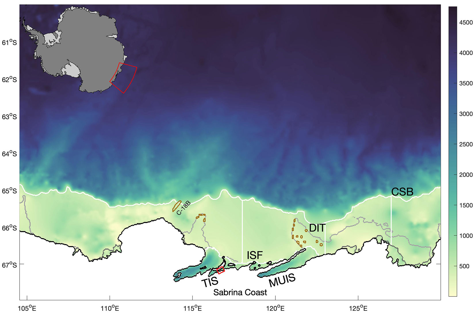
Figure 1 Map of the simulation domain in Wilkes Land along the Sabrina Coast with ocean bathymetry. The coastline is in black, the edge of the (prescribed) landfast sea ice is in grey. Five transects are marked by white lines: the continental shelf break (CSB) and the TIS and MUIS ice shelf fronts (ISF) are irregular contours; three longitudinal white lines across the continental shelf show the three transects from the ice shelf front to the continental shelf break at 118° E, 123° E, and 127° E. The small red square near the TIS shows the location of the inland cavity. Large iceberg C-18B and other grounded icebergs (including those comprising the Dalton Iceberg Tongue, DIT) included in the model are outlined in brown. Figure created with MATLAB Antarctic mapping tools (Greene et al., 2017b) and cmocean (Thyng et al., 2016).

2.3 Forcing data and initial conditions

Considering the periods of tides and eddies, and the cost of the computation, we choose one representative year to carry out the analysis on the role of oceanic eddies and tides on ice shelf basal melt. We selected to run this model with forcing from 2014. This year was chosen after examining the absolute mean values and standard deviation in four forcing components (surface heat flux, surface salt flux, and zonal and meridional wind stresses) over the period 1992 to 2017, which showed that 2014 is the most representative year. (see Supplementary for more details). We used ERA-interim for the reanalysis products as ERA-5 was not available when the simulations were performed.

For the lateral ocean boundary conditions, we use the ECCO2 cube92 solution with 3-day smoothed daily averaged velocity, salinity, and temperatures. Tidal forcing data comes from the global tidal solution Tpxo 6.2 (Egbert and Erofeeva, 2002), with amplitudes and periods for 10 major tidal constituents (M2, S2, N2, K2, K1, O1, P1, Q1, Mm, Mf). We follow Gwyther et al. (2014) and estimated sea ice production by heat and salinity flux derived from Special Sensor Microwave Imager (SSM/I) and Advanced Microwave Scanning Radiometer 2 (AMSR2) data (Tamura et al., 2016; Nihashi et al., 2017). The surface wind stress is derived from daily ERA-Interim reanalysis (ERA-I, 2011).

We spin up the model by repeatedly forcing the model with the 2014 fields as described above for five model years from an initial condition set using the daily forcing of the pseudo-steady state year 1992, and the model rapidly converges. To avoid splitting the austral summer (December, January and February), we ran the model from January 1^st for 14 months, using repeated January and February forcing, and then selecting the continuous 365-day period from March 1^st to February 28^th in the plots shown here.

3 Results and analyses

3.1 Melt rates of TIS and MUIS

During the entire simulation period, the area-averaged basal melt rate of the MUIS is higher than the TIS. The annual mean basal melt rate is 9.7 m yr^-1 for the MUIS and 6.7 m yr^-1 for the TIS (Figure 2). The averaged simulated mass loss for the TIS is 42 Gt yr^-1 and for the MUIS is 52 Gt yr^-1. The area-averaged basal melt rate for the MUIS varies between 8.0 m yr^-1 and 12.9 m yr^-1, and for the TIS varies from 4.8 m yr^-1 to 10.5 m yr^-1. The time series of basal melt rate for both TIS and MUIS show similar trends throughout most of the year. Melt rises from mid-January until the end of May and then declines until around mid-August. From mid-August until mid-September, the basal melt rates of the two ice shelves display an opposing tendency, potentially suggesting interactions between the two ice shelves (Gwyther et al., 2014). From mid-September to mid-January the basal melting of both the ice shelves oscillates within an interval of 3 m yr^-1. There are some transient periods of extremely high melt rate during the year (for example, the spikes on April 1^st, and September 1^st). These spikes are not obviously related to wind forcing or the synoptic weather patterns shown in satellite images of the region (i.e. EOSDIS Worldview; analysis not shown). Hence, we conclude that these spikes are not directly due to surface forcing but instead arise naturally and stochastically within the ocean interactions (see Gwyther et al., 2018 for more discussion of this).

FIGURE 2

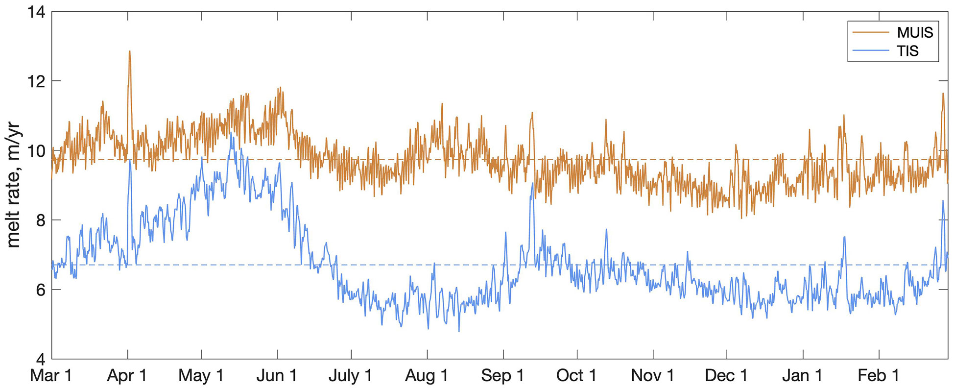
Figure 2 The area-averaged melt rate (m/year) time series for the 2014 simulation year and the annual mean line showed in dashed lines of TIS (in blue), and MUIS (in brown).

3.2 Wavelet coherence

The wavelet coherence (WTC) is a useful measure of the relationships in the time frequency domain between two time series. The WTC is a complex quantity akin to a localized correlation coefficient in time frequency space between two time series along with the localized phase relationship between them. Our hypothesis is that one time series is the proximate driver of changes in the other time series, and the relationship can be investigated by the coherence and phase lag between the two series.

Following Torrence and Webster (1999) and Grinsted et al. (2004) we define the wavelet coherence of two time series as

$\begin{array}{ll}{R}_n^2(s)=\frac{{\left|S(s^{-1}{W}_n^{XY}(s))\right|}^2}{S(s^{-1}{\left|W_n^X(s)\right|}^2)·S(s^{-1}{\left|W_n^Y(s)\right|}^2)},& (1)\end{array}$

where | $W_n^X$(s)|² is the wavelet power from the continuous wavelet transform of a time series (x_n, n=1,…,N) at each scale (that is a measure of the period), s, with uniform time steps δt, which is defined as the convolution of x_n with the scaled and normalized Morlet wavelet. The cross wavelet transform of two time series x_n and y_n is defined as W^XY=W^XW^Y*, where * denotes the complex conjugate. The complex argument arg (W^xy) can be interpreted as the local relative phase between x_n and y_n in time frequency space. S is a smoothing operator, which is defined in technical detail by Grinsted et al. (2004).

The WTC method tests the significance level of correlations in time-frequency space against a random noise null hypothesis using Monte Carlo methods. The key with our data is to modify the null hypothesis from the standard red noise first order autoregressive model applicable in typical climate time series analysis, to a noise spectrum that reflects the actual spectrum of the model data in our experiments, i.e., one with significant power at the various tidal frequencies. So, as the noise background we use an ensemble of WTC generated by 10000 time series with the same mean, standard deviation and randomized phase Fourier decompositions of the two time series. This ensures that the tidal spectrum of the noise surrogates has the same spectral power as the input signals but removes any linear dependencies on the test time series. While the WTC method does not examine any direct measure of causality (such as Granger causality; Granger, 1969), it has some advantages over the kind of strict predictive causality implied in Granger tests and the more ill-defined general concepts of casualty. WTC has been used very widely (Ng and Chan, 2012; Bi et al., 2018; Yadav et al., 2022) because it is useful in describing correlations at multiple periodicities and quantifies phase relationships that can be statistically tested with appropriate noise models.

The WTC between the basal melt rate time series of MUIS and TIS (Figure 3) illustrates the relationship between the basal melting of TIS and MUIS. The arrows indicate the phase differences between the basal melt rate of MUIS and TIS. Yellow areas within the black contour are significant at the 95% level and considered as high coherence between the basal melt rate of two ice shelves. Figure 3 shows a large area of high coherence between the basal melting of two ice shelves over most of the year in the eddy period band (2 to 35 days). This spans the period from March to mid-May as well as from late August to early November. Moreover, → indicates an in-phase (positive) correlation between basal melting of MUIS and TIS, ↗ indicates basal melting of TIS is leading basal melting of MUIS by 45°, and ↘ indicates basal melting of MUIS is leading basal melting of TIS by 45°. From early December to the end of February, the coherent band increases from periods of several days to over a month. Throughout the significant coherence regions in both the tidal and eddy period bands, the phase relation in Figure 3 has arrows generally pointing to the right. This means that both TIS and MUIS melt is in phase with no indication of one ice shelf leading the other. However, from early December to late April and from late August to early November, there is a tendency for the arrows to point more down than up in the eddy band, suggesting that changes in MUIS basal melt rate lead the basal melt rate changes in the TIS with lags varying from 2 to 35 days at a different time of the year.

FIGURE 3

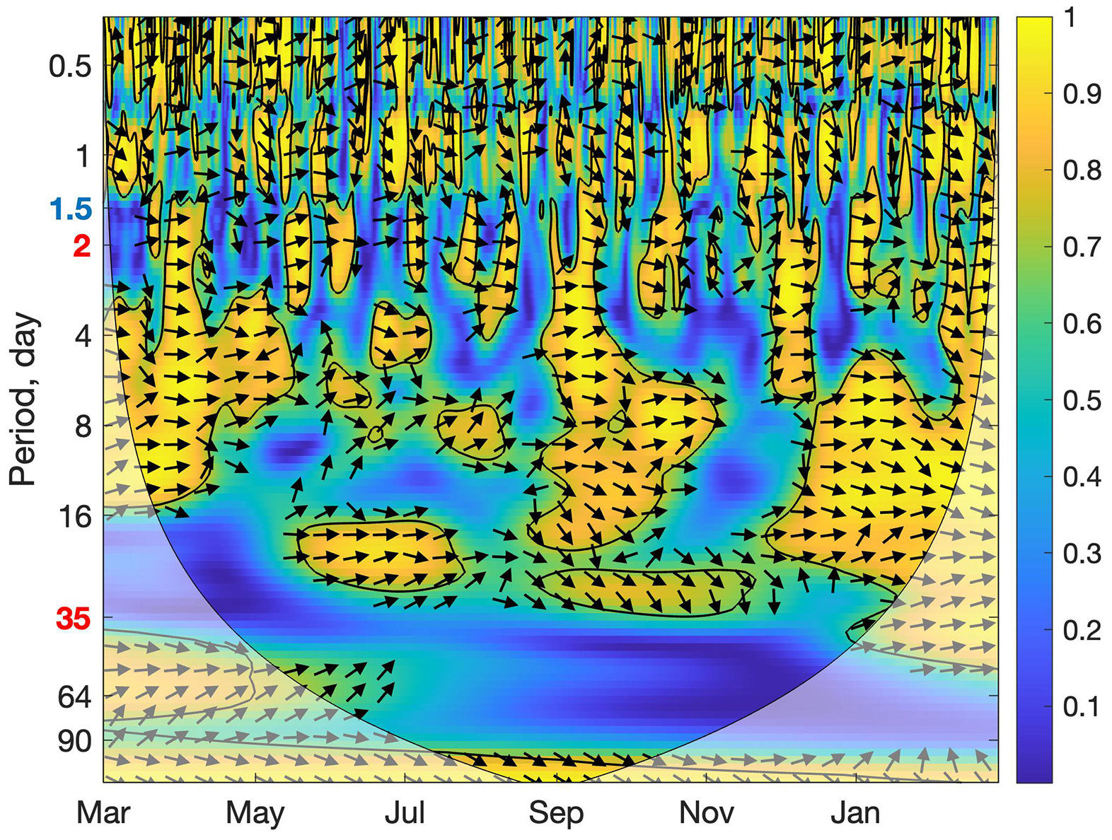
Figure 3 The squared wavelet coherence ${\text{R}}_{\text{ n}}^2$(s) between the area-averaged melt rate time series of MUIS (brown line in Figure 2) and TIS (blue line in Figure 2) in the 2014 simulation year. The low frequency cutoff for tidal periods (1.5 days) is labelled in blue and the lower (35 days) and upper (2 days) frequency cutoffs for the eddy period are labelled in red on the period axis. The color bar indicates a measure of coherence (Eqn. 2). The 95% significance level against a randomized Fourier noise background (see text) is shown as thick contours and the arrows show the relative phase relationship, which is in-phase pointing right, anti-phase pointing left, an arrow pointing straight up means that the TIS leads MUIS melt by 90° at that period, and an arrow pointing down means that TIS lags MUIS by 90°. Moreover, ↗ indicates basal melting of TIS is leading basal melting of MUIS by 45°, and ↘ indicates basal melting of MUIS is leading basal melting of TIS by 45°. The transparent white regions along the edges of the plot represent regions where data boundaries affect the WTC operation, and so represent places where confidence in significance is reduced (Grinsted et al., 2004).

3.3 Spatial patterns of melt

The spatial pattern of the annual average melt rate is shown in Figure 4. Most of the ice shelves are melting during the whole simulation period, except the areas within the black contours, where we simulate basal freezing. Both ice shelves have high basal melt rates in deeper water columns, such as near the southern grounding line (to the south of 67.2° S). Refreezing is present in small quantities in the northwestern portion of the TIS, which corresponds with the likely outflow region of cold ice shelf water (Galton-Fenzi et al., 2012).

FIGURE 4

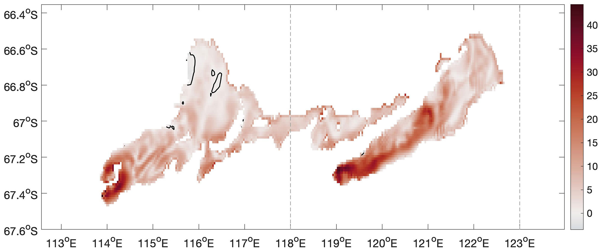
Figure 4 Annual mean basal melt rate (m yr^-1) distribution for the TIS and the MUIS area in the 2014 simulation year. The area within the black contour has negative mean basal melt rate, that is basal freezing is simulated there. Two of the three longitudinal transects (Figure 1) are shown as dashed lines. Figure used cmocean (Thyng et al., 2016).

3.4 What drives basal melting for the two ice shelves?

In general, a westward-flowing coastal current will bring water into ice shelf cavities along their eastern sides, cause the basal melt of the ice shelves and then exit as colder ice shelf water from the western sides (Gwyther et al., 2014). However, on shorter timescales, circulation and heat delivery are likely to be more complex, with eddies and tides playing roles in driving the basal melting. To visualize the relative importance that tides and eddies play in the basal melting of TIS and MUIS, we use five representative transects (Figure 1), including two zonal transects, the ice shelf front (ISF) and the continental shelf break (CSB), and three meridional transects, at 127° E, 123° E, and 118° E that are defined between the ice shelf fronts (or coastlines) and the CSB, marked as vertical white lines in Figure 1. We explore the correlations between the ocean heat transport and sub-ice-shelf melt of TIS and MUIS using WTC at these transects.

3.4.1 WTC results at the three meridional transects

First, we examine the WTC between the area-averaged heat transport time series and area-averaged basal melt rate time series over the 2014 simulation period along the three meridional transects. For the 118° E transect, which is between TIS and MUIS and close to the entrance of TIS, we select the area-averaged basal melt rate of TIS for comparison (Figure 5A). For the 123° E transect, which is the closest to the entrance of the MUIS, we chose both the basal melt rate of TIS and MUIS for comparison (Figures 5B, C). For the 127° E transect, which is the closest to the eastern domain boundary, we chose the area-averaged basal melt rate of MUIS only (Figure 5D). All four WTC plots show strong coherence within the eddy band: between 8 to 32 days from early August to early October, and between 5 to 11 days in early January, which may indicate the presence and impact of a single eddy or an eddy train. Also, arrows within this area of high coherency mostly point down. This implies that at the 118° E and 123° E transects (Figure 5A, B), heat transport leads the basal melting of TIS by a quarter cycle (that is between 2 to 8 days from early August to early October and 1 to 3 days during early January). At the 123° E and 127° E transects (Figures 5C, D), heat transport leads the basal melting of MUIS by similar lags during these months. From these four plots, the strongest eddy contribution along the 118° E transect to the basal melting of TIS (Figure 5A) is from early May to mid-November. Comparing Figures 5B, C, there is a stronger tidal contribution to the basal melting of the MUIS compared to the TIS (i.e., more significant with periods shorter than 1.5 days in Figure 5C) which suggests the stronger and widespread influence of sub-daily and daily tides on the basal melting of MUIS compared to TIS.

FIGURE 5

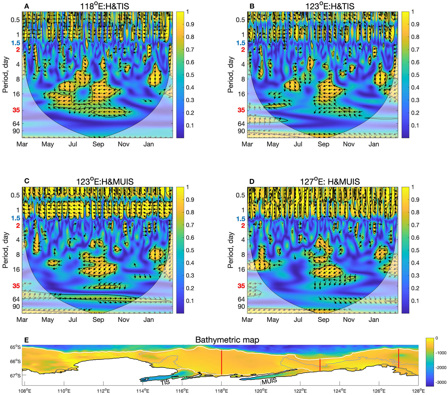
Figure 5 The wavelet coherence between area-averaged heat transport and ice shelf basal melt rate. The ice shelves analysed are identified along with the transect as the title of each subplot which are marked on the location map at the bottom of the figure. Top row are TIS area-averaged basal melt rate time series for 2014 in the 118° E transect (A) and the 123° E transect (B). Middle row are wavelet coherence between area-averaged heat transport and the MUIS area-averaged basal melt rate time series for 2014 in the 123° E transect (C) and the 127° E transect (D). The bottom map (E) shows bathymetric depth and the three longitudinal transects (in red) from the ice shelf front to the continental shelf break.

3.4.2 Contributions from eddies and tides at the three meridional transects

To estimate and compare the eddies and tidal contributions to the basal melt rate of TIS and MUIS, we define the estimated relative contributions from eddies ($C_{eddy}$) and from tides ($C_{tide}$), based on the relative correlations associated with tidal frequencies (< 1.5 days) and at eddy periods (2 to 35 days). We chose 1.5 days rather than say, one day (as chosen by, e.g., Stewart et al., 2018) as the cutoff for representing the tidal period, based on the distribution of the correlations on random WTC maps (e.g., Figures 3, 5) of all the transects. This distinction is somewhat arbitrary as there is some tidal power at longer periods, and it is also possible that some eddies may be longer lived than 1 month (Chelton et al., 2007; Mack et al., 2019), but the key difference in driving force should be captured by any division similar to our choice.

We calculate the WTC between the heat transport time series at each grid cell along the selected transect with the area-averaged melt rate time series. We calculate the sum of the squared correlations ($R_n^2$, eqn. (2)) of the points in time-frequency space within the eddy and tidal period bands, defining $C_{tide}$ and $C_{eddy}$. If $C_{tide}>C_{eddy}$, we assume that tides make a larger contribution to the basal melting at this point and if $C_{tide}<C_{eddy}$ we assume that eddies make a larger contribution to the basal melting.

To understand and estimate the contributions from eddies and tides spatially and with depth, we compare $C_{eddy}$ and $C_{tide}$ on the three longitudinal transects (Figure 6), the ISF (Figure 7) and the CSB (Figure 8). Red indicates eddies dominate the basal melting, and blue indicates tides dominate the basal melting. For the 118° E transect (the first plot of Figure 6), the eddy component of heat transport dominates the basal melting of TIS, though a smaller tidal influenced area is located to the south of 66.8° S. Although the tidal influenced region (in blue) is larger than the eddy influenced area (in red) along the 118° E transect, the eddy dominated regions are closer to the ISF as well as the CSB. The near surface layer is also mostly dominated by eddy-driven processes.

FIGURE 6

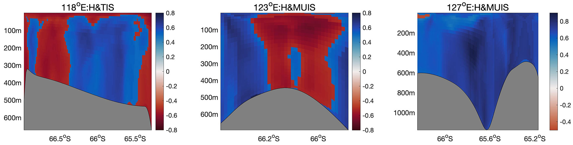
Figure 6 Vertical profiles of $C_{eddy}$ or $C_{tide}$ along various transects marked in Figure 5. Greyed regions are the sea floor. From left to right, the color scale indicates the dominant contributor (red = eddies, blue = tides) to the basal melt rate of TIS or MUIS along 118° E, 123° E and 127° E transects. Figure used cmocean (Thyng et al., 2016).

FIGURE 7

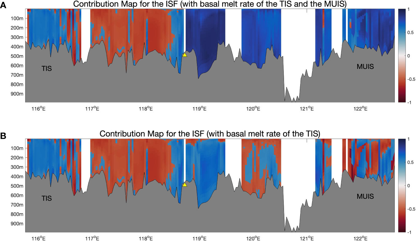
Figure 7 Depth profiles of $C_{eddy}$ (or $C_{tide}$) along the ISF transect, grey regions mark the sea floor topography. Top (A), the estimated contributions from eddies (in red) and tides (in blue) calculated from the WTC between the heat transport at each grid cell and the basal melt rate of TIS (to the west of the yellow triangle area) and the basal melt rate of the MUIS (to the east of the yellow triangle area). Bottom (B), is calculated from the WTC between the heat transport at each grid cell and the basal melt rate of TIS for the whole transect. Figure used cmocean (Thyng et al., 2016).

FIGURE 8

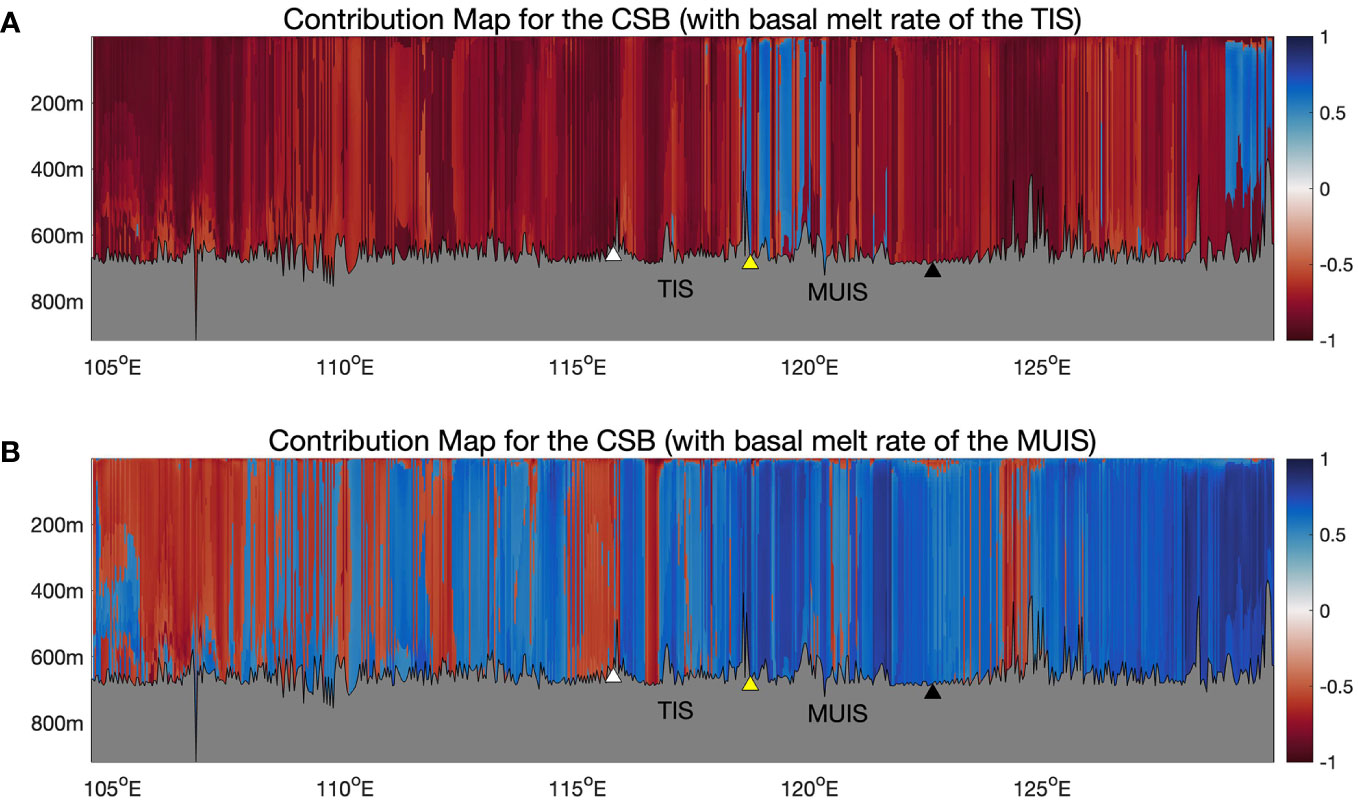
Figure 8 Depth profiles of $C_{eddy}$ (or $C_{tide}$) along the CSB transect, grey regions mark the sea floor topography. Top (A) the estimated contributions from eddies (in red) and tides (in blue) calculated from the WTC between the heat transport at each grid cell and the basal melt rate of TIS. Bottom (B) is calculated from the WTC between the heat transport at each grid cell and the basal melt rate of MUIS. The demarcation point between TIS and MUIS is marked by a yellow triangle. The western boundary of the TIS front is marked by a white triangle (around 115.8° E), and the eastern boundary of the MUIS front is marked by a black triangle (around 122.7° E). Figure used cmocean (Thyng et al., 2016).

The 123° E transect, which is located not far east of the MUIS, is the transect with the shortest distance between the ISF and the CSB among the three. The middle plot of Figure 6 is calculated with heat transport across the 123° E transect and the basal melt rate of MUIS. At this transect, strong tidal influence occurs near the ISF and the CSB, with eddies making the larger contribution on two sides of the rise of the topography (between 65.9° S and 66.3° S), especially for the area shallower than 200 m. We also calculated eddy and tidal contributions to the basal melting of MUIS at a relatively far transect at 127° E (the last plot of Figure 6). It is obvious that tides make the larger contribution over the majority of the region, with only a small near surface region close to the coastline having stronger contributions from eddies. Based on the results of 123° E and 127° E transects, we may state that the basal melting of MUIS is dominated by the tidal component.

3.4.3 Contributions from eddies and tides at the ISF

For the ISF, we can divide the ice shelf area into two parts, the TIS area (to the west of the yellow triangle in Figures 7A, B) and the MUIS area (to the east of the yellow triangle (around 118.7° E)). The TIS area of both plots shows a large red area at the TIS front. The area from 117° E to 118.5° E is mostly in red, which indicates a stronger contribution from eddy components to the basal melting of TIS. The main TIS (from 115.8° E to 116.8° E) is more dominated by tidal processes, while the key inflow region (from 116.4° E to 116.8° E), which is to the eastern side of the main TIS front, shows strong eddy contributions.

For the MUIS front which is to the east of the yellow triangle, we calculated contribution from eddies and tides with the basal melt rate of MUIS (Figure 7A). It is obvious that basal melting of MUIS is mostly dominated by tidal processes. To see how the remote heat transport impacts the basal melting of TIS across the domain, we also calculated the eddy and tidal contributions with the basal melt rate of TIS (Figure 7B). Comparing with Figure 7A, we can see a wide red area spread across the MUIS front. The eddy-dominated area is generally skewed to the left of the main MUIS front (from 121.6° E to 122.6° E) and the area from 119.8° E to 120.5° E. These areas are the outflow region of the MUIS, which means the melt water of MUIS has a strong impact on the basal melting of TIS through eddy processes. This conclusion is consistent with our previous analysis of Figure 3.

3.4.4 Contributions from eddies and tides at the CSB

Lastly, we calculate the contributions from eddy and tidal components of heat transport at the CSB, which is relatively remote from the ice shelves. Figures 8A, B shows $C_{eddy}$ and $C_{tide}$ between heat transport and melt rate time series of TIS and MUIS separately. These two contribution maps intuitively demonstrate the difference in the effect of eddy and tidal components of heat transport at the CSB on the basal melting of the two ice shelves. To explore the eddy and tidal contributions to the basal melting of the two ice shelves, we first analyze the area to the west of the white triangle. In this area, we can clearly see that in Figure 8A, the basal melting of TIS is mainly dominated by the eddy component, while in Figure 8B, the basal melting of MUIS is dominated by the tidal component. For the area between 118.5° E and 120.3° E, eddies and tides alternately dominate the basal melting of TIS. And for the area to the east of 128.9° E, the tidal component has a larger impact on the basal melting of TIS, with only the near bottom and near surface area showing a larger contribution from the eddy component. In the same area in Figure 8B, we can find that the tidal component also dominates the basal melting of MUIS, and the correlation is generally much higher.

The area to the west of the white triangle in both plots reflects the effect of basal melting of the two ice shelves on the heat transport at this area of the CSB since the water masses have exited the ice shelf cavities. Basal melting of TIS influences heat transport at this area mostly through eddy processes, while basal melting of MUIS affects the heat transport in this area through a combination of eddy and tidal processes. In summary, basal melting of TIS is dominated by eddy processes and basal melting of MUIS is dominated by tidal processes. This is consistent with our previous conclusions at three longitudinal transects in Figures 5,  6 and at the ISF in Figure 7.

4 Discussion

In our analyses of eddy and tidal heat transport and basal melting, we have used the single year of 2014 to reduce computational resources and limit output data volume. We selected this year based on its surface heat flux, surface salt flux, and wind stresses in the zonal and meridional directions forcing fields being close to average; hence 2014 can be regarded as a typical year. Other model estimates of ice shelf melt rates for 2014 are limited (Mohajerani et al., 2018; Li et al., 2016), as are direct estimates of mass loss from the Totten and Moscow University glaciers. Recent model work on the Totten Glacier area showed the mean area-averaged basal melt rate from 1995 to 2014 for the TIS is 9.1 ± 4.6 m yr^-1, and for the MUIS is 5.9 ± 5.4 m yr^-1 (Van Achter et al., 2022), which compares well to our results 6.7 m yr^-1 and 9.7 m yr^-1 for TIS and MUIS. Mohajerani et al. (2018) showed the mass balance estimates from two surface mass balance (SMB) models of Totten and Moscow University glaciers for the year 2014 around 100 Gt, which is close to our result (94 Gt). Rignot et al. (2019) calculated the averaged grounding line ice discharge from 2009 to 2017 from Totten Glacier as 71.4 ± 2.6 Gt yr^-1, where the uncertainty is 1 standard error, and for Moscow University Glacier as 47.0 ± 2.1 Gt yr^-1; our model melt rates are 42 and 52 Gt yr^-1 respectively. The MUIS rates are reasonably close, but our TIS estimate are lower than Rignot et al. (2019). However, estimates of ice shelf melt in the complex Totten area can vary by factors of two depending on the methods, with in-situ estimates being much lower than satellite estimates (e.g., Vaňková et al., 2021). Our model estimates are intermediate between the direct and satellite estimates, and perhaps the spread represents more realistic uncertainties in melt than the small variability implied by the Rignot et al. (2019) uncertainty estimate.

We find that the eddy component of heat transport at both ISF and CSB has a larger impact on the basal melting of the TIS, while the tidal component of heat transport dominates the basal melting of the MUIS. The basal melt outflow from MUIS affects the melting mechanism of TIS at eddy periods more than at tidal ones. We raise two following possible reasons why the basal melting of TIS is dominated by eddy processes and the basal melting of MUIS is dominated by tidal processes. Firstly, in our simulation, the water column thickness of TIS is much deeper than MUIS, which leads to larger bathymetric gradients underneath TIS. The presence of an inland cavity (Figure 1) and the complex geometry of the grounded ice area show that the TIS terrain is convoluted. The locally steep gradients and complex terrain of the TIS cavity seem to promote more transport of heat into the grounding zone of TIS by local mesoscale eddies than higher frequency tidal motions, in an analogous way to lower frequency sound suffering less loss than high frequencies in convoluted geometrical settings. The mesoscale physical processes can generate more local mixing than tides. Secondly, we conjecture that this phenomenon is closely related to the westward flowing Antarctic Coastal Current. TIS is located to the west of MUIS and hence is downstream area of MUIS. Figure 3 shows there is high coherence between the basal melting of TIS and MUIS. MUIS meltwater flows westward and intrudes into the TIS cavity. This cold dense water can enhance the local mixing of water mass, hence promote more eddies to transport warm water into the TIS cavity and promote the basal melting. Gwyther et al. (2014) note that the Antarctic Slope Current can flow southward into the Totten Basin and bring warm current into the TIS cavity. Hence, we propose that complex circulation near the TIS area may provide favorable conditions for the formation of eddies.

Contributions from eddies are stronger near the ISF and the CSB along the 118° E transect, which could be due to the sudden deepening of the topography towards the southern and northern boundary in Figure 6. Mizobata et al. (2020) confirmed the existence of a large scale cyclonic eddy train near the Sabrina Coast (the coast of Wilkes Land between 115°33’ E and 122°05’ E), which plays a critical role in transporting warm CDW onto the continental shelf, then intruding into the cavities and cause the basal melting. For the 123° E transect to the east of the MUIS, where the eddies may not be as dense, tidal components make larger contributions near the ISF and the CSB. Studies confirm that tidal fluctuations could enhance the cross-slope exchange, which would contribute to the poleward heat transport at the continental shelf break (Padman et al., 2009; Mack et al., 2017). The ISF has similar features as the CSB.

Applying the WTC method over longer time scales, even spanning some decades is possible, although data volume becomes an issue. Multi-decadal variability driven from the Pacific Ocean is known to play important roles in the pumping of meltwater onto the continental shelf in the Amundsen Sea sector (Holland et al., 2019). Many features of the melt rates are unexplained, such as the large spikes seen sporadically e.g., Figure 2 on April 1^st and September 1^st. These large events have power over very broad bands in the WTC as might be expected from a delta function. Assuming that the spikes are not purely numerical model artifacts, the obvious proximate causes would be an intense local storm, but this interpretation is not supported by available satellite and weather data in the region. However, a more distal source would exhibit frequency dispersion and peak broadening in the wavelet plot from diffusive processes in the ocean. Information on wavelet coherence at longer periods would provide better statistical evidence that might reveal mechanisms for these spikes, as well as resolving the importance of longer-term oceanic variability in ice shelf melt.

In this model we do not include a frazil ice parameterization, though we acknowledge the importance of frazil ice in refreezing. However, we expect that it is not a major consideration for the Totten ice shelf, as the warm ocean cavity conditions broadly inhibits marine refreezing (Gwyther et al., 2015). In a cooler cavity environment like the Amery Ice Shelf, frazil is certainly an important component that should not be neglected (Galton-Fenzi et al., 2012).

Understanding the role of the ocean is important for estimating the mass loss of the ice sheet. Variability of the Totten Glacier has been confirmed to be primarily driven by oceanic processes (Roberts et al., 2017). The simulations and insights from this work would be more comprehensive if done using a fully coupled ice sheet-ocean model to simulate the oceanic environment and the evolution of the ice shelf, for example combining the ROMS and Elmer/Ice using the Framework for Ice Sheet-Ocean Coupling (Gladstone et al., 2021). It would then be feasible to make inferences directly on the role of changing oceanic forcing on the sea level rise contribution for these ice shelf catchments.

5 Conclusions

We apply a three-dimensional eddy-resolving oceanic model (ROMS) at a resolution better than 2 km, to simulate the Wilkes Land region and then used a novel application of the wavelet coherence method to estimate the contributions from eddies and tides to the basal melting of TIS and MUIS. During the 2014 simulation period, the area-averaged basal melting of the MUIS is higher than the TIS. The WTC method shows that strong coherence exits between ice shelf melt at the two ice shelves throughout almost the whole simulation year, which confirms strong interaction between the two ice shelves.

We look at the spatial pattern of contributions from eddies and tides to ocean heat transport based on the wavelet decomposition and coherence of ice shelf melt and heat transport. Our analysis shows that basal melting of the TIS is dominated by the eddy processes, while the basal melting of the MUIS is more controlled by tidal processes. For the 118° E transect, which lies equidistant between the TIS and MUIS, eddies drive heat flux transport used in TIS basal melting from near the ISF and the CSB, while tidal processes make larger contributions over the continental shelf area. For the 123° E transect, to the east of the MUIS, the influence from eddies and tides are almost opposite. We find stronger tidal contributions to the basal melting of the MUIS resulting from the ISF and the CSB, while for the continental shelf region, the eddy component of the ocean heat transport dominates the basal melting. For the easternmost transect at 127° E, the tidal component of the ocean heat transport dominates the basal melting of the TIS and the MUIS. The eddy processes make larger contributions near the ISF and the CSB area where more eddies are observed and where the western dense shelf water outflows. Tidal processes dominate the basal melting to the east of the MUIS which is the inflow area of the two ice shelves.

These results are likely dependent on the accuracy of the topography of bedrock and the ice draft because the relative impact of tides and eddies will depend on the geometry of the cavities the heat is transported through. In this respect, more field data collected near the ISF of TIS and MUIS and the CSB of Wilkes Land region to compare with model results may provide wider confirmation of sub-shelf bathymetry. Perhaps even more useful would be a comprehensive coupled model with ocean and ice shelf components that could be driven by realistic variability expected for various future scenarios.

Data availability statement

The raw data supporting the conclusions of this article will be made available by the authors, without undue reservation.

Author contributions

YX modified the model parameters, ran the simulation, analyzed the model output and plotted the figures and composed the paper. DG designed and assisted in the model set up, input data, the analysis of the results, and editing of the text. BG-F assisted in designing the idea of the paper, offering suggestions with the analysis and results. JM contributed the idea of the WTC method, assisted in modifying the MATLAB codes, analysis of the results and editing the text. EC assisted with the MATLAB codes, participated in the discussion of the results and offered suggestions. AF offered fast ice data and participated in the discussion of the results. All authors contributed to the article and approved the submitted version.

Funding

This research has been supported by the National Key Research and Development Program of China (grant no. 2021YFB3900105), and Finnish Academy COLD Consortium (grant no. 322430). YX was supported by the Chinese Scholarship Consulate during her abroad study at the University of Tasmania.

Acknowledgments

We thank the Chinese Scholarship Consulate and Chinese MOST grant 2015CB953602 for financial support. We are grateful for the support from the University of Tasmania. This project received grant funding from the Australian Government as part of the Antarctic Science Collaboration Initiative program.

Conflict of interest

The authors declare that the research was conducted in the absence of any commercial or financial relationships that could be construed as a potential conflict of interest.

Publisher’s note

All claims expressed in this article are solely those of the authors and do not necessarily represent those of their affiliated organizations, or those of the publisher, the editors and the reviewers. Any product that may be evaluated in this article, or claim that may be made by its manufacturer, is not guaranteed or endorsed by the publisher.

Supplementary material

The Supplementary Material for this article can be found online at: https://www.frontiersin.org/articles/10.3389/fmars.2023.1159353/full#supplementary-material

References

Arndt J. E., Schenke H. W., Jakobsson M., Nitsche F. O., Buys G., Goleby B., et al. (2013). The international bathymetric chart of the southern ocean (IBCSO) version 1.0 - a new bathymetric compilation covering circum-Antarctic water. Geophys. Res. Lett. 40, 3111–3117. doi: 10.1002/grl.50413

CrossRef Full Text | Google Scholar

Bi S., Qu Y., Bi S., Wu W., Jiang T. (2018). Multi-scale impacts of the Pacific SST and PDO on the summer precipitation of North-Central China from 1870 to 2002. Theor. Appl. Climatol. 132, 953–863. doi: 10.1007/s00704-017-2145-2

CrossRef Full Text | Google Scholar

Chelton D. B., Schlax M. G., Samelson R. M., de Szoeke R. A. (2007). Global observations of large oceanic eddies. Geophys. Res. Lett. 34, L15606. doi: 10.1029/2007GL030812

CrossRef Full Text | Google Scholar

Couto N., Martinson D. G., Kohut J., Schofield O. (2017). Distribution of upper circumpolar deep water on the warming continental shelf of the West Antarctic peninsula. J. Geophys. Res. Oceans 122, 5306–5315. doi: 10.1002/2017JC012840

CrossRef Full Text | Google Scholar

Dinniman M. S., Klinck J. M., Smith W. O. (2003). Cross-shelf exchange in a model of the Ross Sea circulation and biogeochemistry. Deep Sea Res. Part II: Topical Stud. Oceanogr 50 (22-26), 3103–3120. doi: 10.1016/j.dsr2.2003.07.011

CrossRef Full Text | Google Scholar

Egbert G. D., Erofeeva S. Y. (2002). Efficient inverse modelling of barotropic ocean tides. J. Atmos. Oceanic Tech. 19 (2), 183–204. doi: 10.1175/1520-0426(2002)019<0183:EIMOBO>2.0.CO;2

CrossRef Full Text | Google Scholar

EOSDIS Worldview. Available at: https://worldview.earthdata.nasa.gov/.

Google Scholar

ERA-I (2011) The ERA-interim reanalysis. European centre for medium-range weather forecasts (ECMWF). Available at: http://apps.ecmwf.int/datasets/data/interim-full-daily (Accessed 15 February 2016).

Google Scholar

Ferraccioli F., Armadillo E., Jordan T., Bozzo E., Corr H. (2009). Aeromagnetic exploration over the East Antarctic ice sheet: A new view of the Wilkes subglacial basin. Tectonophysics 478 (1-2), 62–77. doi: 10.1016/j.tecto.2009.03013

CrossRef Full Text | Google Scholar

Fraser A. D., Massom R., Michael K. J., Galton-Fenzi B. K., Lieser J. L. (2012). East Antarctic Landfast Sea ice distribution and variability 2000-08. J. Climate 25, 1137–1156. doi: 10.1175/JCLI-D-10-05032.1

CrossRef Full Text | Google Scholar

Fraser A. D., Massom R. A., Ohshima K. I., Willmes S., Kappes P. J., Cartwright J., et al. (2020). High-resolution mapping of circum-Antarctic landfast sea ice distribution 2000-2018. Earth Syst. Sci. Data 12, 2987–2999. doi: 10.5194/essd-12-2987-2020

CrossRef Full Text | Google Scholar

Fretwell P., Pritchard H. D., Vaughan D. G., Bamber J. L., Barrand N. E., Bell R., et al. (2013). Bedmap2: improved ice bed, surface and thickness datasets for Antarctica. Cryosphere 7, 375–393. doi: 10.5194/tc-7-3752013

CrossRef Full Text | Google Scholar

Galton-Fenzi B. K., Hunter J. R., Coleman R., Marsland S. J., Warner R. C. (2012). Modeling the basal melting and marine ice accretion of the amery ice shelf. J. Geophys. Res. 117, C09031. doi: 10.1029/2012JC008214

CrossRef Full Text | Google Scholar

Giles A. B., Massom R. A., Lytle V. I. (2008). Fast-ice distribution in East Antarctica during 1997 and 1999 determined using RADARSAT data. J. Geophys. Res. 113, C02S14. doi: 10.1029/2007JC004139

CrossRef Full Text | Google Scholar

Gladstone R. M., Galton-Fenzi B., Gwyther D. E., Zhou Q., Hattermann T., Zhao C., et al (2021). The framework for ice sheet-ocean coupling (FISOC) V1.1. Geosci. Model Dev. 14, 889–905. doi: 10.5194/gmd-14-889-2021

CrossRef Full Text | Google Scholar

Graham J. A., Dinniman M. S., Klinck J. M. (2016). Impact of model resolution for on-shelf heat transport along the West Antarctic peninsula. J. Geophys. Res. Oceans 121, 7880–7897. doi: 10.1002/2016JC011875

CrossRef Full Text | Google Scholar

Granger C. W. J. (1969). Investigating causal relations by econometric models and cross spectral methods. Econometrica 37, 424–438. doi: 10.2307/1912791

CrossRef Full Text | Google Scholar

Greenbaum J. S., Blankenship D. D., Young D. A., Richter T. G., Roberts J. L., Aitken A. R. A., et al. (2015). Ocean access to a cavity beneath totten glacier in East Antarctica. Nat. Geosci. 8 (4), 294–298. doi: 10.1038/ngeo2388

CrossRef Full Text | Google Scholar

Greene C. A., Blankenship D. D., Gwyther D. E., Silvano A., van Wijk E. (2017a). Wind causes totten ice shelf melt and acceleration. Sci. Adv. 3 (11), e1701681. doi: 10.1126/sciadv.1701681

PubMed Abstract | CrossRef Full Text | Google Scholar

Greene C. A., Gwyther D. E., Blankenship D. D. (2017b). Antarctic Mapping tools for Matlab. Comput. Geosci. 104, 151–157. doi: 10.1016/j.cageo.2016.08.003

CrossRef Full Text | Google Scholar

Greene C. A., Young D. A., Gwyther D. E., Galton-Fenzi B. K., Blankenship D. D. (2018). Seasonal dynamics of totten ice shelf controlled by sea ice buttressing. Cryosphere 12, 2869–2882. doi: 10.5194/tc-12-2869-2018

CrossRef Full Text | Google Scholar

Grinsted A., Moore J. C., Jevrejeva S. (2004). Application of the cross wavelet transform and wavelet coherence to geophysical time series. Nonlin. Processes Geophys. 11, 561–566. doi: 10.5194/npg-11-561-2004

CrossRef Full Text | Google Scholar

Gudmundsson G. H., Krug J., Durand G., Favier L., Gagliardini O. (2012). The stability of grounding lines on retrograde slopes. Cryosphere 6, 1497–1505. doi: 10.5194/tc-6-1497-2012

CrossRef Full Text | Google Scholar

Gwyther D. E., Galton-Fenzi B. K., Dinniman M. S., Roberts J. L., Hunter J. R. (2015). The effect of basal friction on melting and freezing in ice shelf-ocean models. Ocean Modellling 95, 38–52. doi: 10.1016/j.ocemod.2015.09.004

CrossRef Full Text | Google Scholar

Gwyther D. E., Galton-Fenzi B. K., Hunter J. R., Roberts J. L. (2014). Simulated melt rates for the totten and Dalton ice shelves. Ocean Sci. 10, 267–279. doi: 10.5194/os-10-267-2014

CrossRef Full Text | Google Scholar

Gwyther D. E., O'Kane T. J., Galton-Fenzi B. K., Monselesan D. P., Greenbaum J. S. (2018). Intrinsic processes drive variability in basal melting of the totten glacier ice shelf. Nat. Commun. 9, 3141. doi: 10.1038/s41467-018-05618-2

PubMed Abstract | CrossRef Full Text | Google Scholar

Hattermann T., Smedsrud L. H., Nøst O. A., Lilly J. M., Galton-Fenzi B. K. (2014). Eddy-resolving simulations of the fimbul ice shelf cavity circulation: Basal melting and exchange with open ocean. Ocean Model. 82, 28–44. doi: 10.1016/j.ocemod.2014.07.004

CrossRef Full Text | Google Scholar

Hirano D., Mizobata K., Sasaki H., Murase H., Tamura T., Aoki S. (2021). Poleward eddy-induced warm water transport across a shelf break off totten ice shelf, East Antarctica. Commun. Earth Environ. 2, 153. doi: 10.1038/s43247-021-00217-4

CrossRef Full Text | Google Scholar

Holland P. R., Bracegirdle T. J., Dutrieux P., Jenkins A., Steig E. J. (2019). West Antarctic Ice loss influenced by internal climate variability and anthropogenic forcing. Nat. Geosci. 12, 718–724. doi: 10.1038/s41561-019-0420-9

CrossRef Full Text | Google Scholar

Holland D. M., Jenkins A. (1999). Modeling thermodynamic ice-ocean interactions at the base of an ice shelf. J. Phys. Oceanogr. 29, 1787–1800. doi: 10.1175/15200485(1999)029<1787:MTIOIA>2.0.CO;2

CrossRef Full Text | Google Scholar

Hughes T. (1973). Is the west Antarctic ice sheet disintegrating? J. Geophys. Res. 78 (33), 7884–7910. doi: 10.1029/JC078i033p07884

CrossRef Full Text | Google Scholar

Jackson L. P., Jevrejeva S. (2016). A probabilistic approach to 21st century regional sea level projections using RCP and high-end scenarios. Global Planet. Change 146, 179–189. doi: 10.1016/j.gloplacha.2016.10.006

CrossRef Full Text | Google Scholar

Jacobs S. S., Helmer H. H., Doake C. S. M., Jenkins A., Frolich R. M. (1992). Melting of ice shelves and the mass balance of Antarctica. J. Glaciol. 38 (130), 375–387. doi: 10.3189/S0022143000002252

CrossRef Full Text | Google Scholar

Klinck J. M., Dinniman M. S. (2010). Exchange across the shelf break at high southern latitudes. Ocean Sci. 6, 513–524. doi: 10.5194/os-6-513-2010

CrossRef Full Text | Google Scholar

Kusahara K., Hasumi H. (2013). Modeling Antarctic ice shelf responses to future climate changes and impacts on the ocean. J. Geophys. Res. Oceans 118, 2454–2475. doi: 10.1002/jgrc.20166

CrossRef Full Text | Google Scholar

Large W. G., McWilliams J. C., Doney S. C. (1994). Oceanic vertical mixing: A review and model with a nonlocal boundary layer parameterization. Rev. Geophys. 32, 363–403. doi: 10.1029/94RG01872

CrossRef Full Text | Google Scholar

Li X., Rignot E., Mouginot J., Scheuchl B. (2016). Ice flow dynamics and mass loss of Totten Glacier, East Antarctica, from 1989 to 2015. Geophys. Res. Lett. 43, 6366–6373. doi: 10.1002/2016GL069173

CrossRef Full Text | Google Scholar

Lieser J. L., Massom R. A., Heil P. (2014). Sea Ice reports for the season 2013-2014 (Hobart, Tasmania: Antarctic Climate & Ecosystems Cooperative Research Centre). doi: 10.4226/77/5b1880a782a63

CrossRef Full Text | Google Scholar

Lieser J. L., Massom R. A., Heil P. (2015). Sea Ice reports for the Antarctic shipping season 2014-2015 (Hobart, Tasmania: Antarctic Climate & Ecosystems Cooperative Research Centre). doi: 10.4226/77/5b187b7182a62

CrossRef Full Text | Google Scholar

Liu Y., Moore J. C., Cheng X., Gladstone R. M., Bassis J. N., Liu H., et al. (2015). Ocean-driven thinning enhances iceberg calving and retreat of Antarctic ice shelves. Proc. Natl. Acad. Sci. 112 (11), 3263–3268. doi: 10.1073/pnas.1415137112

CrossRef Full Text | Google Scholar

Mack S. L., Dinniman M. S., Klinck J. M., McGillicuddy D. J. Jr., Padman L. (2019). Modeling ocean eddies on antarctica's cold water continental shelves and their effects on ice shelf basal melting. J. Geophys. Res. Oceans 124, 5067–5084. doi: 10.1029/2018JC014688

CrossRef Full Text | Google Scholar

Mack S. L., Dinniman M. S., McGillicuddy D. J., Sedwick P. N., Klinck J. M. (2017). Dissolved iron transport pathways in the Ross Sea: Influence of tides and horizontal resolution in a regional ocean model. J. Mar. Syst. 166, 73–86. doi: 10.1016/j.jmarsys.2016.10.008

CrossRef Full Text | Google Scholar

Mizobata K., Shimada K., Aoki S., Kitade Y. (2020). The cyclonic eddy train in the Indian ocean sector of the southern ocean as revealed by satellite radar altimeters and in situ measurements. J. Geophy. Res. Oceans 125, e2019JC015994. doi: 10.1029/2019JC015994

CrossRef Full Text | Google Scholar

Mohajerani Y., Velicogna I., Rignot E. (2018). Mass loss of totten and Moscow university glaciers, East Antarctica, using regionally optimized GRACE mascons. Geophys. Res. Lett. 45, 7010–7018. doi: 10.1029/2018GL078173

CrossRef Full Text | Google Scholar

Moore J. C., Grinsted A., Zwinger T., Jevrejeva S. (2013). Semi-empirical and process-based global sea level projections. Rev. Geophys. 51, 484–552. doi: 10.1002/rog.20015

CrossRef Full Text | Google Scholar

Ng E. K. W., Chan J. C. L. (2012). Geophysical applications of partial wavelet coherence and multiple wavelet coherence. J. Atmos. Oceanic Technol. 29 (12), 1845–1853. doi: 10.1175/JTECH-D-12-00056.1

CrossRef Full Text | Google Scholar

Nihashi S., Ohshima K. I., Tamura T. (2017). Sea-Ice production in Antarctic coastal polynyas estimated from AMSR2 data and its validation using AMSR-e and SSM/I-SSMIS data. (in IEEE). J. Sel. Topics App. Earth Obs. Remote Sens. 10 (9), 3912–3922. doi: 10.1109/JSTARS.2017.2731995

CrossRef Full Text | Google Scholar

Nitsche F. O., Porter D., Williams G., Cougnon E. A., Fraser A. D., Correia R., et al. (2017). Bathymetric control of warm ocean water access along the East Antarctic margin. Geophys. Res. Lett. 44, 8936–8944. doi: 10.1002/2017GL074433

CrossRef Full Text | Google Scholar

Padman L., Howard S. L., Orsi A. H., Muench R. D. (2009). Tides of the northwestern Ross Sea and their impact on dense outflows of Antarctic bottom water. Deep Sea Res. Part II: Topical Stud. Oceanogr 56 (13), 818–834. doi: 10.1016/j.dsr2.2008.10.026

CrossRef Full Text | Google Scholar

Padman L., Siegfried M. R., Fricker H. A. (2018). Ocean tide influences on the Antarctic and Greenland ice sheets. Rev. Geophys. 56, 142–184. doi: 10.1002/2016RG000546

CrossRef Full Text | Google Scholar

Pattyn F., Ritz C., Hanna E. (2018). The Greenland and Antarctic ice sheets under 1.5 °C global warming. Nat. Climate Change 8, 1053–1061. doi: 10.1038/s41558-018-0305-8

CrossRef Full Text | Google Scholar

Pritchard H. D., Ligtenberg S. R. M., Fricker H. A., Vaughan D. G., van den Broeke M. R., Padman L. (2012). Antarctic Ice-sheet loss driven by basal melting of ice shelves. Nature 484, 502–505. doi: 10.1038/nature10968

PubMed Abstract | CrossRef Full Text | Google Scholar

Rignot E., Jacobs S., Mouginot J., Scheuchl B. (2013). Ice-shelf melting around Antarctica. Science 341 (6143), 266–270. doi: 10.1126/science.1235798

PubMed Abstract | CrossRef Full Text | Google Scholar

Rignot E., Mouginot J., Scheuchl B. (2016). MEaSURES Antarctic grounding line from different satellite radar interferometry, version 2 (Boulder, Colorado USA: NASA National Snow and Ice Data Center Distributed Active Archive Center). doi: 10.5067/IKBWW4RYHF1Q

CrossRef Full Text | Google Scholar

Rignot E., Mouginot J., Scheuchl B., van den Broeke M., van Wessem M. J., Morlighem M. (2019). Four decades of Antarctic ice sheet mass balance from 1979-2017. Proc. Natl. Acad. Sci. 116 (4), 1095–1103. doi: 10.1073/pnas.18128883116

CrossRef Full Text | Google Scholar

Roberts J. L., Warner R. C., Young D., Wright A., van Ommen T. D., Blankenship D. D., et al. (2011). Refined broad-scale sub-glacial morphology of aurora subglacial basin, East Antarctica derived by a ice-dynamics-based interpolation scheme. Cryosphere 5, 551–560. doi: 10.5194/tc-5-551-2011

CrossRef Full Text | Google Scholar

Roberts J. L., Galton-Fenzi B. K., Paolo F. S., Donnelly C. B., Gwyther D. E., Padman L., et al (2017). Ocean forced variability of Totten Glacier mass loss. Geol. Soc. Spec. Publ. 461, 175–186. doi: 10.1144/SP461.6

CrossRef Full Text | Google Scholar

Rott H., Rack W., Skvarca P., Angelis H. (2002). Northern Larsen ice shelf, Antarctica: Future retreat after collapse. Ann. Glaciol. 34, 277–282. doi: 10.3189/172756402781817716

CrossRef Full Text | Google Scholar

Schaffer J., Timmermann R., Arndt J. E., Kristensen S. S., Mayer C., Morlighem M., et al. (2016). A global high-resolution data set of ice sheet topography, cavity geometry and ocean bathymetry. Earth Sys. Sci. Data 8, 543–557. doi: 10.5194/essd-2016-3

CrossRef Full Text | Google Scholar

Schoof C. (2007). Ice sheet grounding line dynamics: Steady states, stability and hysteresis. J. Geophys. Res. 112, F03S28. doi: 10.1029/2006JF000664

CrossRef Full Text | Google Scholar

Shchepetkin A. F., McWilliams J. C. (2005). The regional oceanic modeling system (ROMS): a split-explicit, free-surface, topography-following-coordinate oceanic model. Ocean Model. 9, 347–404. doi: 10.1016/j.ocemod.2004.08.002

CrossRef Full Text | Google Scholar

Silvano A., Rintoul S. R., Herraiz-Borreguero L. (2016). Ocean-ice shelf interaction in East Antarctica. Oceanography 29 (4), 130–143. doi: 10.5670/oceanog.2016.105

CrossRef Full Text | Google Scholar

Silvano A., Rintoul S. R., Penã-Molino B., Williams G. D. (2017). Distribution of water masses and meltwater on the continental shelf near the totten and Moscow university ice shelves. J. Geophys. Res. Oceans 122, 2050–2068. doi: 10.1002/2016JC012115

CrossRef Full Text | Google Scholar

Stewart A. L., Klocker A., Menemenlis D. (2018). Circum-Antarctic shoreward heat transport derived from an eddy- and tide-resolving simulation. Geophys. Res. Lett. 45, 834–845. doi: 10.1002/2017GL075677

CrossRef Full Text | Google Scholar

Tamura T., Ohshima K. I., Fraser A. D., Williams G. D. (2016). Sea Ice production variability in Antarctic coastal polynyas. J. Geophys. Res. Oceans 121, 2967–2979. doi: 10.1002/2015JC011537

CrossRef Full Text | Google Scholar

Thyng K. M., Greene C. A., Hetland R. D., Zimmerle H. M., DiMarco S. F. (2016). True colors of oceanography: Guidelines for effective and accurate colormap selection. Oceanography 29 (3), 9–13. doi: 10.5670/oceanog.2016.66

CrossRef Full Text | Google Scholar

Torrence C., Webster P. (1999). Interdecadal changes in the ESNO monsoon system. J. Clim. 12, 2679–2690. doi: 10.1175/1520-0442(1999)012<2679:ICITEM>2.0CO;2

CrossRef Full Text | Google Scholar

Van Achter G., Fichefet T., Goose H., Moreno-Chamarro E. (2022). Influence of fast ice on future ice shelf melting in the totten glacier area, East Antarctica. Cryosphere 16, 4745–4761. doi: 10.5194/tc-16-4745-2022

CrossRef Full Text | Google Scholar

Vaňková I., Cook S., Winberry J. P., Nicholls K. W., Galton-Fenzi B. K. (2021). Deriving melt rates at a complex ice shelf base using in situ radar: Application to totten ice shelf. Geophys. Res. Lett. 48, e2021GL092692. doi: 10.1029/2021GL092692

CrossRef Full Text | Google Scholar

Yadav J., Kumar A., Srivastava A., Mohan R. (2022). Sea Ice variability and trends in the Indian ocean sector of Antarctica: Interaction with ENSO and SAM. Environ. Res. 212, Part D. doi: 10.1016/j.envres.2022.113481

CrossRef Full Text | Google Scholar