 Ronald Raulefs
 Miguel A. Bellido-Manganell1
 Armin Dammann
 Michael Walter
 Wei Wang
94% of researchers rate our articles as excellent or good
Learn more about the work of our research integrity team to safeguard the quality of each article we publish.
Find out more
ORIGINAL RESEARCH article
Front. Mar. Sci., 06 November 2023
Sec. Ocean Observation
Volume 10 - 2023 | https://doi.org/10.3389/fmars.2023.1158524
This article is part of the Research TopicMaritime Broadband Communications and NetworkingView all 7 articles
This paper presents a geometric stochastic channel model designed for analyzing maritime communication and navigation services between moving ships using the C-band or sub-6 GHz spectrum, which aligns with the focus of emerging 5G networks on land. The channel model is validated through channel measurements conducted both on the sea and land. A software tool has been developed to integrate and analyze these measurements, which is included with this publication. The main challenge in developing the channel model for maritime services lies in the dynamic nature of the sea surface, leading to constantly changing reflection conditions due to varying reflectors and scatterers on the water. Additionally, the motion conditions of the transmitter and receiver on ships change in all three dimensions, depending on the sea state. To address these complexities, data from several measurement campaigns in diverse areas were collected. The analysis involved examining the propagation conditions over the sea with variations in sea surface roughness, antenna heights, and used bandwidths. Moreover, additional propagation conditions over nearby land were also taken into account. The study demonstrates that the changing antenna height on the ship, influenced by sea conditions, significantly affects the reflection and scattering conditions. The research aims to develop reliable, high-data rate, and broadband marine communication systems. Therefore, a measurement bandwidth of 120MHz was employed to derive the propagation model. This model not only offers absolute timing information but can also be used for time-based ranging or positioning systems. The proposed geometric stochastic channel model provides valuable insights into the complex maritime communication and navigation environment. By accounting for the continuously evolving sea surface and its impact on antenna height, the model offers a robust framework for studying and optimizing marine communication systems. The availability of a software tool integrating real-world measurements further enhances the usability and practicality of the channel model for future maritime communication research and deployment.
The shipping industry has identified the need to increase demands for broadband communications for various applications, such as remotely controlled vessels by pilots or observation data of marine sensor networks. In contrast to the shore-to-ship connection, the ship-to-ship (S2S) connection is a rather unexplored area that is crucial for ad hoc networks that are historically typical in the marine world. A maritime network demands different requirements compared to terrestrial communication networks on land. The distance between the vessels and the shore station is significantly larger, and the environment including the surface is constantly changing.
In cellular mobile radios, a dense network with small coverage areas of base stations that focus on a limited number of mobile users enables low latency and high data rates. Base station antenna arrays allow directing antenna beams to mobile users in a more static or predictable environment to limit user and cell interference. Mobile users move indoors at limited speeds and in known areas. In contrast, in maritime communications, the classic maritime requirements, such as range and one-dimensional cell structures, and a time-varying moving sea surface are not well served by the land-based cellular network infrastructure. In maritime networks, steered antennas on the shore and adaptive antenna arrays on the ship with significant antenna gains compared to omnidirectional antennas are applied to increase the range.
In Korea, a maritime LTE system is being rolled out (Jo and Shim, 2019) with a focus on long-distance land-to-ship links with data rates in excess of 10 Mbit/s. The maritime LTE system addresses the concerns of long-range communications beyond 100 km. In addition, the fifth generation of cellular mobile systems, 5G, has identified the need for maritime communications to support high data rates as addressed by cyber-physical control applications in TS 22.104 3rd Generation Partnership Project (3GPP) (2023) and maritime services in TS 22.119 3rd Generation Partnership Project (3GPP) (2022) for the 3GPP systems.
Accidents in the shipping industry (Allianz, 2022; Paolo et al., 2021) have a significant impact and are mostly caused by the human element. Lack of situational awareness is an underlying factor in human error and violations leading to collisions, groundings, and occupational accidents. Situational awareness (Forti et al., 2022; Thombre et al., 2022) uses communication links that allow a remotely controlled vessel to sense its surroundings through a rich set of sensors to navigate more reliably and safely. Maritime networks (Du et al., 2021; Guan et al., 2021) are expected to deliver improvements in several areas of the maritime industry, such as offshore oil exploration, aquaculture and fishing, law enforcement, and the success rate of search and rescue operations following maritime accidents. All of this relies on a detailed understanding of radio propagation to detect anomalies and the need to communicate such sensor information for a decision-driven process (Forti et al., 2022).
The most critical aspect of maritime shipping is navigation, which is provided by the global navigation satellite system (GNSS). Compared to terrestrial systems, where there is an alternative navigation system to GNSS based on WiFi or cellular networks on the open sea, the mariners are solely dependent on their eyesight (Sadlier et al., 2017). Therefore, an onboard contingency navigation system based on maritime communication networks would increase the resilience of navigation at sea. A joint communication and navigation maritime channel model must take into account the absolute delay and signal strength of each relevant multipath component.
A detailed propagation model for the 2-GHz band is presented by Yang et al. (2019) to account for long-range communication conditions. Wang et al. (2018) and Mehrnia and Ozdemir (2016) summarized and presented the results and analysis of various channel measurements and models. The different channel models pave the way for a number of maritime applications that will create an Internet of Ships (Alqurashi et al., 2022). In this publication, we extend the existing knowledge with a comprehensive and concise channel model that defines the relevant parameters of the propagation conditions for multiple vessel constellations on the open sea, around coastal areas, and entering or leaving ports for communication and navigation in C-band. Furthermore, the Matlab (Mathworks, 2021) code of the channel model is published on Code Ocean (Codeocean, 2022).
A maritime channel model that addresses the propagation conditions for wireless communication and navigation at sea is therefore the focus of this paper. The propagation model is based on a geometric stochastic channel model that is flexible in the definition of the key parameters. The model is based on and verified with data sets from a channel sounder that has been used in measurement campaigns in the North Sea and the Baltic Sea. The first set of parameters addresses and evaluates the reflection and scattering of multipath components from the land and dynamically changing sea surface considered in the propagation model. The second set of parameters considers the influence of antenna height and carrier frequency on radio wave propagation. These parameters are integrated into a software channel model, which is presented in Section 6 and available for download from the internet [Will be available with the publication. Process with Code Ocean in progress].
The paper is structured as follows. Section 2 discusses specific maritime scenarios that are addressed by the channel model and the software tool. Section 3 summarizes the measurements on the North Sea that were conducted to identify and analyze the relevant propagation parameters. Finally, in Section 4, the modeling concept and the parameters of the channel model are discussed in detail and verified with the measurements.
In the following, we detail the typical marine wireless communication scenario between ships. Further, we guide toward a potential use to consider the model for navigation purposes.
S2S communication is common in the maritime industry in several ways. The old, known way of communication between ships uses signal flags. Today, voice communication between ships is common, which allows ships in the vicinity to participate in the shared information. Since 2002, the automatic identification system (AIS) is commonly used by broadcasting to regularly share position, navigation, and further vessel information. The limited data rate of these radio communication systems is not sufficient to enable novel applications such as they have been developed for terrestrial radio networks. One such application is ocean exploration, which requires the exchange of rich sensor and radar information to improve common situational awareness for safe shipping. Further data exchange is helpful and sometimes necessary for groups of vessels that are working together (Tao et al., 2022).
The areas of S2S communication cover the open sea, near shore, or in port. The differences between these areas affecting the propagation conditions are due to land areas contributing to additional multipath components caused by land reflectors. The more land that affects the propagation conditions, the more predictable surface reflections need to be considered.
Another aspect of propagation models is the use of spectrum for navigation applications to estimate the range between transmitters and receivers. For maritime applications in particular, there is currently no alternative system to the GNSSs, such as global positioning system (GPS), Globalnaya Navigatsionnaya Sputnikovaya Sistema (GLONASS), Beidou, or Galileo. The maritime community is currently investigating the use of marine communications systems as alternative positioning, navigation, and timing (APNT) systems. APNT systems are required to provide resilient and therefore reliable diversity to enhance integrity. One such scenario could be a group of vessels working together to navigate efficiently in busy waters. Vessel platooning would allow for increased operational efficiency and could also improve local navigation by determining the distances between the vessels through additional range estimates between each vessel, similar to what is envisioned between vehicles on land (Soatti et al., 2018). Future marine radio communication systems are expected to use higher bandwidths to transmit more data and improve the performance of terrestrial navigation. The propagation model presented considers absolute time information in order to apply the model to navigation studies as well.
Measurements were carried out using a Medav RUSK® channel sounder. In order to sound the propagation channel, the transmitter sent a signal, in particular a multitone signal, at center frequency 5.2 GHz with a bandwidth B = 120 MHz. The channel impulse response (CIR) snapshots are measured periodically with a period tg and are denoted as h(tk, τn), where tk = k · tg, with k = 1, 2, …, being the time index of the measured CIR snapshot, and , with n = 0, …, N − 1, being the delay of sample n. The signal bandwidth B determines the CIR delay resolution . The corresponding transfer function is denoted as H(tk, fn), where fn is the frequency at bin n. The measurement parameter setup is summarized in Table 1.
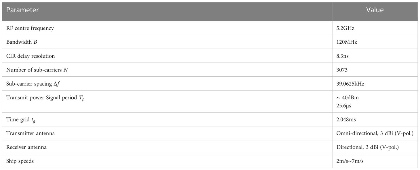
Table 1 Channel sounder settings.
During the measurement, the transmitter was located on the ship Hermann Marwede (in Figure 1) of the German Maritime Search and Rescue Service (DGzRS). The receiver was located on the ship Neuwerk (in Figure 2) of the German Federal Waterways and Shipping Administration (WSV). At the transmitter, a vertically polarized signal was periodically transmitted with a repetition rate of Tp = 25.6 µs, such that a maximum detour of 7.6 km smaller than the distance between the transmitter and the receiver can be measured. At the receiver, an omnidirectional single antenna was applied. Both ships moved at a speed of between 2 and 7 m/s most of the time. Geodetic GNSS receivers were used at the transmitter and receiver to obtain the antenna positions. The GNSS receivers are capable of receiving satellite signals from the GPS, the GLONASS, and the Galileo system. The measured data were later post-processed with real-time kinematic data to improve the positioning accuracy to the sub-meter level. To achieve synchronization between the transmitter and the receiver, two Rubidium clocks were used, one on each side. At the beginning of every measurement day, a reference measurement, where the transmit antenna had a clear line of sight (LoS) to the receive antenna, was performed to measure the time offset between transmitter and receiver clocks. To compensate for the relative clock drift between transmitter and receiver clocks, the GNSS receivers’ clocks driven by Rubidium clocks were compared to the GPS time. Therefore, the relative clock drift between the transmitter and receiver clocks can be obtained by the GPS time information. A more detailed description of clock monitoring using GPS measurements can be found in Schneckenburger et al. (2013).
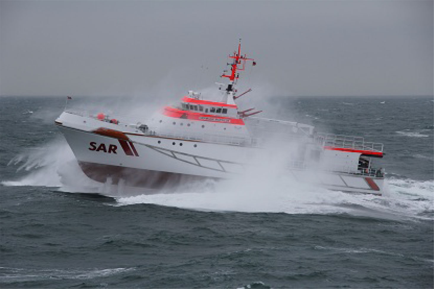
Figure 1 Photo of the Hermann Marwede in rough waters with the transmitter antenna mounted on the mast, sailing in parallel to the Neuwerk while passing her.
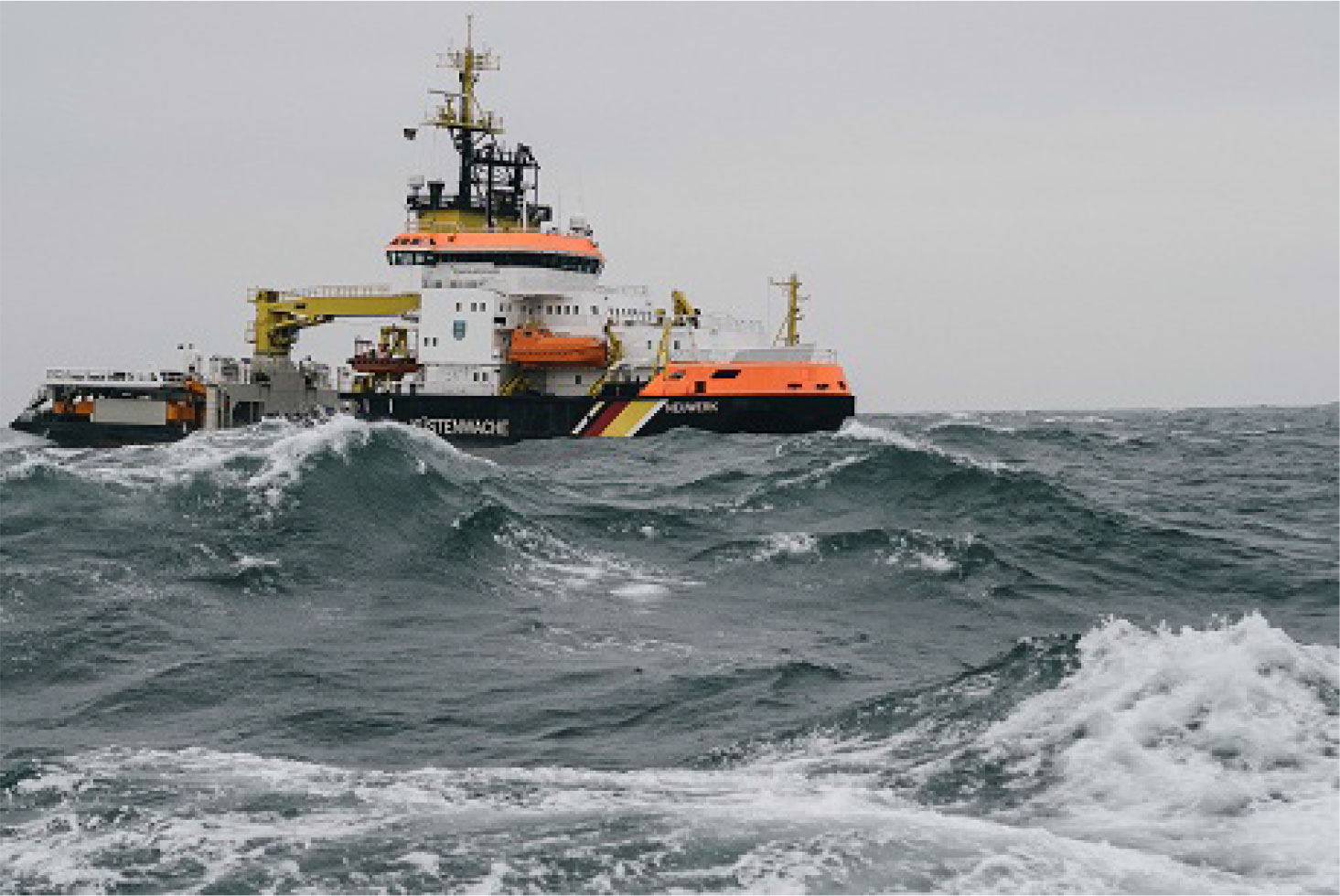
Figure 2 Photo of the Neuwerk in rough waters with the receiver antennas mounted on the topmast, sailing next to the Hermann Marwede.
During the measurement (January 27–30, 2016), the significant wave height hs of the ocean waves was approximately 2.5 m (Borgert, 2016), where significant wave height is defined as the top 33% of the largest waves. The salinity of the seawater was approximately 3.4%, and the water temperature was approximately 6°C. Detailed environmental data within the measurement time period were provided by the database of the Federal Maritime and Hydrographic Agency of Germany (BSH) (und Schifffahrtsverwaltung des Bundes (WSV), 2016). An AIS receiver was also used to record the positions of other vessels in the vicinity of Heligoland during the measurement period.
Both ships circled the island of Heligoland and the dune island. Figure 3 shows the height profile of the island and the dune. The island of Heligoland on the western side is built of substantial rocks with a height of up to 60 m compared to the dune on the eastern side with a height of less than 5 m. The vessels used different tracks around the islands and crossed in between both islands before the tide stopped further passing. Two scenarios were executed for the campaign: in the first scenario, both ships were moving in the anti-parallel way as shown in Figure 3. In the second scenario, both ships were positioned behind each other. Then, the ship Hermann Marwede gave chase, sailing in parallel and finally overtaking the ship Neuwerk. The scenario was pursued west of Heligoland island with enough space between the ships. The rocky part of the island could also act as a reflector. The sea conditions were quite rough with wave heights in the range of up to 3 m (Borgert, 2016).
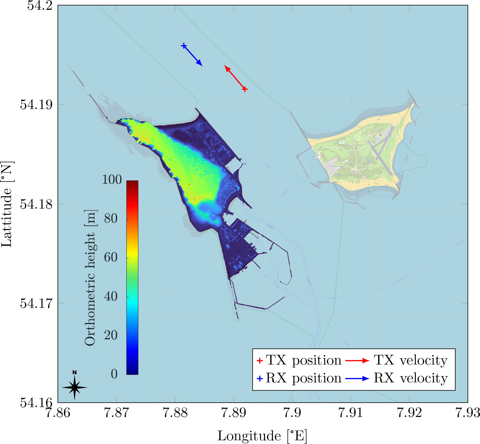
Figure 3 Positions of transmitter (TX) and receiver (RX) north of the Heligoland main island for the measurement scenario introduced in this paper. The TX is located at PTX = (N54.191 542°, E7.891 928°) with speed υTX = 5.7 m/s and Course Over Ground (COG) 320°. The RX is located at PRX = (N54.195 920°, E7.881 509°) with speed υRX = 5.4 m/s and COG 138°. The orthographic height (height above mean sea level) of the Heligoland main island terrain is shown as a color plot.
In this section, we introduce the channel propagation model for a ship-to-ship radio link. We separate the common channel propagation aspects over land and sea, and then, we differentiate between both areas where needed. Both models are distinguished by the contributions of the scatterer. On land, larger and distant components are crucial and modeled by larger planes. On sea, smaller and dynamic components are more meaningful to account for rougher sea conditions, and therefore, the planes are split up into much smaller tiles.
In this section, we present a general model applicable to sea and land propagation that considers the following:
● LoS component,
● coherent or specular reflection component from a tile of the flat sea surface, and
● incoherent or scattering components from multiple tiles caused by the rough sea surface
using the physical optical (PO) model. The effective size of the flat sea surface that is responsible for the specular reflection depends on the roughness of the sea. It is theoretically infinite for a flat sea surface and tends to zero as the sea surface becomes rougher. In order to simplify the geometry and to reduce the computational complexity of the incoherent component, a flat earth is assumed in this paper. Figure 4 shows the general setting between a transmitter and a receiver with the geometric constellation of the individual components when the sea surface plane is divided into several tiles with a dimension of 1 m × 1 m.
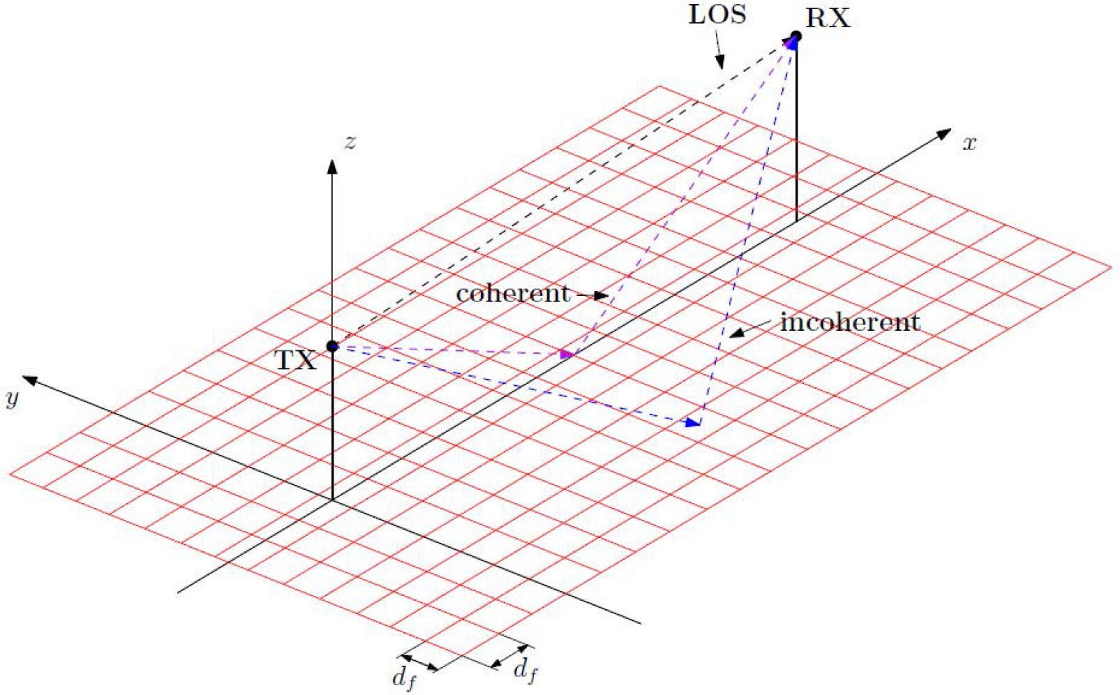
Figure 4 Geometry of the computation of multipath components using the physical optical (PO) method. The sea surface area between transmitter (TX) and receiver (RX) is constructed by multiple tiles with a size of 1 m × 1 m. The tiles shall approximate realistically the sea surface. The propagation components are divided into three: 1) LoS, 2) coherent or specular, and 3) incoherent component.
Since the scattering coefficient σ0,n is angle-dependent, the values of each coefficient σ0,n for each tile on the grid are different. Therefore, the incoherent power at the receiver corresponds to the scattering contributions from the nth tile, which can be written as
where At is the tile dimensions and n denotes the tile index, and inc represents the incoherent component. Gt,inc and Gr,inc are the gains of the transmit and receive antennas, respectively, assuming a homogeneous gain G independent of the state of the ship in the water. σ0,n represents the scattering coefficient that corresponds to the nth tile and is calculated as
where β0 is the root mean square surface slope, u is the roughness parameter, and γ can be calculated as introduced in Karasawa and Shiokawa (1984). See the Appendix for more details. The received power of the LoS and coherent component is calculated by
where dLoS is the distance between the transmitter and receiver. dT,coh and dR,coh are the distances from the specular reflection point to TX and RX, respectively. Due to the fact that the equations above represent received powers without phase information we will pass to the electric field representation for each component, which enables us to coherently add up the field components to get a resulting field at the receiver. The electric fields of the LoS, and the coherent and incoherent components at the receiver can be written as
where a uniformly distributed random phase shift ϕR is added to the incoherent component. η is the wave impedance, which is η ≈ 376.7 Ω in vacuum and air. As a result, the total received electric field E within a narrow band system is given by
Further, the total received power
can be calculated straightforwardly. For wideband channel simulation, the propagation delay of paths caused by individual tiles can be incorporated within the time-variant CIR h(t,τ) as
where δ(·) is the Delta function, αLoS(t) and αcoh(t) are the amplitude of the electric field strength of the LoS component and coherent component, respectively. αn,inc(t) represents the amplitude of the impulse response of the nth tile, which is proportional to the root of the received power.
In this section, we want to present the derived maritime channel model and verify it with measurement data from the North Sea. Since the maritime scenario is non-stationary and the main influence comes from the environment around the ships, a geometric stochastic channel model is the appropriate choice for the maritime propagation model.
We consider the three types of channel components proposed by Bello (1973): the LoS component, the specular reflection component, and the scattering component. In addition, we distinguish in our model between two types of scattering: sea and land scattering. This way, we can use a different approach to model each type of scattering by exploiting its different characteristics. Sea scattering is caused by sea waves and is always present in a maritime channel. The land scattering, caused by the land and constructions, is only present when the ships are close to the land. The CIR can then be described as
The basis of the channel model is a realistic representation of the environment. Thus, we model both the sea and the land surfaces that contribute to the scattering or reflection of the radio signals. The land surfaces are modeled by a number of finite planes; see Walter et al. (2020) and Bellido-Manganell and Walter (2022) for more details. Since the ships were in the middle of the German Bight, Heligoland was the only land surface from which we received scattering and reflections. A precise description of the land scattering is obtained by modeling the cliffs and rocks of the island in a mathematical concise way described in the subsequent subsection.
Reflection points on the open sea are from the sea surface or other vessels. The sea surface reflection depends on the roughness of the sea state. A flat sea causes a nearly perfect reflection and results in deterministic two-ray propagation. If the sea state is rougher, a significant portion of the reflected signal energy is scattered in various directions and is not received (Wang et al., 2015). Figure 5 displays the three different components: 1) LoS, 2) specular from the flat sea surface, and 3) scattering from rough sea conditions. Therefore, the superposed sea-surface reflected or specular path is significantly weakened, and the LoS component dominates. The measurements described by Wang et al. (2015) were compared to the propagation model ITU-R P.1546 (Union, 2019). For larger distances, the gap between the measurement data and the different models increases due to the increasing influence of the quantization noise of the measurement device.
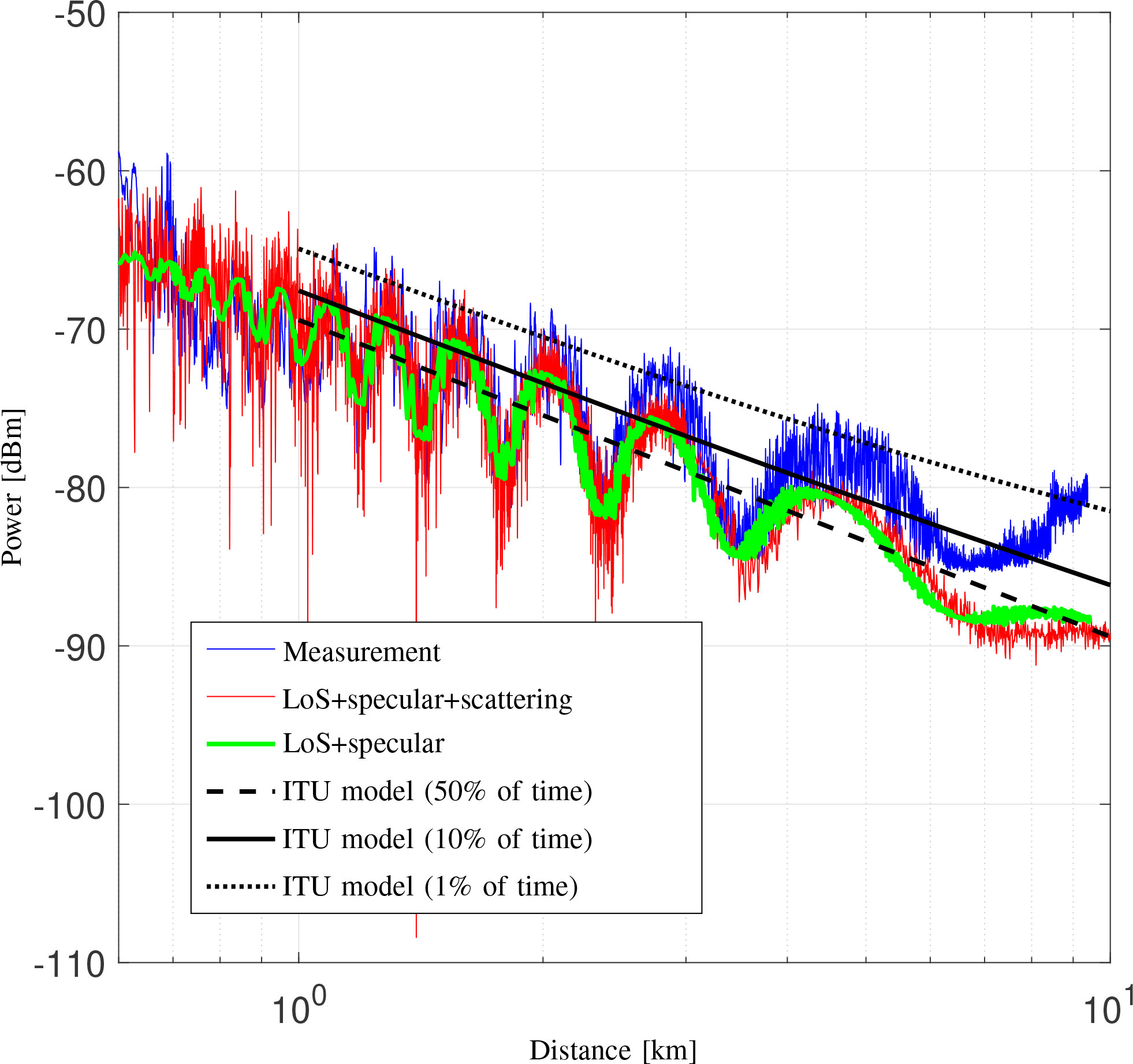
Figure 5 The measured received power level compared with the simulated power with ITU models and scattering model. The percentages of time represent that the power levels exceed 50%, 10%, and 1% of the time.
The land scattering is modeled using the channel modeling approach proposed in Bellido-Manganell and Walter (2022), which provides an analytical way of computing the delay-dependent and joint delay Doppler probability density functions (pdfs) of any mobile-to-mobile channel, and enables estimation of its quadratic delay Doppler-spread function. The environment around the ships is modeled by using infinite and finite planes where the scatterers and reflectors are assumed to be located. The approach has been validated by using channel measurement data from different dynamic campaigns addressing different aircraft-to-aircraft, drone-to-drone, vehicle-to-vehicle, and S2S scenarios. In fact, the Heligoland archipelago, which is also considered in this work, was modeled using finite and infinite planes to recreate the S2S scenario. We use the same model of the Heligoland archipelago shown in Figure 6, which consists of a total of 16 finite planes: 13 planes to model the mountain of the main Heligoland island and three planes to model the elevated buildings and constructions of both islands. The flat fields were not modeled because their contributions were negligible compared to the reflections from the prominent objects on land. This was verified by the analysis of the measured data.
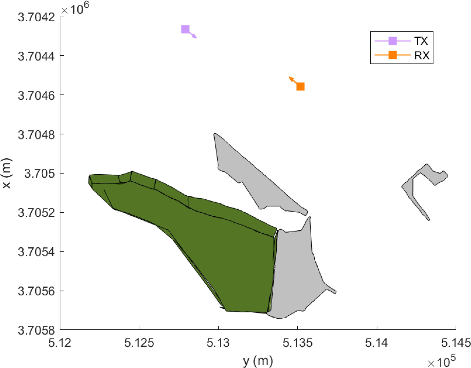
Figure 6 The model used to recreate the Heligoland archipelago and to estimate the land scattering. The mountain of the main Heligoland island is modeled using 13 finite planes (green), whereas the elevated buildings and constructions of both islands are simply modeled with three finite planes (gray). The TX (transmitter) and RX (receiver) represent the ships in the sea.
In the following, we discuss how land scattering components were derived by following the approach proposed by Bellido-Manganell and Walter (2022). First, the N planes recreating the environment were defined using a local Cartesian coordinate system. For example, the planes shown in Figure 6 were initially defined in the earth-centered, earth-fixed coordinate system using topographical data as a reference. Second, these planes were converted into a more convenient coordinate system, enabling the computation of the instantaneous delay-dependent and joint delay Doppler pdfs of the wireless channel, which were obtained following the algorithm given by Bellido-Manganell and Walter (2022, Algorithm 1)). Third, by considering that the joint delay Doppler pdf p of a channel is proportional to its delay Doppler power spectral density, as shown in Walter et al. (2017), one can use a proportionality factor Γ based on the reflection properties of the scatterers in Heligoland. In this work, we estimated the proportionality factor by comparing the pdf with the received delay Doppler power spectral density.
In the channel measurements, however, the LoS component is not shown as ideally expected as a discrete point in the delay Doppler domain. However, it is depicted as two multiplying sinc functions centered at τLoS and fd,LoS and spanning both delay and Doppler directions. As shown in Bellido-Manganell and Walter (2022, Appendix 1), this is caused by the time- and bandwidth-limited sampling of the channel and can be recreated easily using Bellido-Manganell and Walter (2022, Equation (18)).
We now compare the channel measured during the S2S measurement campaign with the channel recreated by our channel model. For this, we use the scenario depicted in Figure 6. First, we show in Figure 7 the measured spreading function SF of the channel. The spreading function is computed using 1,024 CIRs successively measured, corresponding to an observation window of 2.0972 s. Applying our channel model to the same scenario, we obtain the channel shown in Figure 8. Although our channel model is capable of taking snapshots of the channel at specific times, for this comparison, we take multiple snapshots of the channel within the 2.0972-s observation window and average the result. Comparing Figure 7 with Figure 8, one can see that our model can reproduce the channel with good accuracy, as its dominant components are well described by our channel model. For a better understanding of how our model reproduces the channel, we also depict separately the different components considered by our channel model: the LoS component in Figure 9, the coherent sea reflection in Figure 10, the sea scattering in Figure 11, and the land scattering in Figure 12. The complete channel shown in Figure 8 consists of these components. One can see that the LoS component is well recreated by our approach and that it is significantly stronger than the other components of the channel. The specular reflection component and the sea scattering are not easily distinguishable from each other, as they both present a very similar delay and Doppler frequency shift. The land scattering is well separated from the other channel components as it arrives from a later delay and is spread over a wider Doppler range. The specular component can be checked by the mean value of the local power, and the scattered power can be checked by the variation of the power.
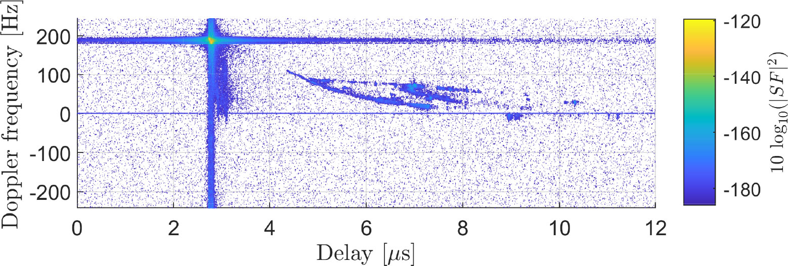
Figure 7 The measured propagation channel with the ships located at the coordinates shown in Figure 6.
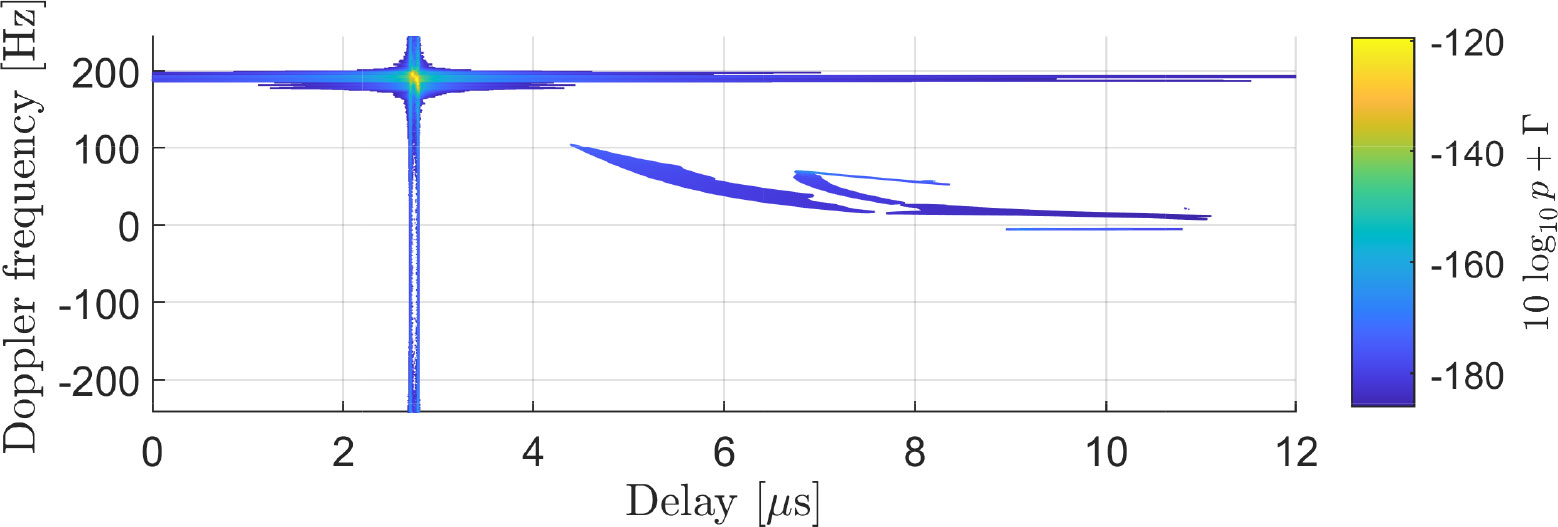
Figure 8 Recreated channel for the scenario depicted in Figure 6. We see a good match with the measured channel in Figure 7, which has richer smaller detail contributions but similar dominant components. The recreated channel here is composed of the LoS, coherent sea reflection, sea scattering, and land scattering components.
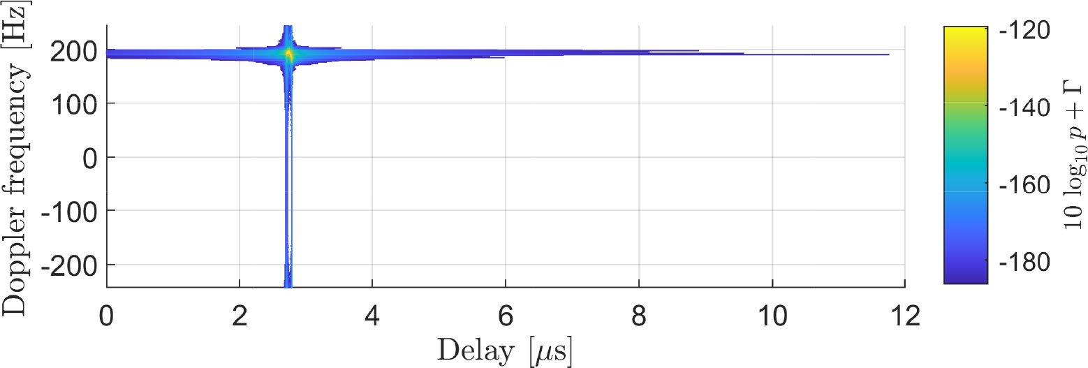
Figure 9 Modeled line-of-sight (LoS) component.
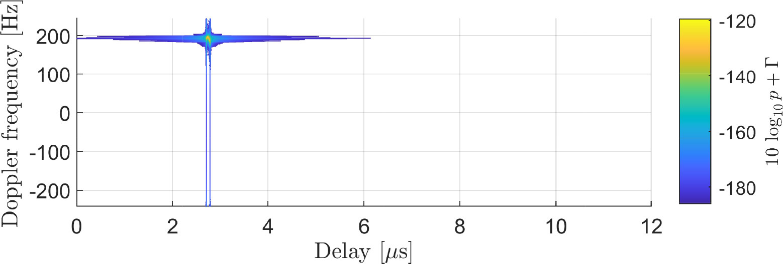
Figure 10 Coherent sea reflection component.
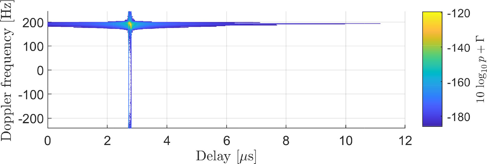
Figure 11 Sea scattering component.
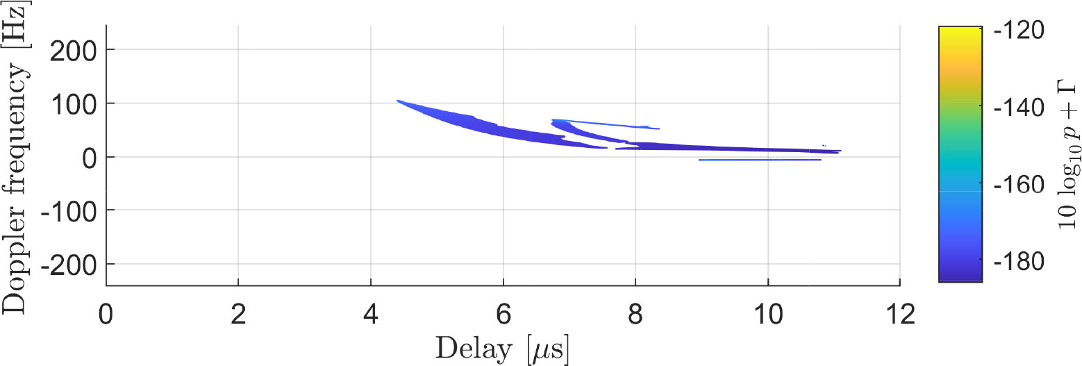
Figure 12 Land scattering component.
Wireless signal propagation in a maritime environment is significantly influenced by several factors. Apart from the direct propagation (i.e., LoS path) between the transmitter and receiver, there are several types of multipath components occurring due to reflection (referred to as specular component) and diffuse scattering (referred to as incoherent component) from the rough sea surface. Figure 13 is a plot of the three individual components, such as LoS, coherent sea surface reflection, and sea surface scattering, in terms of their contribution in power and delay.
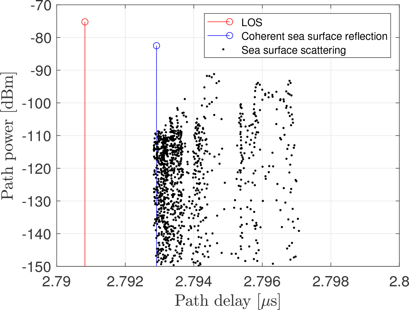
Figure 13 Model of the channel impulse response split into the individual contributions of the line of sight (LoS), the coherent sea surface reflection, and the sea scattering component. Note that a real system with limited bandwidth would not be able to resolve the individual components.
For the calculation of the incoherent sea surface scattering multipath components, we require an exemplary sea surface. For modeling such a sea surface, we build on an approach introduced by Hauser et al. (2001), where the authors define a random two-dimensional slope spectrum in the spatial frequency domain and obtain the corresponding surface slope by a two-dimensional inverse Fourier transform. In contrast to Hauser et al. (2001), we require realizations of the sea surface itself, rather than the surface slope, and continuous evolution of these realizations in time.
We generate a random realization of the sea surface in the two-dimensional spatial frequency domain as
where νx and νy are the spatial wave frequencies in the x- and y-directions. Φ(νx, νy) ∼ U(0, 2π) denotes a random process providing phase values, which are uniformly distributed in the interval [0, 2π). We achieve time dependency through another random process
which maps a temporal Gaussian distributed frequency to spatial frequencies (νx, νy). Both processes Φ(νx, νy) and f(νx, νy) are white with respect to νx and νy.
Similar to Hauser et al. (2001), we choose a non-directional spatial energy density spectrum
with , which is a Gaussian-shaped ring in the spatial frequency domain with standard deviation σp its peak at νp, both in physical unit m−1. The energy of the sea surface is calculated as
where Ẽ in Equation 14 is a lower bound, which is tight for νp ≫ σp > 0. In this case, we set Ẽ = E with a good approximation. By sampling the spatial spectrum with the sampling intervals Δνx and Δνy around the spatial frequencies zero, i.e.,
applying a two-dimensional (Nx, Ny)-point inverse discrete Fourier transform (IDFT) and taking the real part, we obtain a sampled realization of the sea surface as
The sampling intervals Δx and Δy in the spatial domain relate to the sampling intervals Δνx and Δνy, respectively, in the spatial frequency domain according to
With
we get an approximation of the root mean square sea surface height
Note that we obtain a real-valued sea surface realization in Equation 17 by taking the real part of the IDFT of the corresponding complex-valued realization Su,v(t) in the spatial frequency domain. Consequently, due to statistics, we can only conclude that approximately half of the energy goes into the real part, which, in Equation 19, requires the approximation (“≈”) and a factor of 2 to compensate for halving the energy.
Figures 14, 15 show the spatial energy density spectrum according to Equation 14 and a corresponding sea surface realization according to Equation 17 for νp = 5 × 10⁻³ m−1, σp = 10−3 m−1, Hrms = 4 m, Δx = Δy = 1 m, and Nx = Ny = 4000. The mean νT and standard deviation σT of the Gaussian random process for drawing the frequencies f(νx, νy) in Equation 13 are not relevant for plotting a single snapshot in time. For our simulations, we choose νT = 0.1 Hz and σT = 7 × 10⁻³ Hz, which is inferred from sea surface observations in the measurement area around Heligoland on January 27, 2016.
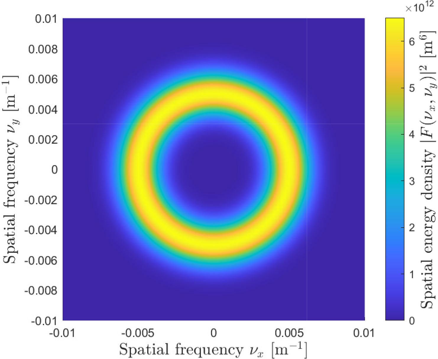
Figure 14 Sea surface spatial energy density spectrum according to Equation 14 and a corresponding sea surface realization for , σp = 10−3 m−1, Hrms = 4m, Δx = Δy = 1m and Nx = Ny = 4000.
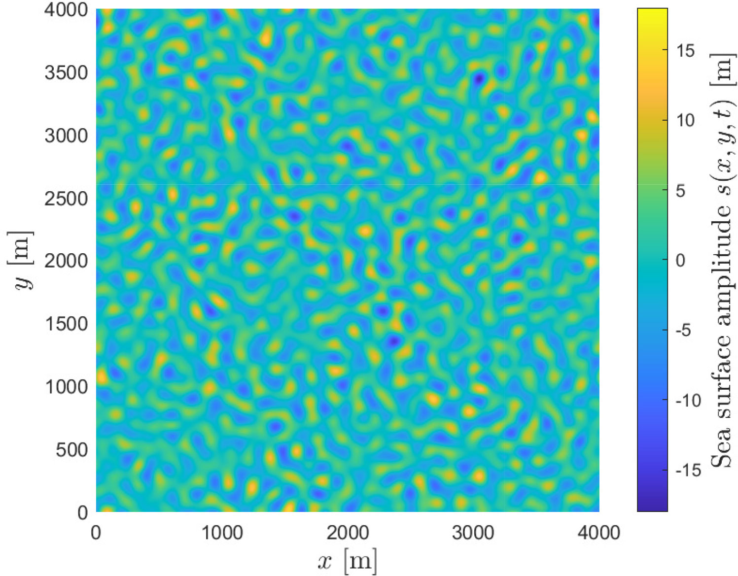
Figure 15 Two-dimensional sea surface realization according to equation 17 of Figure14.
Figure 4 illustrates the basic assumption of geometry for the PO model to compute the coherent or specular and incoherent components caused by the sea surface. The mean sea surface lies in the xy-plane and is divided into individual tiles with dimensions , as indicated by the red grid. TX and RX are located at (0, 0, hTX)T and (d, 0, hRX)T, respectively, where hTX and hRX are the antenna heights above mean sea level (MSL) and d is the horizontal distance between TX and RX. The dashed lines represent three different components, where black is the LoS component, purple is the coherent or specular component, and blue is the incoherent component. Due to the significant value of the fundamental wave where small and intense variations of the ocean surface occur, we further extend the geometric model from Figures 4, 16 with an exemplary sea surface. Since each tile has a different orientation, the normal vectors are calculated for all tiles. Using these normal vectors, we assume a local Cartesian coordinate system for each tile. In this way, the local incidence, scattering, and azimuth angles with respect to the TX and RX positions are computed for each tile. Consequently, the coherent component and incoherent components caused by each tile on the sea surface are calculated according to the descriptions in Section 4.1.

Figure 16 Random sea surface considering the fundamental waves. The actual height is shown by the color bar and the parameter set of the corresponding sea surface realization for , Hrms = 1 m, Δx = Δy = 1 m, and Nx = Ny = 200.
Other practical parameters that are considered by the channel propagation model are the antenna heights, on either the transmitter or the receiver, above sea level. The antenna heights define the reflection points on the sea and land. The antenna height parameter has been verified by Wang et al. (2015). Maritime broadband wireless communication systems currently use bandwidths of up to 20 MHz. The measured data were also examined to assess the correlation within the 100-MHz bandwidth between different sub-bands. We also validated the model by using the measurement data used in our simulation code (Wang et al., 2019).
This paper summarizes the radio link channel propagation between two moving ships at sea, considering dynamic sea conditions as well as nearby coastal areas. The channel model is presented as a geometric stochastic channel model with a flexible and generic parameter set. The parameters have been derived and validated using measurement data collected with a channel sounder. The analysis is based on measurement data in the C-Band of 5.2 GHz, which is of great interest since the band below 6 GHz is crucial for maritime broadband communications. Further, it could also be used for ranging and thus be applicable for alternative navigation applications. All this is considered by the channel model simulation code, which is available on Code Ocean.
The raw data supporting the conclusions of this article will be made available by the authors, without undue reservation.
RR conceived and directed the presented project. MW and MB-M developed the modeling of the land-sided component. WW and AD developed the modeling of the sea effects. AD and MB-M provided the Matlab code for publication. All authors contributed to the writing of the manuscript. All authors contributed to the article and approved the submitted version.
We thank the Wasserstraßen- und Schifffahrtsverwaltung des Bundes (WSV) for providing the data about water heights provided by the Bundesanstalt fuer Gewaesserkunde (BfG). We thank the crews of the WSV Neuwerk and the Hermann Marwede from the Deutsche Gesellschaft zur Rettung Schiffbruechiger (DGzRS). We thank the Institute of Optical Sensor Systems at DLR Berlin for providing the DEM data of Heligoland.
The authors declare that the research was conducted in the absence of any commercial or financial relationships that could be construed as a potential conflict of interest.
All claims expressed in this article are solely those of the authors and do not necessarily represent those of their affiliated organizations, or those of the publisher, the editors and the reviewers. Any product that may be evaluated in this article, or claim that may be made by its manufacturer, is not guaranteed or endorsed by the publisher.
3rd Generation Partnership Project (3GPP). (2022). Technical Specification Group Services and System Aspects; Maritime Communication Services over 3GPP system; Stage 1 (Release 17). (Tech. rep., 3GPP).
3rd Generation Partnership Project (3GPP). (2023). Technical Specification Group Services and System Aspects; Service requirements for cyberphysical control applications in vertical domains; Stage 1 (Release 19) (Tech. rep., 3GPP).
Allianz (2022). Safety and shipping review 2022 - an annual review of trends and developments in shipping losses and safety. Allianz Commercial’s annual Safety and Shipping Review. 1–66. Available at: https://commercial.allianz.com/news-and-insights/reports/shipping-safety.html.
Alqurashi F. S., Trichili A., Saeed N., Ooi B. S., Alouini M.-S. (2022). Maritime communications: A survey on enabling technologies, opportunities, and challenges. IEEE Internet Things J. 10 (4), 1–1. doi: 10.1109/JIOT.2022.3219674
Beckmann P., Spizzichino A. (1987). The Scattering of Electromagnetic Wave from Random Rough Surfaces (Artech House).
Bellido-Manganell M. A., Walter M. (2022). Non-stationary 3d m2m channel modeling and verification with aircraft-to-aircraft, drone-to-drone, vehicle-to-vehicle, and ship-to-ship measurements (IEEE Transactions on Vehicular Technology).
Bello P. (1973). Aeronautical channel characterization. IEEE Trans. Commun. 21, 548–563. doi: 10.1109/TCOM.1973.1091707
Borgert H. (2016). Beobachtete Wellendaten in der Nordsee vom 26.1.2016 bis 31.1.2016 (Tech. rep., Oceanwaves).
Du J., Song J., Ren Y., Wang J. (2021). Convergence of broadband and broadcast/multicast in maritime information networks. Tsinghua Sci. Technol. 26, 592–607. doi: 10.26599/TST.2021.9010002
Forti N., d’Afflisio E., Braca P., Millefiori L. M., Carniel S., Willett P. (2022). Next-Gen intelligent situational awareness systems for maritime surveillance and autonomous navigation. Proc. IEEE 110, 1532–1537. doi: 10.1109/JPROC.2022.3194445
Guan S., Wang J., Jiang C., Duan R., Ren Y., Quek T. Q. S. (2021). Magicnet: The maritime giant cellular network. IEEE Commun. Magazine 59, 117–123. doi: 10.1109/MCOM.001.2000831
Hauser D., Soussi E., Thouvenot E., Rey L. (2001). SWIMSAT: A real-aperture radar to measure directional spectra of ocean waves from space — main characteristics and performance simulation. J. Atmospheric Oceanic Technol. 18, 421–437. doi: 10.1175/1520-0426(2001)018<0421:SARART>2.0.CO;2
Jo S., Shim W. (2019). LTE-maritime: High-speed maritime wireless communication based on LTE technology. IEEE Access 7, 53172–53181. doi: 10.1109/ACCESS.2019.2912392
Karasawa Y., Shiokawa T. (1984). Characteristics of L-band multipath fading due to sea surface reflection. IEEE Trans. Antennas Propag 32, 618–623. doi: 10.1109/TAP.1984.1143365
Mathworks. (2021). MATLAB version 9.10.0.1613233 (R2021a). (Natick, Massachusetts: The Mathworks, Inc.).
Mehrnia N., Ozdemir M. K. (2016). “Novel maritime channel models for millimeter radiowaves,” in 2016 24th International Conference on Software, Telecommunications and Computer Networks (SoftCOM), Split, Croatia, 1–6. doi: 10.1109/SOFTCOM.2016.7772162
Paolo F., Gianfranco F., Luca F., Marco M., Andrea M., Francesco M., et al. (2021). Investigating the role of the human element in maritime accidents using semi-supervised hierarchical methods. Transp. Res. Procedia 52, 252–259. doi: 10.1016/j.trpro.2021.01.029
Sadlier G., Flytkjær R., Sabri F., Herr D. (2017). The economic impact on the UK of a disruption to GNSS (London Economics: Tech. rep.).
Schneckenburger N., Elwischger B., Belabbas B., Shutin D., Circiu M., Suss M., et al. (2013). “Ldacs1 navigation performance assessment by flight trials,” in The European Navigation Conference (ENC). Vienna, Austria 1–5.
Smith B. (1967). Geometrical shadowing of a random rough surface. IEEE Trans. Antennas Propag 15, 668–671. doi: 10.1109/TAP.1967.1138991
Soatti G., Nicoli M., Garcia N., Denis B., Raulefs R., Wymeersch H. (2018). Implicit cooperative positioning in vehicular networks. IEEE Trans. Intelligent Transportation Syst. 19, 3980–3964. doi: 10.1109/TITS.2018.2794405
Tao W., Zhu M., Chen S., Cheng X., Wen Y., Zhang W., et al. (2022). Coordination and optimization control framework for vessels platooning in inland waterborne transportation system. IEEE Trans. Intelligent Transportation Syst., 1–20. doi: 10.1109/TITS.2022.3220000
Thombre S., Zhao Z., Ramm-Schmidt H., Vallet Garcıa J. M., Malkamaki T., Nikolskiy S., et al. (2022). Sensors and ai techniques for situational awareness in autonomous ships: A review. IEEE Trans. Intelligent Transportation Syst. 23, 64–83. doi: 10.1109/TITS.2020.3023957
und Schifffahrtsverwaltung des Bundes (WSV), W. (2016). Pegelstaende. Tech. rep., Wasserstraßen- und Schifffahrtsverwaltung des Bundes (WSV), bereitgestellt durch die Bundesanstalt fuer Gewaesserkunde (BfG).
Union I. T. (2019). Recommendation ITU-R P.1546: Method for point-to-area predictions for terrestrial services in the frequency range 30 MHz to 4 000 MHz. (Tech. rep., ITU).
Walter M., Shutin D., Dammann A. (2017). Time-variant Doppler PDFs and characteristic functions for the vehicle-to-vehicle channel. IEEE Trans. Veh Technol. 66, 10748–10763. doi: 10.1109/TVT.2017.2722229
Walter M., Shutin D., Schmidhammer M., Matolak D. W., Zajic A. (2020). Geometric analysis of the Doppler frequency for general non-stationary 3D mobile-to-mobile channels based on prolate spheroidal coordinates. IEEE Trans. Vehicular Technol. 69, 10419–10434. doi: 10.1109/TVT.2020.3011408
Wang W., Hoerack G., Jost T., Raulefs R., Walter M., Fiebig U. (2015). “Propagation channel at 5.2 GHz in Baltic sea with focus on scattering phenomena,” in 2015 9th European Conference on Antennas and Propagation (EuCAP). Lisbon, Portugal 1–5. Available at: https://ieeexplore.ieee.org/abstract/document/7228342.
Wang W., Raulefs R., Jost T. (2019). Fading characteristics of maritime propagation channel for beyond geometrical horizon communications in c-band. CEAS Space J. 11, 95–104. doi: 10.1007/s12567-017-0185-1
Wang J., Zhou H., Li Y., Sun Q., Wu Y., Jin S., et al. (2018). Wireless channel models for maritime communications. IEEE Access 6, 68070–68088. doi: 10.1109/ACCESS.2018.2879902
Yang K., Molisch A. F., Ekman T., Røste T., Berbineau M. (2019). A round earth loss model and small-scale channel properties for open-sea radio propagation. IEEE Trans. Vehicular Technol. 68, 8449–8460. doi: 10.1109/TVT.2019.2929914
S is the shadowing factor Smith (1967). Γrough is the Fresnel reflection coefficient for a rough sea surface and specified polarization. Under the assumption of a random Gaussian distributed height variation of the water surface, the reflection coefficient of the rough surface Γrough is given as (Beckmann and Spizzichino, 1987) , with the wavelength λ, the RMS of the water wave height h0, incident angle β, a shadowing factor S provided by Smith (1967), and the reflection coefficient Γ of the smooth surface given in Molisch (2010).
In this section, we sketch the concept of the maritime components of sea surface scattering that are responsible for the dynamically changing environment. The land-based components are part of the simulation code that is described in Bellido-Manganell and Walter (2022).
Figure 17 shows the class diagram of the unified modeling language based on three classes representing the sea surface scattering with additional two classes, which represent the motion of the ship. The channel model representing sea surface scattering is implemented by three Matlab classes, which are
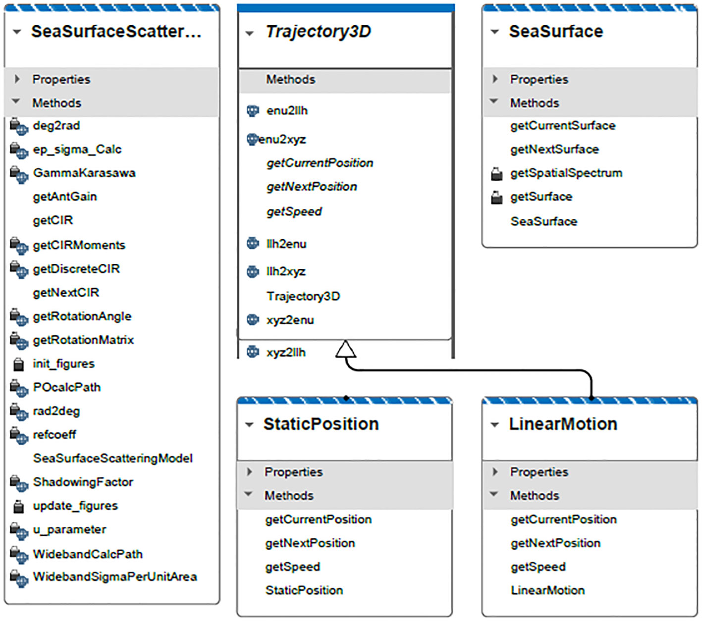
Figure 17 Matlab sea surface scattering channel model classes.
● SeaSurfaceScatteringModel,
● SeaSurface, and
● Trajectory3D.
The SeaSurfaceScatteringModel is the main class for calculating and providing the channel impulse response. The channel impulse response calculation is based on the current sea surface realization, provided by an object of class SeaSurface, and the current position of TX and RX, provided by one object of a subclass of Trajectory3D each. The signature of the class’ constructor SeaSurfaceScatteringModel consists of the following arguments:
● SeaSurfaceScatteringModel,
● SeaSurface, and
● Trajectory3D.
The relevant methods for the operation of this class are
● SeaSurfaceScatteringModel,
● SeaSurface, and
● Trajectory3D.
Class SeaSurface provides the implementation of a model, generating a dynamic sea surface realization. The principle of the implementation is shown in Hauser et al. (2001, Sec. 3.b.). An abstract class provides the definition of methods to obtain the three-dimensional trajectories of TX and RX. Subclasses inherit from this abstract class and provide the implementation of the method, defined in the abstract class Trajectory3D. The class StaticPosition provides the current position and indicates it is a static position. The class LinearMotion provides the current position, the velocity, and a linear motion model of the ship. The simulation code of the channel model will be published on Code Ocean.
Keywords: channel model, maritime communication, maritime navigation, broadband, over-sea communications
Citation: Raulefs R, Bellido-Manganell MA, Dammann A, Walter M and Wang W (2023) Verification and Modeling of the Maritime Channel for Maritime Communications and Navigation Networks. Front. Mar. Sci. 10:1158524. doi: 10.3389/fmars.2023.1158524
Received: 04 February 2023; Accepted: 18 July 2023;
Published: 06 November 2023.
Edited by:
Kun Yang, Zhejiang Ocean University, ChinaReviewed by:
Hongming Zhang, Beijing University of Posts and Telecommunications (BUPT), ChinaCopyright © 2023 Raulefs, Bellido-Manganell, Dammann, Walter and Wang. This is an open-access article distributed under the terms of the Creative Commons Attribution License (CC BY). The use, distribution or reproduction in other forums is permitted, provided the original author(s) and the copyright owner(s) are credited and that the original publication in this journal is cited, in accordance with accepted academic practice. No use, distribution or reproduction is permitted which does not comply with these terms.
*Correspondence: Ronald Raulefs, Um9uYWxkLlJhdWxlZnNAZGxyLmRl
Disclaimer: All claims expressed in this article are solely those of the authors and do not necessarily represent those of their affiliated organizations, or those of the publisher, the editors and the reviewers. Any product that may be evaluated in this article or claim that may be made by its manufacturer is not guaranteed or endorsed by the publisher.
Research integrity at Frontiers
Learn more about the work of our research integrity team to safeguard the quality of each article we publish.