Demystifying image-based machine learning: a practical guide to automated analysis of field imagery using modern machine learning tools

Image-based machine learning methods are becoming among the most widely-used forms of data analysis across science, technology, engineering, and industry. These methods are powerful because they can rapidly and automatically extract rich contextual and spatial information from images, a process that has historically required a large amount of human labor. A wide range of recent scientific applications have demonstrated the potential of these methods to change how researchers study the ocean. However, despite their promise, machine learning tools are still under-exploited in many domains including species and environmental monitoring, biodiversity surveys, fisheries abundance and size estimation, rare event and species detection, the study of animal behavior, and citizen science. Our objective in this article is to provide an approachable, end-to-end guide to help researchers apply image-based machine learning methods effectively to their own research problems. Using a case study, we describe how to prepare data, train and deploy models, and overcome common issues that can cause models to underperform. Importantly, we discuss how to diagnose problems that can cause poor model performance on new imagery to build robust tools that can vastly accelerate data acquisition in the marine realm. Code to perform analyses is provided at https://github.com/heinsense2/AIO_CaseStudy.

1 Introduction

Imagery from the ocean has long been used to survey marine environments, quantify physical conditions, and monitor the inhabitants of marine ecosystems (Longley and Martin, 1927; Drew, 1977; Beijbom et al., 2015; Lombard et al., 2019; Marochov et al., 2021). This reliance on imagery as a means of extracting data from marine systems has only grown with the increasing accessibility of satellite imagery and the decreasing cost and increasing quality of imaging systems that can be deployed directly in the field (Durden et al., 2016; Williams et al., 2019; Bamford et al., 2020; Rodriguez-Ramirez et al., 2020). Yet visual data bring with them some unique challenges. Images and video are expensive to process due in part to the fact that imagery is inherently high-dimensional; for example, a single grayscale image of one-megapixel resolution, a coarse image by modern standards, is a 2²⁰-dimensional data object. Researchers who collect imagery in the course of their work often return from field campaigns with terabytes to petabytes of such high-dimensional imagery that must then be processed (Schoening et al., 2018).

The role of image analysis (see Table 1 for glossary of bolded terms) is to compress high-dimensional visual data into much lower-dimensional summaries relevant to a particular task or study objective. As humans, we perform this type of visual data compression naturally (Marr, 1982). We look at an image and with proper training, can classify what is present in the image, localize and count distinct objects, and partition the image into regions of one type or another. The objective of image-based machine learning (ML), a subfield of computer vision, is to train computer algorithms to perform these same tasks with a high level of accuracy. Doing so can tremendously accelerate image processing and greatly reduce its cost (Norouzzadeh et al., 2018), while also providing an explicit, standardized, and reproducible workflow that can be shared easily among researchers and applied to new problems (Goodwin et al., 2021; Katija et al., 2022). Despite the promise of these methods, the expertise required to apply, adapt, and troubleshoot ML methods using the kinds of image datasets marine scientists collect still creates a high barrier to entry (Crosby et al., 2023).

TABLE 1

Table 1 Glossary of terms relevant to image-based machine learning.

A number of recent articles provide overviews of how modern image-based machine learning methods work and how these methods have been applied to problems in marine science (e.g., Michaels et al., 2019; Goodwin et al., 2021; Li et al., 2022). Here, we focus on the practical problem of how to implement image-based ML pipelines on real imagery from the field. The remainder of this paper is structured as a sequence of steps involved in defining an analytical task to be solved, preparing training data, training and evaluating models, deploying models on new data, and diagnosing and fixing performance issues. To provide concreteness, we present a running case study: object detection of marine species using imagery and software tools from the open source FathomNet database and interface (Katija et al., 2022). We use this case study to demonstrate each phase of constructing and troubleshooting a ML pipeline, and we provide code and guidelines needed to reproduce each step in a github repository: https://github.com/heinsense2/AIO_CaseStudy.

1.1 Building and using a machine learning pipeline

Researchers often have a clear idea of how they want to use the data extracted from imagery. This idea forms the starting point for designing a machine learning pipeline to automatically extract data from imagery. Building a machine learning pipeline to solve image analysis tasks involves a series of steps:

1.1.1 Define an analytical task

This step requires working to define the objective of image analysis and the target metrics to be extracted from imagery. The type of imagery to be analyzed should be specified. This step may also involve defining performance criteria and setting benchmarks for acceptable performance.

1.1.2 Generate and organize training and testing datasets

This step involves developing and organizing image libraries for training, testing, and deploying models. This involves both organizing imagery with appropriate file structure and, very often, hand-labeling ground truth data to be used to train and test models. This step requires software tools that allow a researcher to organize images and to label, or annotate, imagery so it can be later used to train and test machine learning models.

1.1.3 Select and train appropriate machine learning models

This step requires identifying a machine learning model architecture capable of performing the desired image analysis task, as well as software and hardware implementations capable of training and deploying the model to perform inference on new imagery.

1.1.4 Evaluate model performance

This step involves summarizing and visualizing model predictions and performance measures, and often comparing these measures across alternative model architectures or training schedules.

1.1.5 Diagnose performance issues and apply interventions to improve performance

This step involves applying a trained model to new imagery and re-evaluating its performance. If performance is below target levels, it may be necessary to modify training methods, datasets, or model architecture to improve performance.

In the following sections, we walk through each of these steps to illustrate how each is accomplished, and how the steps combine to produce an adaptable pipeline with robust performance.

2 Defining an image analysis task

2.1 Overview

Defining the image analysis task to be solved is the first step in any machine learning pipeline. Is the goal to assign an image to one class or another – for example, to decide whether a particular species is or is not present or a particular environmental condition is or is not met? Or is the aim instead to identify and count objects of interest – for example, to find all crustaceans in an image and identify them to genus? Or is the objective to divide regions of the image into distinct types and quantify the prevalence of those types – for example, to partition the fraction of a benthic image occupied by different algae or coral morphotypes? The answers to these questions determine how one proceeds with gathering appropriate labeled data, selecting and training a model, and deploying that model on new data.

2.2 Technical considerations

Many of the traditional problems marine scientists currently use imagery to address fall into one of three categories: image classification, object detection, or semantic segmentation. More complex tasks such as tracking (Katija et al., 2021; Irisson et al., 2022), functional trait analysis (Orenstein et al., 2022), pose estimation (Graving et al., 2019), and automated measurements (Fernandes et al., 2020) often rely on these more basic tasks as building blocks.

In image classification problems, a computer program is presented with an image and asked to assign the image to one of a set of classes. Classes could be defined based on the presence or absence of particular objects (e.g., shark present or shark absent; Sharma et al., 2018), or represent a set of categories to which the image must be assigned, for example on the basis of what kind of animal is present in the image (Piechaud et al., 2019) or what type of habitat is represented in the image (Jackett et al., 2023). An important distinction between whole-image classification and other common image analysis tasks is that in image classification, classes are assigned at the scale of the entire image (Chapelle et al., 1999; Fei-Fei et al., 2004). Thus, objects of interest are not spatially localized within the image, nor does the model provide information on the properties of individual pixels or spatial regions within the image. Whole image classification is appropriate for some tasks, such as simply detecting the presence or absence of a particular species of interest or environmental condition, but is less appropriate for others, for example, counting individuals of a particular species when multiple individuals can occur within a single image (Beery et al., 2021). Nevertheless, this task remains relevant in many automated image analysis problems (Qin et al., 2016; Villon et al., 2021; Kyathanahally et al., 2022) and is the approach of choice for certain types of marine microscopy data where images are typically stored as extracted region of interest (e.g., Luo et al., 2018; Ellen et al., 2019).

A second common task involves detecting and spatially localizing objects of interest within images, a task known as object detection or instance segmentation. Separating instances of the same type of object (e.g., there are nine fish identified as Atlantic cod in this image) in a given image is often crucial if imagery is being used to estimate abundances (Moeller et al., 2018), and most object detection pipelines can also be trained to detect objects of many different classes, which is valuable for analyzing images that contain multiple objects of interest that belong to different classes (see Scoulding et al., 2022 for a discussion of limitations at high density).

A third task, known as semantic segmentation, involves assigning a class to each pixel in an image. Semantic segmentation differs from object detection in that one is not interested in detecting and discriminating instances of a particular class, but rather in determining the class membership of each pixel in an image. This can be useful for tasks such as estimating the percent cover of algae, corals, or other benthic substrate types (e.g., Beijbom et al., 2015; Williams et al., 2019). If images are collected in a controlled and standardized way, the percentage of each image occupied by different species or classes of object can be estimated by the relative abundance of pixels assigned to each class.

Image-based ML tools have also been used for a variety of applications beyond the three tasks described above. Examples include “structure-from-motion” studies, in which the three-dimensional structure of objects are inferred and reconstructed from a sequence of images taken from different locations in the environment (Francisco et al., 2020), animal tracking and visual field reconstruction (Hein et al., 2018; Fahimipour et al., 2023), quantitative measurement and size estimation (Fernandes et al., 2020), animal postural analysis (Graving et al., 2019), and re-identification of individual animals in new images based on a set of previous observations (Nepovinnykh et al., 2020).

2.3 Case study: species detection and classification from benthic and midwater imagery

To provide a concrete example, we consider an object detection and classification task that seeks to localize and identify marine animals in deep-sea imagery collected from the Eastern Pacific within the Monterey Bay and surrounding regions. Images were collected by the Monterey Bay Aquarium Research Institute (MBARI) during Remotely Operated Vehicle (ROV) surveys conducted between 1989 and 2021 (Robison et al., 2017), and are housed in the open-source FathomNet database (FathomNet.org; Katija et al., 2022). We focus on six common biological taxa that are observed broadly across the sampling domain, at a range of depths, and over several decades of sampling (Figure 1. shows iconic image of each class): the fish genera Sebastes (Rockfish) and Sebastolobus (Thornyheads), and the squid species Dosidicus gigas (Humboldt squid), Chiroteuthis calyx (swordtail squid), Gonatus onyx (black-eyed squid), and the siphonophore, Nanomia bijuga. Although classes of interest are sometimes clearly visible in images as shown in Figure 1, FathomNet contains many images with small subjects, complex visual backgrounds, heterogeneous lighting, and a host of other challenging visual conditions (Figure 2) that are ubiquitous in marine science applications.

FIGURE 1

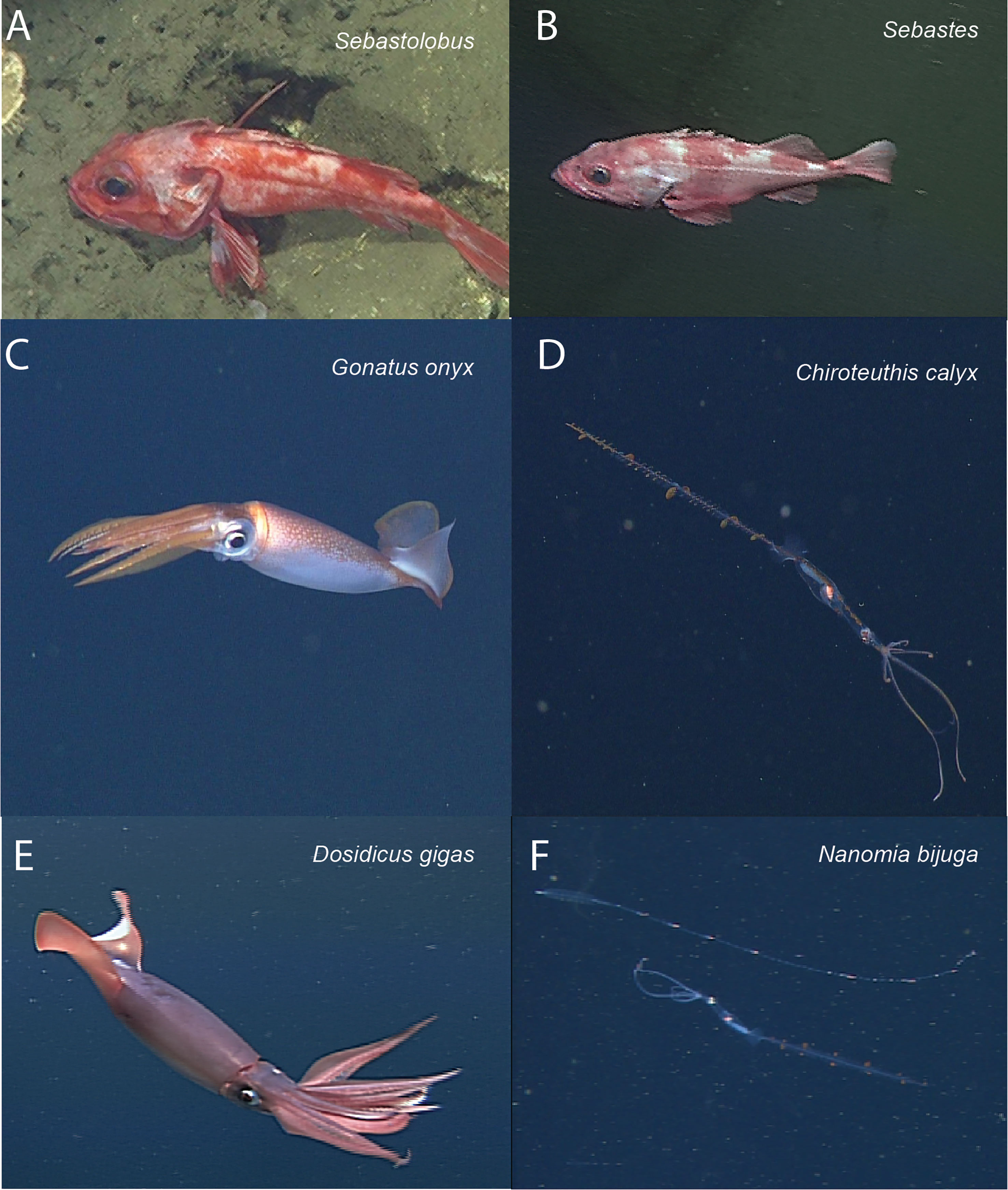
Figure 1 Focal species included in case study (iconic images). Focal species included fish in the genera Sebastolobus (A) and Sebastes (B), squid species Gonatus onyx (C) Chiroteuthis calyx (D), and Dosidicus gigas (E). Panel (F) shows an image of the siphonophore, Nanomia bijuga, alongside a juvenile C. calyx (F, lower organism in image), which are believed to visually and behaviorally mimic N. bijuga (Burford et al., 2015). Images in panels (A-F) were selected for clarity and subjects are enlarged for visualization. (Figure 2) shows focal species in images that are more representative of typical images in FathomNet.

FIGURE 2

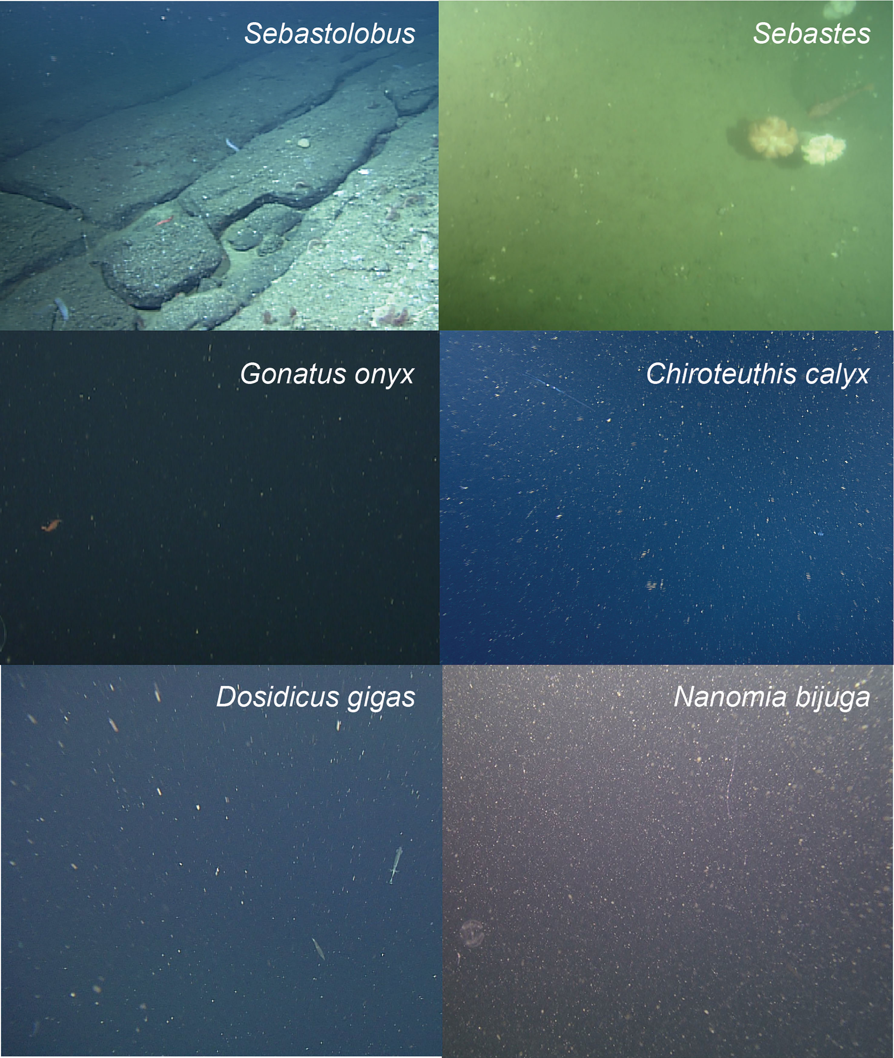
Figure 2 Typical images from FathomNet containing focal species. Focal species from Figure 1 shown in the context of more typical images from FathomNet. The focal class present in each image is noted in the upper right corner. Note complex and variable visual conditions, small size of objects of interest, clutter, and complex backgrounds. These conditions are typical in marine imagery collected for scientific sampling purposes.

We selected the six classes shown in Figures 1, 2 from the much larger set of classes available in FathomNet based on three criteria: (i) hundreds to thousands of human-generated labels were available for each class providing us with a sufficient number of labeled instances to explore performance of ML models under different partitions of the data, (ii) images of these classes were collected over a relatively broad spatial region and/or depth range compared to many other classes in FathomNet, allowing us to compare performance across spatial partitions of the data, and (iii) images of these classes were collected over many years, allowing us to partition the dataset temporally. Because searchable metadata, including depth and collection date, are included with the images in FathomNet, we were able to quickly create these partitions. As described in “Diagnosing and Improving Model Performance on New Data” below, we use these spatial and temporal partitions of the data to illustrate how ML models can fail when applied to new data, and how to diagnose and address such performance issues. We will return to this case study at the end of each section to provide a concrete example of each step involved in constructing and evaluating a machine learning pipeline.

3 Labeled imagery for training and evaluating models

3.1 Overview

The image-based ML methods that are currently most widely applied for marine science applications are based on supervised learning (Cunningham et al., 2008; Goodfellow et al., 2016). In supervised learning problems, the user provides a training dataset in which the desired output corresponding to a given input is specified for a set of examples. For object detection and classification problems, training data typically consist of a set of images (the image set) in which objects of interest are localized and identified by a human annotator. Labels (also sometimes referred to as “ground truths” or “annotations”) are standardized records of identity and, in some cases, spatial information describing what is contained within the image.

To train a supervised ML pipeline to perform image analysis automatically, one needs a suitable training dataset consisting of images and corresponding labels. A researcher has two choices for acquiring labeled data: manually create a set of labels to be used for training, or use images and labels from a pre-existing database (Table 2). At present, the number of publicly available annotated datasets containing marine imagery is relatively small, and the size and spatial, temporal, and taxonomic coverage of these datasets is still rather limited. In practice, this means that researchers typically need to create a new training dataset of annotated imagery de novo. This custom training set can then be used as a stand-alone training set or combined with images and labels from existing databases to fully train a ML model to carry out a specified task (Knausgård et al., 2021).

TABLE 2

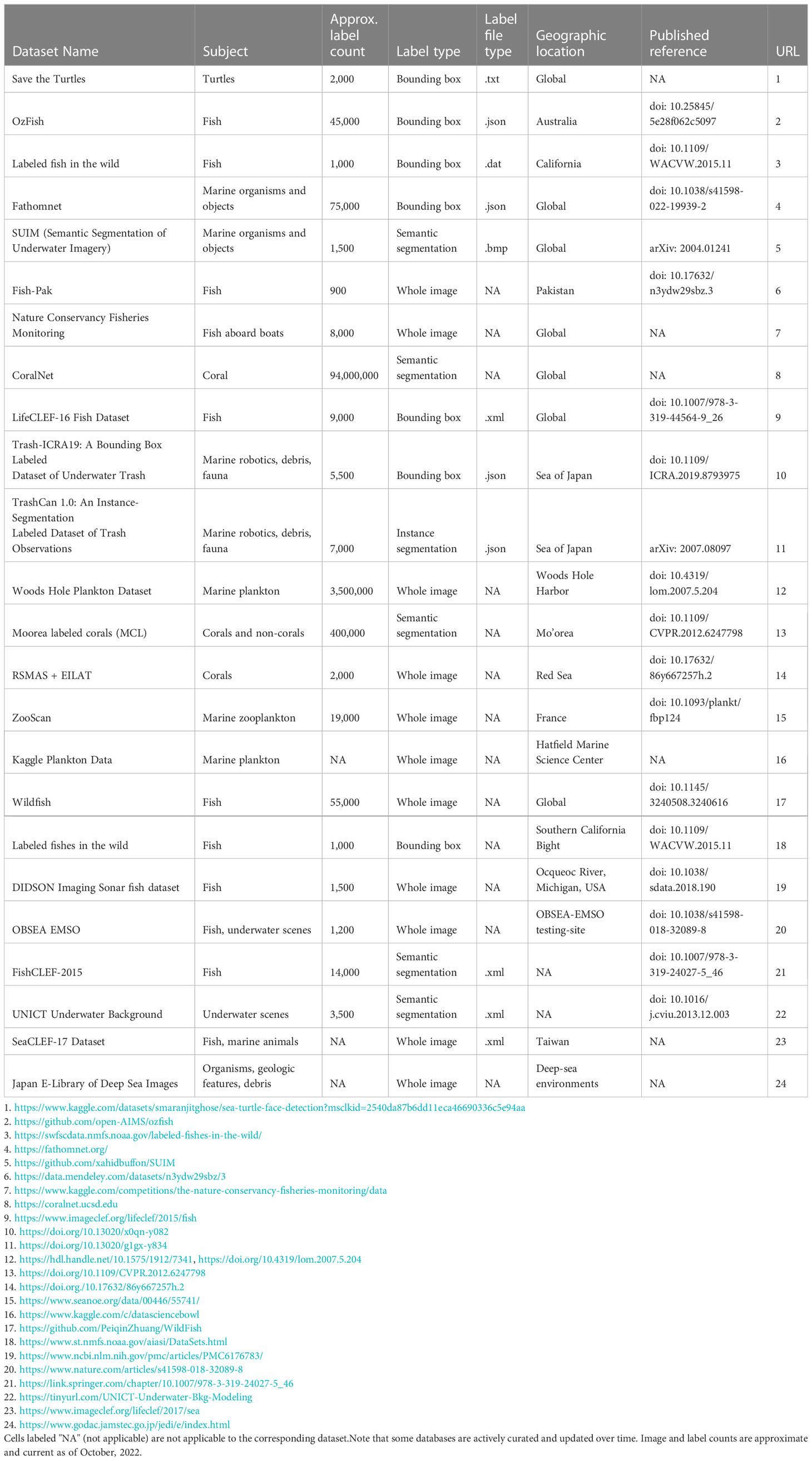
Table 2 Publicly available databases containing annotated images from marine environments.

3.2 Technical considerations

When building and working with training datasets, there are several issues a researcher should consider that can help determine which software tools are most useful, and how to best structure the labeling process to solve the desired image analysis task.

3.2 1 Label types

The most common method for creating new labels involves manual labeling of imagery (Mahajan et al., 2018; see Ji et al., 2019 for discussion of unsupervised methods). The type of label used depends on several considerations. The first consideration is the type of image analysis task that will allow the researcher to access the information they want to extract from the imagery (see “Defining the image analysis task” above).

If the objective is image classification, then labels consist of a class label assigned to each image in the training set (Figure 3A). For example, suppose the objective is to take in new images and to determine which images contain a target species and which do not. An appropriate training dataset would consist of a set of representative images from sampling cameras, each of which would be labeled by a human annotator as containing or not containing the target species.

FIGURE 3

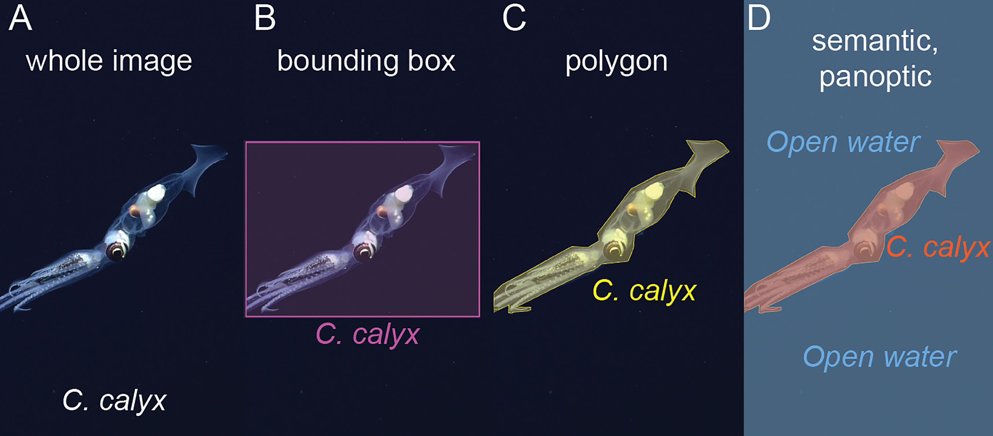
Figure 3 Examples of different label types. (A) Whole image labels assign a class to the entire image, in this case the squid species that occurs in the image. (B) Bounding box labels bound objects of interest within boxes and assign a class to each box. (C) Polygon labels bound each object of interest with a polygon and assign a class to each polygon. (D) Semantic segmentation assigns a class to each pixel in an image, in this case, pixels are labeled either “C. calyx” or “Open water” classes. In panoptic segmentation, pixels are assigned a class, and pixels belonging to the same instance of a given class are grouped together. Here, pixels assigned to the C. calyx class would be grouped into a single instance.

If the objective of image analysis is to localize and classify objects within an image, then manually generated labels must contain information about the locations and classes of objects of interest within an image. The most commonly used labeling formats for object detection are bounding box labels and polygon labels (Figures 3B, C). Bounding boxes are rectangular regions that enclose each object of interest and carry the appropriate class ID for the object (Figure 3B). Polygon labels, sometimes also referred to as “masks,” are enclosing polygons that outline an object of interest (Figure 3C). These too are associated with the class label of the object.

If the objective of image analysis is to assign the pixels in an image to distinct classes (i.e., semantic segmentation), for example to compute the fraction of the region captured in an image composed of different types of benthic cover, then labels must assign the pixels in an image to distinct classes (Figure 3D). This is typically done within labeling software by manually selecting the borders of local regions within the image and assigning a class to these regions. Some semi-automated “assisted methods” have been developed to aid in semantic labeling of images (e.g., Uijlings et al., 2020, “magic wand” tool in BIIGLE, Langenkämper et al., 2017).

Machine learning-based computer vision libraries such as Detectron 2 (Wu et al., 2019) and Deeplab v3+ (Chen et al., 2018) contain models that operate on an additional type of label referred to as a panoptic label. Panoptic labels include both class assignments for each pixel within an image and instance labels, so that the distinct pixels belonging to an individual instance of an object, for example, an individual squid, are grouped together (Figure 3D). We are not aware of past studies in marine science that have made use of panoptic labels, however, this type of labeling and segmentation could be useful in cases where a researcher wants to simultaneously characterize foreground objects of interest and background or substrate conditions.

3.2.2 Labeled data file formats

A variety of formats exist for storing manually generated labels. Unfortunately, there has been little standardization of the file formats used to encode labels of marine imagery, nor have researchers included consistent metadata within these files (Howell et al., 2019; Schoening et al., 2022). When creating new labels, we recommend choosing from among several formats that are most widely used in the computer vision community. These include YOLO text files, Pascal VOC XML files, and COCO (“common objects in context”, https://cocodataset.org/) Java Script Object Notation (JSON) formats. Pascal VOC and COCO formats both allow for convenient storage of metadata, making them attractive options.

3.2.3 Software for manually labeling imagery

A web search for the term “image labeling” will return many graphical user interface-based software tools designed to help users perform manual image labeling. In our experience, many of these tools work reliably, and are easy for human annotators to learn to use. Some widely-used, free labeling tools are CVAT (https://cvat.org), VGG Image Annotator (https://www.robots.ox.ac.uk/~vgg/software/via/), and Annotator J (https://biii.eu/annotatorj). Tools developed specifically for use in marine environments include BIIGLE (Langenkämper et al., 2017), VIAME (Richards et al., 2019), and EcoTaxa (Picheral et al., 2017; see Gomes-Pereira et al., 2016 for a review). These software tools are typically intuitive to use, but different tools have different capabilities that are important to understand when deciding which package to use for a given project. When selecting a software tool, there are four issues we suggest considering: (i) the speed and ease with which images can be loaded, labeled, and the labels exported; (ii) features the labeling tool offers such as convenient batch loading of images, zooming in and out, rotating images, assisted labeling, etc.; (iii) the label types the software allows (i.e., whole image labeling, bounding box labels, polygon labels, semantic labels, panoptic labels); and (iv) and labeled data file formats the software is capable of importing and exporting (e.g., Pascal VOC XML, COCO JSON).

3.2.4 Publicly available databases of annotated imagery from the field

In the computer vision literature, large, publicly available labeled image datasets such as ImageNet (14.2 million images; Russakovsky et al., 2015) and COCO (over 320,000 images; Lin et al., 2014) have been pivotal in driving the development of image-based ML methods. These datasets provide researchers with a source of data for quickly testing new model architectures, and for benchmarking and comparing new models using the same data sources. However, perhaps not surprisingly, these datasets contain relatively few images and label classes that are directly relevant to the use cases of interest to most marine scientists (Qin et al., 2016). Over the past decade, a number of curated open source databases containing labeled imagery from marine environments have begun to come online. The largest and most thoroughly curated of these are listed in Table 2. Depending on the specific problem a researcher is interested in addressing, these datasets may provide useful resources for model pre-training (Salman et al., 2016; Orenstein and Beijbom, 2017; Knausgård et al., 2021; Li et al., 2022), or if classes of interest are contained within one or more of these datasets, they may contain sufficient examples to train an initial model that can be deployed on new imagery and fine-tuned with new labels if needed.

3.2.5 Size of training set and balance among classes

An obvious question that arises when creating a training dataset is the question of how many images are required to achieve a desired level of performance. Several recent studies have sought to address this question for the tasks of instance segmentation (Ditria et al., 2020) and whole image classification (Piechaud et al., 2019; Villon et al., 2021). In these studies, performance metrics often begin to saturate at around 1,000 and 2,000 labels of a given class, beyond which point adding additional labeled data results in diminishing gains in performance. This saturation of performance around roughly 1,000 labeled instances per class is also consistent with other analyses of ML model performance on field imagery (e.g., Schneider et al., 2020 but see Durden et al., 2021). While the precise number of labels required to provide a desired level of performance is unlikely to follow a hard and fast rule, such numbers do provide ballpark estimates of the number of labeled instances per class one ought to have before expecting high performance from a ML model. It is worth noting, however, that many studies that report saturating performance as label count increases compute these metrics on test sets selected at random from the overall set of images used to train, test, and validate models (e.g., Ditria et al., 2020; Villon et al., 2021). As we will show later, the method of test set construction can have a major impact on measurements of model performance.

In practice, when constructing training sets, several factors are likely to influence the number of training labels available for each class. The first is the time and cost required to manually generate labels. Whole image classification by humans can be reasonably fast (e.g., 5 seconds per image, Villon et al., 2018); instance segmentation tends to be slower (e.g., 13.5 sec per image, Ditria et al., 2020); and more elaborate labeling such as panoptic is slower still (e.g., up to 20 minutes per image, Uijlings et al., 2020). How much time and money might it cost to create a labeled dataset? Assuming the per-image human instance labeling rate reported by Ditria et al. (2020), it would take 3.75 hours to label 1,000 images of a single class, which is not insignificant if objects of many different classes must be labeled. Katija et al. (2022) performed a more detailed valuation of the data contained within the initial release of FathomNet and estimated the initially uploaded dataset consisting of approximately 66,000 images to have taken over 2,000 hours of expert annotation time at a cost of roughly $165,000 for the labeling effort alone.

A second factor that influences the size of image datasets has to do with limited availability of images of rare classes. Even relatively large annotated image databases from the field typically contain many classes that are represented by far fewer than 1,000 instances (Schneider et al., 2020). Given the highly skewed distribution of species abundances documented in ecosystems around the world (McGill et al., 2007), it is simply expected that few species will be common, and most species will be far rarer. This distribution of species abundances is likely to result in image sets that contain relatively few training images of most species (Villon et al., 2021). When this is the case, using training routines (e.g., weighted penalization of errors, Schneider et al., 2020; hard negative mining, Walker and Orenstein, 2021) and ML pipelines that enhance performance on rare classes may be the only option. As an example of the latter, Villon et al. (2021) recently showed that, few-shot learning models can begin to saturate performance with tens of training examples per class rather than the thousand or more required by more conventional ML models. For this reason, development of few-shot learning methods is likely to be an important area of research in the coming years.

3.2.6 Scope of training imagery versus deployment imagery

One common source of underperformance of machine learning methods on new imagery can be traced to the range of conditions and class distributions present in the training set relative to new datasets on which the model is to be used. A good rule of thumb is to try to create a training dataset that spans the range of conditions you expect to sample when deploying the model on new imagery. For example, if you plan to use an image classifier on shallow water imagery collected from 30 distinct sampling locations across the daylight cycle, to the extent possible, train on imagery that contains the spatial and temporal variation inherent in this target use case. This does not necessarily mean labeling more imagery, but rather, labeling images that span the range of conditions expected when the model is applied to new image data. González et al. (2017) provide a detailed discussion of strategies for building a training and validation routines that yields reliable estimates of the future performance of a trained ML pipeline.

3.3 Case study: bounding box data from the FathomNet database with species- and genus-level class labels

As described above, our case study focused on six biological taxa detected in imagery collected in the Monterey Bay and surrounding regions of the coastal eastern Pacific. Images and corresponding labels for the classes used in our case study can be downloaded programmatically from FathomNet. Labels are downloadable from FathomNet in the widely-used COCO JSON format, which includes object bounding box instances corresponding to each image, along with their classes, and metadata associated with each image. Because we wished to apply a ML model called YOLO that does not accept COCO JSON as an input format, we had to convert labeled data to an admissible input format and create the necessary directory structure. Code to download and convert images and organize directories is provided at https://github.com/heinsense2/AIO_CaseStudy.

4 Selecting and training a machine learning model

4.1 Overview

After specifying an image analysis task and building a training dataset, the next step is identifying a particular machine learning model to train and test. Here, we are focused primarily on modern computer vision methods for automated analysis, many of which rely on deep learning – learning algorithms that involve the use of deep neural networks (DNNs). Deep learning is a form of representation learning, in which the objective is not only to use input data (e.g., an image) to make predictions (e.g., the class to which the image belongs), but also to discover efficient ways to represent the input data that make it easier to make accurate predictions (Bengio et al., 2013). Deep learning models are representation learning algorithms that teach themselves which features of an image are important for making predictions about the image. By training on a set of labeled images, these algorithms learn a mapping between raw pixel values and the desired output based on these features.

4.2 Technical considerations

Foundational work in deep learning demonstrated that networks that are good at representing features useful for prediction often share common structural features (LeCun et al., 2015), and this idea has fueled the use of deep neural networks with convolutional structure (Convolutional Neural Networks or CNNs), network pre-training, and other practices that help ensure that networks can quickly be trained to perform a target task on a new dataset, rather than having to be fully re-designed and trained de novo for each new application.

4.2.1 Selecting a machine learning model

The field of DNN-based models capable of performing image classification, object detection, and semantic segmentation is enormous, and expanding by the day. Table 3 provides a list of models that have shown promising results on imagery collected from either marine environments, or terrestrial environments that present similar challenges to those frequently encountered in marine environments (e.g., complex backgrounds, heterogeneous lighting, variable image quality, etc.) that is up to date as of this publication. Benchmarking sites (e.g., https://paperswithcode.com/sota/object-detection-on-coco) are another useful resources for tracking the most recent high-performing models on standard computer vision tasks.

TABLE 3

Table 3 Machine learning models applied to analysis of field imagery.

In a practical sense, choosing which ML model to use in any particular setting involves first determining which models can perform the target task (e.g., whole image classification vs. semantic segmentation). For any given target task, there will be many available models to choose from. We recommend researchers consider three things when choosing from among these models: (i) have previous studies evaluated and compared model performance? Has any study been done that applied a particular model in a similar setting with favorable performance? (ii) Is open-source code or a GUI-based implementation of the model available? If so, how easy does it appear to be to implement? Is it compatible with the computational hardware you have available? (iii) How many additional packages, software updates, and other back-end steps are required to be able to train and deploy a given model using new data? In our experience, perhaps the major hurdle associated with applying any given ML model to a new dataset is the time required to configure the software and system specifications necessary to run the model code. This “implementation effort” may ultimately dictate which model an end user ultimately selects. If a given ML model has been shown to exhibit good performance, but implementing that model requires significant knowledge of command-line interfaces, software package installers or dependencies, virtual environment management, hardware compatibility, or GPU programming, it may simply require too much invested time at the outset to be a viable option for most researchers.

4.2.2 Hardware implementation: CPU vs. GPU, local vs. cloud

Another decision a user must make when implementing ML pipelines is whether to run the computations involved in training, testing, and deploying the model on a computer’s central processing unit (CPU) or on the computer’s graphics processing unit (GPU). Among the technological developments that enabled widespread use of DNN models is software and hardware innovations that allow these models to be trained rapidly and in parallel using GPUs. The technical details of ML implementations on these two distinct types of hardware are discussed in Goodfellow et al. (2016) and Buber and Diri (2018). The advantage of training using a CPU is that any computer can, in principle, be used to perform training without the need for specialized hardware that some computers have and others lack. The disadvantage is that, in the absence of custom parallelization, training a DNN model of any depth using CPUs can be prohibitively slow. Fortunately, many consumer-grade workstations now ship with GPUs that are compatible with deep learning frameworks like PyTorch (Paszke et al., 2019) and Tensorflow (Abadi et al., 2016), and many universities and research institutes are investing in shared GPU clusters. Another option for accessing machines capable of training ML models is through cloud computing services such as Google Colab, Amazon Web Services, Microsoft Azure, and others. Free cloud services maybe a good option for researchers seeking to perform small pilot studies of ML model performance on their own datasets. Paid cloud services may be a particularly good option for researchers who wish to have access to many GPUs or powerful GPUs for relatively short periods of time, but who do not need or wish to manage their own local computing hardware.

4.3 Case study: object detection and classification with YOLO

Our case study task involves detecting objects of interest, along with a bounding box and class label for each object. We selected one of the most widely used object detection and classification pipelines, YOLO (“You-Only-Look-Once”, Redmon et al., 2016). YOLO is heavily used in industry and research applications, has fast deployment times relative to other deep architectures, and is relatively easy to use. Moreover, various versions of YOLO have been incorporated into more complex detection and classification pipelines that have shown promising results on marine imagery (e.g., Knausgård et al., 2021; Peña et al., 2021). For all analyses, we used initial weights provided in YOLO v5 from pre-training on the COCO dataset (https://github.com/ultralytics/yolov5 ). We selected the “small” network size as a compromise between network flexibility and the number of network weights that need to be estimated during training. Prior to training and testing, we reduced the resolution of images to 640 x 640 px (the impact of changing resolution is evaluated below). We included the five classes of squid and fish in our primary analysis, and reserved images of the siphonophore, N. bijuga, for a later analysis (see “Distractor classes” below).

We benchmarked training and deployment of YOLO v5 using both in-house hardware (a single workstation with four GPUs), and a cloud-based implementation. For the local hardware implementation, we used a Lambda Labs Quad workstation running Ubuntu 18.04.5 LTS and equipped with four NVIDIA GeForce RTX 2080 Ti/PCIe/SSE2 GPUs, each with 11,264 MB of memory. The machine also had a 24 Intel Core i9-7920X CPUs @2.90GHz with 125.5GiB of memory. Our cloud implementation used Google Colab (https://colab.research.google.com ), a cloud-based platform for organizing and executing Python programs using code notebooks (termed “Colab Notebooks”). Our cloud implementation made use of these resources using a Google Compute Engine backend with a single NVIDIA K80/Tesla T4 GPU with 16 GB of memory. In both local and cloud implementations, all models were trained for 300 epochs (or for fewer epochs when early stopping conditions were met) using all available GPUs. Run times on our local and cloud implementations were comparable, with the 4 GPU local machine performing slightly faster (mean of 19.1 sec per training epoch; 1.59 hours to complete 300 epochs) than the single GPU cloud implementation (mean of 26.8 sec per training epoch; 2.23 hours to complete 300 epochs). System specifications, software versions, training settings and all other details required to repeat our analyses are described in the accompanying code tutorial at https://github.com/heinsense2/AIO_CaseStudy.

5 Evaluating model performance

5.1 Overview

After training models, a final step in the model building process is to evaluate model performance. Many metrics are available for measuring the performance of ML models, and the most appropriate metric in any given application will depend both on the task the model is trained to execute (e.g., image classification vs. semantic segmentation), and the relative importance of different kinds of errors the model can make (e.g., false positives vs. false negatives), which must, of course, be determined by the researcher. Goodwin et al (2021) and Li et al (2022) provide approachable discussions of common metrics, along with formulae for computing them and the logic that underlies them. Tharwat (2020) provides a more technical account of classification metrics and their strengths and weaknesses. In very general terms, one typically wishes to evaluate the ability of the ML model to predict the correct class of an object, image, or subregion of the image, and, if the method provides spatial predictions about objects or semantic classes located in different parts of the image, one would like to know how accurate these spatial predictions are.

5.2 Technical considerations

For whole image classification, performance metrics seek to express the tendency of the model to make different kinds of errors when predicting classes. For example, suppose a researcher has 300 sea surface satellite images, and a model is trained to determine which images contain harmful algal blooms (HABs) and which do not (Henrichs et al., 2021). The classification accuracy of the model is the ratio of images that were assigned the correct class (HAB present vs. HAB absent) over the total number of images classified: (true positives + true negatives)/(total images classified). If the model correctly predicted 100 images that contained HABs, and correctly predicted 100 images that did not contain HABs, the accuracy is 200/300 = 0.67. Accuracy is an appealing measure because of its simplicity but it can be misleading, particularly when the dataset contains multiple classes and the relative frequency of classes differs (see discussion in Tharwat, 2020). Other widely-used metrics including precision, recall, and F1 score, were designed to capture other aspects of model performance, while avoiding some of the biases of classification accuracy. The precision of a classifier measures the fraction of positive class predictions that are correct. If the model classifies 130 images as containing HABs and 100 of these images actually contain HABs, the precision of the classifier is 100/130 = 0.77. Recall, sometimes also referred to as “sensitivity,” measures the ability of a model to detect all images or instances of a given class that are present in the dataset, thereby expressing how sensitive the model is to the presence of a class. If the classifier correctly classifies 100 images containing HABs but the dataset contains 160 images that contain HABs, the model’s recall is 100/160 = 0.63. The F1 score provides a composite performance measure that incorporates both precision and recall: F1 = 2 (precision x recall)/(precision + recall).

For methods that make spatial predictions, there is an additional question of whether the model’s spatial predictions are located in the right place. Among the most widely-used methods for measuring the spatial overlap between predictions and data this involves computing the spatial overlap between a prediction from the model and objects in the labeled image. This is often measured using the intersection-over-union (IoU): the intersection area of the predicted borders or bounding box of an object and the borders or bounding box of the label, divided by the total number of unique pixels covered by the bounding box and the label. Pairs in which the predictions precisely overlap labels will have equal intersection and union, giving an IoU value of one. Complete mismatches, partial spatial matches, or cases where the predicted and labeled bounding boxes differ in size will result in a union that exceeds the intersection and an IoU value less than one, with a minimum of zero when there is no overlap between predicted and observed bounding boxes.

In object detection and classification tasks, the added complication of predictions being spatial raises some questions about how one ought to compute the accuracy of class predictions. A standard practice is to consider a given bounding box a valid “prediction” if its IoU value exceeds some pre-specified threshold, which is often set arbitrarily at 0.5. For bounding box-ground truth pairs exceeding this threshold, one then evaluates performance using one or more of the same metrics applied in whole image classification (e.g., accuracy, precision, recall, F1 score, etc.). A widely-used metric is the mean average precision (mAP), which is most commonly calculated from the precision-recall curve as the average precision of model predictions over a set of evenly spaced recall values (Everingham et al, 2010), where the precision-recall curve represents model precision as a function of model recall across a range of values of a threshold parameter. The thresholds most often used are the box or instance confidence score and the IoU of predicted and labeled object detections. By default, YOLO v5 produces two measures of mean average precision: mAP@0.5, which is the mean average precision of the model assuming matches constitute all prediction-ground truth pairs with IoU >= 0.5, and a second measure, mAP@0.5:0.95, which is the arithmetic mean of average precision of the model computed across a range of threshold IoU values in the set, {0.50, 0.55,0.60,…,0.90, 0.95}. Different studies and machine learning software implementations compute mAP slightly differently, so ensuring that you understand how it is being computed is important when comparing predictions across studies or ML methods.

5.2.1 Cross validation and performance evaluation

When evaluating the performance of a model on test images held out during training, the exact values of performance metrics will depend on the particular subset of images used during testing. Because training, validation, and testing image sets are typically selected at random from the overall image set, random variability in exactly which images end up in training, validation, and test sets will invariably introduce stochasticity in performance estimates. One way to address this is to create several or even many random subsets of the overall image dataset into training, validation, and test sets. This is sometimes referred to as k-fold cross validation, where k denotes the number of training/validation/test splits included in the analysis. The objective of this type of cross validation is to provide more robust measures of performance by averaging over multiple random partitions of the data into training, validation, and testing sets.

5.2.2 Non-random partitioning and “out-of-domain” performance

In addition to cross validation using random partitions of the data, it is also becoming more common to evaluate model performance on non-random partitions of data into training/validation and test datasets (Schneider et al., 2020; Taori et al., 2020). Typically, this is done to produce test sets that are more representative of new data on which the ML pipeline is intended to be used. For example, if one wishes to train an image classifier to classify coral species from images (Wyatt et al., 2022), and this classifier is intended to be used at new locations in the future, one way to test its performance would be to divide the annotated imagery available into distinct spatial locations, and to construct the training and validation set from a subset of those locations, while holding out other locations that the model never sees during training. This type of model evaluation seeks to determine whether models are capable of performing well on images that may have very different statistics than the images on which they were trained. We will come back to this issue in the following section.

5.3 Case study: performance on object detection and classification of underwater imagery

In-domain performance on test imagery. Images of our target classes in FathomNet were collected at many different physical locations, and over decades of sampling (32 years spanning 1989-2021) using remotely operated vehicles equipped with a range of different types of imaging equipment. This led to an image set with complex and diverse backgrounds, highly variable visual conditions, and a wide range of image statistics (Figure 2) – characteristics that we expect will also be typical of medium- to long-term image datasets collected from other locations. Despite this variability, after training YOLO v5, we were able to achieve high object detection and classification performance on test imagery selected at random from the same spatial region or temporal period used to build the training set (Table 4 “in domain”). Mean average precision (mAP) of model predictions ranged from 0.67-0.95, and three classes had mAP values of 0.88 or above. Model F1 scores had an average value of 0.77, and three classes had F1 scores of 0.81-0.92. To put these performance metrics in context, Ditria et al. (2020) quantified the ability of citizen scientists and human experts to detect and classify a fish species (Girella tricuspidata) in images taken from shallow-water seagrass beds in Queensland, Australia. Citizen scientists and experts had mean F1 scores of 0.82 and 0.88, respectively. Comparing performance of YOLO v5 on our dataset to these benchmarks implies that our detection and classification results are in the same range as those of human annotators on a similar task.

TABLE 4

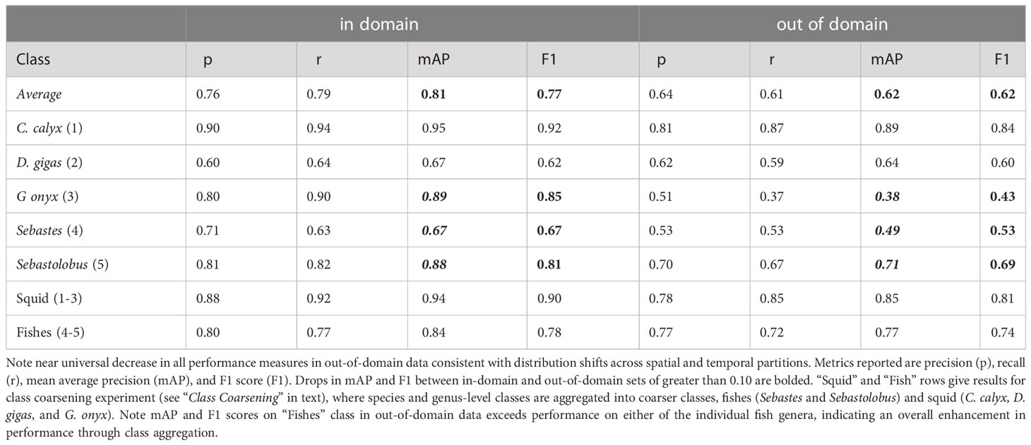
Table 4 Average performance of YOLO v5 object detection and classification on images selected at random from the same spatial or temporal partition used to build the training set (“in-domain”), or the partition held out (“out-of-domain”).

5.3.1 Out-of-domain performance: evidence for distribution shifts

As noted above, many researchers who wish to use machine learning pipelines to analyze imagery from the field often intend to use trained pipelines to analyze new imagery taken at later dates or different physical locations, rather than focusing solely on images taken from the same database used to construct the training set (Beery et al., 2018; Wyatt et al., 2022). To simulate this scenario, we performed a nonrandom, four-fold cross-validation procedure on the overall set of annotated imagery available on our classes of interest in FathomNet. This involved two different kinds of nonrandom partitioning of the dataset. The first was a temporal partition, in which we divided all annotated images of our focal classes into images collected prior to 2012, and images collected from 2012 through the present. This partitioning resulted in pre-2012 and post-2012 (2012 onward) image subsets. Splitting the data at 2012 yielded a similar number of labeled instances for most classes before and after the split. The second partition we performed was a spatial partition. Images from all sampling dates were pooled together. But for each class, we divided images either by depth or by latitude and longitude to ensure that images of each class were divided into distinct spatial “regions,” defined arbitrarily as region 1 and region 2. This temporal and spatial partitioning resulted in a four-fold partition of the data: two temporal sampling periods, and two spatial regions. We measured average performance over the four data partitions by training on one of the partitions and testing on the other (e.g., training on pre-2012 images and testing on post-2012 images).

Figure 4 and Table 4 shows the results of this analysis. Performance metrics were generally lower in the out-of-domain partition than in the partition from which training data were drawn (general trend of decreasing performance evident in Figure 4). This decrease in performance was particularly extreme for certain classes. For example, average mAP and F1 scores for the black-eyed squid, Gonatus onyx, were cut approximately in half – from 0.89 and 0.85, respectively, to 0.38 and 0.43 – when a model trained on one partition was deployed on the other. As previously suggested (Katija et al., 2022), these findings imply that distribution shift occur in the FathomNet dataset, and that these shifts can significantly degrade performance when models are trained on data from one set of locations or time periods and deployed on imagery from new locations or time periods. This phenomenon appears to be widespread in imagery collected from the field (Schneider et al., 2020; Wyatt et al., 2022).

FIGURE 4

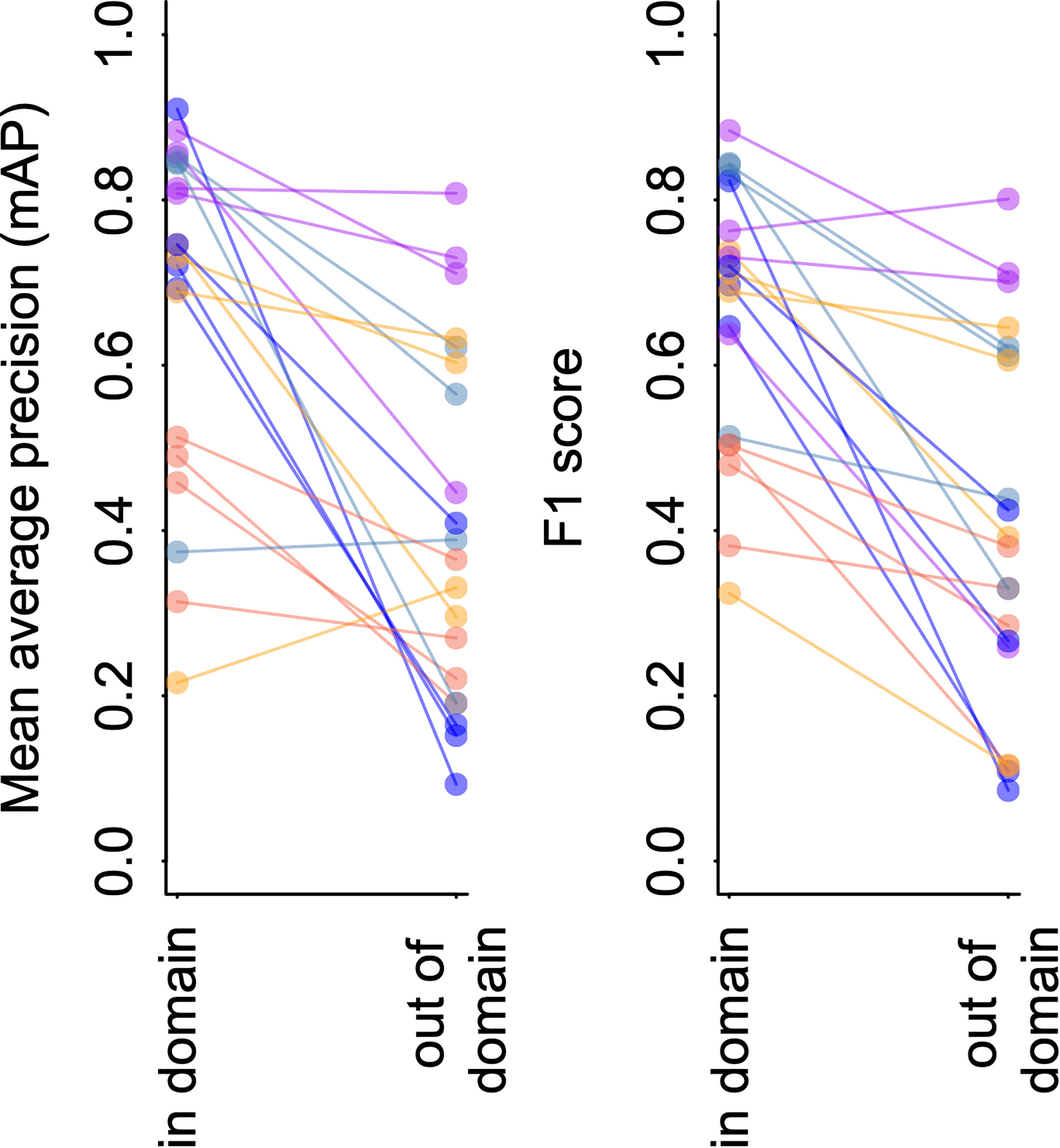
Figure 4 YOLO v5 model performance on imagery from FathomNet. Change in mean average precision (left) and F1 score (right) when a model is tested using out of sample data from the same spatial or temporal partition from which training data was selected (“in-domain”), and when the same model is tested using data from a different spatial or temporal partition (“out-of-domain”). Colors indicate different classes, and lines connect points from the same spatial or temporal partitioning of the data to indicate trends.

6 Diagnosing and improving model performance on new imagery

6.1 Overview

Although ML-based frameworks have shown impressive classification performance on imagery from marine systems (e.g., Kyathanahally et al., 2022), inevitably, all models make errors. Moreover, the degree to which a previously trained model makes errors when applied to new image datasets can change over time as new imagery changes relative to the original dataset used to perform training. Therefore, one key step in building and maintaining a ML pipeline for automated image analysis is diagnosing performance problems and finding ways to fix them (Norouzzadeh et al., 2018). In this section, we address issues that can degrade performance of a ML pipeline, and suggest approaches for remedying these issues. Many such issues can be traced back to the problem of distribution shift (Beery et al., 2018; Schneider et al., 2020; Taori et al., 2020). A distribution shift occurs when the imagery on which a ML pipeline is trained differs in some systematic way from the imagery on which the pipeline is deployed – that is, the new imagery the ML method is being used to analyze. The term “distribution shift” refers to a generic set of differences that may occur between one set of images (the “in-domain” set) and another (the “out-of-domain” set), including things like differences in lighting, camera attributes, image scene statistics, background clutter, turbidity, and the relative abundances and appearances of different classes of objects (Taori et al., 2020; Scoulding et al., 2022; Wyatt et al., 2022).

Many existing ML methods perform poorly under distribution shifts without careful training interventions (Beery et al., 2018; Schneider et al., 2020; Taori et al., 2020). Despite this, human labelers exhibit similar performance on original and distribution shifted datasets (Shankar et al., 2020), suggesting that distribution shifts do not reduce the information needed to accurately identify objects per se, but rather that the structure and training of ML models cause them to fail on distribution shifted imagery (Taori et al., 2020). Given that distribution shifts are documented here (Figure 4, Table 4), and in past studies of imagery from the field (e.g., Beery et al., 2018; Schneider et al., 2020; Katija et al., 2022), a natural question is whether there are steps that can be taken to reduce their effects on model performance.

6.2 Technical considerations

A wide array of methods have been proposed to improve the performance of ML models on new imagery that is distribution shifted relative to training images. These range from training interventions like digitally altering (i.e., “augmenting”) training imagery to destroy irrelevant features that can result in overtraining (Bloice et al., 2019; Buslaev et al, 2020; Zoph et al., 2020), to the use of more robust inference frameworks such as ensemble models, which combine predictions of multiple machine learning models (Wyatt et al., 2022). To provide a sense for how some of these methods work, we applied a suite of training interventions to our case study dataset.

Image augmentation is a widely used method for improving model performance on out-of-sample and out-of-domain imagery (Bloice et al., 2019; Buslaev et al, 2020; Zoph et al., 2020). Image augmentation involves applying random digital alterations of training imagery during the training process to help avoid over-fitting ML models to specific nuances of training imagery that are not useful for identifying objects of interest in general. Augmentation of training images is used by default in many ML pipelines (including YOLO v5) as part of the training process, but augmentation parameters are often tunable, so having some understanding of how different types of augmentation affect performance on field imagery is useful.

Increasing image resolution is another straightforward training intervention. Due to the computational and memory demands of training DNN-based ML models, it is common to reduce image resolution during training, testing, and deployment (e.g., Kyathanahally et al., 2022). However, if objects of interest constitute relatively small regions of the overall image (e.g., Figure 2), reducing resolution can coarsen or destroy object features that can be important for detection and classification. The loss or degradation of these features during training and deployment, mean that they cannot be used to accurately detect and classify objects in new imagery that is distribution shifted relative to the training set. It may, therefore, be beneficial in some applications to maintain higher image resolutions during training and deployment.

Training using background imagery is another intervention that is relatively easy to implement. While it can be costly to label new imagery for the reasons discussed above, it can be relatively cheap to identify “background images,” defined simply as images that do not contain objects of interest. Training a ML model by deliberately including background imagery in the training set has been proposed as one method for helping models to better generalize to new image sets (Villon et al., 2018).

A fourth type of intervention is known as class coarsening. Intuitively, objects that are visually similar are likely to be harder to discriminate than are objects that look very different. Given this, one potential solution to improve model predictions under distribution shifts is to coarsen class labels in a way that results in similar looking classes being aggregated into a single super-class (Williams et al., 2019; Katija et al., 2022). In biological applications, this may result in aggregating classes with finer phylogenetic resolution (e.g., species or genus-level classes) into classes with coarser resolution (e.g., family or order-level classes or coarse species groups). For instance, rather than requesting individual species of sea fan and corals, one might simply specify “sea fans” and “corals” as classes (but see Howell et al., 2019 for a discussion of the need to aggregate with care). Whether this is a suitable training intervention obviously depends on the ultimate goal of the image analysis and whether coarser class labels are acceptable.

A final intervention we consider is training on images that include objects in distractor classes. The definition of the term “distractor” in the computer vision literature has varied (e.g., see Das et al., 2021 vs. Zhu et al., 2018). Here, we define a distractor class as a class of object that shares visual characteristics with a target class and could reasonably be confused with the target class during classification. This working definition is consistent with the way the term “distractor” is used in the visual neuroscience literature (e.g., Bichot and Schall, 1999). When training ML models to detect a certain class or small set of classes, it is common to train models using labels of only the class or classes of interest. However, if distractor classes are regularly present in new imagery, they can degrade model performance. Deliberately including images of distractor classes in the training set is a form of adversarial training that may improve model performance when distractor classes occur in new imagery.

In addition to these simple training interventions, a variety of other solutions to improve model robustness on new imagery have been proposed. These include the use of ensemble models, where predictions are derived not from just one deep neural network, but from many networks whose predictions are combined to make an overall class prediction (Wyatt et al., 2022), adversarial training, sometimes also called “active learning,” in which models are re-trained with images on which they previously made errors (Mathis et al., 2020), training on synthetic data (Schneider et al., 2020), and stratified training in which the relative abundance of classes in the training set are modified by excluding or including extra examples of one class or another (Schneider et al., 2020). There are related methods that seek instead to analyze the output of automated systems at the sample level, rather than the individual level, to correct errors and detect changes in new domains (González et al., 2019; Walker and Orenstein, 2021). We refer the reader to the research cited in this section, and to Taori et al. (2020); Schneider et al (2020) and Koh et al. (2021) for further reading on methods for improving performance under distribution shifts.

6.3 Case study: training interventions and performance on out-of-domain imagery

6.3.1 Image augmentation

To test whether and how augmentations might improve model performance on new imagery, we applied three kinds of augmentation to images during training: orientation augmentations, in which the training image and corresponding bounding box is scaled or flipped by a random amount, color space augmentations, in which the color attributes of the training image are randomly perturbed during training, and mosaic augmentation, in which sets of training images from the training set are randomly selected, cropped, and recombined to form a new composite “mosaic” image used in training. We tested the impact of each of these augmentation types by starting with all of them active, then dropping one augmentation type at a time. For each of these augmentation “treatments,” we computed performance metrics on the out-of-domain testing set, averaging over all four partitions of the data. Augmentation parameters and parameter values are defined in the case study code accompanying this manuscript.

Applying no augmentations at all resulted in the poorest performance (Table 5), whereas the best performance occurred when all augmentations were applied. However, the effects of augmentations were highly variable among different partitions of the data, and among classes. These results suggest that augmentation may indeed be a way to improve generalization on new imagery, but that effect of augmentation may differ from one class to another. We did not observe a systematic decrease in performance under any augmentation scheme. However, Tan et al. (2022) recently reported such decreases in performance in the context of marine benthic imagery, emphasizing that it is important to choose augmentation routines with care.

TABLE 5

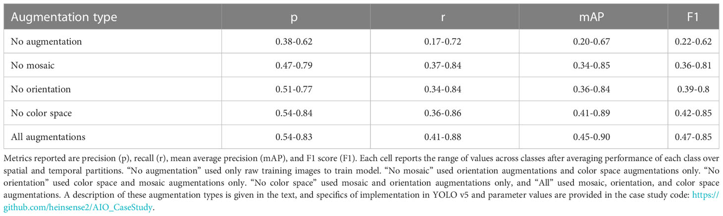
Table 5 Effect of image augmentation on performance of YOLO v5 on out of domain set.

6.3.2 Image resolution

To explore the impact of changing image resolution in our case study, we modified the default resolution specified in YOLO v5 (640 px x 640 px) to a higher resolution (1280 px x 1280 px). Between 91% and 98% of images available in FathomNet for each class have a resolution equal to or greater than 640 pixels along at least one axis. Images with resolution lower than 1280 x 1280 were loaded at full resolution and padded at the borders to reach the desired training resolution. Effects of increased image resolution were not large. For example, the average change in mean average precision on out-of-domain data across the four partitions was 0.04, and the largest performance increase was only 0.05 (for G. onyx), while performance on C. calyx actually dropped slightly when we used higher resolution imagery. It is worth noting that differences in resolution between training and testing data can cause degraded performance (Recht et al., 2019), which may have contributed to a lack of improvement in performance in some of the partitions (e.g., pre-2012 vs. post-2012 splits, for which image resolution systematically differed).

6.3.3 Training on background imagery

To test whether training on background imagery could improve out-of-domain performance, we re-trained YOLO v5 using the post-2012 partition as a training set, but we also included background images from the pre-2012 and post-2012 partitions in the training imagery. Including background imagery improved performance on all classes (Table 6), with the largest increases in performance for Dosidicus gigas and Gonatus onyx, the classes with the fewest labels in the training set (n = 42, and n = 84 labeled instances, respectively).

TABLE 6

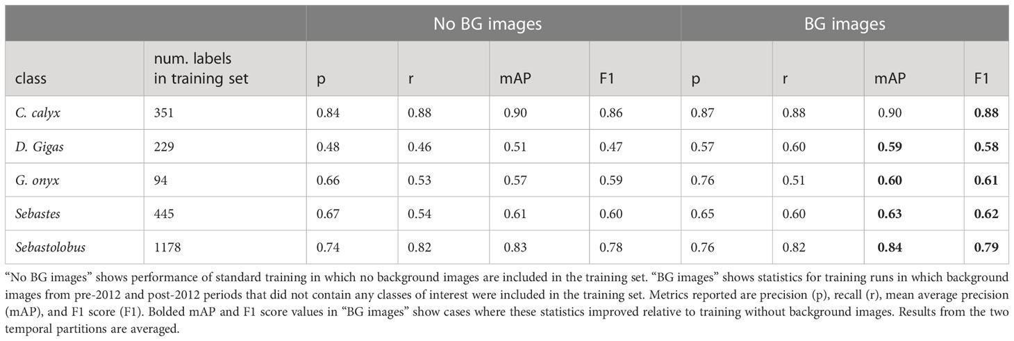
Table 6 Effect of including background imagery on performance of YOLO v5 on out of domain imagery (temporal partitions).

6.3.4 Class coarsening

To explore whether class coarsening improved performance under distribution shifts, we coarsened class labels from the species (Gonatus onyx, Chiroteuthis calyx, and Dosidicus gigas) and genus level (Sebastes and Sebastolobus) to the coarse categories of squids and fishes. Table 4 shows performance of YOLO v5 when trained and tested on these coarser classes. As expected, coarsening classes resulted in a smaller average drop in model performance when models were applied to out-of-domain data. For the squid class, out-of-domain performance was higher than for any individual class in the fine class model except for C. calyx (class for which the model had the highest performance). Out-of-domain performance for the fish class was higher than performance on either of the individual fish genera in the analysis where genera were treated as separate classes.

6.3.5 Training with distractor classes

To quantify the impact of training with distractor classes on model performance, we restricted our analysis to two classes: the swordtail squid, Chiroteuthis calyx, and the siphonophore, Nanomia bijuga. In particular, we sought to determine whether a trained ML model could discriminate images of juvenile swordtail squid in an image set containing images of juvenile C. calyx and imagery of N. bijuga, a distractor class that is a mimicked both morphologically and behaviorally by juvenile C. calyx (Burford et al., 2015). Because the spatial distributions and habitat use of these two species overlap, a researcher interested in C. calyx would likely need to contend with images containing N. bijuga, either by itself or in the same image as the target class C. calyx (e.g. as in Figure 1F). A naïve approach for training a ML model to detect juvenile C. calyx, would be to train only on images of this target class, and then to deploy the model on new images containing one or both of the two classes.

Table 7 shows performance of YOLO v5 trained to detect juvenile C. calyx using this naïve approach. Mean average precision is relatively poor as are precision and recall scores (e.g., mAP = 0.54). Moreover, 22% of the instances of N. bijuga in test data were erroneously classified as C. calyx, indicating that the model often mistook the distractor class for the target class. To determine whether training on both the target and distractor class could help remedy this issue, we re-trained YOLO v5 with a training set containing labeled imagery of both juvenile C. calyx and N. bijuga. We then applied this model to test imagery. Training on both classes resulted in a pronounced increase in all performance metrics to levels that match or exceed reported performance of human labelers in similar tasks (precision = 0.86, recall = 0.9, mAP = 0.87). Moreover, despite the strong morphological resemblance between N. bijuga and juvenile C. calyx (Figure 1F), the model trained on both classes never classified new images of C. calyx as N. bijuga or vice versa (0% misclassification rate). A third approach to improving model performance in the presence of distractor classes that is less costly than manually labeling distractor classes is to include in the training set images that contain the distractor, but to treat these as unlabeled “background” imagery. That is, if an image contains only the distractor class, it would be included in the training set with no instance labels. To test this approach, we used the same images of C. calyx and N. bijuga used to train the two-class model, but we included no labels for the N. bijuga class. Performance using this approach was only slightly lower than performance of the model trained on labels of the distractor (Table 7), indicating that such training be a viable alternative to building a full dataset containing labels for distractors as well as the target class.

TABLE 7

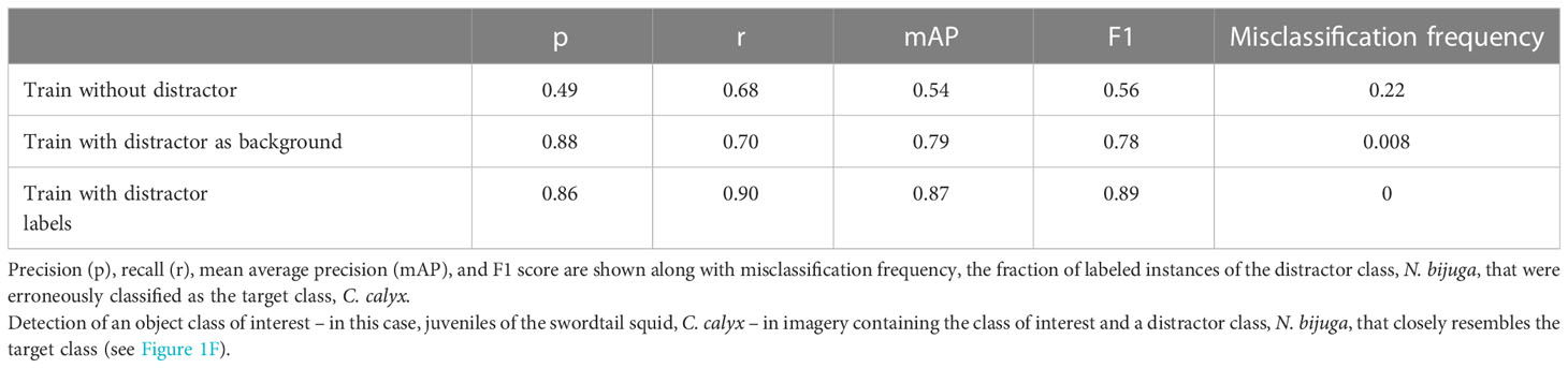
Table 7 Effects of distractor class on model performance.

6.3.6 Summary of training interventions and their effects on performance on new imagery

The image set and number of classes used in our case study was intentionally limited, so our findings should also be taken with this in mind. Overall, we found that image augmentation (improvement in mAP of 0.18-0.25, F1 of 0.04-0.25), and class coarsening (average improvement in mAP of 0.21-0.25, F1 of 0.13-0.19) provided improvements in performance on new imagery in all or most classes in the dataset. Training distractors also resulted in large improvements in performance for the target class used in the distractor analysis (improvement in mAP of 0.25-0.33, F1 of 0.22-0.33). The impact of training on background imagery was more variable, but still resulted in overall improvements in performance for most classes (improvement in mAP of 0-0.08, F1 of 0.01-0.11). Training and deploying the model on high-resolution imagery (as opposed to images with reduced resolution) had the smallest and most variable effect on performance (e.g., change in mAP of -0.04-0.05), but this should be taken with the caveat that our image set consisted of a mix of high- and low-resolution imagery, and that resolution mismatches between training and testing data can sometimes result in poor performance (Hendrycks and Dietterich, 2019; Recht et al., 2019).

7 Recommendations and conclusions

Image-based machine learning methods hold tremendous promise for marine science, and for the study of natural systems more generally. These methods can vastly accelerate image processing, while also greatly lowering its costs (Gaston & O'Neill, 2004; MacLeod et al., 2010; Norouzzadeh et al., 2018; Katija et al., 2022). In doing so, they could fundamentally change the spatial coverage and frequency of sampling achieved by field research and monitoring efforts. Our objective in this work has been to provide a guide for researchers who may be new to these methods, but wish to apply them to their own data. If image-based machine learning methods are to be more widely adopted and fully exploited, the current high barrier to entry associated with these methods must be lowered (Crosby et al., 2023). We therefore conclude with four suggestions for the research community that we believe could help expand the use of, and access to image-based machine learning tools across marine science.

7.1 Open sharing of labeled image datasets from the field

At present, the ability of researchers to test and engineer ML methods relevant to the tasks marine scientists want to perform on imagery is constrained by the limited publicly available data for training and testing these methods. Thus, among the most important steps that can be taken to improve ML models for use in the marine domain, is to increase the availability, coverage, quality, and size of domain-relevant labeled image datasets, as well as the standardization of label formats and class naming conventions across those datasets. As Table 2 shows, available datasets focus rather heavily on tropical fishes, benthic habitats, coral, and marine phytoplankton, whereas imagery of other kinds of objects of interest and imagery from other habitats is not as well represented. Researchers who generate manually labeled image datasets in the course of their work would contribute much to the community by making those datasets available in a form that is easily readable by ML pipelines. The issue of readability extends beyond using standard file formats and labeling methods, it also means using class naming conventions that are interpretable and useable by other researchers in the future (Schoening et al., 2022). Idiosyncratic class definitions – for example the use of project- or institution-specific operational taxonomic units – are one major factor that limits the utility of many existing image datasets (Howell et al., 2019). The more standardized and interoperable such datasets become, the more tractable it will be to fully exploit the tremendous volume of ocean imagery currently being collected (Schoening et al., 2022).

Good methods for releasing and publicizing datasets include stand-alone publications (e.g., Saleh et al., 2020; Ditria et al., 2021), publication of datasets as part of standard research publications (e.g., Sosik & Olson, 2007), or contributing datasets to existing open image repositories such as FathomNet (Katija et al., 2022) and CoralNet (Williams et al., 2019). Of course, constructing labeled image datasets requires funding, domain expertise, and a significant commitment of personnel time. It is therefore crucial that researchers who generate such datasets and the funding sources that support them receive credit. This will involve a shift in perspective from viewing labeled imagery as simply a means to an end, to viewing these kinds of datasets as valid research products in their own right (Qin et al., 2016; Ditria et al., 2021; Koh et al., 2021). Fortunately, this shift in perspective is already beginning to occur, and we expect funding agencies, tenure and promotion committees, and the broader research community will continue to move in the direction of recognizing the value of producing and sharing high-quality labeled image datasets.

7.2 Sharing of open source code for repeating analyses

A second recommendation is aimed at researchers who are developing and testing ML methods for analyzing imagery from the field. It is now commonplace among the larger computer vision community for preprints, conference publications, and journal publications to include links to code repositories that contain the code necessary to repeat analyses. We encourage researchers who are developing ML methods to solve problems in marine science to follow this same practice. Providing the code that accompanies work described in publications can accelerate research. While newer studies are beginning to follow this practice, it is still not as widespread among researchers working in marine science as it is in the broader machine learning community (Table 3). Code can be efficiently shared, for example, through GitHub repositories or through “model zoo” features of existing image repositories (e.g., https://github.com/fathomnet/models). The machine learning community is adopting standards to further enable model sharing via model and dataset cards, resources that allow users to understand at a glance what they are downloading (Mitchell et al., 2019). Applying similar standards in the marine science community would help ensure that code and accompanying data is structured and benchmarked consistently across studies.

7.3 Develop and adopt standards for model evaluation that accurately capture performance in common use-cases

At present, there has been little standardization of model performance metrics reported in papers that apply image-based machine learning to problems in marine science. Different papers report different metrics that often include just one or a few of the performance measures described in “Evaluating model performance” above. The most commonly reported metric across studies is classification accuracy (Table 3), but, as noted above, this metric is subject to biases that inherently make comparisons across studies problematic (Tharwat, 2020). Another less obvious issue is that different studies compute performance metrics from test data sets that are built in very different ways. For example, some studies compute performance from a single random partition of the data into training, validation, and test sets. Others perform several random partitions of the overall dataset using a k-fold cross-validation procedure. Others still report true out-of-domain statistics computed on test data from specific locations or time periods that were held out during training (see Table 3). The manner in which test imagery is selected (e.g., at random from in-domain data vs. from out-of-domain data) can have a major impact on performance measures, and any fair comparison between methods clearly requires that performance statistics of competing methods be computed in the same way.

In the end, the most appropriate performance measures will be the ones that best reflect how a model will perform at the task for which it is ultimately intended to be used (González et al., 2017). At the same time, adopting a standard will likely be necessary if performance is to be compared among studies. To achieve this compromise, it will be productive for the community of developers and users of image-based machine learning methods to begin a conversation about the most appropriate standards for evaluating models and comparing model performance among studies, with the goal of identifying metrics that meet the needs of researchers. One potentially fruitful question that could guide this conversation is how the standard performance measures used to evaluate machine learning models (e.g., precision, recall, F1) relate to widely-used statistics scientists often want to compute using image data (e.g., abundance, species richness, measures of ecological community composition, Durden et al., 2021).

7.4 Develop open source, GUI-based applications that implement full image analysis pipelines

A full pipeline for applying image-based ML models in a versatile way requires software to carry out tasks ranging from image labeling and curation to visualizing results of ML model predictions. The transition from largely manual analysis of imagery to ML-based automated analysis is already taking place in other fields, and the availability of free, GUI-based, and actively maintained software packages that integrate all of these tasks has helped facilitate this transition. We point to the DeepLabCut package (Mathis and Mathis, 2020; Mathis et al., 2020, https://github.com/DeepLabCut/DeepLabCut) developed for the study of neuroscience and quantitative behavior from laboratory videos as a potent example of how easy-to-use software can rapidly increase use of ML methods within a field. Although some efforts are underway to produce similar “all-in-one” packages for analyzing imagery from marine environments (e.g., the VIAME project; Richards et al., 2019), and several application-specific packages are already in use (e.g. CoralNet, Lozada-Misa et al., 2017; ReefCloud, ReefCloud, 2021), most research groups that apply image-based ML models to data from the field still use custom software pipelines that often combine many packages and software modules (see references in Table 3). We believe that creating software architectures that allow users to easily build their own annotated image libraries and to quickly test and evaluate performance of a suite of widely used ML methods may be the single biggest step that can be taken to encourage broader adoption of these methods in marine science.

8 Conclusions

The evolving research needs of the marine science community will undoubtedly lead to new priorities, and we do not intend these suggestions to be exhaustive. Yet, we believe these steps would go a long way toward making image-based machine learning easier to use, more reliable, and more accessible. As we move toward these goals, it will be crucial to create an open dialogue between researchers who are developing and testing image-based ML methods and researchers who are collecting, labeling, and analyzing imagery from the field. Such a dialogue will help fuel the development of novel methods that empower marine scientists to use machine learning to study the ocean in ways that were never before possible.

Author contributions

All authors designed research. All authors performed research. All authors wrote manuscript. All authors contributed to the article and approved the submitted version.

Funding

This work was supported by National Science Foundation grant IOS-1855956 and REU supplement to AMH, and National Science Foundation grant EF-2222478 to AKF and AMH. This work was produced as a result of the AI for the Ocean undergraduate interdisciplinary training program in science and technology.

Acknowledgments

We thank B. Schlining, B. Martin, and M. Gil for useful discussions, advice, and technical support that improved this manuscript.

Conflict of interest

The authors declare that the research was conducted in the absence of any commercial or financial relationships that could be construed as a potential conflict of interest.

Publisher’s note

All claims expressed in this article are solely those of the authors and do not necessarily represent those of their affiliated organizations, or those of the publisher, the editors and the reviewers. Any product that may be evaluated in this article, or claim that may be made by its manufacturer, is not guaranteed or endorsed by the publisher.

References

Abadi M., Barham P., Chen J., Chen Z., Davis A., Dean J., et al. (2016). “{TensorFlow}: a system for {Large-scale} machine learning,” in 12th USENIX symposium on operating systems design and implementation (OSDI 16) (Savannah, GA, USA: USENIX Association). 265–283.

Google Scholar

Allken V., Handegard N. O., Rosen S., Schreyeck T., Mahiout T., Malde K. (2019). Fish species identification using a convolutional neural network trained on synthetic data. ICES J. Mar. Sci. 76, 342–349. doi: 10.1093/icesjms/fsy147

CrossRef Full Text | Google Scholar

Bamford C. C. G., Kelly N., Dalla Rosa L., Cade D. E., Fretwell P. T., Trathan P. N., et al. (2020). A comparison of baleen whale density estimates derived from overlapping satellite imagery and a shipborne survey. Sci. Rep. 10 (1), 1–12. doi: 10.1038/s41598-020-69887-y

PubMed Abstract | CrossRef Full Text | Google Scholar

Beery S., Agarwal A., Cole E., Birodkar V. (2021). The iwildcam 2021 competition dataset. arXiv preprint arXiv 2105.03494. doi: 10.48550/arXiv.2105.03494

CrossRef Full Text | Google Scholar

Beery S., van Horn G., Perona P. (2018). “Recognition in terra incognita,” in European Conference on Computer Vision (ECCV). Lecture Notes in Computer Science (Cham: Springer) 456–473. doi: 10.48550/arXiv.1807.04975

CrossRef Full Text | Google Scholar

Beijbom O., Edmunds P. J., Roelfsema C., Smith J., Kline D. I., Neal B. P., et al. (2015). Towards automated annotation of benthic survey images: variability of human experts and operational modes of automation. PloS One 10 (7), e0130312. doi: 10.1371/journal.pone.0130312

PubMed Abstract | CrossRef Full Text | Google Scholar

Bengio Y., Courville A., Vincent P. (2013). Representation learning: a review and new perspectives. IEEE Trans. Pattern Anal. Mach. Intell. 35 (8), 1798–1828. doi: 10.1109/TPAMI.2013.50

PubMed Abstract | CrossRef Full Text | Google Scholar

Bichot N. P., Schall J. D. (1999). Saccade target selection in macaque during feature and conjunction visual search. Visual Neurosci. 16 (1), 81–89. doi: 10.1017/S0952523899161042

CrossRef Full Text | Google Scholar

Bloice M. D., Roth P. M., Holzinger A. (2019). Biomedical image augmentation using augmentor. Bioinformatics 35 (21), 4522–4524. doi: 10.1093/bioinformatics/btz259

PubMed Abstract | CrossRef Full Text | Google Scholar

Buber E., Diri B. (2018). “Performance analysis and CPU vs GPU comparison for deep learning,” in 6th International Conference on Control Engineering & Information Technology (CEIT), Istanbul, Turkey. 1–6. doi: 10.1109/CEIT.2018.8751930

CrossRef Full Text | Google Scholar

Burford B. P., Robison B. H., Sherlock R. E. (2015). Behaviour and mimicry in the juvenile and subadult life stages of the mesopelagic squid chiroteuthis calyx. J. Mar. Biol. Assoc. United Kingdom 95 (6), 1221–1235. doi: 10.1017/S0025315414001763

CrossRef Full Text | Google Scholar

Buslaev A., Iglovikov V. I., Khvedchenya E., Parinov A., Druzhinin M., Kalinin A. A. (2020). Albumentations: fast and flexible image augmentations. Information 11 (2), 125. doi: 10.3390/info11020125

CrossRef Full Text | Google Scholar

Chapelle O., Haffner P., Vapnik V. N. (1999). Support vector machines for histogram-based image classification. IEEE Trans. Neural Networks 10 (5), 1055–1064. doi: 10.1109/72.788646

CrossRef Full Text | Google Scholar

Chegini H., Beltran F., Mahanti A. (2022). Designing and developing a weed detection model for California thistle(TOIT). ACM Trans. Internet Technol.

Google Scholar

Chen L. C., Zhu Y., Papandreou G., Schroff F., Adam H. (2018). “Encoder-decoder with atrous separable convolution for semantic image segmentation,” in Proceedings of the European conference on computer vision (ECCV). Lecture Notes in Computer Science (Cham: Springer) 801–818.

Google Scholar

Crosby A., Orenstein E. C., Poulton S. E., Bell K. L., Woodward B., Ruhl H., et al. (2023). “Designing ocean vision AI: an investigation of community needs for imaging-based ocean conservation,” in Proceedings of the 2023 CHI Conference on Human Factors in Computing Systems. (New York, NY, USA: Association for Computing Machinery) 1–16.

Google Scholar

Cunningham P., Cord M., Delany S. J. (2008). “Supervised learning,” in Machine learning techniques for multimedia. cognitive technologies. Eds. Cord M., Cunningham P. (Berlin, Heidelberg: Springer). doi: 10.1007/978-3-540-75171-7_2

CrossRef Full Text | Google Scholar

Das R., Wang Y. X., Moura J. M. (2021). “On the importance of distractors for few-shot classification,” in Proceedings of the IEEE/CVF International Conference on Computer Vision, Montreal, QC, Canada. 9030–9040. doi: 10.1109/ICCV48922.2021.00890

CrossRef Full Text | Google Scholar

Ditria E. M., Connolly R. M., Jinks E. L., Lopez-Marcano S. (2021). Annotated video footage for automated identification and counting of fish in unconstrained seagrass habitats. Front. Mar. Sci. 8, 629485. doi: 10.3389/fmars.2021.629485

CrossRef Full Text | Google Scholar

Ditria E. M., Lopez-Marcano S., Sievers M., Jinks E. L., Brown C. J., Connolly R. M. (2020). Automating the analysis of fish abundance using object detection: optimizing animal ecology with deep learning. Front. Mar. Sci. 429. doi: 10.3389/fmars.2020.00429

CrossRef Full Text | Google Scholar

Drew E. A. (1977). A photographic survey down the seaward reef-front of aldabra atoll. Atoll Res. Bull. 193, 1–7. doi: 10.5479/si.00775630.193.1

CrossRef Full Text | Google Scholar

Durden J. M., Hosking B., Bett B. J., Cline D., Ruhl H. A. (2021). Automated classification of fauna in seabed photographs: the impact of training and validation dataset size, with considerations for the class imbalance. Prog. Oceanography 196, 102612. doi: 10.1016/j.pocean.2021.102612

CrossRef Full Text | Google Scholar

Durden J. M., Schoening T., Althaus F., Friedman A., Garcia R., Glover A. G., et al. (2016). “Perspectives in visual imaging for marine biology and ecology: from acquisition to understanding,” in Oceanography and Marine Biology. 9–80 (CRC Press).

Google Scholar

Ellen J. S., Graff C. A., Ohman M. D. (2019). Improving plankton image classification using context metadata. Limnology Oceanography: Methods 17 (8), 439–461. doi: 10.1002/lom3.10324

CrossRef Full Text | Google Scholar

Everingham M., Van Gool L., Williams C.K., Winn J., Zisserman A. (2010). The pascal visual object classes (voc) challenge. Int. J. Comp. Vision 88, 303–338.

Google Scholar

Fahimipour A. K., Gil M. A., Celis M. R., Hein G. F., Martin B. T., Hein A. M. (2023). Wild animals suppress the spread of socially transmitted misinformation. Proc. Natl. Acad. Sci. 120 (14), e2215428120. doi: 10.1073/pnas.2215428120

CrossRef Full Text | Google Scholar

Fei-Fei R., Fergus L., Perona P. (2004). “Learning generative visual models from few training examples: an incremental bayesian approach tested on 101 object categories,” Conference on Computer Vision and Pattern Recognition Workshop, Washington, DC, USA in CVPR workshop on generative-model based vision. pp. 178–178. doi: 10.1109/CVPR.2004.383

CrossRef Full Text | Google Scholar

Fernandes A. F. A., Dórea J. R. R., Rosa G. J. D. M. (2020). Image analysis and computer vision applications in animal sciences: an overview. Front. Veterinary Sci. 7, 551269. doi: 10.3389/fvets.2020.551269

CrossRef Full Text | Google Scholar

Francisco F. A., Nührenberg P., Jordan A. (2020). High-resolution, non-invasive animal tracking and reconstruction of local environment in aquatic ecosystems. Movement Ecol. 8 (1), 1–12. doi: 10.1186/s40462-020-00214-w

CrossRef Full Text | Google Scholar

Gaston K. J., O'Neill M. A. (2004) Automated species identification: why not? philosophical transactions of the royal society of London Ser. B: Biol. Sci. 359(1444) 655–667 doi: 10.1098/rstb.2003.1442

CrossRef Full Text | Google Scholar

Gomes-Pereira J. N., Auger V., Beisiegel K., Benjamin R., Bergmann M., Bowden D., et al. (2016). Current and future trends in marine image annotation software. Prog. Oceanography 149, 106–120. doi: 10.1016/j.pocean.2016.07.005

CrossRef Full Text | Google Scholar

González P., Álvarez E., Díez J., López-Urrutia Á., del Coz J. J. (2017). Validation methods for plankton image classification systems. Limnology Oceanography: Methods 15 (3), 221–237. doi: 10.1002/lom3.10151

CrossRef Full Text | Google Scholar

González P., Castano A., Peacock E. E., Díez J., Del Coz J. J., Sosik H. M. (2019). Automatic plankton quantification using deep features. J. Plankton Res. 41 (4), 449–463. doi: 10.1093/plankt/fbz023

CrossRef Full Text | Google Scholar

Goodfellow I., Bengio Y., Courville A. (2016). Deep learning (Cambridge, MA USA: MIT press).

Google Scholar

Goodwin M., Halvorsen K., Jiao L., Knausgård K., Martin A., Moyano M., et al. (2021). Unlocking the potential of deep learning for marine ecology: overview, applications, and outlook. ICES J. of Mar. Sci. 79 (2), 319–336. doi: 10.48550/arXiv.2109.14737

CrossRef Full Text | Google Scholar

Graving J. M., Chae D., Naik H., Li L., Koger B., Costelloe B. R., et al. (2019). DeepPoseKit, a software toolkit for fast and robust animal pose estimation using deep learning. eLife 8, e47994. doi: 10.7554/eLife.47994.sa2

PubMed Abstract | CrossRef Full Text | Google Scholar

Hein A. M., Gil M. A., Twomey C. R., Couzin I. D., Levin S. A. (2018). Conserved behavioral circuits govern high-speed decision-making in wild fish shoals. Proc. Natl. Acad. Sci. 115 (48), 12224–12228. doi: 10.1073/pnas.1809140115

CrossRef Full Text | Google Scholar

Hendrycks D., Dietterich T. G. (2019). Benchmarking neural network robustness to common corruptions and surface variations. arXiv preprint arXiv 1807.01697. doi: 10.48550/arXiv.1807.01697

CrossRef Full Text | Google Scholar

Henrichs D. W., Anglès S., Gaonkar C. C., Campbell L. (2021). Application of a convolutional neural network to improve automated early warning of harmful algal blooms. Environ. Sci. pollut. Res. 28 (22), 28544–28555. doi: 10.1007/s11356-021-12471-2

CrossRef Full Text | Google Scholar

Howell K. L., Davies J. S., Allcock A. L., Braga-Henriques A., Buhl-Mortensen P., Carreiro-Silva M., et al. (2019). A framework for the development of a global standardised marine taxon reference image database (SMarTaR-ID) to support image-based analyses. PloS One 14 (12), e0218904. doi: 10.1371/journal.pone.0218904

PubMed Abstract | CrossRef Full Text | Google Scholar

Irisson J. O., Ayata S. D., Lindsay D. J., Karp-Boss L., Stemmann L. (2022). Machine learning for the study of plankton and marine snow from images. Ann. Rev. Mar. Sci. 14, 277–301. doi: 10.1146/annurev-marine-041921-013023

PubMed Abstract | CrossRef Full Text | Google Scholar

Jaüger J., Simon M., Denzler J., Wolff V. (2015). “Croatian Fish dataset: fine-grained classification of fish species in their natural habitat,” in Proceedings of the Machine Vision of Animals and their Behaviour Workshop. Proceedings of the British Machine Vision Conference. (Swansea, UK: British Machine Vision Association)

Google Scholar

Jackett C., Althaus F., Maguire K., Farazi M., Scoulding B., Untiedt C., et al. (2023). A benthic substrate classification method for seabed images using deep learning: application to management of deep-sea coral reefs. J. Appl. Ecol. 00, 1–20 doi: 10.1111/1365-2664.14408

CrossRef Full Text | Google Scholar

Jalal A., Salman A., Mian A., Shortis M., Shafait F. (2020). Fish de- tection and species classification in underwater environments using deep learning with temporal information. Ecol. Inf. 57, 101088. doi: 10.1016/j.ecoinf.2020.101088

CrossRef Full Text | Google Scholar

Ji X., Henriques J. F., Vedaldi A. (2019). “Invariant information clustering for unsupervised image classification and segmentation,” in Proceedings of the IEEE/CVF International Conference on Computer Vision, Seoul, Korea (South). 9865–9874. doi: 10.1109/ICCV.2019.00996

CrossRef Full Text | Google Scholar

Katija K., Orenstein E., Schlining B., Lundsten L., Barnard K., Sainz G., et al. (2022). FathomNet: a global image database for enabling artificial intelligence in the ocean. Sci. Rep. 12, 15914. doi: 10.1038/s41598-022-19939-2

PubMed Abstract | CrossRef Full Text | Google Scholar

Katija K., Roberts P. L., Daniels J., Lapides A., Barnard K., Risi M., et al. (2021). “Visual tracking of deepwater animals using machine learning-controlled robotic underwater vehicles,” in Proceedings of the IEEE/CVF Winter Conference on Applications of Computer Vision, Waikoloa, HI, USA. 860–869. doi: 10.1109/WACV48630.2021.00090

CrossRef Full Text | Google Scholar

Knausgård K. M., Wiklund A., Sørdalen T. K., Halvorsen K. T., Kleiven A. R., Jiao L., et al. (2021). Temperate fish de- tection and classification: a deep learning based approach. Appl. Intell. 52, 1–14.

Google Scholar

Koh P. W., Sagawa S., Marklund H., Xie S. M., Zhang M., Balsubramani A., et al. (2021). “WILDS: a benchmark of in-the-Wild distribution shifts,” in Proceedings of the 38th International Conference on Machine Learning, in Proceedings of Machine Learning Research, Vol. 139. 5637–5664. Available at: https://proceedings.mlr.press/v139/koh21a.html

Google Scholar

Kyathanahally S., Hardeman T., Reyes M., Merz E., Bulas T., Pomati F., et al. (2022). Ensembles of vision transformers as a new paradigm for automated classification in ecology. doi: 10.48550/arXiv.2203.01726

CrossRef Full Text | Google Scholar

Langenkämper D., Zurowietz M., Schoening T., Nattkemper T. W. (2017). Biigle 2.0-browsing and annotating large marine image collections. Front. Mar. Sci. 4, 83. doi: 10.3389/fmars.2017.00083

CrossRef Full Text | Google Scholar

LeCun Y., Bengio Y., Hinton G. (2015). Deep learning. nature 521 (7553), 436–444. doi: 10.1038/nature14539

PubMed Abstract | CrossRef Full Text | Google Scholar

Li D., Wang Q., Li X., Niu M., Wang H., Liu C. (2022). Recent advances of machine vision technology in fish classification. ICES J. Mar. Sci. 79 (2), 263–284. doi: 10.1093/icesjms/fsab264

CrossRef Full Text | Google Scholar

Lin T. Y., Maire M., Belongie S., Hays J., Perona P., Ramanan D., et al. (2014). “September. Microsoft coco: common objects in context,” in European conference on computer vision – ECCV 2014. Lecture Notes in Computer Science (Cham: Springer) 8693, 740–755. doi: 10.1007/978-3-319-10602-1_48

CrossRef Full Text | Google Scholar

Lombard F., Boss E., Waite A. M., Vogt M., Uitz J., Stemmann L., et al. (2019). Globally consistent quantitative observations of planktonic ecosystems. Front. Mar. Sci. 6, 196. doi: 10.3389/fmars.2019.00196

CrossRef Full Text | Google Scholar

Longley W. H., Martin C. (1927). The first autochromes from the ocean bottom. Nat. Geog. Mag. 51, 56–60.

Google Scholar

Lozada-Misa P., Schumacher B. D., Vargas-Angel B. (2017). Analysis of benthic survey images via coralnet: a summary of standard operating procedures and guidelines. administrative report no. h-17-02 (Honolulu, HI: Joint Institute for Marine and Atmospheric Research University).

Google Scholar

Luo J. Y., Irisson J. O., Graham B., Guigand C., Sarafraz A., Mader C., et al. (2018). Automated plankton image analysis using convolutional neural networks. Limnology Oceanography: Methods 16 (12), 814–827. doi: 10.1002/lom3.10285

CrossRef Full Text | Google Scholar

Lv Y., Zhang J., Dai Y., Li A., Liu B., Barnes N., et al. (2021). “Simultaneously localize, segment and rank the camouflaged objects,” in Proceedings of the IEEE/CVF Conference on Computer Vision and Pattern Recognition, Nashville, TN, USA. 11591–11601. doi: 10.1109/CVPR46437.2021.01142

CrossRef Full Text | Google Scholar

MacLeod N., Benfield M., Culverhouse P. (2010). Time to automate identification. Nature 467 (7312), 154–155. doi: 10.1038/467154a

PubMed Abstract | CrossRef Full Text | Google Scholar

Mahajan D., Girshick R., Ramanathan V., He K., Paluri M., Li Y., et al. (2018). Exploring the limits of weakly supervised pretraining. In: Proceedings of the European conference on computer vision (ECCV). pp. 181–196. doi: 10.1007/978-3-030-01216-8_12

CrossRef Full Text | Google Scholar

Marochov M., Stokes C. R., Carbonneau P. E. (2021). Image classification of marine-terminating outlet glaciers in Greenland using deep learning methods. Cryosphere 15, 5041–5059. doi: 10.5194/tc-15-5041-2021

CrossRef Full Text | Google Scholar

Marr D. (1982). Vision: a computational approach (Cambridge, MA USA: MIT Press).

Google Scholar

Mathis M. W., Mathis A. (2020). Deep learning tools for the measurement of animal behavior in neuroscience. Curr. Opin. Neurobiol. 60, 1–11. doi: 10.1016/j.conb.2019.10.008

PubMed Abstract | CrossRef Full Text | Google Scholar

Mathis A., Schneider S., Lauer J., Mathis M. W. (2020). A primer on motion capture with deep learning: principles, pitfalls, and perspectives. Neuron 108 (1), 44–65. doi: 10.1016/j.neuron.2020.09.017

PubMed Abstract | CrossRef Full Text | Google Scholar

McGill B. J., Etienne R. S., Gray J. S., Alonso D., Anderson M. J., Benecha H. K., et al. (2007). Species abundance distributions: moving beyond single prediction theories to integration within an ecological framework. Ecol. Lett. 10 (10), 995–1015. doi: 10.1111/j.1461-0248.2007.01094.x

PubMed Abstract | CrossRef Full Text | Google Scholar

Michaels W. L., Handegard N. O., Malde K., Hammersland-White H. (2019). Machine learning to improve marine science for the sustainability of living ocean resources: report from the 2019 Norway - U.S. workshop (NOAA Tech. Memo), 99. Available at: https://spo.nmfs.noaa.gov/tech-memos/.

Google Scholar

Mitchell M., Wu S., Zaldivar A., Barnes P., Vasserman L., Hutchinson B., et al. (2019). Model cards for model reporting. in proceedings of the conference on fairness, accountability, and transparency. In Proceedings of the conference on fairness, accountability, and transparency. 220–229. doi: 10.1145/3287560.3287596

CrossRef Full Text | Google Scholar

Moeller A. K., Lukacs P. M., Horne. J. S. (2018). Three novel methods to estimate abundance of unmarked animals using remote cameras. Ecosphere 9 (8), e02331. doi: 10.1002/ecs2.2331

CrossRef Full Text | Google Scholar

Nepovinnykh E., Eerola T., Kalviainen H. (2020). “Siamese Network based pelage pattern matching for ringed seal re-identification,” in Proceedings of the IEEE/CVF winter conference on applications of computer vision workshops, Snowmass, CO, USA. 25–34. doi: 10.1109/WACVW50321.2020.9096935

CrossRef Full Text | Google Scholar

Norouzzadeh M. S., Nguyen A., Kosmala M., Swanson A., Palmer M.S., Packer C., et al. (2018). Automatically identifying, counting, and describing wild animals in camera-trap images with deep learning. Proc. Natl. Acad. Sci. U.S.A. 115, E5716–E5725. doi: 10.1073/pnas.1719367115

PubMed Abstract | CrossRef Full Text | Google Scholar

Orenstein E. C., Ayata S. D., Maps F., Becker É.C., Benedetti F., Biard T., et al. (2022). Machine learning techniques to characterize functional traits of plankton from image data. Limnology oceanography 67 (8), 1647–1669. doi: 10.1002/lno.12101

PubMed Abstract | CrossRef Full Text | Google Scholar

Orenstein E. C., Beijbom O. (2017). “Transfer learning and deep feature extraction for planktonic image data sets,” in 2017 IEEE Winter Conf Appl. Comput. Vision (WACV), Santa Rosa, CA, USA. 1082–1088. doi: 10.1109/WACV.2017.125

CrossRef Full Text | Google Scholar

Paszke A., Gross S., Massa F., Lerer A., Bradbury J., Chanan G., et al. (2019). Pytorch: an imperative style, high-performance deep learning library. Adv. Neural Inf. Process. Syst. 32, 1–12.

Google Scholar

Peña A., Pérez N., Benítez D. S., Hearn A. (2021). “Hammerhead shark species monitoring with deep learning,” in Applications of computational intelligence. ColCACI 2020. Communications in Computer and Information Science, vol. 1346. Eds. Orjuela-Cañón A. D., Lopez J., Arias-Londoño J. D., Figueroa-García J. C. (Cham: Springer. doi: 10.1007/978-3-030-69774-7_4

CrossRef Full Text | Google Scholar

Picheral M., Colin S., Irisson J. O. (2017). EcoTaxa, a tool for the taxonomic classification of images. Available at: http://ecotaxa.obs-vlfr.fr. Accessed 05-27-2023

Google Scholar

Piechaud N., Hunt C., Culverhouse P. F., Foster N. L., Howell K. L. (2019). Automated identification of benthic epifauna with computer vision. Mar. Ecol. Prog. Ser. 615, 15–30. doi: 10.3354/meps12925

CrossRef Full Text | Google Scholar

Qin H., Li X., Liang J., Peng Y., Zhang C. (2016). DeepFish: accurate underwater live fish recognition with a deep architecture. Neurocomputing 187, 49–58. doi: 10.1016/j.neucom.2015.10.122

CrossRef Full Text | Google Scholar

Recht B., Roelofs R., Schmidt L., Shankar V. (2019). “Do imagenet classifiers generalize to imagenet?,” in International conference on machine learning. in Proceedings of Machine Learning Research 97, 5389–5400. Available at: https://proceedings.mlr.press/v97/recht19a.html

Google Scholar

Redmon J., Divvala S., Girshick and Farhadi R. A. (2016). You only look once: Unified, real-time object detection. In: Proceedings of the IEEE conference on computer vision and pattern recognition pp. 779–788.

Google Scholar

ReefCloud (2021). Available at: https://reefcloud.ai.

Google Scholar

Richards B. L., Beijbom O., Campbell M. D., Clarke M. E., Cutter G., Dawkins M., et al. (2019). Automated analysis of underwater imagery: accomplishments, products, and vision. NOAA technical memorandum NMFS PIFSC 83. doi: 10.25923/0cwf-4714

CrossRef Full Text | Google Scholar

Robison B. H., Reisenbichler K. R., Sherlock R.E. (2017). The coevolution of midwater research and ROV technology at MBARI. Oceanography 30 (4), 26–37. doi: 10.5670/oceanog.2017.421

CrossRef Full Text | Google Scholar

Rodriguez-Ramirez A., González-Rivero M., Beijbom O., Bailhache C., Bongaerts P., Brown K. T., et al. (2020). A contemporary baseline record of the world’s coral reefs. Sci. Data 7 (1), 1–15. doi: 10.1038/s41597-020-00698-6

PubMed Abstract | CrossRef Full Text | Google Scholar

Russakovsky O., Deng J., Su H., Krause J., Satheesh S., Ma S., et al. (2015). Imagenet large scale visual recognition challenge. Int. J. Comput. Vis. 115, 211–252. doi: 10.1007/s11263-015-0816-y

CrossRef Full Text | Google Scholar

Saleh A., Laradji I. H., Konovalov D. A., Bradley M., Vazquez D., Sheaves M. (2020). A realistic fish-habitat dataset to evaluate algorithms for underwater visual analysis. Sci. Rep. 10 (1), 1–10. doi: 10.1038/s41598-020-71639-x

PubMed Abstract | CrossRef Full Text | Google Scholar

Salman A., Jalal A., Shafait F., Mian A., Shortis M., Seager J., et al. (2016). Fish species classification in unconstrained underwater environments based on deep learning. Limnology Oceanography Methods 14, 570–585. doi: 10.1002/lom3.10113

CrossRef Full Text | Google Scholar

Salman A., Siddiqui S. A., Shafait F., Mian A., Shortis M. R., Khurshid K., et al. (2020). Automatic fish detection in underwater videos by a deep neural network-based hybrid motion learning system. ICES J. Mar. Sci. 77, 1295–1307. doi: 10.1093/icesjms/fsz025

CrossRef Full Text | Google Scholar

Schneider S., Greenberg S., Taylor G. W., Kremer S. C. (2020). Three critical factors affecting automated image species recognition performance for camera traps. Ecol. Evol. 10 (7), 3503–3517. doi: 10.1002/ece3.6147

PubMed Abstract | CrossRef Full Text | Google Scholar

Schoening T., Durden J. M., Faber C., Felden J., Heger K., Hoving H. J. T., et al. (2022). Making marine image data FAIR. Sci. Data 9 (1), 414. doi: 10.1038/s41597-022-01491-3

PubMed Abstract | CrossRef Full Text | Google Scholar

Schoening T., Köser K., Greinert J. (2018). An acquisition, curation and management workflow for sustainable, terabyte-scale marine image analysis. Sci. Data 5 (1), 1–12. doi: 10.1038/sdata.2018.181

PubMed Abstract | CrossRef Full Text | Google Scholar

Scoulding B., Maguire K., Orenstein E. C. (2022). Evaluating automated benthic fish detection under variable conditions. ICES J. Mar. Sci. 79 (8), 2204–2216. doi: 10.1093/icesjms/fsac166

CrossRef Full Text | Google Scholar

Shankar V., Roelofs R., Mania H., Fang A., Recht B., Schmidt L. (2020). “Evaluating machine accuracy on imagenet,” in International Conference on Machine Learning. in Proceedings of Machine Learning Research. 119, 8634–8644. Available at: https://proceedings.mlr.press/v119/shankar20c.html.

Google Scholar

Sharma N., Scully-Power P., Blumenstein M. (2018). Shark detection from aerial imagery using region-based CNN, a study. AI 2018: Adv. Artifical Intell. (Cham: Springer) 11320, 224–236. doi: 10.1007/978-3-030-03991-2_23

CrossRef Full Text | Google Scholar

Sosik H. M., Olson R. J. (2007). Automated taxonomic classification of phytoplankton sampled with imaging-in-flow cytometry. Limnology Oceanography: Methods 5 (6), 204–216. doi: 10.4319/lom.2007.5.204

CrossRef Full Text | Google Scholar

Tan M., Langenkämper D., Nattkemper T. W. (2022). The impact of data augmentations on deep learning-based marine object classification in benthic image transects. Sensors 22 (14), 5383. doi: 10.3390/s22145383

PubMed Abstract | CrossRef Full Text | Google Scholar

Taori R., Dave A., Shankar V., Carlini N., Recht B., Schmidt L. (2020). Measuring robustness to natural distribution shifts in image classification. Adv. Neural Inf. Process. Syst. 33, 18583–18599.

Google Scholar

Tharwat A. (2020). Classification assessment methods. Appl. Computing Inf. 17 (1), pp. 168–192. doi: 10.1016/j.aci.2018.08.003

CrossRef Full Text | Google Scholar

Uijlings J. R., Andriluka M., Ferrari V. (2020). “Panoptic image annotation with a collaborative assistant,” in Proceedings of the 28th ACM International Conference on Multimedia. (New York, NY, USA: Association for Computing Machinery) 3302–3310. 10.1145/3394171.3413812

CrossRef Full Text | Google Scholar

Villon S., Iovan C., Mangeas M., Claverie T., Mouillot D., Villéger S., et al. (2021). Automatic underwater fish species classification with limited data using few-shot learning. Ecol. Inf. 63, 1–6. doi: 10.1016/j.ecoinf.2021.101320

CrossRef Full Text | Google Scholar

Villon S., Mouillot D., Chaumont M., Darling E. S., Subsol G., Claverie T., et al. (2018). A deep learning method for accu- rate and fast identification of coral reef fishes in underwater images. Ecol. Inf. 48, 238–244. doi: 10.1016/j.ecoinf.2018.09.007

CrossRef Full Text | Google Scholar

Walker J. L., Orenstein E. C. (2021). “Improving rare-class recognition of marine plankton with hard negative mining,” in Proceedings of the IEEE/CVF International Conference on Computer Vision Workshops (ICCVW), Montreal, BC, Canada. 3672–3682. doi: 10.1109/ICCVW54120.2021.00410

CrossRef Full Text | Google Scholar

Williams I. D., Couch C. S., Beijbom O., Oliver T. A., Vargas-Angel B., Schumacher B. D., et al. (2019). Leveraging automated image analysis tools to transform our capacity to assess status and trends of coral reefs. Front. Mar. Sci. 6. doi: 10.3389/fmars.2019.00222

CrossRef Full Text | Google Scholar

Wu Y., Kirillov A., Massa F., Lo W. Y., Girshick R. (2019). Detectron2.

Google Scholar

Wyatt M., Radford B., Callow N., Bennamoun M., Hickey S. (2022). Using ensemble methods to improve the robustness of deep learning for image classification in marine environments. Methods Ecol. Evol. 13 (6), 1317–1328. doi: 10.1111/2041-210X.13841

CrossRef Full Text | Google Scholar

Yusup I. M., Iqbal M., Jaya I. (2020). “Real-time reef fishes identifi- cation using deep learning,” in IOP Conference Series Earth and Envi- ronmental Science, (Bristol, UK: IOP Publishing) Vol. 429. 012046.

Google Scholar

Zhao J., Li Y., Zhang F., Zhu S., Liu Y., Lu H., et al. (2018). Semi- supervised learning-based live fish identification in aquaculture us- ing modified deep convolutional generative adversarial networks. Trans. ASABE 61, 699–710. doi: 10.13031/trans.12684

CrossRef Full Text | Google Scholar

Zhu Z., Wang Q., Li B., Wu W., Yan J., Hu W. (2018). “Distractor-aware siamese networks for visual object tracking,” in Proceedings of the European conference on computer vision (ECCV) 2018: 15th European Conference, Munich, Germany, September 8–14, 2018. (Berlin, Heidelberg: Springer-Verlag) 101–117. doi: 10.1007/978-3-030-01240-3_7

CrossRef Full Text | Google Scholar

Zoph B., Cubuk E. D., Ghiasi G., Lin T. Y., Shlens J., Le Q. V. (2020). “Learning data augmentation strategies for object detection,” in European conference on computer vision. Lecture Notes in Computer Science (Cham: Springer) 566–583.

Google Scholar