An experimental study on nonlinear wave dynamics for freak waves over an uneven bottom

The effect of the non-uniform bathymetry on the nonlinear wave dynamics for the freak wave is investigated experimentally, with emphasis on the interrelations between different nonlinear behaviors resulting from various geometric parameters and spectral analysis. Both the frequency modulation and the nonlinear phase coupling can be provoked by the decreasing water depth and weakened after the top peak of the bar, the nonlinear exhibition for transferring energy to high-frequency contents over shoal supports that frequency modulation can reflect nonlinear phase coupling well. The consistent change of the Hilbert energy spectrum and the bicoherence shows that the main nonlinear interaction in the process of wave propagation in shallowing water is quadratic nonlinearity. In addition, the geometric study is conducted to investigate the effect of the water depth on the parametric variations, the research results show that the mean asymmetry and kurtosis change abruptly when the wave approaches the top peak of the bar. As the wave propagates along the water flume, freak waves can be generated at various locations, however, they appear more frequently as waves propagate close to the shallowest water depth, and the maximum probability of occurrence for a freak wave can be up to about 1%.

Introduction

Freak waves pose a significant threat to human lives and structures in open seas as well as coastline (Kharif and Pelinovsky, 2003; Teng and Ning, 2009; Zhao et al., 2010; Ma et al., 2013; Li et al., 2015; Fu et al., 2021; Zhang and Benoit, 2021). There are different definitions for the freak wave, of which, wave heights are twice the significant wave height, or crest heights exceed 1.25 times the significant wave height often the common ones (Dysthe et al., 2008; Trulsen et al., 2012). Generally, when waves propagate over a shoal unidirectionally, the modulation instability becomes weaker (Shukla et al., 2006) as the water depth decreases, and when the relative water depth kh is smaller than 1.36, k is the wave number and h is the water depth, waves become stable (Baldock and Swan, 1996; Kharif and Pelinovsky, 2003; Whittaker et al., 2016). Therefore, when waves propagate toward the coast with varying topography, the mechanism for generating the freak wave could be different. As waves evolve from deeper to shallower water, the shallow water effect may be dominant, and the wave shape, wave spectrum, wave height, etc. will change a lot; in the meanwhile, decreasing wavelength and increasing wave steepness appear, and the freak wave may be provoked by shoaling effect (Doering and Bowen, 1995; Trulsen et al., 2012; Gramstad et al., 2013; Trulsen et al., 2020), studying the nonlinear characteristics and shallow effect which are related to the large waves deeply are of great significance to coastal and harbor engineering (Christou et al., 2008; Sergeeva et al., 2011; Zou and Peng, 2011; Mahmoudof et al., 2016; Ma et al., 2017; Gao et al., 2020; Mahmoudof and Hajivalie, 2021; Zhang and Benoit, 2021).

Some researchers have investigated the dependence of the geometric parameters on the nonlinear parameter Ursell number as waves propagated over shallow water (Pelinovsky and Sergeeva, 2006; Peng et al., 2009). Under different slopes, Chen et al. (2018a) analyzed the same relationship as Peng et al. (2009)‘s; and in the meanwhile, Chen et al. (2018a) also showed that the skewness is larger in the shallower water depth than that in deep water. When waves propagate over variable water depths, the nonlinear interactions are attributed to not only the geometric parameters but the energy transformation or spectral shape. Beji and Battjes (1993) studied the spectral changes during the shoaling process experimentally and elucidated the generation of high-frequency energy in the process. The variation of the spectral shape depends on the comprehensive nonlinear interactions. When waves evolve over the uneven bathymetry from deeper to shallower water depth, the quartet wave interactions weaken and the triad wave interactions are dominant gradually, in the meanwhile, the energy of harmonics is also enhanced.

Bispectrum analysis is suited to study the nonlinear behaviors of shoaling waves (Elgar and Guza, 1985), and some researchers have studied the local triad wave interactions by the bispectrum method (Elgar and Guza, 1985; Doering and Bowen, 1995; Crawford and Hay, 2003; Christou et al., 2008). Dong et al. (2008) investigated the nonlinear phase coupling as a wave propagating over the curvilinear bottom, including the effect of wave breaking on the nonlinear phase coupling relationship, they elucidated that the degree of the quadratic phase coupling enhances as the water depth decreases. Cherneva and Soares (2007) analyzed the storms in the field by bispectrum and showed that components in a broad band take part in the second-order nonlinear interactions of the freak wave. Ma et al. (2014) carried out the bicoherence analysis for the segment of the wave series containing the freak wave and found that the higher harmonics are induced by the local wave-wave interactions which are exhibited by the obvious variations of the triad wave interactions and the energy transformations. Chen et al. (2018b) employed the bispectrum to investigate the effect of the bottom slope on the nonlinear triad wave interactions, and they found that a steeper slope can increase the interactions.

When the water depth varies from deeper to shallower (but not the extremely shallow water depth), the nonlinear effects including the resonance nonlinear interactions are needed to reveal the comprehensive mechanisms for the nonlinear wave dynamics. Bispectrum provides a good result for the analysis of the triad wave interactions when the water depth decreases, but the whole nonlinear interactions are hard to be exhibited by this method. Therefore, for the non-stationary and non-linear water waves, some researchers have analyzed the nonlinear interactions in the process of waves propagating by the Hilbert-Huang transform (HHT) (Huang et al., 1998). Based on HHT, Veltcheva (2001) analyzed the characteristics of wave groupiness and wave energy for the nearshore field data, the results showed that the small difference between intrinsic mode functions could be considered a necessary condition for the existence of wave groups, in the meanwhile, they verified that the shoaling could change the wave group structure. Wu and Yao (2004) provided that a smaller interwave frequency modulation can indicate the freak wave occurrence with a larger limiting wave steepness. Veltcheva and Soares (2016) investigated the intrawave frequency modulation in the vicinity of the extreme wave for the field data, they found that the intrawave frequency modulation increases as the asymmetry of the wave grows. The above studies verified that frequency modulation can indicate nonlinearity appropriately. Based on the dependent relationship between the frequency modulation and the nonlinearity, He et al. (2022) investigated and proposed a breaking criterion based on the intrawave frequency modulation, in the meanwhile, they also demonstrated the strong dependence of the intrawave frequency modulation on the local wave steepness.

Up to now, HHT is employed to investigate the nonlinear characteristics of waves evolving in the constant water depth mainly, for waves propagating over the uneven bathymetry, the wavelet-based bicoherence is frequently used, but HHT is used less. Considering the good applicability of HHT, in the present study, the HHT based on the ensemble empirical mode function (EEMD) (Wu and Huang, 2008) and the Hilbert transform (HT) and the wavelet-based bicoherence are combined and employed to investigate the nonlinear characteristics of the freak wave propagating over the shoaling bathymetry.

The paper is organized as follows: In Section 2, the introduction to the data processing methods is described, and the experimental set-up and wave conditions are introduced. The study results are presented in Section 3. Finally, the discussion and conclusion are delivered in Section 4.

Materials and methods

Hilbert-Huang transform based on EEMD

According to Huang et al. (1998), the HHT consists of empirical mode decomposition (EMD) and the HT. To improve the intermittency problem and avoid mode fixing, the EMD is replaced by the EEMD in the front part of the HHT in the present study. The EEMD procedure is introduced briefly as follows based on the EMD.

For recorded data x(t), it can be decomposed into some intrinsic mode functions (IMFs) and a residual R by the EMD (Huang et al., 1998), the decomposed results can be denoted as follows

$\begin{array}{ll}x(t)={\displaystyle \sum _{j=1}^n{c}_j(t)+R}& (1)\end{array}$

where c_j(t) is the j_th IMF. For each IMF, like the j_th IMF, the Hilbert transform, y_j(t), can be obtained, as

$\begin{array}{ll}{y}_j(t)=\frac{1}{\pi }P{\displaystyle {\int }_{-\infty }^{+\infty }\frac{c_j(t^{\text{'}})}{t-t^{\text{'}}}}d{t}^{\text{'}}& (2)\end{array}$

where P denotes the Cauchy principal value. With this definition, an analytic signal Z(t) can be obtained based on the complex conjugate pair c_j(t) and y_j(t), as

$\begin{array}{ll}{Z}_j(t)=c_j(t)+i{H}_j(t)=a_j(t)e^{i{\theta }_j(t)}& (3)\end{array}$

in which

$\begin{array}{ll}{a}_j(t)=\sqrt{c_j^2(t)+y_j^2(t)},{\theta }_j(t)=\arctan \left(\frac{y_j(t)}{c_j(t)}\right)& (4)\end{array}$

Of which, a_j(t) and θ_j(t) are the instantaneous amplitude and the instantaneous phase, respectively. Based on the instantaneous phase, the instantaneous frequency ω_j(t) can be defined as

$\begin{array}{ll}{\omega }_j(t)=\frac{d{\theta }_j(t)}{dt}& (5)\end{array}$

Finally, the recorded data x(t) can be described as

$\begin{array}{ll}x(t)={\displaystyle \sum _{j=1}^n{a}_j(t)e^{\left(i{\displaystyle \int {\omega }_j(t)dt}\right)}}& (6)\end{array}$

The equation (6) represents the amplitude and the frequency as functions of time in the form of three-dimensional drawings, which is the Hilbert amplitude spectrum. When the amplitude is replaced by the squared amplitude, the Hilbert energy spectrum is produced.

When the EEMD is used, many so-called “artificial” signals can be comprised by adding random white noise into x(t) many times, and the k_th “artificial” signal can be obtained, as

$\begin{array}{ll}{x}_k(t)=x(t)+n_k(t)& (7)\end{array}$

in which, n_k(t) is the white noise added. After applying the EMD procedure to x_k(t), x_k(t) can be denoted as

$\begin{array}{ll}{x}_k(t)={\displaystyle \sum _{j=1}^n{(c_j(t))}_k+R_k}& (8)\end{array}$

Repeating steps (7) and (8) NE (Wu and Huang (2008) suggested a value of 300) times but for different white noise each time, based on EEMD, the j_th IMF component c_j(t) can be presented as

$\begin{array}{ll}{c}_j(t)={\displaystyle \sum _{k=1}^{NE}\frac{{(c_j(t))}_k}{NE}}& (9)\end{array}$

Following the equations (2) through (6), the Hilbert energy spectrum based on the EEMD and HT is obtained. The amplitude of the white noise added is about 0.2 standard deviation of that of the recorded data (Wu and Huang, 2008).

Wavelet-based bicoherence

For recorded data x(t), the continuous wavelet transform W(a, τ) is defined as follows (Dong et al., 2008; Dong et al., 2014; Ma et al., 2017; Chen et al., 2018b):

$\begin{array}{ll}W(a,\tau )={\displaystyle {\int }_{-\infty }^{\infty }x(t){\psi }_{a,\tau }^{*}(t)dt,}& (10)\end{array}$

in which, the (*) denotes the complex conjugate, and ψ_a,_τ (t) represents a family of functions called wavelets. These functions are constructed by translating in timeτ and dilation with scale a (the scale a is the reciprocal of frequency, namely, f = 1/a.) the “mother” wavelet function ψ (t) (Dong et al., 2008) which is assumed by Morlet wavelet in the present study. Therefore, ψ_a, _τ (t) is defined as

$\begin{array}{ll}{\psi }_{a,\tau }(t)={\left|a\right|}^{-0.5}\psi (\frac{t-\tau }{a})& (11)\end{array}$

To study the triad phase coupling interactions (Ma et al., 2017), the wavelet-based bispectrum is defined as

$\begin{array}{ll}B(f_1,f_2)={\displaystyle \underset{T}{\int }W(f_1,\tau )W(f_2,\tau )W^{*}(f,\tau )d\tau }& (12)\end{array}$

where the (*) denotes the complex conjugate and T is the time of duration, and f₁, f_2, and f must satisfy the frequency relationship:

$\begin{array}{ll}f=f_1\pm f_2& (13)\end{array}$

Usually, based on the bispectrum, the normalized squared wavelet bicoherence b² can be obtained to measure the degree of the nonlinear phase coupling interactions (Dong et al., 2008)

$\begin{array}{ll}{b}^2(f_1,f_2)=\frac{{\left|B(f_1,f_2)\right|}^2}{\left[{\displaystyle {\int }_T{\left|W(f_1,t)W(f_2,t)\right|}^{2}dt}\right]{\displaystyle {\int }_T{\left|W(f,t)\right|}^{2}dt}}& (14)\end{array}$

The value of b² is between 0 and 1, when b² is equal to 0, the coupling relationship between triads of waves is random phase; when b² is equal to 1, the amount of the coupling relationship is the maximum.

Experimental setup and wave conditions

The experiments were performed in the wave flume located in the State Key Laboratory of Coastal and Offshore Engineering, Dalian University of Technology, PR China. The flume has an overall length of 50.0 m, a width of 3.0 m, and a height of 1.0 m. Irregular long-crested waves propagate over a trapezoidal breakwater with symmetry 1:20 slopes from the water of depth 0.45 m to the water of depth 0.10 m. The lengths of the bottom and the top crest for the breakwater are 17.0 m and 3.0 m, respectively. The details of the experimental setup are shown in Figure 1.

FIGURE 1

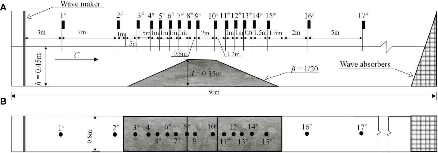
Figure 1 Experiment layout. (A) cross-section view; (B) plane view.

To ensure the two-dimensional condition wave field, the flume is divided into two parts longitudinally with widths of 0.8 m and 2.2 m by a steel wall, and the part with a width of 0.8 m is selected as the working section. The wavemaker and the absorbing device are arranged at both ends of the flume, respectively. In the experiment, the average position of the wave paddle is set to 0.0 m, and the propagation direction of waves denoted by the capital letter C is marked in Figure 1A. Wave gauges are installed at 17 different locations, the data collected by the first wave gauge which is located 3.0 m away from the zero-point location is used to obtain the initial parameters, the installation locations of other wave gauges are sketched in Figure 1. Prior experiments have shown that the reflection factor is less than 5%, therefore, the reflection effect in the present study is ignored.

In the present study, a set of irregular waves are generated based on the JONSWAP spectrum (Goda, 1999) with variable significant wave heights H_s and peak periods T_p, the peak enhancement factor is 3.3. In the experiment, the sample frequency f_s is 100 Hz, and the time duration T is 200 s. To conduct statistical analysis better, twenty realizations with different random phases for each initial spectrum are generated. Therefore, 140 data realizations are obtained. In addition, a time of about 15 minutes is needed to guarantee a still water surface between two realizations. Four peak periods are used in the tests, then the value of k_ph ranges from 1 to 3, which satisfies the finite water depth condition. Table 1 presents the details of the conditions for experimental cases. In which, f_p is the peak frequency; k_p corresponds to the wavenumber for f_p and H_max is the maximal wave height.

TABLE 1

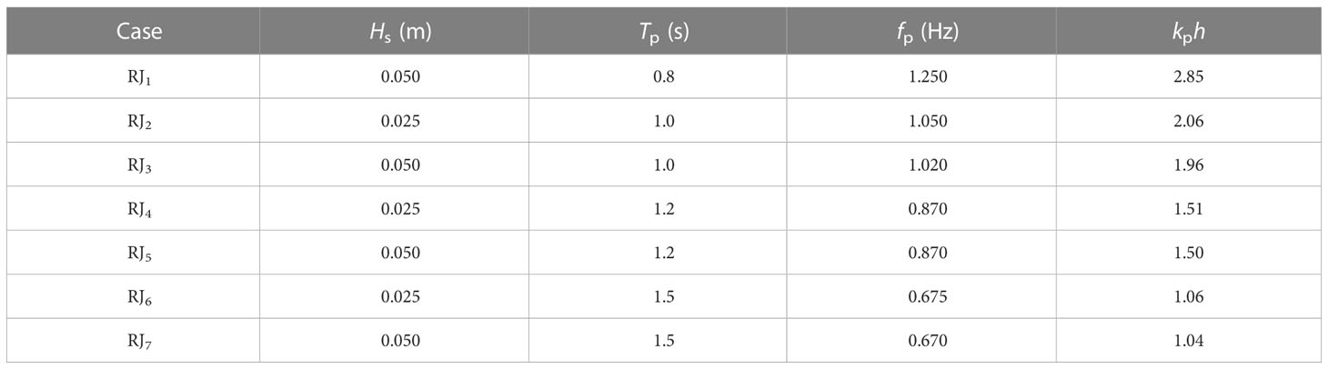
Table 1 Experimental parameters for the tests.

Results

Evolutions of wave parameters over the smooth breakwater

Water depth has a significant effect on the wave profile, Figure 2 presents the evolutions of the wave surface elevations of case RJ₇. When the wave propagates from the 0.45-m water depth to the 0.15-m water depth, sharper crests and flatter troughs make the wave profiles asymmetric. The main reasons for the transformation of the wave surface elevation are the nonlinear interactions as waves evolve over the shoaling bottom. It can be seen that the deeply asymmetric wave shapes still sustain after waves break, including the region of the whole top crest of the breakwater. When waves propagate to the de-shoaling region, the water depth increases gradually, and more symmetric wave profiles can be observed (Figure 2H). Comparing the wave profiles of the time series in the same water depths but for shoaling and de-shoaling regions, respectively, it can be seen that when waves evolve close to the top crest of the breakwater, more asymmetric wave shapes and larger crests in Figure 2D than that in Figure 2H are found. The main reason for the difference in the time series results from the quadratic nonlinear interaction and wave breaking induced by the water depth, which also affects significantly the other parameters for water waves.

FIGURE 2

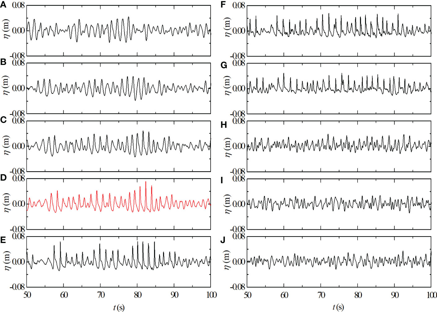
Figure 2 Wave surface elevations for case RJ₇ with T_p = 1.5 s, H_s = 0.05 m at stations: (A) 2^#; (B) 4^#; (C) 6^#; (D) 7^#; (E) 8^#; (F) 9^#; (G) 10^#; (H) 11^#; (I) 14^#and (J) 17^#. The red line denotes that wave breaking occurs at this measured location.

The nonlinear interactions are affected significantly by the topography for waves with different wavelengths and periods, the Ursell number, U_r, is always used to denote the nonlinearity and varies with the bathymetry. In the present study, the definition of Ursell Number is defined the same as (Osborne and Petti, 1994)

$\begin{array}{ll}{U}_{\text{r}}=\frac{L^2{H}_{\text{s}}}{h^3}& (15)\end{array}$

where L is the wavelength based on the mean period.

Figure 3 presents the relationship between the maximum Ursell number U_rmax, and the maximum crest height η_m, the dashed lines in the figure are the fitting curves, and the fitted equations are marked in the figure. As shown in Figure 3A, for the cases with different significant wave heights, the maximum crest heights are dependent on the maximum Ursell number linearly, in the meanwhile, the slopes for the growth curves are very close. This illustrates that the maximum Ursell numbers can well reflect the variations of the maximum crest heights with water depth.

FIGURE 3

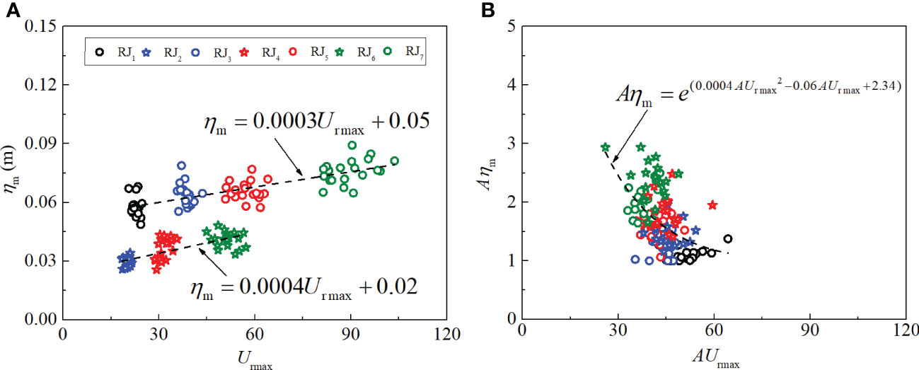
Figure 3 Scatters for the relationship between the maximum Ursell number, U_rmax, and the maximum crest height, η_m (A), and the dependence between the enlargement factors AU_rmax and Aη_m for the U_rmax and the η_m (B).

Figure 3B describes the relationship between the amplification factors AU_rmax and Aη_m. The amplification factor AU_rmax can be obtained by the maximum Ursell number along the path dividing the one at the initial position; and the amplification factor Aη_m can be obtained by the maximum crest height along the path dividing the one at the initial position. It can be seen from Figure 3B that there is an exponential dependence between the two parameters, as the maximum U_r amplifies gradually, the enlargement of the maximum crest height weakens. The declined dependence for the two expansion factors indicates that the amplification proportion for the maximum crest heights is smaller than that of the maximum Ursell number. This phenomenon reflects that the maximum Ursell number still increases rapidly when the crest height grows moderately, which indicates that when the Ursell number has a large increase with the variable topography, the crest height may grow a little. It is shown that when the wave with a longer wavelength propagates over a shallower water depth, the Ursell number may become bigger according to the equation (15), but the crest height may not grow significantly in the case of weak nonlinearity.

For the given imposed spectrum, the evolutions of the mean significant wave heights are shown in Figure 4. It can be seen that the significant wave heights increase up to the maximum as waves approach close to or on the top crest of the breakwater, and then start to decline sharply. After waves propagate across the de-shoaling region, the significant wave heights are nearly the same for cases with different wave periods in Figure 4B except for the case RJ₁ whose wave period is 0.8 s. And for this case, a continuing downward trend is found as waves evolve along the wave flume. In the present experiment, the k_ph for the case RJ₁ is about 3, and that for the others ranges from 1 to 2 (Table 1). The spatial variations of the significant wave heights illustrate that the increasing nonlinear interactions attribute to more growth of the significant wave height for cases with longer wavelengths than that for cases with shorter wavelengths. When the wavelength is longer and the water depth is smaller, the triad wave interactions and bound wave interactions increase, and the growing nonlinearity makes the peaks of the significant wave heights.

FIGURE 4

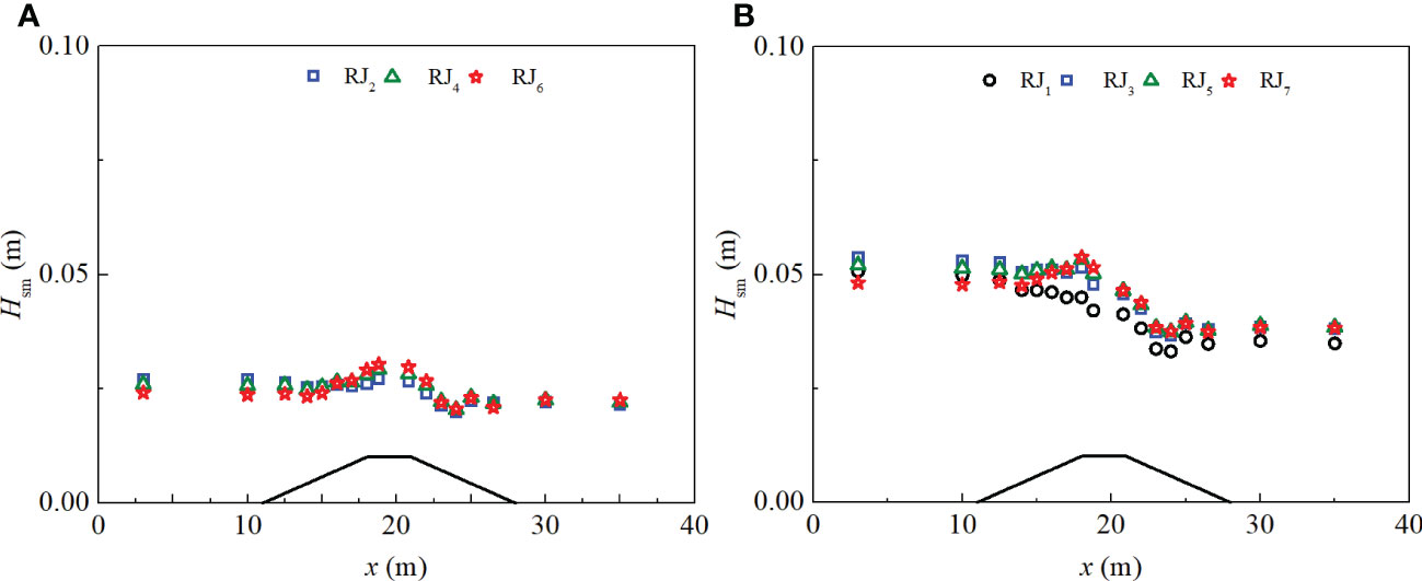
Figure 4 The evolutions of the mean significant wave heights for cases (A) with H_s = 0.025 m and (B) with H_s = 0.05 m.

Figure 5 presents the spatial variations of the mean periods, T_m, which is the mean value of the periods for all waves in a time series. It is shown that waves with longer periods are affected more obviously by uneven bathymetry. For waves with longer periods, there are two growing trends, both in the shoaling and the de-shoaling regions, respectively. The local changes in wave parameters are dependent on the nonlinear dynamic interactions induced by the variable water depths (Zhang and Benoit, 2021). This phenomenon exhibits that the transition variations of the water depth contribute to the local growth in wavelength.

FIGURE 5

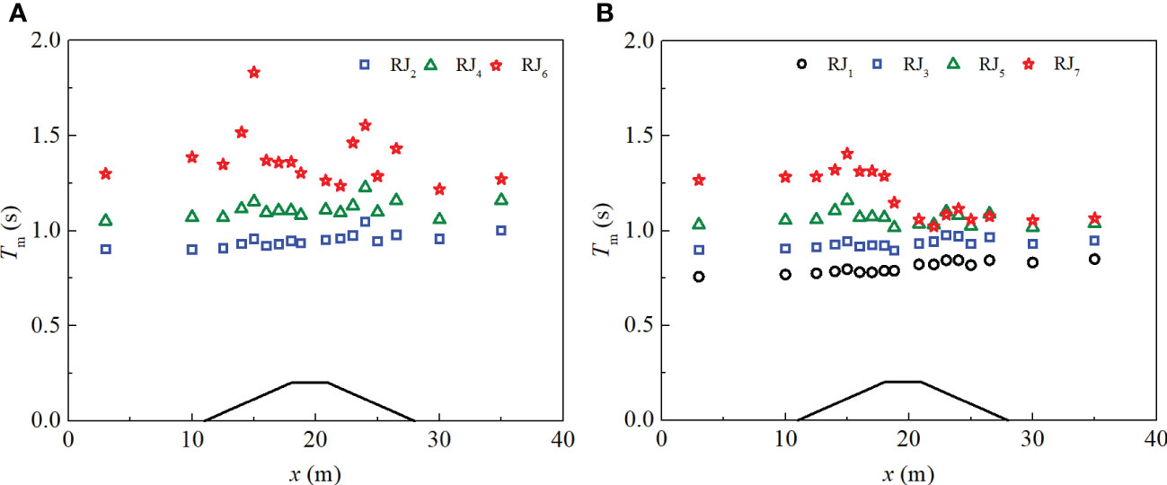
Figure 5 The evolutions of the average value for the mean period, T_m, for cases (A) with H_s = 0.025 m and (B) with H_s = 0.05 m.

Nonlinearity leads to a departure of the wave field from the Gaussian distribution (Annenkov and Shrira, 2014), which is demonstrated by the higher moments of the wave field, such as skewness and kurtosis, the analyzed results for the two parameters are shown in Figures 6, 7. When waves evolve close to and on the top crest of the breakwater, the mean kurtosis and the mean skewness can achieve their local maxima, the result is the same as that of Ma et al. (2014) and Trulsen et al. (2020). In Chen et al. (2018a)‘s study, three slopes (1/15, 1/30, and 1/45) are considered, and the value of the skewness ranges from 0 to about 1.5. The maximum skewness at a slope of 1/20 in the present study is close to that of Chen et al. (2018a). In addition, there are the minima around the end edge of the up-slope and the maxima around the start edge of the down-slope for the mean asymmetry, respectively. The results indicate that the wave profiles exhibit more asymmetric characteristics when the water depth is smaller and/or waves evolve across an abrupt transition of water depth.

FIGURE 6

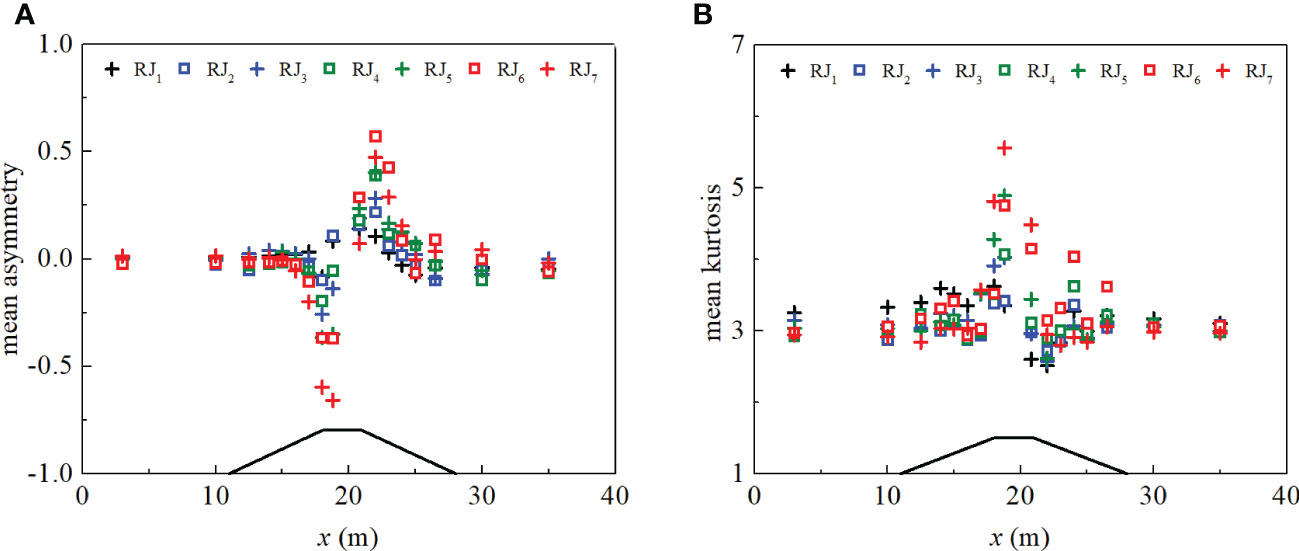
Figure 6 The evolutions of the mean asymmetry (A) and kurtosis (B).

FIGURE 7

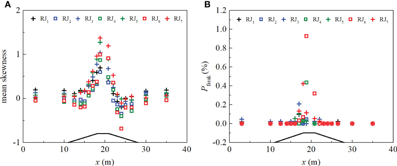
Figure 7 The evolutions for the mean skewness (A) and the probability of occurrence for the freak waves (B).

For the mean kurtosis, it looks like there is a local minimum around the shallowest part of the lee side of the breakwater at x = 22 m (11^#) as shown in Figure 6B, which is different from that of Trulsen et al. (2020). The main reason is that the kurtosis and skewness exhibit a squared dependence (Mori and Kobayashi, 1998; Ma et al., 2014), when the skewness is positive, the kurtosis grow absolutely by the skewness; however, when the skewness is negative, the kurtosis still keeps positive. In the present study, the mean skewness is negative at x = 24 m (13^#), in the meanwhile, a maximum for the mean kurtosis appears, therefore, a local minimum appears between the two local maxima shown at x = 18.8 m (9^#) and x = 24 m (13^#), respectively. In addition, in Trulsen et al. (2020), the slope rate for the up-slope is 0.263 and the parameter is 0.05 for this region in the present study. The transition variation in this experiment is milder than that of Trulsen et al. (2020); correspondingly, the nonlinear increases slower. For the 140 realizations, all the freak waves are detected. In Figure 7B, it can be seen that the probability of freak wave occurrence is the highest when the mean kurtosis and the mean skewness achieve the maxima, as waves propagate close to the top crest of the breakwater, the maximum probability of occurrence for the freak wave can be up to about 1%.

Figure 8 exhibits the maximum crest heights and wave heights for the freak waves. It is shown that the maximum crest heights and wave heights for cases with H_s = 0.025 m change mildly and they fluctuate around the values of 0.04 m and 0.06 m, respectively as shown in Figure 8A. However, they vary significantly for the cases with the H_s = 0.05 m, as shown in Figure 8B. The crest heights fluctuate between 0.04 m - 0.08 m, and the wave heights fluctuate between 0.055 m - 0.12 m. The comparison above illustrates that the significant wave height has an important effect on the local maximum crest heights and the maximum wave heights of the freak waves.

FIGURE 8

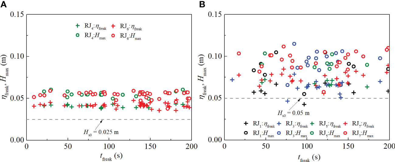
Figure 8 The crest heights of the freak waves and the maximum wave heights for cases (A) with H_s = 0.025 m and (B) with H_s = 0.05 m, t_freak is the occurrence time of the freak wave.

Following Figures 8, 9 shows the ratio, R, between the crest heights of the freak waves and the maximum wave heights. The results show that the values of R for cases with different significant wave heights fluctuate around a similar level, 0.7. It can indicate that the mean ratio between the crest height and the maximum wave height is close to a constant for the freak waves. It is noted that the definition of the ratio R is the same as the horizontal asymmetry factor shown in Bonmarin (1989) if the maximum wave height is the one containing the maximum crest height and is defined by zero-downcross analysis. In their study, the mean horizontal asymmetry factor ranges from 0.69 - 0.77 for variable breaking types that occurred in deep water. It can be seen that the mean ratio R for the freak wave in finite water depth is within the scale of the mean horizontal asymmetry factor for breaking waves in deep water.

FIGURE 9

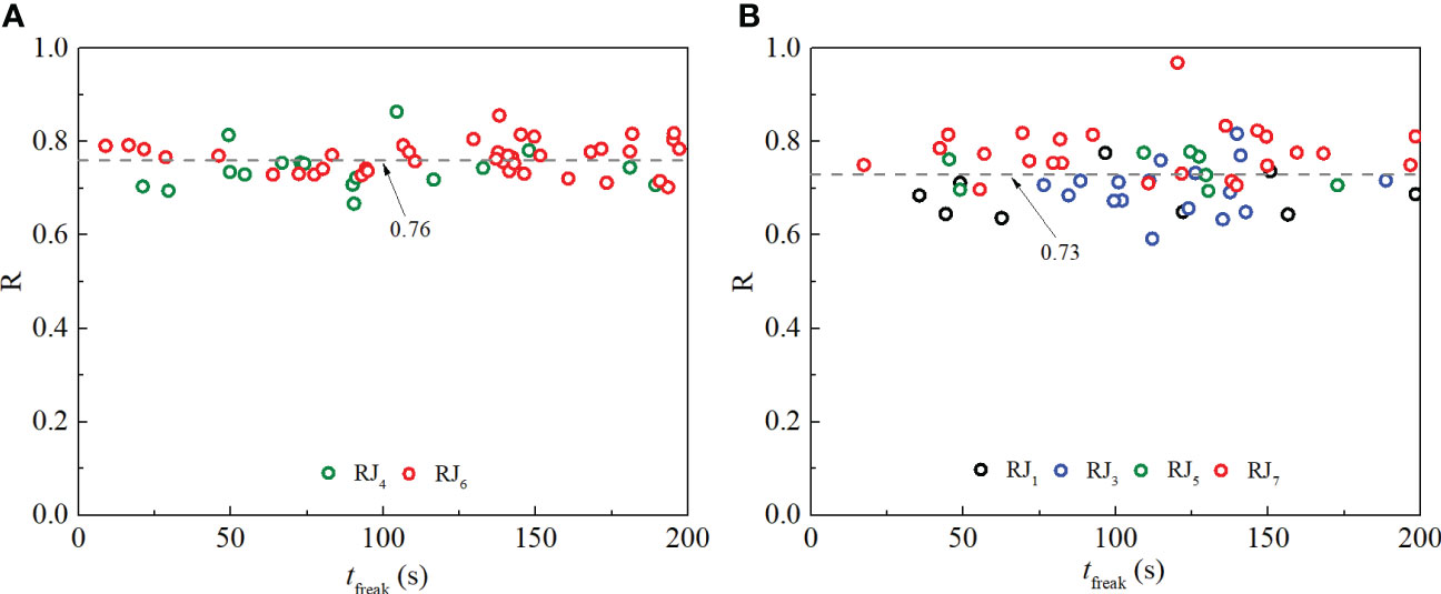
Figure 9 The ratio between the crest heights of the freak waves and the maximum wave heights for cases (A) with H_s = 0.025 m and (B) with H_s = 0.05 m, t_freak is the occurrence time of the freak wave, the values of 0.76 and 0.73 are the average value for cases in (A, B), respectively.

Transformation of spectra over the smooth breakwater

From the analysis above, it can be seen that the increasing nonlinearity makes the wave parameters change a lot (Figures 2, 6, 7), especially for the freak waves. In this section, the nonlinear interactions coupling their evolution of the wave over uneven bathymetry are studied in terms of spectra. The information on the frequency modulation can reflect nonlinearity well (Wu and Yao, 2004; Veltcheva and Soares, 2016). Taking the case RJ₇ as an example, the freak wave occurs at the location of x = 17 m (7^#), and the evolutions of the Hilbert spectra and the wavelet-based bicoherences are presented in Figures 10, 11. In Figure 10A, the spectrum presents that the energy of waves mainly resides in the dominant frequency when the water depth is 0.45 m. Referring to Figure 11A, it also can be seen that the interaction between waves is weak. As the wave evolves along the up-slope, water depth decreases, and the frequency modulation actions appear apparently in Figures 10C, D, especially the latter. It can be found that the frequency modulation can increase up to about 4 Hz at 80 s around when the freak wave occurs.

FIGURE 10

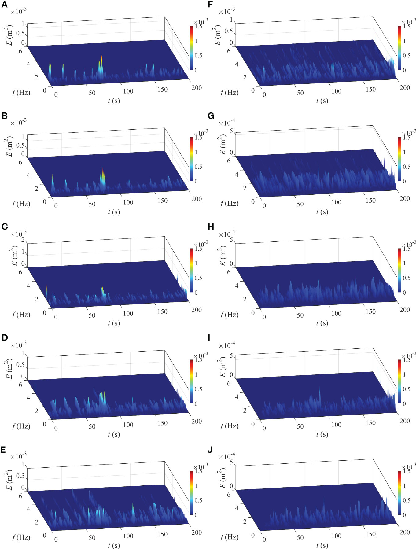
Figure 10 Evolutions of the three-dimensional Hilbert spectra for the case RJ₇ at stations: (A) 2^#; (B) 4^#; (C) 6^#; (D) 7^#; (E) 8^#; (F) 9^#; (G) 10^#; (H) 11^#; (I) 14^# and (J) 17^#; the freak wave occurs at station 7^#.

FIGURE 11

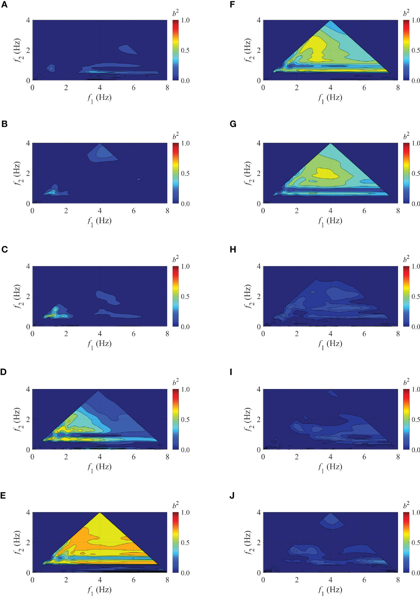
Figure 11 Evolutions of the wavelet-based bicoherence for the case RJ₇ at stations: (A) 2^#; (B) 4^#; (C) 6^#; (D) 7^#; (E) 8^#; (F) 9^#; (G) 10^#; (H) 11^#; (I) 14^# and (J) 17^#; the freak wave occurs at station 7^#.

Corresponding to the increasing frequency modulation, the interactions between waves grow significantly in Figures 11C, D. Comparison of Figures 10C, 11C, as the wave depth decreases, the interactions between primary waves, and that between the primary waves and the high-order harmonics start to grow; it can be reflected by b² (0.66, 0.66) = 0.27 and b² (1.32, 0.66) = 0.42. The variations in bicoherence illustrate that the nonlinear phase coupling between modes becomes obvious and the energy is transferred to 1.32 Hz and 1.98 Hz with the decreasing water depth. Accordingly, Figure 10C shows the same tendency at t = 10 s, 30 s, and 80 s around. When the water depth is reduced to 0.15 m, the Hilbert spectrum and wavelet-based bicoherence are shown in Figures 10D, 11D, respectively. The active nonlinear interactions can be found, and the number of wave modes involved in quadratic phase coupling increases obviously. Figure 11D shows that the energy is transferred to the high-frequency contents significantly as the water depth decreases, for example, b² (1.32, 0.66) = 0.56, b² (2.64, 0.66) = 0.61, b² (3.3, 0.66) = 0.64, b² (2.64, 1.32) = 0.6, b² (1.14, 0.74) = 0.72, b² (1.98, 0.66) = 0.68, b² (1.98, 1.32) = 0.62 and b² (2.16, 1.84) = 0.61, they are consistent with the energy growth at f = 1.98 Hz, f = 3.3 Hz, f = 3.96 Hz, f = 3.96 Hz, f = 1.88 Hz, f = 2.64 Hz, f = 3.3 Hz, and f = 4 Hz. Referring to Figure 10D, it can be seen that the frequency modulation acts strongly, especially, at t = 80 s around, 4 Hz component gains obvious energy, which can reflect the occurrence time for the triad wave interactions, corresponding to the components f₁ = 2.16 Hz, f₂ = 1.84 Hz, and f = 4 Hz.

When the wave moves to the top peak of the bar, the water depth is 0.1 m and the wave breaks. Figure 10E shows that more energy is transferred to the high-frequency components; especially, there’s even significant energy transferred to 5 Hz components. The substantial energy that appeared in high-frequency contents is mainly derived from the frequency modulation between wave components. Referring to Figure 11E, when the wave propagates in a depth of 0.1 m, the three-wave interactions appear more prominently, and many wave modes are involved in the nonlinear phase coupling, such as b² (0.66, 0.66) = 0.45, b² (1.32, 0.66) = 0.61, b² (2.64, 0.66) = 0.71, b² (3.3, 0.66) = 0.74, b² (1.98, 0.66) = 0.65, b² (1.98, 1.32) = 0.61, b² (2.64, 1.32) = 0.67, b² (1.14, 0.74) = 0.67, and b² (2.16, 1.84) = 0.75. By comparing the analysis results at 0.15 m water depth, it can be seen that the energy residing in components with 1.32, 1.98, 3.3, 3.96, and 4 Hz keeps increasing, which derives mainly from the interactions between the primary waves, the primary waves and their high-order harmonics, and the extent of the phase coupling is strong. However, there are also energy reductions in some components, such as 2.64, 3.3, and 1.88 Hz by tracing the decrease of b² (1.98, 0.66), b² (1.98, 1.32) and b² (1.14, 0.74), which illustrates that the quadratic phase coupling relationship between components with 1.98 and 0.66 Hz, 1.98 and 1.32 Hz and 1.14 and 0.74 Hz diminishes. It needs to be noted that the energy residing in the component with 3.3 Hz not only increases but decreases at this location, the quadratic phase coupling relationship between components with 2.64 and 0.66 Hz grows and transfers energy to 3.3 Hz; while the nonlinear quadratic phase coupling relationship between components with 1.98 and 1.32 Hz weakens. Referring to Figure 10E, the quadratic phase coupling mainly occurs before 100 s. At the whole top peak of the bar, Figures 10E–G shows that the frequency modulation acts significantly, and the energy of the high-frequency components increases substantially. The significant variations also are exhibited in Figures 11E–G.

In the de-shoaling region (Figures 10H–J), an obvious reduction in frequency modulation is shown, the energy of all wave components is concentrated below 2 Hz, compared with Figures 10A–C, the energy distribution in this region is more uniform with time. The obvious changes are also exhibited in Figures 11H–J, the evolutions of the squared bicoherence spectra indicate that the range of the wave modes which are involved in the nonlinear phase coupling is reduced.

According to the above analysis, the frequency modulation is closely related to the nonlinear quadratic phase coupling as the water depth varies. When the water depth decreases, the quadratic nonlinear interactions strengthen, and the frequency modulation acts strongly. However, when the water depth increases, the quadratic nonlinear phase coupling and the frequency modulation decrease simultaneously.

For the same case, the difference between the energy spectra by FFT at locations x = 17 m (7^#) and x = 10 m (2^#) is described in Figure 12 to investigate the energy transformation in the process of the wave growing into a freak wave. There is an obvious increase in the low- and high-frequency contents, this also can be found in Figures 10, 11, this growth is mainly induced by the triad wave interactions as waves evolve over the shallower water depth.

FIGURE 12

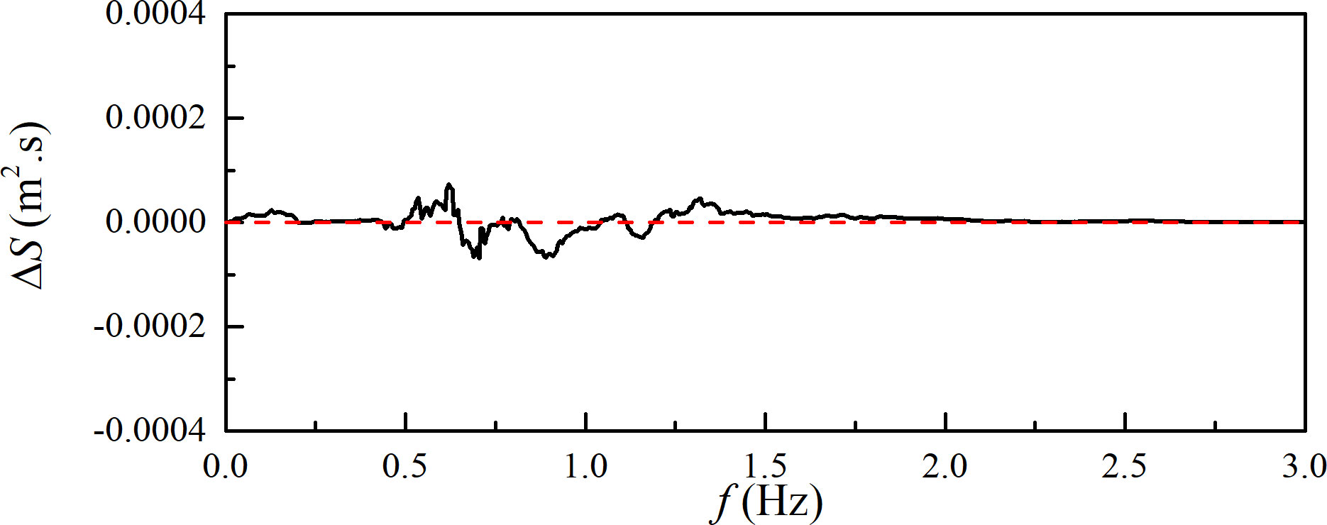
Figure 12 The difference of spectra between the stations 7^# and 2^# for case RJ₇.

After the extreme event, wave breaking occurs, and the difference between the spectra at the locations x = 18 m (8^#) and x = 17 m (7^#) is presented in Figure 13. It can be seen that the energy in the region of the dominant frequency is dissipated a lot after the wave breaking, and the high-frequency energy still increases. The energy variation illustrates that as the wave propagates over the depth of water getting shallower, the triad wave interactions increase, and the energy of the bound waves derived from the sum and the difference of the intrinsic frequencies grows. And when waves evolve coupling with the breaker, the energy of the dominant frequency band is dissipated, in the meanwhile, some bound waves are released to be free waves, these free waves may take part in the triad wave interactions as the water depth continues to decline. The increased energy in high-frequency contents can be referred to in Figures 10E, 11E.

FIGURE 13

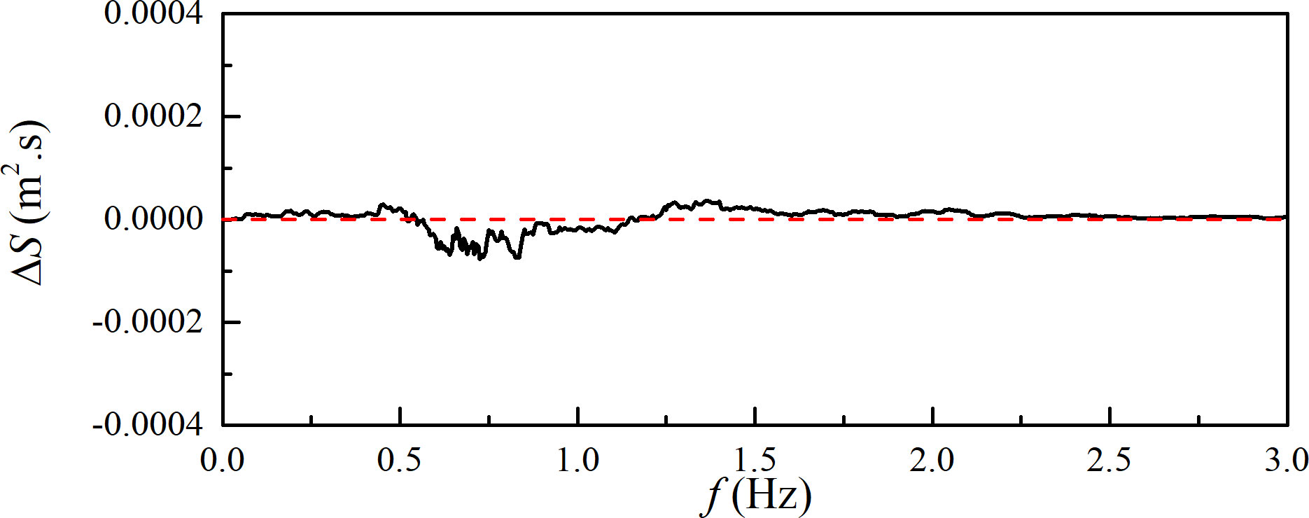
Figure 13 The difference of spectra between the stations 8^# and 7^# for case RJ₇.

When waves evolve on the top peak of the breakwater, the difference between the spectra at the locations x = 20.8 m (10^#) and x = 18 m (8^#) is presented in Figure 14. Energy in the regions of the dominant and low frequencies dissipates sharply, and that in the region of the high frequency still increases. The obvious decrease in energy of the dominant-frequency region may be induced by many small wave breaking. The increase in energy of the high-frequency contents can be found in Figures 10E, G, 11E–G). The triad wave interactions and the frequency modulation are all significant when waves evolve on the top of the breakwater, which indicates that the triad wave interactions depend on the frequency modulation. In the meanwhile, the high-frequency free waves maybe also a factor contributing to the increase of high-frequency energy.

FIGURE 14

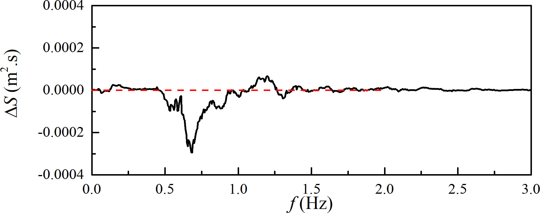
Figure 14 The difference of spectra between the stations 10^# and 8^# for case RJ₇.

Discussion and conclusion

In the present study, the nonlinear characteristics of the irregular random waves propagating over the uneven bathymetry are discussed. The effects of the varying water depths on the nonlinear interactions are investigated in terms of the wave surface evolutions, geometric parameters, and energy spectra. The shoal effect contributes to the sharp crests and the flat troughs. A value of about 0.7 of the ratio between the maximum crest heights and the maximum wave heights of the wave profiles for the freak waves is found, which illustrates that there is a local intense energy focus on the crest for the freak wave, therefore the extreme event will appear.

As waves evolve with the decreasing water depth, the nonlinear phase coupling increases by the bicoherence spectrum, and significant energy is transferred to high-frequency contents in terms of obvious frequency modulation. After wave breaking occurs, the energy of the dominant-frequency region is dissipated (ignoring the viscous and friction loss) and the energy in the high-frequency region is increased. By analyzing the variations of the nonlinear interactions as the wave evolves over the variable-depth bathymetry, the results show that the frequency modulation can reflect the triad wave interactions very well, and the abrupt increase in the frequency modulation can indicate the appearance of the extreme event.

In the present investigation, even though the nonlinear characteristics of geometric parameters, three-wave interactions, and frequency modulation are studied and some meaningful results are obtained here, some contents need to be learned further due to the limited conditions. More peak factors of the JONSWAP spectrum need to be considered for expanding the scope of the study. The essential relationship between the frequency modulation and the nonlinear phase coupling interaction in shallow water is still not revealed, therefore, more wave conditions are essential to study further to find more characteristics associated with them.

Data availability statement

The raw data supporting the conclusions of this article will be made available by the authors, without undue reservation.

Author contributions

YH contributed to the data analysis and the paper writing. GW improved the grammar of the manuscript. HM improved the words. HC designed and conducted the experiment. JL reviewed the manuscript. GD provided the equipment and conditions for the experiment. All authors contributed to the article and approved the submitted version.

Funding

This work was financially supported by the Ocean Youth Talent Project of Zhanjiang Science and Technology Bureau [grant number 2021E05010]; the Doctor Initiate Projects of Guangdong Ocean University [grant number 120602-R20069]; the National Natural Science Foundation of China [grant number 52001071]; the Special fund competition allocation project of Guangdong Science and Technology Department [grant number 2021A05227]; and the Youth Innovative Talent Project of the Guangdong Education Bureau [grant number 2019KQNCX045].

Acknowledgments

The authors would like to express their sincere thanks to Yuxiang Ma and Xiaozhou Ma who have offered support.

Conflict of interest

The authors declare that the research was conducted in the absence of any commercial or financial relationships that could be construed as a potential conflict of interest.

Publisher’s note

All claims expressed in this article are solely those of the authors and do not necessarily represent those of their affiliated organizations, or those of the publisher, the editors and the reviewers. Any product that may be evaluated in this article, or claim that may be made by its manufacturer, is not guaranteed or endorsed by the publisher.

References

Annenkov S. Y., Shrira V. I. (2014). Evaluation of skewness and kurtosis of wind waves parameterized by JONSWAP spectra. J. Phys. Oceanogr 44 (6), 1582–1594. doi: 10.1175/jpo-d-13-0218.1

CrossRef Full Text | Google Scholar

Baldock T. E., Swan C. (1996). Extreme waves in shallow and intermediate water depths. Coast. Eng. 27, 21–46. doi: 10.1016/0378-3839(95)00040-2

CrossRef Full Text | Google Scholar

Beji S., Battjes J. A. (1993). Experimental investigation of wave propagation over a bar. Coast. Eng. 19, 151–162. doi: 10.1016/0378-3839(93)90022-Z

CrossRef Full Text | Google Scholar

Bonmarin P. (1989). Geometric properties of deep-water breaking waves. J. Fluid Mechanics 209 (1), 405–433. doi: 10.1017/s0022112089003162

CrossRef Full Text | Google Scholar

Chen H. Z., Tang X. C., Gao J. L., Fan G. X. (2018a). Parameterization of geometric characteristics for extreme waves in shallow water. Ocean Eng. 156, 61–71. doi: 10.1016/j.oceaneng.2018.02.067

CrossRef Full Text | Google Scholar

Chen H. Z., Tang X. C., Zhang R., Gao J. L. (2018b). Effect of bottom slope on the nonlinear triad interactions in shallow water. Ocean Dynamics 68 (4-5), 469–483. doi: 10.1007/s10236-018-1143-y

CrossRef Full Text | Google Scholar

Cherneva Z., Soares C. G. (2007). Estimation of the bispectra and phase distribution of storm sea states with abnormal waves. Ocean Eng. 34 (14-15), 2009–2020. doi: 10.1016/j.oceaneng.2007.02.010

CrossRef Full Text | Google Scholar

Christou M., Swan C., Gudmestad O. T. (2008). The interaction of surface water waves with submerged breakwaters. Coast. Eng. 55 (12), 945–958. doi: 10.1016/j.coastaleng.2008.02.014

CrossRef Full Text | Google Scholar

Crawford A. M., Hay A. E. (2003). Wave orbital velocity skewness and linear transition ripple migration: Comparison with weakly nonlinear theory. J. Geophys Res. 108 (C3), 36–(1–6). doi: 10.1029/2001jc001254

CrossRef Full Text | Google Scholar

Doering J. C., Bowen A. J. (1995). Parametrization of orbital velocity asymmetries of shoaling and breaking waves using bispectral analysis. Coast. Eng. 26, 15–33. doi: 10.1016/0378-3839(95)00007-X

CrossRef Full Text | Google Scholar

Dong G. H., Chen H. Z., Ma Y. X. (2014). Parameterization of nonlinear shallow water waves over sloping bottoms. Coast. Eng. 94, 23–32. doi: 10.1016/j.coastaleng.2014.08.012

CrossRef Full Text | Google Scholar

Dong G. H., Ma Y. X., Ma X. Z., Perlin M., Yu B., Xu J. W. (2008). Experimental study of wave-wave nonlinear interactions using the wavelet-based bicoherence. Coast. Eng. 55 (9), 741–752. doi: 10.1016/j.coastaleng.2008.02.015

CrossRef Full Text | Google Scholar

Dysthe K., Krogstad H. E., Müller P. (2008). Oceanic rogue waves. Annu. Rev. Fluid Mechanics 40 (1), 287–310. doi: 10.1146/annurev.fluid.40.111406.102203

CrossRef Full Text | Google Scholar

Elgar S., Guza R. T. (1985). Observations of bispectra of shoaling surface gravity waves. J. Fluid Mechanics 161, 425–448. doi: 10.1017/S0022112085003007

CrossRef Full Text | Google Scholar

Fu R. L., Ma Y. X., Dong G. H., Perlin M. (2021). A wavelet-based wave group detector and predictor of extreme events over unidirectional sloping bathymetry. Ocean Eng. 229, 108936. doi: 10.1016/j.oceaneng.2021.108936

CrossRef Full Text | Google Scholar

Gao J. L., Ma X. Z., Zang J., Dong G. H., Ma X. J., Zhu Y. Z., et al. (2020). Numerical investigation of harbor oscillations induced by focused transient wave groups. Coast. Eng. 158, 103670. doi: 10.1016/j.coastaleng.2020.103670

CrossRef Full Text | Google Scholar

Goda Y. (1999). A comparative review on the functional forms of directional wave spectrum. Coast. Eng. J. 41 (1), 1–20. doi: 10.1142/S0578563499000024

CrossRef Full Text | Google Scholar

Gramstad O., Zeng H., Trulsen K., Pedersen G. K. (2013). Freak waves in weakly nonlinear unidirectional wave trains over a sloping bottom in shallow water. Phys. Fluids 25 (12), 122103–(1–14). doi: 10.1063/1.4847035

CrossRef Full Text | Google Scholar

He Y. L., Ma Y. X., Mao H. F., Dong G. H., Ma X. Z. (2022). Predicting the breaking onset of wave groups in finite water depths based on the Hilbert-Huang transform method. Ocean Eng. 247, 110733. doi: 10.1016/j.oceaneng.2022.110733

CrossRef Full Text | Google Scholar

Huang N. E., Shen Z., Long S. R., Wu M. C., Shih H. H., Zheng Q., et al. (1998). The empirical mode decomposition and the Hilbert spectrum for nonlinear and non-stationary time series analysis. Proc. R. Soc. A: Mathematical Phys. Eng. Sci. 454 (1971), 903–995. doi: 10.1098/rspa.1998.0193

CrossRef Full Text | Google Scholar

Kharif C., Pelinovsky E. (2003). Physical mechanisms of the rogue wave phenomenon. Eur. J. Mechanics - B/Fluids 22 (6), 603–634. doi: 10.1016/j.euromechflu.2003.09.002

CrossRef Full Text | Google Scholar

Li J. X., Yang J. Q., Liu S. X., Ji X. R. (2015). Wave groupiness analysis of the process of 2D freak wave generation in random wave trains. Ocean Eng. 104, 480–488. doi: 10.1016/j.oceaneng.2015.05.034

CrossRef Full Text | Google Scholar

Ma Y. X., Chen H. Z., Ma X. Z., Dong G. H. (2017). A numerical investigation on nonlinear transformation of obliquely incident random waves on plane sloping bottoms. Coast. Eng. 130, 65–84. doi: 10.1016/j.coastaleng.2017.10.003

CrossRef Full Text | Google Scholar

Ma Y. X., Dong G. H., Ma X. Z. (2014). Experimental study of statistics of random waves propagating over a bar. Coast. Eng. Proc. 1 (34), 30. doi: 10.9753/icce.v34.waves.30

CrossRef Full Text | Google Scholar

Ma Y. X., Ma X. Z., Perlin M., Dong G. H. (2013). Extreme waves generated by modulational instability on adverse currents. Phys. Fluids 25 (11), 114109. doi: 10.1063/1.4832715

CrossRef Full Text | Google Scholar

Mahmoudof S. M., Badiei P., Siadatmousavi S. M., Chegini V. (2016). Observing and estimating of intensive triad interaction occurrence in very shallow water. Continental Shelf Res. 122, 68–76. doi: 10.1016/j.csr.2016.04.003

CrossRef Full Text | Google Scholar

Mahmoudof S. M., Hajivalie F. (2021). Experimental study of hydraulic response of smooth submerged breakwaters to irregular waves. Oceanologia 63 (4), 448–462. doi: 10.1016/j.oceano.2021.05.002

CrossRef Full Text | Google Scholar

Mori N., Kobayashi N. (1998). Nonlinear distribution of neashore free surface and velocity. Coast. Eng. 1, 189–202. doi: 10.1061/9780784404119.013

CrossRef Full Text | Google Scholar

Osborne A. R., Petti M. (1994). Laboratory-generated, shallow-water surface waves: Analysis using the periodic, inverse scattering transform. Phys. Fluids 6 (5), 1727–1744. doi: 10.1063/1.868235

CrossRef Full Text | Google Scholar

Pelinovsky E., Sergeeva A. (2006). Numerical modeling of the KdV random wave field. Eur. J. Mechanics - B/Fluids 25 (4), 425–434. doi: 10.1016/j.euromechflu.2005.11.001

CrossRef Full Text | Google Scholar

Peng Z., Zou Q., Reeve D., Wang B. (2009). Parameterisation and transformation of wave asymmetries over a low-crested breakwater. Coast. Eng. 56 (11-12), 1123–1132. doi: 10.1016/j.coastaleng.2009.08.005

CrossRef Full Text | Google Scholar

Sergeeva A., Pelinovsky E., Talipova T. (2011). Nonlinear random wave field in shallow water: variable korteweg-de Vries framework. Natural Hazards Earth System Sci. 11 (2), 323–330. doi: 10.5194/nhess-11-323-2011

CrossRef Full Text | Google Scholar

Shukla P. K., Kourakis I., Eliasson B., Marklund M., Stenflo L. (2006). Instability and evolution of nonlinearly interacting water waves. Phys. Rev. Lett. 97 (9), 94501. doi: 10.1103/PhysRevLett.97.094501

CrossRef Full Text | Google Scholar

Teng B., Ning D. Z. (2009). A simplified model for extreme-wave kinematics in deep sea. J. Mar. Sci. Appl. 8 (1), 27–32. doi: 10.1007/s11804-009-8046-8

CrossRef Full Text | Google Scholar

Trulsen K., Raustøl A., Jorde S., Rye L. (2020). Extreme wave statistics of long-crested irregular waves over a shoal. J. Fluid Mechanics 882, R2. doi: 10.1017/jfm.2019.861

CrossRef Full Text | Google Scholar

Trulsen K., Zeng H., Gramstad O. (2012). Laboratory evidence of freak waves provoked by non-uniform bathymetry. Phys. Fluids 24 (9), 740–310. doi: 10.1063/1.4748346

CrossRef Full Text | Google Scholar

Veltcheva A. D. (2001). “Wave groupiness in the nearshore area by hilbert spectrum,” in Fourth international symposium on ocean wave measurement and analysis (San Francisco, California, United States: American Society of Civil Engineers).

Google Scholar

Veltcheva A., Soares C. G. (2016). Nonlinearity of abnormal waves by the Hilbert–Huang transform method. Ocean Eng. 115, 30–38. doi: 10.1016/j.oceaneng.2016.01.031

CrossRef Full Text | Google Scholar

Whittaker C. N., Raby A. C., Fitzgerald C. J., Taylor P. H. (2016). The average shape of large waves in the coastal zone. Coast. Eng. 114, 253–264. doi: 10.1016/j.coastaleng.2016.04.009

CrossRef Full Text | Google Scholar

Wu Z. H., Huang N. E. (2008). Ensemble empirical mode decomposition: A noise assisted data analysis method. Adv. Adaptive Data Anal. 1 (1), 1–41. doi: 10.1142/S1793536909000047

CrossRef Full Text | Google Scholar

Wu C. H., Yao A. F. (2004). Laboratory measurements of limiting freak waves on currents. J. Geophys Res. 109 (C12), C12002. doi: 10.1029/2004jc002612

CrossRef Full Text | Google Scholar

Zhang J., Benoit M. (2021). Wave–bottom interaction and extreme wave statistics due to shoaling and de-shoaling of irregular long-crested wave trains over steep seabed changes. J. Fluid Mechanics 912, A28–(1–34). doi: 10.1017/jfm.2020.1125

CrossRef Full Text | Google Scholar

Zhao X. Z., Hu C. H., Sun Z. C. (2010). Numerical simulation of extreme wave generation using VOF method. J. Hydrodynamics 22 (4), 466–477. doi: 10.1016/s1001-6058(09)60078-0

CrossRef Full Text | Google Scholar

Zou Q., Peng Z. (2011). Evolution of wave shape over a low-crested structure. Coast. Eng. 58 (6), 478–488. doi: 10.1016/j.coastaleng.2011.01.001

CrossRef Full Text | Google Scholar