
95% of researchers rate our articles as excellent or good
Learn more about the work of our research integrity team to safeguard the quality of each article we publish.
Find out more
ORIGINAL RESEARCH article
Front. Mar. Sci. , 04 April 2023
Sec. Ocean Observation
Volume 10 - 2023 | https://doi.org/10.3389/fmars.2023.1150651
This article is part of the Research Topic Deep Learning for Marine Science View all 40 articles
 Jack H. Prior1*
 Matthew D. Campbell2
 Matthew Dawkins3
 Paul F. Mickle4
 Robert J. Moorhead5
 Simegnew Y. Alaba5Chiranjibi Shah5Joseph R. Salisbury6
 Kevin R. Rademacher2
 A. Paul Felts2Farron Wallace7
Increased necessity to monitor vital fish habitat has resulted in proliferation of camera-based observation methods and advancements in camera and processing technology. Automated image analysis through computer vision algorithms has emerged as a tool for fisheries to address big data needs, reduce human intervention, lower costs, and improve timeliness. Models have been developed in this study with the goal to implement such automated image analysis for commercially important Gulf of Mexico fish species and habitats. Further, this study proposes adapting comparative otolith aging methods and metrics for gauging model performance by comparing automated counts to validation set counts in addition to traditional metrics used to gauge AI/ML model performance (such as mean average precision - mAP). To evaluate model performance we calculated percent of stations matching ground-truthed counts, ratios of false-positive/negative detections, and coefficient of variation (CV) for each species over a range of filtered outputs using model generated confidence thresholds (CTs) for each detected and classified fish. Model performance generally improved with increased annotations per species, and false-positive detections were greatly reduced with a second iteration of model training. For all species and model combinations, false-positives were easily identified and removed by increasing the CT to classify more restrictively. Issues with occluded fish images and reduced performance were most prevalent for schooling species, whereas for other species lack of training data was likely limiting. For 23 of the examined species, only 7 achieved a CV less than 25%. Thus, for most species, improvements to the training library will be needed and next steps will include a queried learning approach to bring balance to the models and focus during training. Importantly, for select species such as Red Snapper (Lutjanus campechanus) current models are sufficiently precise to begin utilization to filter videos for automated, versus fully manual processing. The adaption of the otolith aging QA/QC process for this process is a first step towards giving researchers the ability to track model performance through time, thereby giving researchers who engage with the models, raw data, and derived products confidence in analyses and resultant management decisions.
Management of fish populations requires estimates of abundance, age/length composition, fecundity, mortality, and other life history variables sampled representatively from a stock (Jennings and Kaiser, 1998). Monitoring efforts are becoming increasingly critical as populations are impacted by multiple stressors such as fishing, climate change, biotic perturbations (e.g., hypoxia), habitat loss, and rising levels of pollution (e.g., microplastics). Historically, resource surveys were conducted using a wide-variety of traditional fisheries gears such as trawls, traps, and nets. Over the past 30 to 40 years, optics-based sampling methods have become a more common practice as they avoid issues with problematic habitats such as reefs, and have fewer issues with size and species selectivity (Cappo et al., 2007). Moreover, optical sampling with BRUVs (Baited Remote Underwater Videos) is less invasive, non-lethal, and can also provide valuable habitat data valuable for single-species and ecosystem-based management (EBM) and ecosystem-based fisheries management (EBFM).
One downside associated with optical sampling is the immense amount of data collected and, in turn, the human effort required to post-process collections (i.e. annotate). For example, one year of sampling of the combined Gulf Fishery Independent Survey of Habitat and Ecosystem Resources (GFISHER) and the Southeast Area Monitoring and Assessment Reef Fish Video (SEAMAP-RFV) surveys results in ~2000 camera deployments, ~1000 hrs of video, and ~30 TB of data requiring annotation (hereafter GFISHER refers to these surveys in combination). Extrapolated across NMFS Science Centers, state agencies, academic laboratories, and non-governmental organizations, the big-data issue quickly becomes overwhelming. In response, the National Marine Fisheries Service (NMFS) funded the Automated Image Analysis Strategic Initiative (AIASI) with the goal of producing software that can be trained on object detection and classification using artificial intelligence/machine learning (AI/ML) across a wide variety of natural resources. A major outcome of the AIASI was the development of the Video and Image Analytics in the Marine Environment (VIAME ©) software in partnership with Kitware Inc. (Clifton Park, NY).
New developments in graphics processing units (GPU) technology and artificial AI/ML processes can provide a means to reduce human effort for post-processing data collected in marine habitats (van Helmond et al., 2020). Frame level count data can be generated using algorithm outputs from which any number of metrics (e.g., MaxN and MeanCount) could be estimated. Among the many advantages to applying algorithms to process data over human video readers are that processing can occur 24/7, detection and identification are standardized to a single algorithm, inter and intra-reader variability is reduced, and computing costs are relatively inexpensive, particularly when considering the efficiencies in post-processing potentially gained. Additionally, features that may be missed by human eyes can be discerned and recognized by computer vision. The GPU-based classifications remain consistent and do not change based on human moods or energy levels. Despite their burgeoning development and promise, questions pertaining to algorithm accuracy and precision remain, particularly those related to sampling conditions that might limit their reliability (e.g., water visibility). This is especially important because long-term time-series require that data annotated using AI/ML is compatible with the human annotations conducted historically. This is critical in cases for which historic video is unavailable for re-processing using AI/ML methods (e.g., non-digital formats, or lost/destroyed video).
When evaluating model performance using a subset of training imagery, AI/ML algorithms have demonstrated excellent performance in detection and classification of a wide-variety of object classes (Zion et al., 2007). Yet analysis of in situ collections show less accuracy and precision than is suggested by analyzing precision using a subset of training imagery (Salman et al., 2020). For instance, water turbidity and/or low light intensity may reduce model accuracy and precision (Marini et al., 2018). In addition, videos with increased fish density (i.e., fish/unit area) and higher levels of species diversity may be more difficult for algorithms to process accurately. Rugose habitats of reefs may lead to larger numbers of false negatives/positives in fish detections due to cryptic behavior and/or coloring and mottling that resembles complex habitat (e.g., lionfish). Fish species of different size classes and with different swimming or schooling behaviors may be harder to detect or classify than others (Lopez-Marcano et al., 2022), especially at variable distances from a camera at a fixed position (mobile cameras face their own challenges). Regardless of the source of error, the main challenge is that the annotation phase of post-processing is likely impacted by detection and identification differences arising from variable environmental conditions in which video is collected, and therefore great care has to be taken to ensure that time-series remain stable relative to changes made in post-processing methods. Put more simply, there are inevitable differences between manual and automated processing that have to be analyzed, evaluated and compensated for if necessary.
A common approach to solving the wide variety of problems associated with using AI/ML for classification and enumeration (e.g., schooling) is to use different model architectures and mathematical algorithms. For instance, convolutional neural networks (CNN) have been shown to produce higher accuracy than older methods such as Support-Vector Machine (SVM) models, Gaussian-Mixture Modeling (GMM), or You-Only-Look-Once (YOLO) based approaches (Cui et al., 2020; Marrable et al., 2022). Fish detection at the frame level has been achieved by many researchers and with relatively high levels of accuracy (Chuang et al., 2014; Villon et al., 2016; Allken et al., 2021); however, tracking an individual across the field-of-view (FOV) by linking detections through multiple frames has been more challenging – especially over the course of extended videos (Ditria et al., 2020). Performance of object detection models is most often evaluated by mAP (Mean Average Precision), receiving operator characteristic, or precision-recall curves, which are usually generated by testing trained models on a fraction of the annotated images (which are not used in training models). Literature review on the topic produced only a single study that compares fish classification performance alternatively to ground truth counts from unannotated video (Connolly et al., 2021). While mAP is a reliable metric for determining performance during training, methods for evaluating performance must be adapted for the practical application and Quality Assessment/Quality Control (QA/QC) of model algorithms. One purpose of this manuscript is to propose an automated workflow that can reliably produce equivalent data to current manual processes and, incorporates accuracy and precision metrics that can be tracked through time as AI/ML models improve or as camera technology changes.
Training AI/ML models to reliably track and classify fish requires manual annotation of each individual detected, per frame, for all frames included in training sets. Creation of the training library in VIAME software can include both still and video imagery and begins with manually drawing boxes around fish targets and labeling the target with an identification (i.e. labeled imagery). Tracks follow individuals over video frames and may include a fish swimming at a constant speed from one end of the FOV to another; however, tracks quite often result in one target passing behind another, passing behind habitat, moving into and out of turbidity plumes, or only partially crossing the periphery of the FOV. Manually annotating these tracks while labeling all species is a time consuming process, but is necessary to ultimately train a comprehensive model which requires lots of imagery for a complex set of fish assemblages, habitats and water conditions. Many studies have achieved high accuracy in performing similar tasks while focusing annotation on few classes of target species (Shafait et al., 2016; Villon et al., 2016; Garcia et al., 2020; Lopez-Vasquez et al., 2020; Tabak et al., 2020; Connolly et al., 2021); however, in high diversity sampling stations, this could lead to a loss of community assemblage data and increased false-positive classifications on fish species that are detected, but not included in the training dataset (Marrable et al., 2022).
In the early stages of the machine learning process, all annotations must be produced manually. This initial annotation necessitates a high cost of effort, but ultimately produces models that have increased ability to perform fish tracking and identification. Once a model can generate annotations with moderate success, it can enter a stage of supervised learning. At this point, human effort can be spent editing the computer-generated tracks rather than manually annotating each individual. Editing includes correcting false identifications and adjusting or deleting bounding boxes that are out of place. Additional editing might be required to split tracks that include multiple fish, or merge tracks where one individual’s time in the FOV is incorrectly split up into multiple pieces. In the supervised stage of learning, the rate of new annotations produced for the training library is drastically increased from the manual learning stage, driving the machine learning process faster towards true automation. As automated methods accelerate in the development and uptake, concurrent QA/QC processes must be developed to evaluate outcomes with confidence, which will be necessary when data undergo review for use in stock assessment models.
As image libraries increase in size and complexity between training periods, each new iteration theoretically reduces error and increases agreement relative to validation sets. However, other factors will impact both precision and agreement, and we hypothesize this will likely be a function of site-specific species assemblage, species diversity, optical conditions, fish density, and site complexity. Based on previous studies (Marini et al., 2018; Connolly et al., 2021), it is likely that model counts become less accurate as fish counts increase. It is also possible that the algorithms ability to detect and classify fish will be reduced with increased scene complexity (e.g., complex habitat and fish density) or under less than ideal water visibility conditions (e.g., dark and turbid). The limits at which counts become less accurate are important to discern for practical model implementation because it can be used to determine which datasets models can be trusted for automation, and which datasets still require a supervised QA/QC process in the least. In this study, we seek to report our experience in coming to the supervised learning stage, and evaluate model performance as a function of a variety of precision metrics. This study also proposes developing methods and metrics for comparing model performance using video with known counts (i.e. validation sets in otolith aging), in addition to traditional AI/ML model precision metrics such as mAP.
The primary use of the combined GFISHER data set is to estimate relative abundance for focal species primarily associated with the snapper-grouper complex and as of 2023 has been used to assess 19 species in 28 separate assessments (https://sedarweb.org/). While all three surveys are now combined into a singular design (GFISHER, Thompson et al., 2022), they were historically conducted under separate survey designs, with identical standard operating procedures and cross trained staffing. Thus implementation of automated image post-processing requires that we understand AI/ML model agreement and precision across multiple laboratories, video annotators, video archives, and data sets. In addition, common precision metrics such as mAP do not appear to be reflective of precision on full-length, high frame-rate videos beyond the domain of the training library. Thus, a method to evaluate agreement and precision will be necessary as post-processing moves to implementation of AI/ML models in vital time-series data.
Currently, manual post-processing of the GFISHER video data sets necessitates a subsampling approach (Thompson et al., 2022) in order to provide timely products for evaluation and use in stock assessments (e.g., relative abundance indices). A wide variety of metrics have been used to convert video observations into datasets used to assess fish and among the more commonly used metrics are MaxN (Ellis and DeMartini, 1995; Campbell et al., 2015), MeanCount (Bacheler and Shertzer, 2015), and time-at-first-arrival (Priede et al., 1994). Ideally, a single automated annotation would provide a dense data set that could be used to generate any metric currently desired. For example both MaxN and MeanCount could be generated from a dataset with frame level identification and counts. Developers for automated processes should not only consider current metrics in use, but also attempt to generate data sets that could be used to create a number of as yet envisioned metrics that are otherwise not possible to generate due to the aforementioned constraints (namely, time).
In lieu of creating an entirely new framework to evaluate accuracy and precision of AI/ML models, we looked to existing structures and methods built for otolith aging (Campana, 2001). Our logic is that counts in a video are akin to counts of annual otolith layers used to age fish. Each read of a video, just like an otolith, should produce similar results across reads and thus also provide a means by which we can evaluate precision. Further, evidence of bias associated with a particular model will have to be dealt with in the post-processing workflow or using analytical approaches (Connolly et al., 2021). We propose here to make use of the analytical approaches reviewed in Campana (2001) to create a QA/QC process to evaluate AI/ML against manually reviewed, ground truth data sets. This will be critical as most AI/ML models show significant improvement with increased size of training image sets (Ding et al., 2017). Therefore there will be a constant need for a thorough QA/QC process so that the resultant time-series data do not risk issues with changing detection (increasing or decreasing), classification, and enumeration capacity. More importantly, if models do show significant drift in those properties, then video archives could be re-run with updated models. Finally, this process should not be confused with validation (Campana, 2001), but rather a way to evaluate and quantify accuracy and precision through time and across laboratories. Further and more complex calibration work will be required to create a validation set (i.e., one that can be used to tune absolute abundance or density estimates). Therefore we use the term validation here to simply refer to the manually processed and QA/QC videos against which precision will be measured.
In 2020, VIAME developers, Kitware Inc., deployed the Cascade Faster Region Neural Network (CFRNN; Cai and Vasconcelos, 2018), along with a fish-motion based tracking approach similar to past attempts (Hsiao et al., 2014; Salman et al., 2020; Dawkins et al., 2022). VIAME software was used to manually annotate marine fish species on video data obtained during the combined GFISHER reef fish video survey (Figure 1). Coincidently, in January of 2021, a new version of VIAME (0.13.0), began to employ a two-step process that was used to train model 2.1. The first step includes consolidating tracking data from all labels in a single-class fish detector/tracker (either with motion infusion (m) into the CFRNN training, or as a single-frame classifier (s) with standard CFRNN training). The second step trains object classifiers using each label as an individual class. Models were trained using a 4x system of RTX 6000 GPUs.
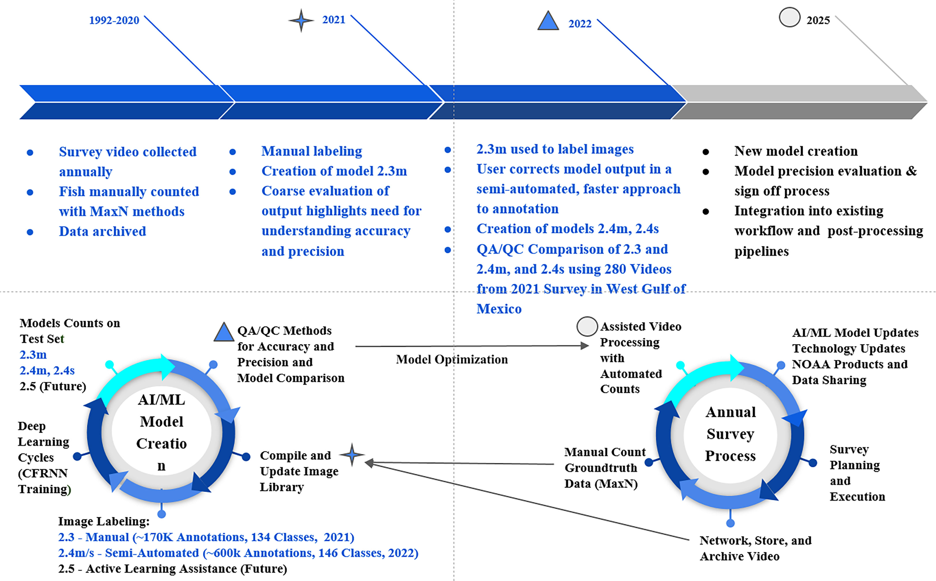
Figure 1 Combined workflow of model development and the annual survey process. MaxN manual counts are the maximum number of the same species, observed in the same frame, during a 25-minute station video. Model nomenclature “s” denotes single-frame fish tracking algorithms and “m” denotes motion-based tracking. Models 2.4s and 2.4m are available in a GitHub repository (https://github.com/VIAME/VIAME). These models are also available for public use as embedded pipelines on the VIAME web application.
For the fully manual training stage (hereafter ‘manual’) of the machine learning process, we compiled the initial image library with 61.5k frame extractions from 2018 and 2019 surveys with no discrimination towards species or video station locations. Frames were extracted from videos at variable rates from 1 to 10 fps. In March of 2021 software was updated to include interface options to annotate video in addition to single frame imagery - leading to a rapid increase in the amount of annotations compiled in the training set. All annotations included in the training library were produced on videos with frame rates of at least 5 fps. During May of 2021, model 2.3 was developed with a library of 170,000 annotations across 135 classification groups (Figure 1). The data in this model was mostly labeled at the species level, but some classifications are at genus or family levels if identification cannot be determined with greater resolution. Model version 2.3 was deemed capable enough to shift the annotation efforts from the manual process, to a semi-automated process. Following six months of performing corrections on model 2.3 annotations, the training library vastly expanded to its current size at 603,533 annotations across 146 classification groups in order to train model iteration 2.4 (Figure 1).
Each model package has a set of configurations and pipeline files available that can be modified to optimize performance. To facilitate reproduction of these methods, the following paragraphs describe the model nomenclature and text designations within the configuration files that can be selected or altered for different application purposes.
There are designations for the size of video fed into networks including 0.5x, 1.0x, 2.0x. The 0.5x size processes videos at 640x640 pixels, 1.0 at native input resolution, and 2.0x increases image resolution by a factor of 2 to 2.5. All results reviewed here were generated at the 1.0x scale configuration for all models. The fish tracking pipelines have been created with two different types of models: motion (m) and single-frame (s). The 2.4m (motion) model is an updated version of 2.3m but uses a larger annotation library. Model 2.3 runs a CFRNN across two motion channels and native intensity. Model 2.4s (single-frame) is a single-frame detector (CFRNN without motion training), built on the same library as 2.4m, but across one optical intensity input channel.
All pipelines run two classifier models by default - a ‘big’ and ‘small’ classifier, which target larger and smaller fish (measured via raw pixel area) for better performance at each, using the ‘resnet’ or ‘resnext’ 50 and 101 architectures (He et al., 2016; Xie et al., 2017). Only one classifier is applied for a size dependent detection state. The small fish classifier and big fish classifier are based on the size of annotation boxes with limits that can be adjusted a priori. For all three model iterations compared in this study, the area pivots of positive 7000 and negative 7000 were used as a threshold to discriminate between “large” and “small” fish. This means that, in the pipeline, only one model is applied for each detection state, greater or smaller than 7000 pixels. When the localization area (width multiplied by height) of the bounding box is greater than or equal to 7000 square pixels, the big classifier is used; conversely, when less than 7000 square pixels are used, the small classifier is employed. When under the lower bound of 1000, no classifier is applied and the detection is labeled as an UNKNOWNFISH. The bound of 1000 was also arbitrarily selected, although it should be noted that these detections carry little weight if they occurred on the same track as larger detections. These classifiers were trained on only small and big area input chips, respectively, for improved classification performance in each condition. Model 2.3 employed resnext architecture for both the large and small classifier, while both 2.4 models used resnext101 for the large classifier, but resnet50 for the small classifier.
Automated counts from 315, 25-minute, videos from the 2021 GFISHER combined survey were generated using models 2.3, 2.4m, and 2.4s. Videos were annotated at a rate of 5 fps, yielding 7500 frames per video. The 315 videos were selected from stations west of the Mississippi River Delta (-89.5 W). With each object classification, VIAME estimates and provides a confidence value. The confidence score is calculated in eq 1.0:
OR
Variables are given as c = the class ID; n = total number of unique localizations along the frames of each track; deti = detection value for a particular state in a track frame i; fish_conf(t) = fish detection value for a particular state in track time t; clsi(c) = classifier value for class c at the track frame i; class_conf(t,c) = classifier confidence value for class c at time t; b = posterior probability that a track is definitely a fish [default = 0.1]. Automated counts at the model confidence thresholds (CTs) of 0.1, 0.2, 0.3, 0.4, 0.5, 0.6, 0.7, 0.8, 0.9, and 0.95 were used to filter VIAME output and then subsequently compared to manually derived and reviewed data sets for 280 stations (hereafter validation set). It is assumed in this analysis that the manual post-processing and estimates of MaxN counts are accurate. However it is important to understand that these are uncalibrated values, and thus our definition of validation set is reliant on this assumption until a field calibration method is devised. We base our analysis, and proposed QA/QC method, from otolith aging models outlined in Campana (2001). Calculations were executed with the FSA Analysis R script developed by Derek Ogle of Northland College (Ogle, 2013). In these calculations our automated counts by multiple models are analogous to age estimations of otoliths generated from multiple reads against the validation set. We calculate the percent of videos with exact agreement, percent of videos within 1 and 2 counts, the ratios of false-positive and false-negative detections, and model coefficient of variation (CV, %). For each increase in CT the number of stations used for calculations is reduced number of stations with 0 automated detections increases. Stations with zero fish detected in automated processing were removed from the analysis so total percent agreement would not be inflated by agreement of zero, given that most species only appear in a fraction of the videos. Species and model specific estimates are calculated at each CT level, for all stations with positive observations of the selected species (i.e. verified by manual post-processing). CV was calculated as illustrated in Campana (2001) and eq. 2.0 below:
where Xij is the ith count of the jth number of fish, Xj is the mean count of the jth number of fish, and R is the number of times each fish is counted (in this case 2 – one manual, one automated).
Finally, the ratio of false-positives was determined by dividing the number of stations with automated detections when the species was not present in the ground truth, over the total number of stations where the species was not present as determined by the validation set (proportion of stations with false detections). False-negatives were also determined by dividing the number of stations without automated detections when the species was present in the ground truth, over the total number of stations where the species was present (proportion of stations with undetected species). Correlation (r2) and slope were also calculated from the linear regression of manual versus automated model run output. Slope was used to evaluate if the linear relationship between manual and automated counts deviated from 1 (i.e. a 1:1 relationship), while correlation was used to evaluate variability about that predicted relationship.
We used a combination of false-positive rate (proportion), percent of exact count agreement (%), percent of data within 1-2 counts (%), and model CV (%) to assess model quality per species and provide guidance on confidence filters to apply in post-processing automated output from VIAME when using the models discussed in this paper (Figures 2–5; Table 1). Evaluation of these variables is considered collectively with more weight placed on reducing false-positives, percent of data within 1-2 counts, and model CV. For example, model 2.4s achieved a slightly higher percent agreement than model 2.4m for Vermilion Snapper (Rhomboplites aurorubens) at a CT of 0.4, but had a higher rate of false-positives than the similarly performing model 2.4m at a CT of 0.6 – thus 2.4m @ 0.6 was chosen as the optimal model for this species (Figure 6). Given those criteria, we determined that model 2.4s was the optimal model for 13 of the 23 evaluated species (Table 1). For 8 species, model 2.4m was optimal. Model 2.3m, performed better for the remaining two species. In general, model performance was greatly improved from model iteration 2.3 to 2.4 with both fish tracking methods and across most species. In contrast, cryptic Lionfish (Pterois sp.), the 2.4 models greatly reduced the amount of high-confidence false-positive detections. As a pattern for most species, counts were overestimated at low CTs, maximum percent agreement was achieved for CTs between 0.3-0.7, and counts were underestimated at high CTs (0.8-0.95). At the CTs showing maximum percent agreement, most of the species were undercounted, suggesting that the models tend to make conservative estimates in comparison to the validation set as CTs become more restrictive. This outcome is heavily influenced by applying more restrictive filter criteria (increased CT) because the sample available to analyze the data is reduced by definition (i.e. high CTs reduce detections and thus sample sizes to conduct analyses).

Figure 2 Percent Agreement of automated counts with top performing model 2.4s to expert derived counts for twelve commercially and ecologically important species of reef fish commonly observed in the Gulf of Mexico. Lines are labeled with the initials of the species name in the legend. Species with high percent agreement coupled with low false-positives and CV’s can potentially filter data with higher confidence values, whereas models with worse performance would use a decreased confidence value to filter data.
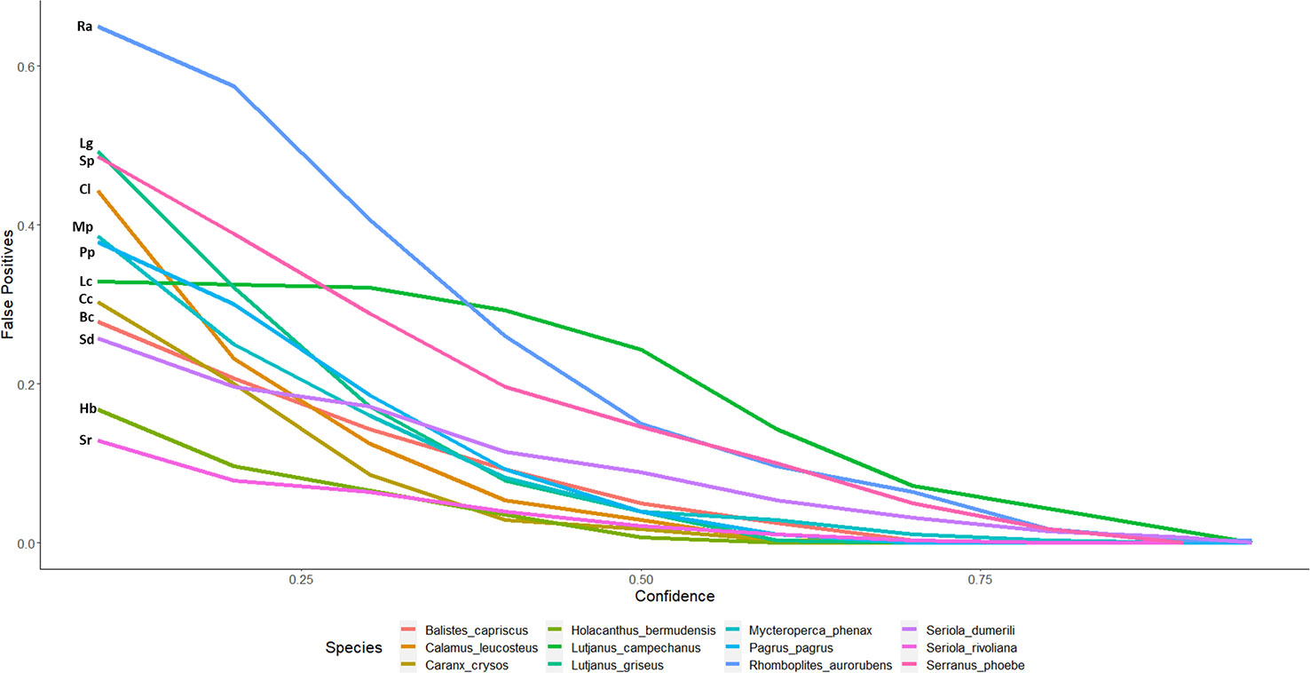
Figure 3 False-positive detections of automated counts with top performing model 2.4s to expert derived counts for twelve commercially and ecologically important species of reef fish commonly observed in the Gulf of Mexico. Lines are labeled with the initials of the species name in the legend. The false-positive ratio was determined by dividing the number of stations with automated detections when the species was not present in the ground truth, over the total number of stations where the species was not present as determined by the validation set.
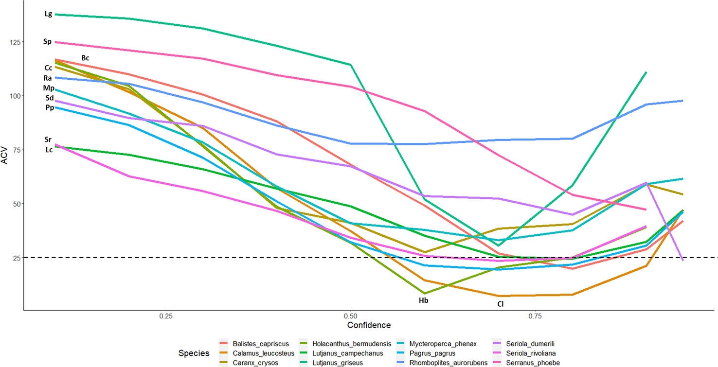
Figure 4 CV% for automated counts with top performing model 2.4s to expert derived counts for twelve commercially and ecologically important species of reef fish commonly observed in the Gulf of Mexico. Lines are labeled with the initials of the species name in the legend. Only 7 of 23 species make it below 25% threshold: B. capriscus, C. leucosteus, H. bermudensis, L. campechanus, P. Pagrus, S. dumerili, S. rivoliana.
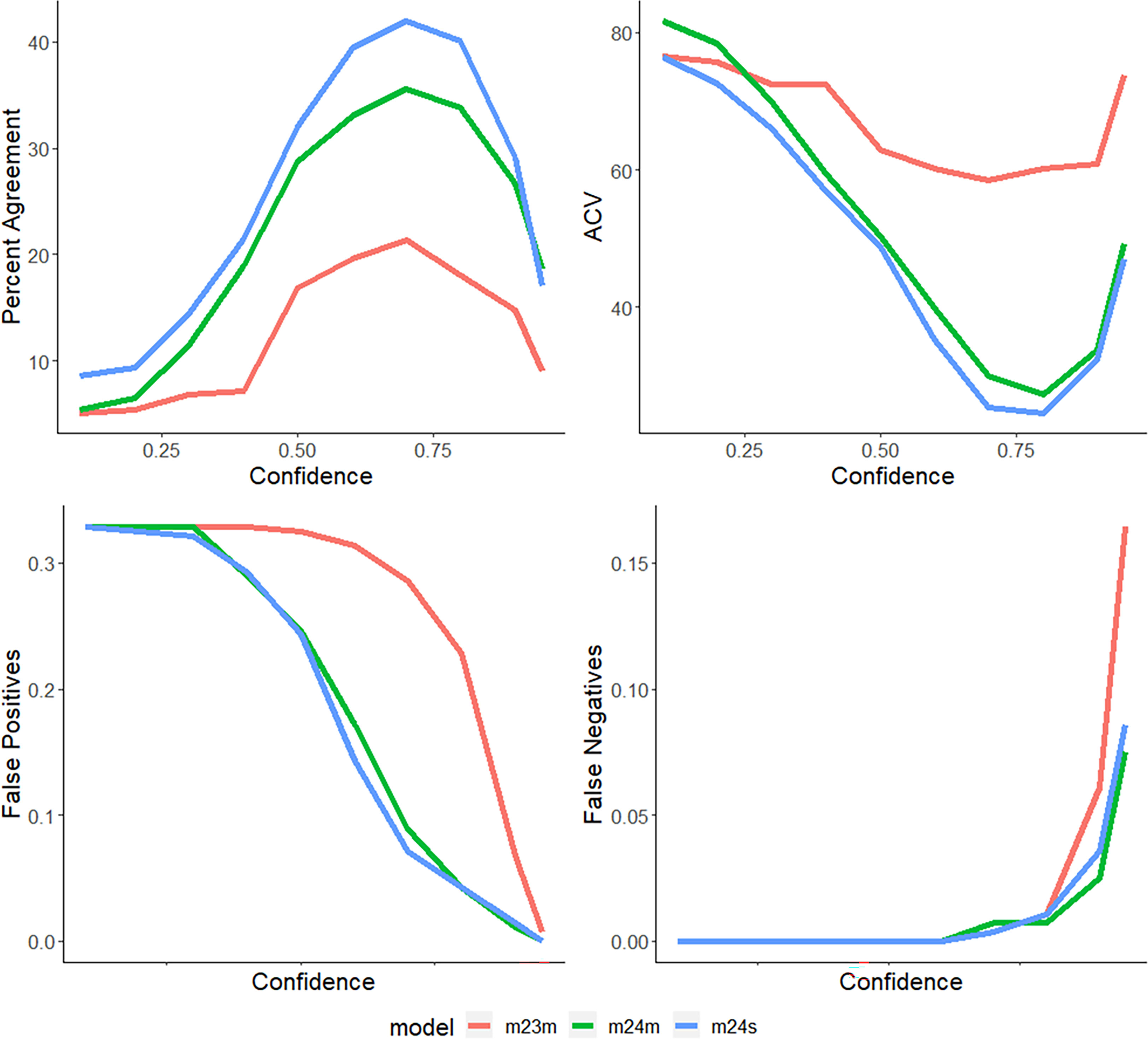
Figure 5 Percent agreement, ratio of false-positive detections, ratio of false-negative detections, and CV values across all confidences (0.1-0.95) for models 2.3, 2.4m, and 2.4s for (Lutjanus campechanus, the most observed species of the survey) with a maximum percent agreement of 42.03, and a minimum CV value of 24.5).
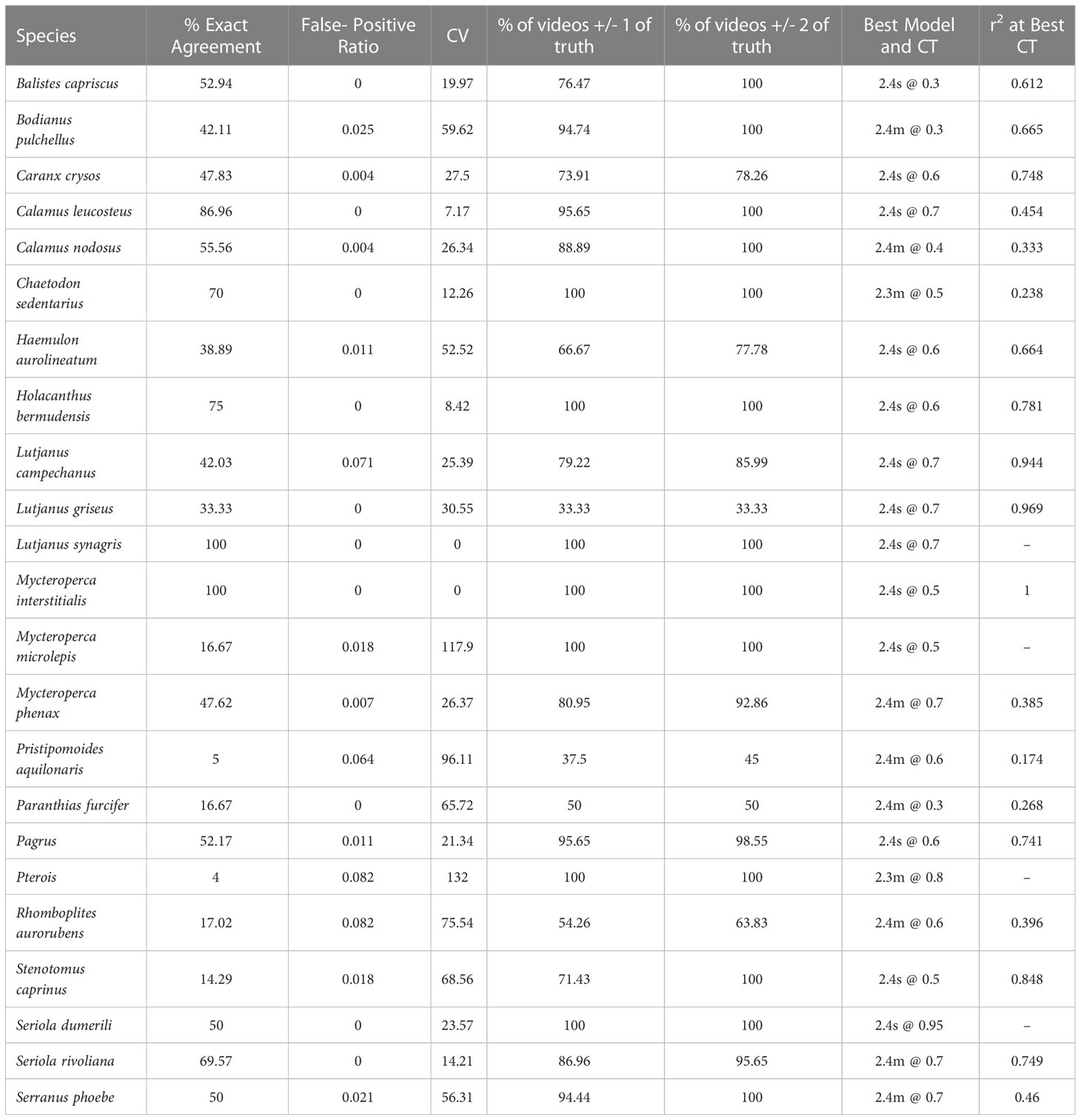
Table 1 Summary of model performance for 23 commercially and ecologically important species commonly observed in the 2021 SEAMAP Reef Fish Video Survey on reef structures along the shelf of the Gulf of Mexico West of the Mississippi River (< -89.5° W).
Figure 2 displays the percent agreement curves for model 2.4s counts across 12 of the most frequently observed species and are representative of diverse groups of fish. As most automated counts are initially overestimated, the ratio of false-positives is also greatest at low CTs and decreases with increasing thresholds and as low confidence identifications become filtered out (Figures 3, 5; Table 1). False-negatives were much less common than false-positives, but occur at a higher rate at high CTs. Whitebone Porgy (Calamus leucosteus) was the species that achieved the highest percent agreement (86.96) and lowest CV value (7.17), while reducing false-positives to zero. Some maximum percent agreements are reported as 100% (Table 1), however caution should be made in these interpretations as sample size is greatly reduced when using CT to filter out low confidence detections. While there is limited performance in percent exact agreement, automated counts for almost all species were within 1 of true counts for at least 50% of stations where the species was detected.
Strength of the linear relationship between automated and manual counts (r2) varied by species (0.2-0.9) and improved with increased observations in the data (Figures 6–8; Table 1). Correlation between automated and validation set counts was dependent upon the number of observations in the data set, site specific fish density, and life history patterns. For instance, Red Snapper showed high proportions of positive observations and yielded a strong enough correlation for symmetry tests to be conducted (Automated MaxN = Validation Set MaxN *(0.7) + 1, r2 = 0.9439). Results of that analysis indicate decreased reliability at sites with species specific counts >10. Thus model accuracy deteriorates with increasing site abundance, low count values were always more accurate, and most of the variability is contained to those high count values. For species with low counts, accuracy issues have less to do with site specific abundance and more to do with the training model itself. Scamp (Mycteroperca phenax), show weaker correlation than Red Snapper (Automated MaxN = Validation Set MaxN *(0.37) + 0.86, r2 = 0.3847), however have ~193k fewer annotations in the library (Figures 7, 8; Table 2). For all species, the slope of these best-confidence regression lines are less than one, which is an additional indication that the models conservatively undercount fish (a perfect model would have a slope = 1). Thus models would likely be less sensitive to increases in abundance depending on the frequency of high counts in the database.

Figure 6 Comparison of automated counts at the top performing model (2.4s) and confidence threshold (0.7) for Red Snapper, Lutjanus campechanus (the species with the most observations across all stations of the survey). Total agreement sample size (n) at confidence of 0.7 was 207. Residual standard error is 1.451 on 205 df. Linear regression is VIAME MaxN = Validation Set MaxN *(0.7) + 1 with r2 of 0.9439. F-statistic is 3450 on 1 and 205 df, p = 2.2e-16. 79.22% of counts within 1, and 85.99% were within 2 of validation set counts.
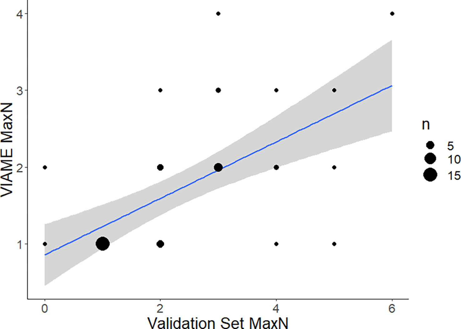
Figure 7 Comparison of automated counts at the top performing model (2.4m) and confidence threshold (0.7) for Scamp, Mycteroperca phenax (a commonly observed grouper species in the Gulf of Mexico). Total agreement n at confidence of 0.7 = 42. Residual standard error is 1.64 on 40 df. Linear regression is VIAME MaxN = Validation Set MaxN * (0.37) + 0.86 with R2 of 0.3847. F-statistic is 25.01 on 1 and 40 df, p-value is 1.81e-5. 80.95% of counts within 1 of ground truth, 92.86% within 2 of ground truth.
Figure 8 Comparison of automated counts at the top performing model (2.4m) and confidence threshold (0.6) for Vermilion Snapper, Rhomboplites aurorubens (a commonly observed snapper species in the Gulf of Mexico). Total agreement n at confidence of 0.6 = 94. Residual standard error is 16.8 on 92 df. Linear regression is VIAME MaxN = Manual MaxN (0.12) + 1.9 with R2 of 0.3963. F-statistic is 60.4 on 1 and 92 df, p-value is 1.073-11. 54.26% of counts within 1 of ground truth, 63.83% within 2 of ground truth.

Table 2 Count of annotations per species that contributed to the training library for each model and the difference in maximum percent agreement between iteration 2.3 and 2.4.
Increased annotations used to train models resulted in increased accuracy and precision in most cases; however there are species-specific complexities that confound results (Table 2). For example, while a 180% increase in annotations led to a strong increase in percent agreement and reduction in false-positives for C. leucosteus, model performance does not improve similarly in cryptic and schooling species. A 266% increase in annotations only resulted in a 1.76% improvement in maximum percent agreement for Lionfish. While model 2.4s could achieve 4.76% agreement for Pterois at a CT of 0.2, this was not selected as the best option, because low CT resulted in more false-positives than the best 2.3 model (which tracked 4% agreement at a confidence of 0.8). The smaller, fast-moving, and denser schooling species such as Wenchman (Prisitpomoides aquilonaris) and Vermilion Snapper (R. aurorubens) both had substantial increases in the number of annotations, but achieved less than 4% increases in percent agreement despite the massive increase in annotations used to train the models (Table 2). Model counts for Vermilion Snapper also produced poor linear regression fits (Automated MaxN = Manual MaxN *(0.12) + 1.9, r2 = 0.3963; Figure 6).
Our efforts to create automated, fish detection and classification algorithms, has highlighted the importance of understanding accuracy and precision using methods that analyze field-collected video against ground-truthed video collections as a complement to methods such as mAP that evaluate a subset of training data. Ideally this would be accomplished using a calibrated validation set but this level of understanding remains elusive at present. Estimation of accuracy and precision of AI/ML models is a crucial step towards their implementation and integration into existing post-processing frameworks because continuity of time series is critical for use in stock assessments. For instance, stock assessment models can now incorporate time varying catchability (Wilberg et al., 2009), and thus if a technology changes catchability (e.g. AI/ML catches things humans do not), abundance estimates have to be able to measure and compensate for that effect. Critically, current manual methods have been vetted via thorough review in assessment or publication outlets, and thus any automation of post-processing will have to be validated and precision metrics tracked through time, including estimates from historic video archives. Critically, this study assumes that human annotation produces accurate data, but the manual counts should not be treated as a calibrated set.
We demonstrate that model performance largely depended upon the number of classification specific annotations used in model training, fish density, and the incidence of various behaviors (e.g., schooling). Regardless of model iteration and application of a confidence filter on the data, model variability increased with increasing number of fish observed. This effect of decreasing precision with increased abundance is particularly pronounced for schooling or shoaling species of fish (e.g., Vermilion Snapper). Cryptic and small fish (e.g., Lionfish, Butterflyfish) were also problematic as they look very similar to the habitat and are often not detected, presumably because the algorithm believes them to be background (e.g., soft coral). Regardless of the underlying source of error, the method we propose here provides researchers with defined metrics to track model performance as a standard component of post-processing video data sets, will help external researchers evaluate model utility for other projects, and suggests species specific output filters for current SEFSC-VIAME models. We believe the current precision of our best model (2.4s) allows for implementation of a semi-automated approach to post-processing by pre-filtering low complexity videos (e.g., low abundance) for full automation and light QA/QC, versus those that will require more intensive manual processing. Thereby we can more efficiently direct manual annotation efforts, reduce time needed to generate usable data sets, and reduce potential effects of reader bias.
Mean Average Precision (mAP) is a standard metric for gauging model precision and is calculated by withholding a portion of the training set against which precision is estimated (Padilla et al., 2020). Efforts using a portion of the dataset (the library for iteration 2.2) reported a mAP50 value of ~70% for detection precision and achieved ~70% for top-class accuracy (Boulais et al., 2021). For model 2.4 detection precision was reported with a mAP50 of 79% for 2.4s, and 74% for 2.4m (supplementary 1). Our analysis clearly shows that additional metrics such as percent agreement, ratio of false-positive detections, and CVs, are necessary for understanding accuracy and precision of models run on naive videos as opposed to evaluation of a subset of training data. Further, these metrics are likely more valuable for implementation of automated methods for post-processing critical time-series survey data as they provide direct inference to performance against existing reads that can be thought of as validated annotations. This is especially true for generating count data for long term time-series containing long-length, high-resolution, and high frame-rate videos. We believe this because mAP scores are based on a selected level of intersection of union (IoU) between frames, and are therefore considered a measure of frame-based precision, rather than precision over the course of a video relative to counts (i.e. abundance). A high mAP, may not be indicative of a models capacity to produce accurate count estimates from novel unlabeled video sets (i.e., annual survey collection). Recent review of fish detection and monitoring methods (Barbedo, 2022) highlights the need for a standardized measurement of accuracy and precision between different models working in different applications, and especially the need for doing so with large sets of unlabeled data that represent natural conditions. This step towards standardization is ultimately necessary to build trustworthy models that can emulate humans in surveys and practical situations.
One of the more obvious results was that increases in training library size, and specifically to class specific annotations, resulted in improved model performance in general and within classes. Although sample size does generally increase model performance the resultant datasets can be imbalanced in the direction of ubiquitous species, an issue known as longtail distribution (Cai et al., 2021), and which is evident in the training library used in the set of projects dealing with this data set (Table 2, Boulais et al., 2021; Alaba et al., 2022). The longtail problem arises naturally from the imagery as ubiquitous species are frequently observed, and thus labeled, even from frames in which more rare species are being targeted. While the improvements to the models can be significant, those gains may not benefit all classes included in a model. In contrast, uniquely mottled and/or shaped taxa (e.g., Sheepshead – Archosargus probatocephalus) generally required fewer annotations to generate reasonable models than for species with conspecifics that share similar appearance (e.g., Scamp –Mycteroperca phenax and Yellowmouth Grouper – Mycteroperca interstitialis).
An approach to dealing with the longtail distribution problem is continued development and integration of active learning algorithms into the training process. Active learning algorithms include output that directs training towards the most important classes to add to the annotation library on which models are trained. Thus creating a focused training for species with fewer annotations and introducing better balance to the training set. Human supervision combined with active-learning algorithms can begin to produce true artificial intelligence systems that recognize what is not understood by the neural network and can autonomously generate new classes for the training library (Lv and Dong, 2022). Further discussion is required to determine whether there could be a longtail bias, based on this distribution of the annotation library, or if such bias should be integrated into model training since it is part of the natural system (Alaba et al., 2022). The fact that Red Snapper has the highest rate of false-positives of any species at the optimal CT (Table 1, Figure 3) may be evidence of longtail bias. Recent efforts (Dawkins et al., 2022) combined several large annotation datasets, including the annotation library used for iteration 2.4, to train an improved and versatile tracking model in VIAME. Following another round of library growth and training with these foci, model performance can again be compared to gauge improvements, along with any alternative architectures or competing model developments. For example, mathematical changes could be made to replace the fish detection output score, with a dedicated classifier which asks how well the fish is showing (i.e., a score given to each fish detection based on quality of the image in terms of the number of pixels and the fish orientation to the camera). The detector output is currently used as a surrogate because its score likely has some correlation with how well the fish is displayed, even though it wasn’t created explicitly for that purpose. Many other adjustments to parameters can be tested within the current model configurations due to the versatility of the VIAME software as a machine learning application. Capabilities currently exist to estimate lengths of fish and ongoing studies are using AI/ML for otolith age/length indices. Eventually combining these systems will lead to the future of AI/ML based governance in fisheries management. Given the increased performance of model 2.4s from 2.3, there should be a reduced cost in supervised correction effort, and therefore a more efficient path to a more proficient model 2.5 (Figure 1).
For some schooling and cryptic species, increasing the number of annotations in the training library was not entirely effective. For instance in the case of Vermilion Snapper the training library was increased 344% (Table 2), but model performance showed high variability, low percentage of exact counts, and high model CV (~75%, Table 1). Despite increased annotation, there was minimal improvement for Lionfish classification. We hesitate to speculate on the reasons for variable performance improvement with annotation increases, nor can we suggest methods to deal with this problematic bias, but challenges with high abundance obviously translates to issues for schooling species. The first suggestion is that knowing this bias, we can use this in a similar way to the VIAME generated CT data, to filter out videos for automation versus those that require more intensive supervision or a completely manual process. For instance if initial post-processing indicates a high number of tracks for Vermilion Snapper, we would pull that video for intensive QA/QC or fully manual processing. In all cases in which we see this kind of effect the frequency distribution of high-density sites indicates that these tend to be rare occurrences, and thus filtering in this fashion will result in decreased annotation time and effort. Recent efforts to mathematically deal with this issue were presented in Connolly et al. (2021). Another approach would be to train models to detect schools and create software functionality that would subset the portion of the image with the school to estimate a count (Li et al., 2022). Regardless of the approach taken there will be an obvious need to understand model performance especially at high abundance sites.
VIAME model output includes classification confidence information (i.e. CT) which can be used to filter model output and thereby optimize workflows by decreasing post-processing effort. The value of the CT itself is not used to determine model performance, but it may be important for gauging performance between models that will likely use increased training library sizes (2.3 vs 2.4), or with different training parameters (2.4m vs 2.4s). For instance, if the best confidence for a class is at 0.5 in model 2.3, but 0.7 in model 2.4, then that could be indicative of model improvement. Critically we observed that we can easily reduce false-positives by increasing confidence filters even in the worst performing models. These false-positives were common in model 2.3 and were often associated with clouds of turbidity (Figure 9), debris, parts of the camera array, and habitat structures. Whereas the incidences of false-positives were greatly reduced in model 2.4, likely as the result of improved training and better background identification. Thus, our method provides a general framework for fine-tuning VIAME output generated using the SEFSC models we presented in our analysis and that are hosted online (https://viame.kitware.com/#/root), as a tool to assist human readers in producing accurate counts and reduce post-processing effort (Table 1). Critically, the CT filter enables video annotators to focus on conditions and species that require more intensive review. For instance videos with few individuals and/or with high confidence species could be processed using automated methods and follow up quality control processing. Species with high percentages of automated counts within 1 of true counts will require minimal QA/QC compared to those with lower percentages. In contrast, models with high abundance and/or low confidence species would require a semi-automated approach with an intensive manual QA/QC process. Importantly for Red Snapper, the 2.4s model may reliably provide automated counts for stations in the West Gulf up to a MaxN of 10 fish. Of the 280 stations evaluated, 244 had counts <11 Red Snapper. Thus if a request were made for red snapper data we could reliably automate ~90% of the reads, leaving manual annotation to the remaining 10% plus a full QA/QC process to complete for all annotations. Further training and testing of larger sample sizes is required to establish reliability limits for other species. We anticipate as model performance improves through time, annotation speed will increase due to a reduction in effort during the quality control process.
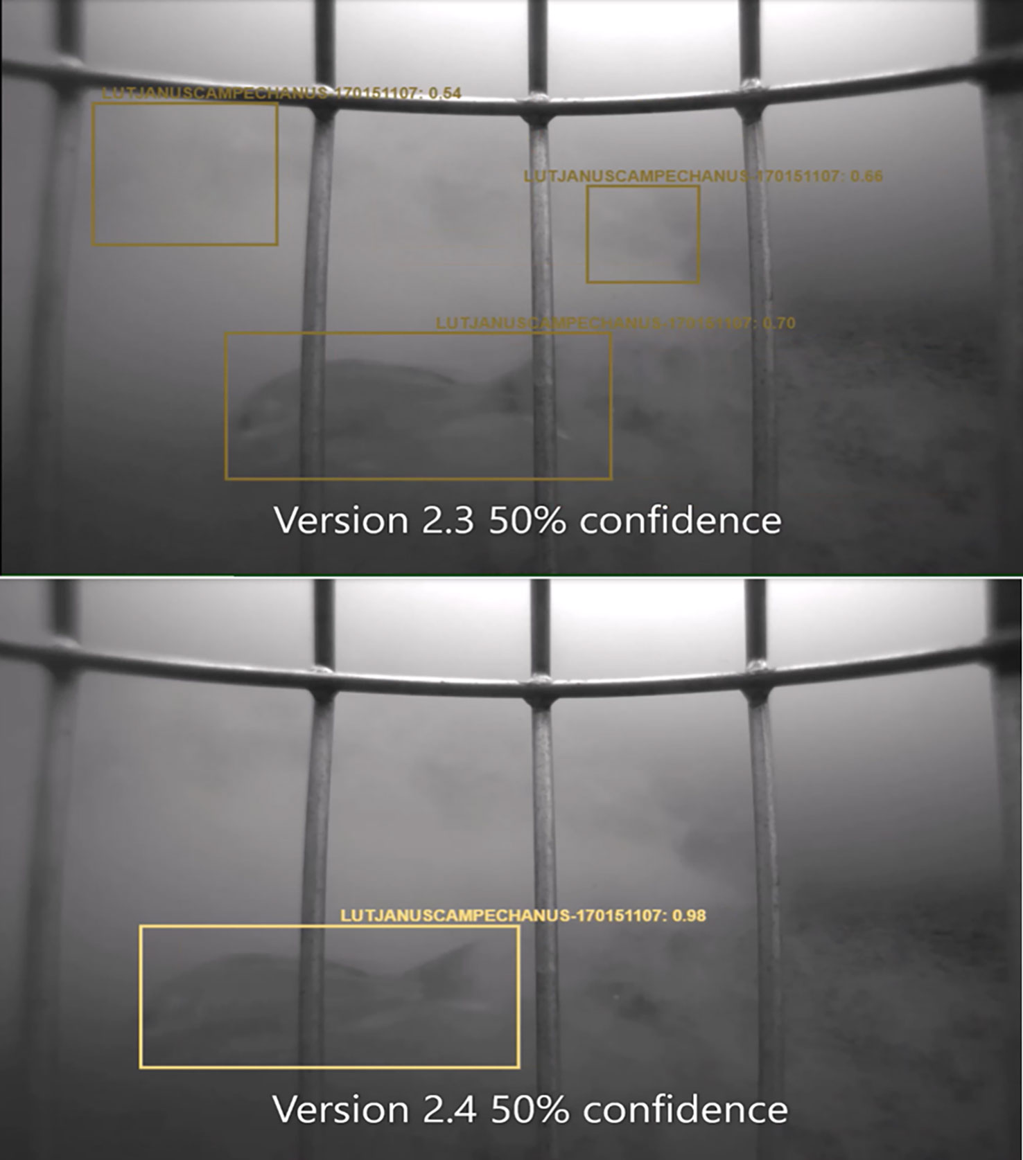
Figure 9 Example of reduction of false-positives and increase in confidence of detection and identification (Station 762101220 as turbidity plume clears the field of view). “50% confidence” in figure refers to the confidence threshold of the model.
There are also benefits for a reader viewing the low confidence VIAME detections, as sometimes the AI/ML algorithm is better at detecting minute differences, or was trained over a range of augmented orientations and shades simultaneously that enables classification on characters that a human may not have seen or be tuned to recognize. In cases where specific classification is not necessary VIAME has a general fish detector that can be helpful for generating counts and for visualizing individual fish. We believe methods outlined here will provide researchers a consistent and robust method by which model performance can be evaluated as technology, both on the camera and algorithm sides, continues to improve. Importantly, this approach provides a method by which future model performance can be gauged. In the case that ecosystem based management processes require improved assemblage data, the automated methods provided here would offer precision metrics that are invaluable in calibrating and tuning ecosystem models. Moreover, the proposed methods here for a QA/QC process could be adapted to any type of machine learning model development in the future, and could be beneficial both inside and outside of fisheries research to ensure globally cooperative systems of trustworthy AI.
Future efforts for model improvement must include increased annotation for species that demonstrated high levels of misclassification rates, decreased matching to exact counts, and increased CV values. Methods that bring balance into the training model are therefore needed such as the queried learning or longtail alleviation approaches mentioned earlier (Alaba et al., 2022). Conversely, effort should not be expended on increasing annotations for species with associated high precision models. Many observed species have low levels of percent agreement and high levels of false-positives, whereas many others have not yet been annotated in the training library. Thus a deliberate analysis that highlights those species is needed to help direct efforts to improve the image library itself. At times ‘handoffs’ occur when one or more fish cross paths and causes track identity to switch among individuals (i.e. more than one individual included in a single track). This can result in misclassification to the wrong species which we hope to address with the global tracking model. Dense schools have not been annotated and represent a gap in the annotation library. Schools of baitfish (e.g., Scad – Figure 10), even smaller than Vermilion Snapper, will likely require alternative annotation methods that allow for density estimation rather than individual tracking. Other issues such as gaps in tracks, double-boxing of single individuals, and single-boxes on multiple individuals can also occur but are mostly nuisances and should reduce as software and algorithms improve. Automated workflows show promise in these early phases of development, but for many of the reasons highlighted here it is our opinion they will always require some variety of human oversight, thus frameworks that include model metadata and performance against validation sets need to be developed in concert with the algorithms themselves.
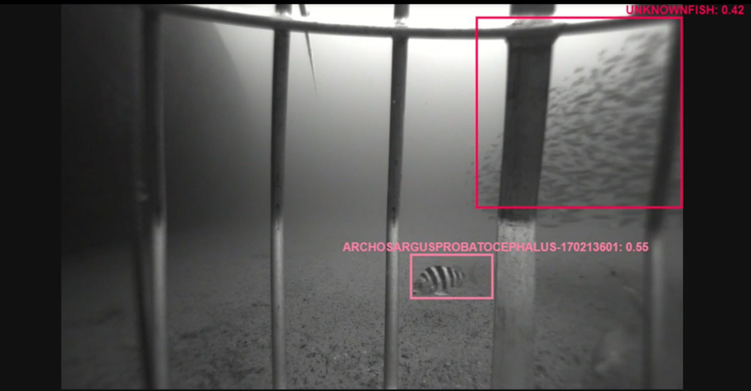
Figure 10 Example of a successful detection of a Sheepshead (Archosargus probatocephalus) with juxtaposition to the breakdown of performance with large schools of small, less distinguishable fish (Scad).
Accuracy and precision present significant hurdles for the implementation of automated processes, but nearly as important will be realizing the benefits of automation in reduced annotation time. The track-based annotation and modeling can provide more accurate identifications because they are derived from multiple frames strung together to create a majority-vote classification over many frames. A single correction of a track, corrects all annotations associated with the track in a single pass and the end result is decreased post-processing time. Using this method increases the number of images, fish angles, and light conditions used to classify fish, and therefore is theoretically increasing classification agreement. It is also beneficial from a memory-cost standpoint. One 25-minute video, which is 7500 frames at 5 fps, is compressed to 1.17 GB (camera specifications from this survey) but when extracted as 7500 individual PNG files, it amounts to 9.84 GB. This reduction in memory is due to the ability to exploit correlation between frames in storing video. (Jain, 1989). Critically, because VIAME produces frame level counts and identifications, any current metric in the literature can likely be produced (e.g., MaxN, MeanCount, Time-At-First-Arrival, etc). This will have the additional benefit of facilitating analysis on the use of the various derived metrics and perhaps others not yet conceived.
Our translation of the otolith aging methodology for use in estimating the accuracy and precision of automated image analysis models shows promise as a means to ensure data quality for time-series creation and for both existing and anticipated data analysis needs. Model precision and agreement varied by species, number of annotations used in the training set, and only slightly by choice in tracking model (motion or single frame). CV comparisons have historically been acceptable up to around 10% in the otolith aging literature (Campana, 2001). Few of the CV values of the presented species with acceptable sample sizes fall in to this acceptable range in this analysis – only 7 of 23 species have CVs less than 25%, and only 2 are less than 10% (Figure 4). However, for this new application of these quality control methods, it must be decided if those are applicable in this example or determine what level is acceptable. There is a significant amount of investigation still needed on this topic, but we believe the framework presented here is a good first step towards establishment of best practices for integration of automated image post-processing into existing standard-operating-procedures.
Advanced technology, in particular miniaturization of computing and sensors, is providing researchers with data and insights into marine systems that were previously inaccessible. These technological advancements are both a boon, in that enormous amounts of data can be collected, but simultaneously present significant bottlenecks often due to being limited to manual post-processing methods (i.e. most data is in storage). Therefore, it is clear that AI/ML will be a significant component of marine laboratory toolkits to help facilitate post-processing necessary for further analysis and optimal use of datasets. This is particularly important in situations for which data timeliness is an important consideration for management decision making processes. Our experience over the course this investigation is that AI/ML has shown significant progress in utility, enough that we believe their integration into post-processing pipelines is a logical next step in the near future (e.g. 5-10 years). Our advice for researchers interested in deployment of AI/ML in optical post-processing is to develop accuracy and precision metrics in concert with the models themselves. This step is critical as many iterations of models can be simultaneously developed, but for their proper deployment their effectiveness has to be measured objectively. Our method presented here offers a way to judge model performance by evaluating model accuracy and precision against ground-truthed video sets. The method assumes a linear relationship between ground-truthed and automated counts and thus we have a simple model by which we can evaluate bias and drift as annual collections are analyzed and new versions of AI/ML models are developed. While the future is bright there remains significant hurdles associated with cryptic, schooling species, and with those having similar looking conspecifics. Some problems are likely going to be resolved by increasing the number of class specific annotations for rare species (e.g. gag) and bringing balance to training libraries, whereas solutions for schooling species are not as obvious and are potentially a limit of the technology. In addition to implementing model QA/QC protocols, programs that are looking to integrate automation into post-processing pipelines should also look to build equivalent manual data sets over an overlapping period of time to evaluate conservation of important time-series data.
MD does not imply a NOAA endorsement of Kitware or products and services related to the VIAME software.
The datasets presented in this study can be found in online repositories. The names of the repository/repositories and accession number(s) can be found below: https://github.com/VIAME/VIAME - The Git Hub page for VIAME software. Reference: SEFSC 100-200 Class Fish Models, All OS. Full video datasets and count data are available upon request.
JP, MC, and MD contributed to conception and design of the study. JP, MC, and JS organized the database. JP, JS, AF, and KR performed expert video annotation and ground truth reviews. JP and MC performed the statistical analysis. JP wrote the first draft of the manuscript. JP and MC wrote sections of the manuscript. All authors contributed to the article and approved the submitted version.
Funding was provided through Federal Marine Fisheries Initiative (MARFIN) Grant 20MFIH002 through NOAA’s National Marine Fisheries Service and the associated award NA21OAR4320190 to the Northern Gulf Institute from NOAA’s Office of Oceanic and Atmospheric Research, U.S. Department of Commerce. At sea data collections were funded by Southeast Fisheries Science Center base funds, and the RESTORE act funded Gulf Fishery Independent Survey of Habitat and Ecosystem Resources (GFISHER) grant number NA19NOS4510192.
The first author would like to acknowledge the efforts of all other authors in guidance to this point. The data could not be analyzed without having first been collected by NOAA research vessels Southern Journey and Pisces, and all those who contributed to the at-sea surveys. In addition, this study would not be possible without the continued technical support from VIAME software developers.
Author MD was employed by Kitware, Inc. Author JS was employed by Technical and Engineering Support Alliance (TESA) ProTechContract Company (JV).
The remaining authors declare that the research was conducted in the absence of any commercial or financial relationships that could be construed as a potential conflict of interest.
All claims expressed in this article are solely those of the authors and do not necessarily represent those of their affiliated organizations, or those of the publisher, the editors and the reviewers. Any product that may be evaluated in this article, or claim that may be made by its manufacturer, is not guaranteed or endorsed by the publisher.
The Supplementary Material for this article can be found online at: https://www.frontiersin.org/articles/10.3389/fmars.2023.1150651/full#supplementary-material
Alaba S. Y., Nabi M. M., Shah C., Prior J., Campbell M. D., Wallace F., et al. (2022). Class-aware fish species recognition using deep learning for an imbalanced dataset. Sensors 22 (21), 8268. doi: 10.3390/s22218268
Allken V., Rosen S., Handegard N. O., Malde K. (2021). A real-world dataset and data simulation algorithm for automated fish species identification. Geosci. Data J. 8 (2), 199–209. doi: 10.1002/gdj3.114
Bacheler N. M., Shertzer K. W. (2015). Estimating relative abundance and species richness from video surveys of reef fishes. Fish. Bull. 113, 15–26. doi: 10.7755/FB.113.1.2
Barbedo J. C. A. (2022). A review of the use of computer vision and artificial intelligence for fish recognition, monitoring, and management. Fishes 7, 335. doi: 10.3390/fishes7060335
Boulais O., Alaba S., Yu J., Iftekhar A., Zheng A., Prior J., et al. (2021). “SEAMAPD21: a large-scale reef fish dataset for fine-grained categorization,” in The Eighth Workshop on Fine-Grained Visual Categorization – CVPR21.
Cai Z., Vasconcelos N. (2018). “Cascade r-CNN: Delving into high quality object detection,” in 2018 IEEE/CVF Conference on Computer Vision and Pattern Recognition, Salt Lake City, UT, USA. 6154–6162. doi: 10.1109/CVPR.2018.00644
Cai J., Wang Y., Hwang J.-N. (2021). “ACE: Ally complementary experts for solving long-tailed recognition in one-shot,” in 2021 IEEE/CVF International Conference on Computer Vision (ICCV). 1–10.
Campana S. E. (2001). Accuracy, precision and quality control in age determination, including a review of the use and abuse of age validation methods. J. Fish Biol. 59, 197–242. doi: 10.1111/j.1095-8649.2001.tb00127.x
Campbell M. D., Pollack A. G., Gledhill C. T., Switzer T. S., DeVries D. A. (2015). Comparison of relative abundance indices calculated from two methods of generating video count data. Fish. Res. 170, 125–133. doi: 10.1016/j.fishres.2015.05.011
Cappo M., Harvey E., Shortis M. (2007). Counting and measuring fish with baited video techniques – an overview. Aust. Soc. Fish Biol. 2006 Workshop Proc. 1, 101–114.
Chuang M., Hwang J., Williams K., Towler R. (2014). Tracking live fish from low-contrast and low-frame-rate stereo videos. IEEE Trans. Circuits Syst. Video Technol. 25 (1), 167–179. doi: 10.1109/TCSVT.2014.2357093
Connolly R., Fairclough D., Jinks E., Ditria E., Jackson G., Lopez-Marcano S., et al. (2021). Improved accuracy for automated counting of a fish in baited underwater videos for stock assessment. Front. Mar. Sci. 8. doi: 10.3389/fmars.2021.658135
Cui S., Zhou Y., Wang Y., Zhai L. (2020). Fish detection using deep learning. Appl. Comput. Intell. Soft Computing 2020, 1–13. doi: 10.1155/2020/3738108
Dawkins M., Campbell M. D., Prior J., Faillettaz R., Simon J., Lucero M., et al. (2022). FishTrack22: An ensemble dataset for multi-object tracking evaluation. Second Workshop Comput. Vision Anim.
Ding J., Li X., Gudivada V. N. (2017). Augmentation and evaluation of training data for deep learning. IEEE Int. Conf. Big Data (Big Data), 2017, 2603–2611. doi: 10.1109/BigData.2017.8258220
Ditria E. M., Lopez-Marcano S., Sievers M., Jinks E. L., Brown C. J., Connolly R. M. (2020). Automating the analysis of fish abundance using object detection: Optimizing animal ecology with deep learning. Front. Mar. Sci. 7, 429. doi: 10.3389/fmars.2020.00429
Ellis D. M., DeMartini E. E. (1995). Evaluation of a video camera technique for indexing abundances of juvenile pink snapper, Pristipomoides filamentosus, and other Hawaiian insular shelf fishes. Fish. Bull. 93 (1), 67–77.
Garcia R., Prados R., Quintana J., Tempelaar A., Gracias N., Rosen S., et al. (2020). Automatic segmentation of fish using deep learning with application to fish size measurement. ICES J. Mar. Sci. 77 (4), 1354–1366. doi: 10.1093/icesjms/fsz186
He K., Zhang X., Ren S., Sun J. (2016). “Deep residual learning for image recognition,” in 2016 IEEE Conference on Computer Vision and Pattern Recognition (CVPR). 770–778. doi: 10.1109/CVPR.2016.90
Hsiao Y., Chen C., Lin S., Lin F. (2014). Real-world underwater fish recognition and identification using sparse representation. Ecol. Inf. 23, 14–21. doi: 10.1016/j.ecoinf.2013.10.002
Jennings S., Kaiser M. J. (1998). The effects of fishing on marine ecosystems. Adv. Mar. Biol. 34, 201–352. doi: 10.1016/S0065-2881(08)60212-6
Li J., Liu C., Lu X., Wu B. (2022). CME-YOLOv5: An efficient object detection network for densely spaced fish and small targets. Water 14 (15), 2412. doi: 10.3390/w14152412
Lopez-Marcano S., Turschwell M. P., Brown C. J., Links E. L., Wang D., Connolly R. M. (2022). Computer vision reveals fish behaviour through structural equation modelling of movement patterns. Res. Square Prelim. Rep., 1–24. doi: 10.21203/rs.3.rs-1371027/v1
Lopez-Vasquez V., Lopez-Guede J., Marini S., Fanelli E., Johnsen E., Aguzzi J. (2020). Video image enhancement and machine learning pipeline for underwater animal detection and classification at cabled observatories. Sensors 20, 726. doi: 10.3390/s20030726
Lv Q., Dong M. (2022). Active learning of three-way decision based on neighborhood entropy. Int. J. Innovative Computing Inf. Control 18 (2), 37–393. doi: 10.1016/j.ins.2022.07.133
Marini S., Fanelli E., Sbragaglia V., Azzurro E., Rio Fernandez J., Aguzzi J. (2018). Tracking fish abundance by underwater image recognition. Nat. Sci. Rep. 8, 13748. doi: 10.1038/s41598-018-32089-8
Marrable D., Barker K., Tippaya S., Wyatt M., Bainbridge S., Stowar M., et al. (2022). Accelerating species recognition and labelling of fish from underwater video with machine-assisted deep learning. Front. Mar. Sci. 9. doi: 10.3389/fmars.2022.944582
Ogle D. (2013). fishR vignette – precision and accuracy in ages (Ashland, Wisconsin, United States: Northland College).
Padilla R., Netto S. L., da Silva E. A. B. (2020). “A survey on performance metrics for object-detection algorithms,” in IEEE International Conference on Systems, Signals, and Processing (IWSSIP), Vol. 2020. 237–242. doi: 10.1109/IWSSIP48289.2020.9145130
Priede I. G., Bagley P. M., Smith A., Creasey S., Merrett N. R. (1994). Scavenging deep demersal fishes of the porcupine seabight, north-east Atlantic: observations by baited camera, trap and trawl. J. Mar. Biol. Assoc. United Kingdom 74 (3), 481–498. doi: 10.1017/S0025315400047615
Salman A., Siddiqui S., Shafait F., Mian A., Shortis M., Khurshid K., et al. (2020). Automatic fish detection in underwater videos by a deep neural network-based hybrid motion learning system. ICES J. Mar. Sci. 77 (4), 1295–1307. doi: 10.1093/icesjms/fsz025
Shafait F., Mian A., Shortis M., Ghanem B., Culverhouse P., Edgington D., et al. (2016). Fish identification from videos captured in uncontrolled underwater environments. ICES J. Mar. Sci. 73 (10), 2737–2746. doi: 10.1093/icesjms/fsw106
Tabak M., Norouzzadeh M., Wolfson D., Newton E., Boughton R., Ivan J., et al. (2020). Improving the accessibility and transferability of machine learning algorithms for identification of animals in camera trap images: MLWIC2. Ecol. Evol. 10, 10374–10383. doi: 10.1002/ece3.6692
Thompson K. A., Switzer T. S., Chirstman M. C., Keenan S. F., Gardner C. L., Overly K. E., et al. (2022). A novel habitat-based approach for combining indices of abundance from multiple fishery-independent video surveys. Fish. Res. 247, 106178. doi: 10.1016/j.fishres.2021.106178
van Helmond A. T. M., Mortensen L. O., Plet-Hansen K. S., Ulrich C., Needle C. L., Oesterwind D. (2020). Electronic monitoring in fisheries: lessons from global experiences and future opportunities. Fish 21, 162–189. doi: 10.1111/faf.12425
Villon S., Chaumont M., Subsol G., Villéger S., Claverie T., Mouillot D. (2016). “Coral reef fish detection and recognition in underwater videos by supervised machine learning: comparison between deep learning and HOG+SVM methods,” in International Conference on Advanced Concepts for Intelligent Vision Systems, Vol. 2016. 160–171.
Wilberg M. J., Thorson J. T., Linton B. C., Berkson J. (2009). Incorporating time-varying catchability into population dynamic stock assessment models. Rev. Fish. Sci. 18 (1), 7–24. doi: 10.1080/10641260903294647
Xie S., Girshick R., Dollár P., Tu Z., He K. (2017). “Aggregated residual transformations for deep neural networks,” in 2017 IEEE Conference on Computer Vision and Pattern Recognition (CVPR). 5987–5995. doi: 10.1109/CVPR.2017.634
Keywords: fisheries, machine learning, BRUVS, Maxn, Gulf of Mexico, automation
Citation: Prior JH, Campbell MD, Dawkins M, Mickle PF, Moorhead RJ, Alaba SY, Shah C, Salisbury JR, Rademacher KR, Felts AP and Wallace F (2023) Estimating precision and accuracy of automated video post-processing: A step towards implementation of AI/ML for optics-based fish sampling. Front. Mar. Sci. 10:1150651. doi: 10.3389/fmars.2023.1150651
Received: 24 January 2023; Accepted: 20 March 2023;
Published: 04 April 2023.
Edited by:
Hongsheng Bi, University of Maryland, United StatesReviewed by:
Abdelouahid Bentamou, Ecole Des Mines De Saint-Etienne, FranceCopyright © 2023 Prior, Campbell, Dawkins, Mickle, Moorhead, Alaba, Shah, Salisbury, Rademacher, Felts and Wallace. This is an open-access article distributed under the terms of the Creative Commons Attribution License (CC BY). The use, distribution or reproduction in other forums is permitted, provided the original author(s) and the copyright owner(s) are credited and that the original publication in this journal is cited, in accordance with accepted academic practice. No use, distribution or reproduction is permitted which does not comply with these terms.
*Correspondence: Jack H. Prior, amFjay5wcmlvckBub2FhLmdvdg==; amhwMjc3QG1zc3RhdGUubmdpLmVkdQ==
Disclaimer: All claims expressed in this article are solely those of the authors and do not necessarily represent those of their affiliated organizations, or those of the publisher, the editors and the reviewers. Any product that may be evaluated in this article or claim that may be made by its manufacturer is not guaranteed or endorsed by the publisher.
Research integrity at Frontiers
Learn more about the work of our research integrity team to safeguard the quality of each article we publish.