An automatic identification algorithm of internal solitary wave for mooring data based on geometric characteristics of the flow field

Internal solitary wave (ISW) is one of the most important sub-mesoscale phenomenas in the ocean, and detection of which is of utmost significance for marine exploitation, ecological environment protection and military affairs. Therefore, in this study, an automatic algorithm for the identification of ISWs was proposed based on the geometric characteristics of the flow field. The algorithm was applied to calculate the characteristic parameters of the ISWs and its reliability was further verified, indicating that the algorithm can effectively detect the ISWs and provide a reference for preventing and avoiding ISWs in ocean engineering.

1 Introduction

Internal waves are sub-mesoscale waves caused by seawater disturbances with stable density stratification, thereby leading to changes in the total water depth (Xu, 1999). The near-inertial internal waves, internal tidal waves, and internal solitary waves are different kinds of internal waves. As one of the most common internal waves, the internal solitary wave (ISW) is characterized by large amplitude, nonlinearity, and approximating constant wave propagation. In the past few decades, a large number of the ISWs have been observed in the South China Sea (SCS), especially in northeastern SCS (Liu and Hsu, 2004; Zhao, 2004), making SCS a hot spot for studying ISWs. The propagation and breaking of ISWs can lead to strong ocean mixing and promote the transport of nutrients and chlorophyll, thereby impacting the marine ecological environment (Wang et al., 2007; Cai, 2015; Dong et al., 2015). On the one hand, the resuspension and transport of seafloor sediment induced by the shoaling ISWs can change the seafloor topography (McPhee-Shaw, 2006; Masunaga et al., 2016; Tian et al., 2021a). On the other hand, the strong shearing stress of the shoaling ISWs can lead to sand wave and even seabed failure (Ma et al., 2016; Rivera-Rosario et al., 2017; Tian et al., 2021b; Tian et al., 2022). Moreover, the propagation of the ISWs can lead to strong convergence and divergence of the sea surface or sudden strong currents in local seawater. In turn, these currents can lead to large fluctuations in the isopycnal surface (Wu et al., 2022), thereby posing a great threat to the safety of sonar systems, submarines, offshore oil boring platforms, and other facilities (Osborne et al., 1978; Ebbesmeyer et al., 1991; Bole et al., 1994; Cai et al., 2003; Chiu et al., 2004; Duda et al., 2004; Yuan et al., 2013). Therefore, the early warning and prediction of the ISWs are of utmost necessity for marine resource exploitation, ecological environment protection, engineering, and military affairs.

The identification and detection of the ISWs is the primary objective of the early warning system. At present, the methods of the ISW detection mainly include spaceborne Synthetic Aperture Radar (SAR) and shipborne nautical X-band radar. The advantages of SAR are that it is capable of all-weather detection throughout the day with high resolution. The ISWs show different characteristics under different frequency ranges and polarization, which is conducive to the identification of the ISWs (Guo, 2020). According to the modulation characteristics of sea-surface waves due to the ISWs, large-scale remote sensing imaging can be carried out using an electromagnetic wave imaging mechanism for obtaining the spatial location, wavelength, direction, and other horizontal parameters of the ISWs (Alpers, 1985; Yang et al., 2000; Hong et al., 2015). However, due to the limitations of the satellite revisit period and the influence of harsh sea conditions, the ISW signals obtained by the satellite are usually accidental. Shipborne nautical X-band radar is an active microwave imaging radar with the advantages of high resolution and real-time monitoring. The X-band radar can effectively detect weak sea-surface wave signals, and then reflect the propagation speed and direction of the ISWs based on Radon transform techniques (Murphy, 1986). However, in practical applications, radar images are generally corrupted by noises such as clouds and sea waves. Therefore, noise suppression in radar images has become utmost necessary.

On the one hand, the early warning of the ISWs must ensure timeliness and real-time data. On the other hand, the near-surface current velocity is a major factor affecting the force loads on offshore structures (Li et al., 2016). However, the above two methods are not capable of velocity quantification, and cannot provide good services for engineering applications. Therefore, mooring observation is still the most direct and effective method of the ISW detection. The underwater fine structure and evolution characteristics of the ISWs can be directly analyzed from mooring observations. In terms of the prediction of the ISWs, Tian et al. (2023) proposed a method for predicting the shear stress induced by shoaling ISWs base on machine learning, and provide reference for reducing damage to the seabed caused by the ISWs. In terms of the real-time warning of the ISWs, only a few research studies (Yuan et al., 2013; Li et al., 2016) on the operational forecast of the ISWs in the SCS were conducted. By providing the mooring with the satellite instant communication system, the mooring data and the parameters of the ISWs can be obtained in real-time. However, as the initial and key work of the ISW prediction, the identification of the ISWs is mostly based on subjective judgment with experience and the auto-monitoring system has not been established so far. Therefore, in this study, an automatic identification algorithm of the ISWs was proposed based on mooring observation for the real-time automatic monitoring of the ISWs in the SCS. The application of the algorithm to observational data was evaluated systematically. The results indicated that the algorithm is reliable and can be applied to the precise prediction of the ISWs. The remainder of this study is structured as follows. The datasets and methods used in this study are highlighted in Section 2. The applications of the algorithm and the results of the analysis are discussed in Section 3. Finally, the summary and discussion of the study are presented in Section 4.

2 Data and methods

2.1 Data

The submersible mooring system was deployed on the continental slope lying west of the Dongsha Islands in the northern SCS. The mooring systems consisted of five major instruments, namely, SeaBird SBE-56 Temperature logger (T), SeaBird SBE-37SM MicroCAT Conductivity-Temperature-Depth (CTD) recorder, AANDERAA SeaGuard RCM recording current meter (AANDERAA), Upward-looking Teledyne RD Instruments (TRDI) Workhorse Long Ranger 75 kHz Acoustic Doppler Current Profiler (ADCP), and downward-looking TRDI Workhorse Sentinel 300 kHz ADCP. The sample interval of both CTDs and Ts were 30 s, and those of AANDERAAs was 2 min. Both 75 kHz and 300 kHz ADCPs sampled every 3 min with a bin of 8 m. The temperature accuracy of CTDs and Ts are °C. The velocity accuracy of ADCPs and AANDERAA are $\pm 1.0\%$ of measured velocity $\pm 0.5$ cm/s and 0.15 cm/s, respectively. The detailed settings of each mooring are shown in Figure 1 and Table 1.

FIGURE 1

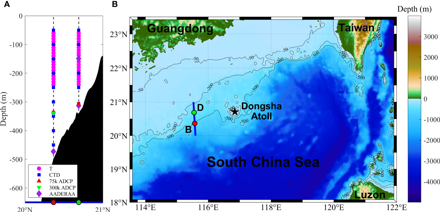
Figure 1 (A) Cross-section of the moorings B, D on the continental slope [blue line in (B)] and instruments deployed on each mooring and (B) topography of the northern SCS. The locations of the two moorings are indicated by red and green dots. The depths of T (magenta circle), CTD (blue square), upward looking 75kHz ADCP (red triangle), downward-looking 300kHz ADCP (green triangle), and AANDERAA (purple diamond) are also depicted.

TABLE 1

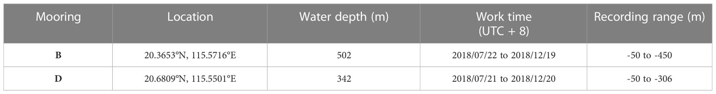
Table 1 Detailed settings of each mooring.

It should be noted that the environmental parameters such as temperature and salinity were not measured near the sea surface at the mooring station. Therefore, the monthly data from World Ocean Atlas 2018 (WOA18) was used as a supplement in the next section.

2.2 Theoretical models of the ISW

At present, Kortweg-de Vries (KdV) equation (Korteweg and De Vries, 1895) is the most commonly used nonlinear equation to describe the ISWs, which can be explained by the balance between weak nonlinearity and weak dispersion. The KdV equation for arbitrary vertical stratification of ocean density and background shear flow is expressed by the following equation (Holloway et al., 1997; Pelinovsky et al., 2007):

$\begin{array}{ll}\frac{\partial \eta }{\partial t}+(c_0+\alpha \eta )\frac{\partial \eta }{\partial x}+\beta \frac{{\partial }^3\eta }{\partial x^3}=0& (1)\end{array}$

where $\eta (x, t)$ represents the displacement of the pycnocline, $c_0$ is the linear phase speed, $\alpha$ is the nonlinear coefficient, and $\beta$ is the dispersion coefficient. $\alpha$ and $\beta$ are determined by the background density and horizontal velocity profiles, which are given by Equations 2 and 3, respectively.

$\begin{array}{ll}\alpha =\frac{3{\int }_{-H}^0{(c_0-U)}^2{(d\varphi /dz)}^{3}dz}{2{\int }_{-H}^0(c_0-U){(d\varphi /dz)}^{2}dz}& (2)\end{array}$

$\begin{array}{ll}\beta =\frac{{\int }_{-H}^0{(c_0-U)}^2{\varphi }^{2}dz}{2{\int }_{-H}^0(c_0-U){(d\varphi /dz)}^{2}dz}& (3)\end{array}$

where $H$ is the depth of local seawater, $U(z)$ represents the background shear flow in the wave direction, and $\varphi (z)$ represents the modal function of vertical displacement. In this case, $\varphi (z)$ is normalized, and its maximum is given by ${\varphi }_{max}=1$. As shown in Equation 4, $c_0$ and $\varphi (z)$ can be derived from the Taylor-Goldstein (T-G) equation (Apel et al., 1995; Grimshaw et al., 2010):

$\begin{array}{ll}\frac{d}{dz}\left[{(c_0-U)}^2\frac{d\varphi }{dz}\right]+N^2\varphi =0& (4)\end{array}$

$\begin{array}{ll}\varphi (-H)=\varphi (0)=0& (5)\end{array}$

where $N(z)$ represents Brunt-Väisälä frequency, and $z$ is the vertical coordinate, and is positive upward.

The stationary solution of the KdV equation is given by the following equation ($x$ -axis is positive eastward):

$\begin{array}{ll}\eta (x,t)={\eta }_{0}sec{h}^2\left(\frac{x+ct}{L}\right)& (6)\end{array}$

where ${\eta }_0$ is the maximum amplitude of ISW (${\eta }_0<0$ indicates the concave type of ISW and ${\eta }_0>0$ indicates the convex type of ISW), $c=c_0+\alpha {\eta }_0/3$ is the nonlinear phase speed (i.e., propagation speed with a positive value), and $L=\sqrt{12\beta /(\alpha {\eta }_0)}$ is the half-soliton width.

The vertical displacement of the isopycnal surface of all the layers is expressed by Equation 7:

$\begin{array}{ll}\eta (x,z,t)={\eta }_0\varphi (z)sec{h}^2\left(\frac{x+ct}{L}\right)& (7)\end{array}$

According to the relationship between vertical displacement and vertical velocity, i.e., $w=d\eta /dt$ , the vertical velocity of ISW can be represented by Equation 8:

$\begin{array}{ll}w(x,z,t)=-\frac{2{\eta }_0}{L}\varphi (z)sec{h}^2\left(\frac{x+ct}{L}\right)tanh\left(\frac{x+ct}{L}\right)& (8)\end{array}$

Furthermore, according to the continuity equation, i.e., $\partial u_h/\partial x+\partial w/\partial z=0$ , the horizontal velocity of ISW is expressed by Equation 9:

$\begin{array}{ll}{u}_h(x,z,t)=-{\eta }_{0}c\frac{d\varphi (z)}{dz}sec{h}^2\left(\frac{x+ct}{L}\right)& (9)\end{array}$

The velocity field of the ISW current simulated by the KdV theory is indicated in Figure 2. It can be observed that the vertical flow field of a mode-1 ISW is generally characterized by a counter-clockwise vortex, i.e., the velocity vector rotates counter-clockwise around the center and moves forward along its horizontal propagation direction. The current velocity at the center of the vortex is zero, and the velocity gradually increases as it gets closer to the sea surface or seabed, while the velocity decreases as it gets farther away from the crest (Figure 2A). The horizontal velocity has a two-layer structure, with the layers flowing in opposite directions and the velocity between the two layers being zero (Figure 2B). The vertical velocity presents a two-lobe structure, i.e., the downwelling occurs downstream of the crest, and the upwelling occurs upstream of the crest (Figure 2C). The ISW current can be fundamentally viewed as a flatter vertical eddy structure. Based on the theoretical simulation results, the geometric characteristics of the ISW flow field are summarized as follows: the velocity has its minimum value at the center of the ISW flow field. The vertical velocities in the left and right directions of the central point are opposite, and the horizontal velocities in the upper and lower directions are opposite. The velocity vectors on the streamlines around the center are tangential to the streamlines and rotate counter-clockwise.

FIGURE 2

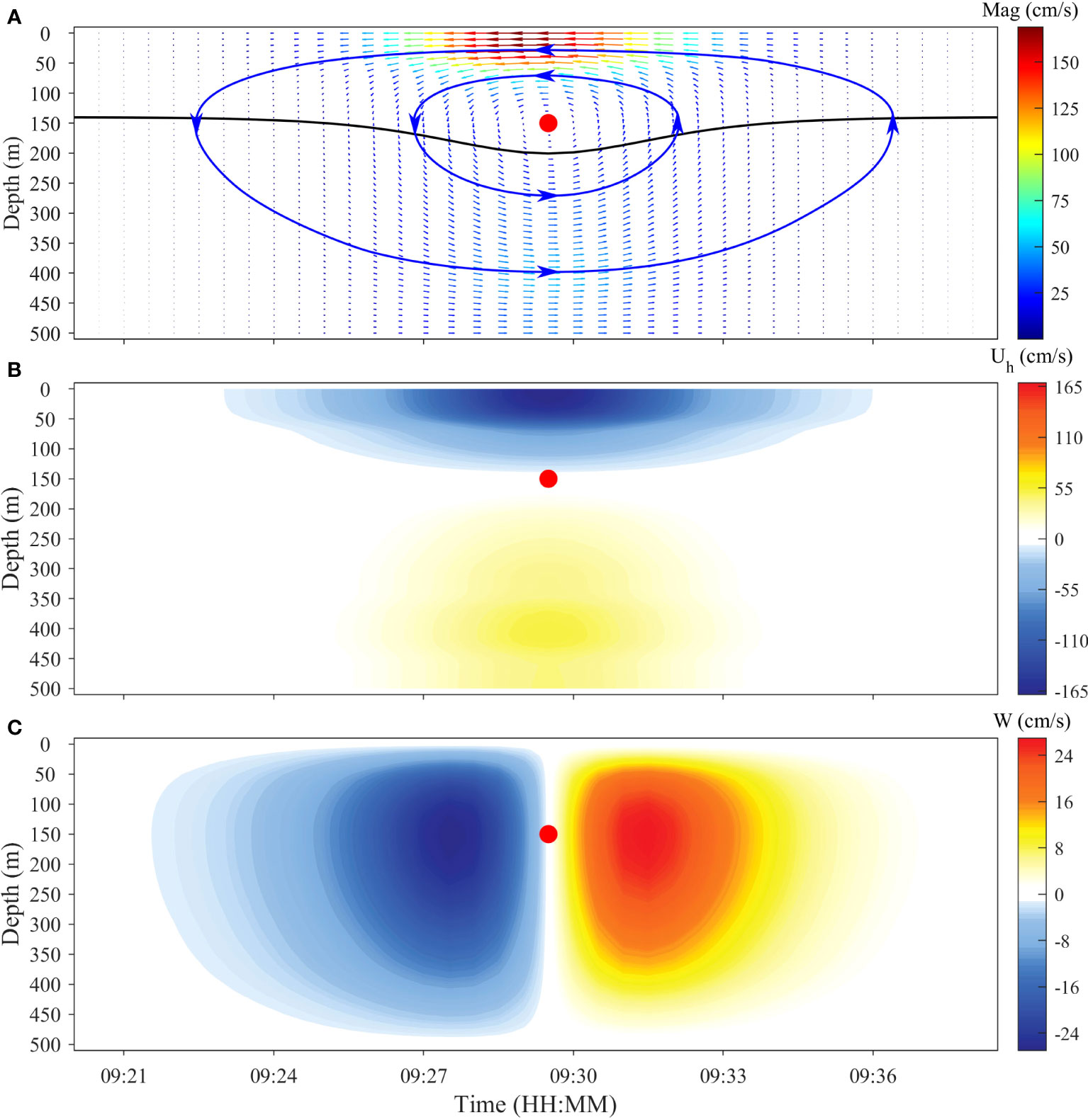
Figure 2 Vertical profiles of (A) velocity vectors, (B) horizontal velocity, and (C) vertical velocity field of mode-1 ISW simulated by the KdV theory. The black and blue curves in (A) represent the waveform of ISW with maximum amplitude and streamlines, respectively. The solid red dots in each subgraph represent the center of the ISW flow.

2.3 Identification of the ISW current center

The velocity field of the eddy is generally characterized by some typical features, such as minimum velocities in the proximity of the eddy center and tangential velocities that increase almost linearly with distance from the center before reaching a maximum value and then declining (Dickey et al., 2008; Nencioli et al., 2008). According to the characteristics of the eddy velocity field, Nencioli et al. (2010) developed an eddy detection algorithm based on the Vector Geometry (VG) method. This algorithm contained four constraints corresponding to the definition and features of the eddy velocity field. The grid point in the field for which all these four constraints are satisfied was detected as the eddy center (Dong et al., 2017).

The submersible mooring system was usually used for in-situ observation of the ISWs so that the instantaneous velocity field similar to the eddy cannot be obtained, and only the variations in velocity at each depth with time can be measured. In addition, due to the action of gravity and buoyancy of water particles in the ISW current, and the influence of boundary near the sea surface or seabed, the variational trends of the horizontal and vertical velocity vectors are not the same. Therefore, in this study, some improvements and additions to VG were incorporated based on the geometric characteristics of the ISW flow field mentioned in the last section. The algorithm identifies the ISW by determining the center of the ISW current, which must satisfy the following five constraints (which the constraints (A) and (B) are improved based on VG, and constraint (E) is the supplementary condition in this study):

(A) The vertical velocity component $w$ along the time direction of the ISW center has opposite numerical signs on either side of the center;

(B) The horizontal velocity component $u_h$ along the depth direction of the ISW center has opposite numerical signs on either side of the center;

(C) The grid point with minimum velocity in the selected area is approximately detected as the ISW center;

(D) Around the ISW center, the directions of rotation of the velocity vectors must be consistent, i.e., the directions of two neighboring velocity vectors have to lie within the same or two adjacent quadrants;

(E) The ratio of isotherm fluctuation to the depth of seawater before and after the ISW center is greater than 0.05.

The above constraints are ordered in progressive relationships and the central point of the ISW current can be determined by the limits of each constraint. It should be noted that two parameters used for detection were determined based on the above constraints, namely, $r_t$ representing the number of grid points along the time direction and $r_z$ representing the number of grid points along the depth direction (a grid point of $r_t$ and $r_z$ correspond to 30 s and 10 m, respectively in this study). These two parameters constituted a rectangular detection box with a size of $2r_t\times 2r_z$ for the detection and identification of each grid point in the entire velocity field of the ISW. The specific applications of these constraints are described in the next section.

2.4 Characteristic parameters of the ISW

The characteristic parameters (i.e., amplitude, duration and propagation direction) of the ISW are obtained by determining the start-stop time of the ISW. The vertical current velocity induced by the ISW is usually tens of centimeters per second, which distinguishes it from other marine phenomena. The variational curve of vertical velocity has the characteristics of Gaussian-like distribution, which is similar to the Mexican-Hat function. Therefore, by applying the wavelet transform to the vertical velocity sequence, the wavelet transform coefficient appears to have a local extremum at the jump point of the velocity sequence and can be used to determine the start-stop time of the ISW (Figure 3).

FIGURE 3

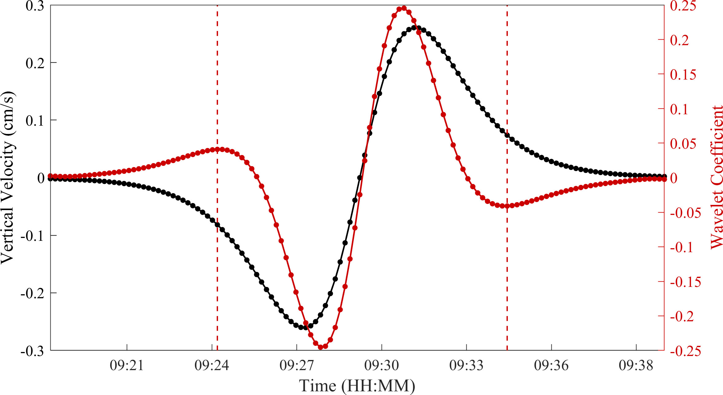
Figure 3 Variation cures of vertical current velocity (black curve) and wavelet transform coefficient (red curve) at the depth of 250 m in Figure 2C. The red dotted lines represent the start-stop time.

Based on the above methods, the automatic process to identify the center of ISW was developed as follows (Figure 4): Firstly, the vertical profile of the measured current $(u,v,w)$ was converted to the horizontal direction of ISW propagation ($\theta$ ). Since the remote sensing data highlighted that most of the ISWs in the west sea area of the Dongsha Islands propagated westward with the angle between 210° and 360° with an average of 301.7° (Wang et al., 2013), $\theta$ was set at 300° in this study. Secondly, the parameters $r_t$ and $r_z$ were initially determined and then the first four constraints were applied to detect all the grid points in the profile of the measured current. Further, the fifth constraint was applied after combining it with the temperature profile. The grid point in the profile satisfying all the five constraints was considered as the center of ISW current, thereby leading to the successful identification of the ISW. Finally, the start-stop time and duration of the ISW were determined by applying the wavelet transform to the vertical current velocity. The amplitude of the ISW was expressed as the maximum vertical displacement of the isotherm. The propagation direction of the ISW is the same as that of the upper horizontal velocities induced by the ISW (Liu et al., 2004).

FIGURE 4

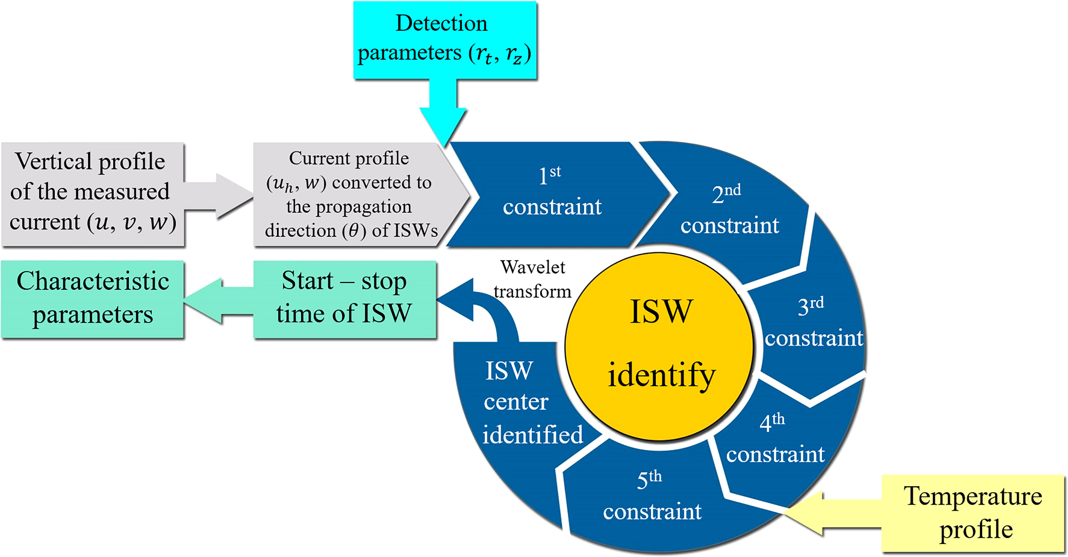
Figure 4 Flow chart for the automatic identification of the ISW.

3 Results and analysis

3.1 Identification of ISW in theoretical simulation

Figure 5 shows the process of identification of the central point of the ISW current (same as Figure 2A) simulated by the KdV theory, where the ISW flow field was represented by the velocity vector matrix. The first three constraints were applied to all the grid points (velocity vectors) in Figure 5A for detection. Firstly, the grid points in each row (at each depth) where the numerical signs of $w$ changed (i.e., zero-crossings) were determined. If $w$ has opposite numerical signs at the positions $\pm r_t$ away from these points in the horizontal direction (axis of time), then the grid points in the field that satisfied the first constraint were selected (red circles in Figure 5A). Secondly, if $u_h$ has opposite numerical signs at the positions $\pm r_z$ away from these selected points in the vertical direction (axis of depth), the grid points that satisfied the second constraint were selected (red circles in Figure 5B). Lastly, among the points that satisfied the first two constraints, the point with the minimum velocity in the detection range of $2r_t\times 2r_z$ centered on these points was considered to be the approximate center of the ISW current (red circle in Figure 5C), i.e., the point satisfying the first three constraints. Further, the fourth constraint was applied to check the velocity vectors around this point. The velocity vectors on the colored solid ($2r_t\times 2r_z$) and dotted ($r_t\times r_z$) rectangles are represented by arrows in Figure 5C. As shown in Figure 6, these velocity vectors are arranged counterclockwise from the upper left corner of the rectangles with the quadrants indicated. It can be observed that the velocity vectors rotate counterclockwise and the adjacent velocity vectors lie within the same or two adjacent quadrants, thus satisfying the fourth constraint. Therefore, the position of the red circle in Figure 5C was identified as the center of the ISW current and the ISW was detected successfully.

FIGURE 5

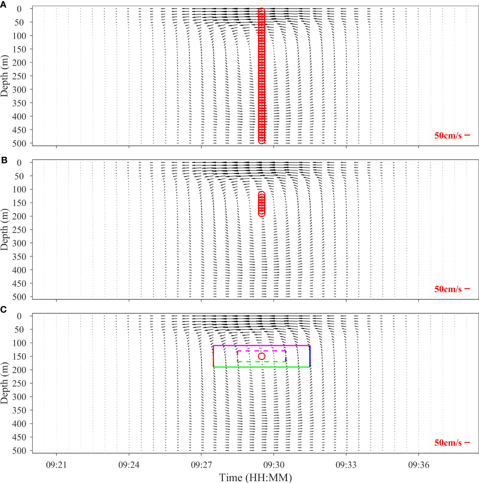
Figure 5 (A) First, (B) second, and (C) third constraints applied to the ISW current field simulated by the KdV theory. The red circles in each subgraph represent the grid points that satisfy the constraints. The colored solid and dotted rectangles in (C) represent the search scope, and the velocity vectors on the edges need to be further screened by applying the fourth constraint ($r_t=r_z=4$ ).

FIGURE 6

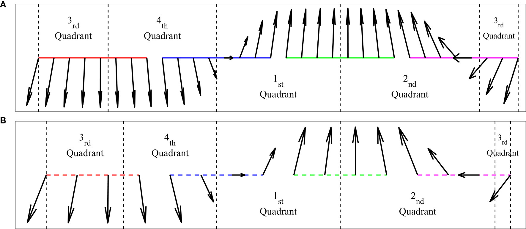
Figure 6 Velocity vector arrows on the colored (A) solid and (B) dotted rectangles in Figure 5C arranged counterclockwise from the upper left corner of the rectangle. The vector arrows between two adjacent black dashed lines are located in the same quadrant.

3.2 Identification of ISW in the mooring observation

Furthermore, the algorithm was applied to the observation data for verification. Figure 7A shows the ISW current with an amplitude of 60.58 m observed at mooring B on 4 August 2018. The flow field characteristics of the observed ISW were consistent with that simulated by the KdV theory (Figure 2A). Same as the last section, the first three constraints were applied to the velocity vector field (Figure 7A), and an approximate center (red circle in Figure 7C) of the ISW current that satisfied the first three constraints was determined. The fourth and fifth constraints (the ISW amplitude was expressed as the maximum vertical displacement of the isotherm) were applied for further screening of this approximate center (Figures 8, 9). Thus, the center of the ISW was identified successfully (white circle in Figure 9).

FIGURE 7

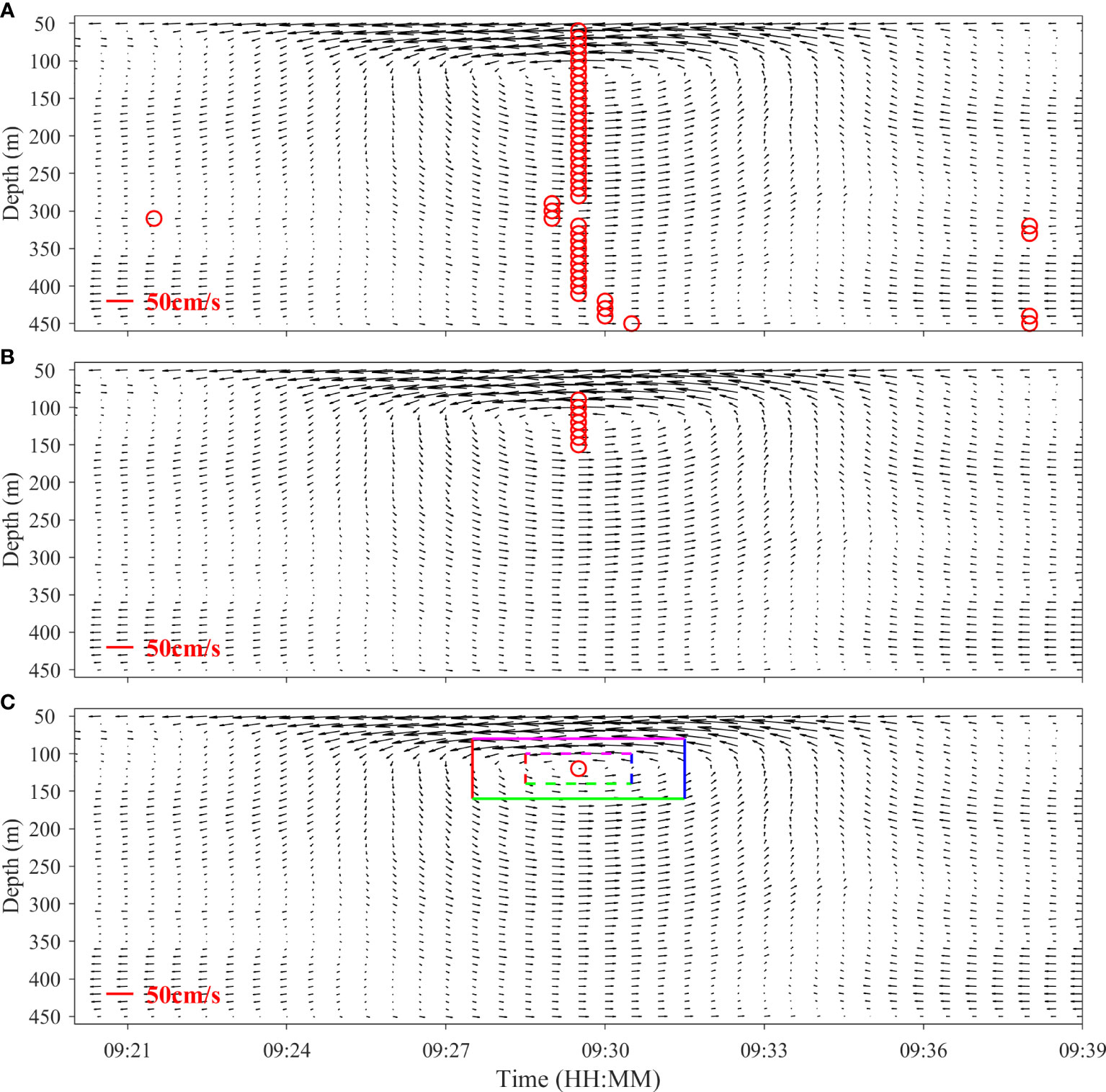
Figure 7 The (A) first, (B) second, and (C) third constraints applied to the measured ISW current field observed at mooring B on 4 August 2018. The red circles in each subgraph represent the grid points that satisfy the constraints. The length of the red line in the lower left corner of each subgraph indicates the velocity of 50 cm/s. The colored solid and dotted rectangles in (C) represent the search scope, and the velocity vectors on the edges need to be further screened by applying the fourth constraint ($r_t=r_z=4$).

FIGURE 8

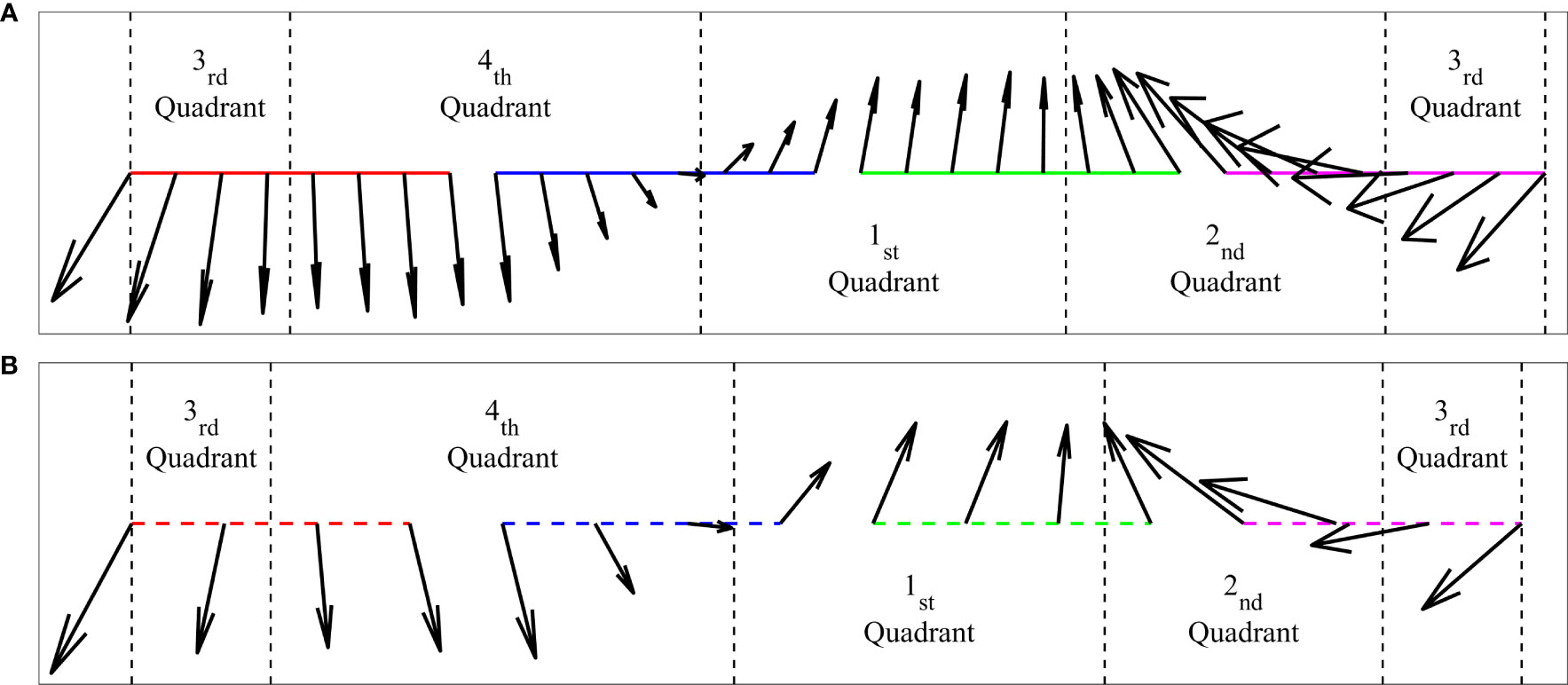
Figure 8 Velocity vector arrows on the colored (A) solid and (B) dotted boxes in Figure 7C arranged counterclockwise from the upper left corner of the rectangle. The vector arrows between two adjacent black dashed lines are located in the same quadrant.

FIGURE 9

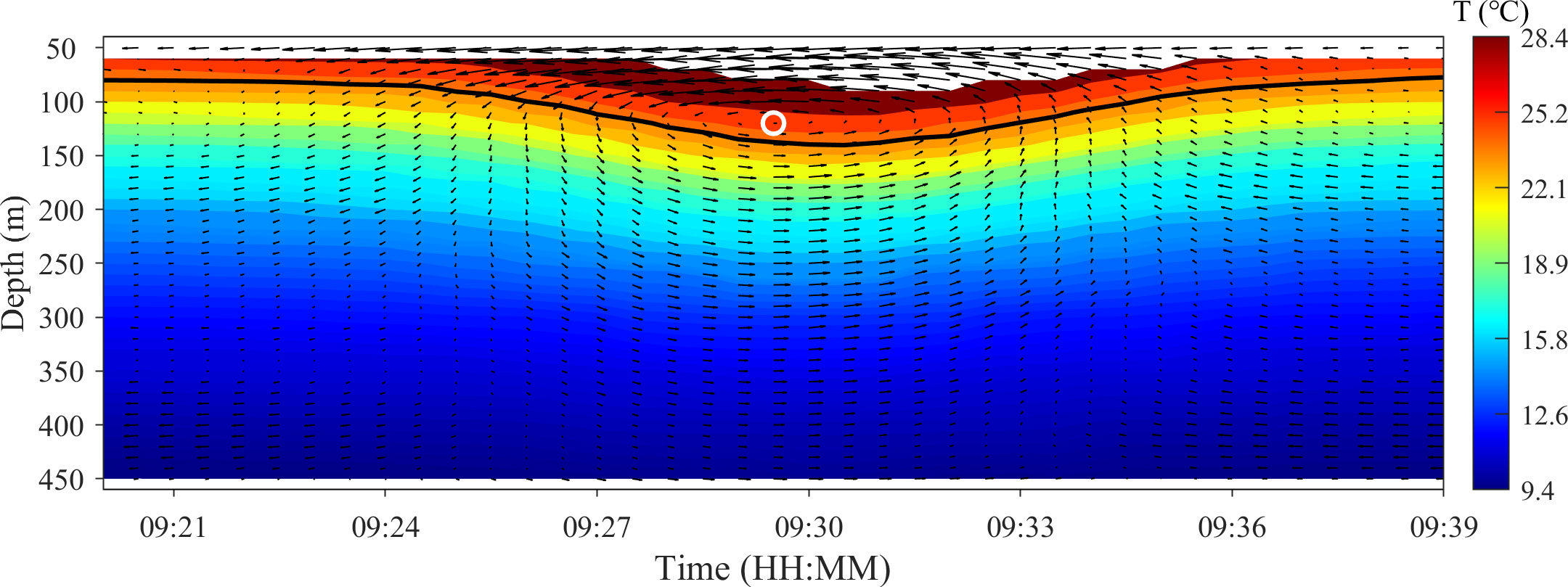
Figure 9 Vector arrows of the ISW current in Figure 7 and the profile of temperature oscillation during the occurrence of the ISW. The black curve represents the waveform with maximum amplitude. The white circle represents the grid points that satisfy all the constraints, corresponding to the red circle in Figure 7C.

Finally, the algorithm was applied to the observed ISW packet data for verification. Figure 10A shows the flow field of the ISW packet consisting of five single waves with amplitudes ranging from 39.37 m to 84.76 m observed at mooring B on 19 September 2018. Among the five single waves, the head wave (pioneer soliton) had the largest amplitude with the maximum velocity, while the amplitudes and velocities of the other four residual waves decreased successively. The characteristics of every single wave were the same as those in Figure 7A. Furthermore, the center identification method described previously was applied to the ISW packet (Figures 10A–D), and the centers of the five single waves were successfully identified (white circles in Figure 10E).

FIGURE 10

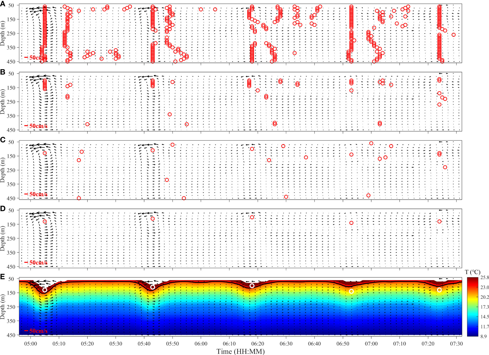
Figure 10 The (A) first, (B) second, (C) third, and (D) fourth constraints applied to the measured current field of the ISW packet observed at mooring B on 19 September 2018. The red circles in each subgraph represent the grid points that satisfy the constraints ($r_t=r_z=4$ ). (E) Vector arrows of the ISW current and the profile of temperature oscillation during the occurrence of the ISW packet. The black curve represents the waveforms with maximum amplitude. The white circles represent the grid points that satisfy all the constraints, corresponding to the red circles in (D).

3.3 Sensitivity analysis

Among the constraints considered for the automatic identification algorithm of the ISW, the selection of $r_t$ and $r_z$ directly affected the accuracy of ISW identification. Therefore, sensitivity analysis experiments were carried out for the determination of optimal parameter combinations. Firstly, two indicators were adopted to further evaluate the effectiveness of the algorithm, namely, true positive rate ($TPR$ ) and false negative rate ($FNR$ ) given by Equations 10 and 11, respectively.

$\begin{array}{ll}TPR=\frac{N_c}{N_i}& (10)\end{array}$

$\begin{array}{ll}FNR=\frac{N_m}{N_e}& (11)\end{array}$

where $N_i$ is the number of all centers identified by the algorithm, $N_c$ is the number of true ISWs identified by the algorithm, $N_e$ is the number of ISWs manually extracted, and $N_m$ is the number of ISWs not identified by the algorithm. The larger the $TPR$ and the smaller the $FNR$, the better the result of ISW identification. In addition, a parameter $ϵ$ was introduced for the determination of the optimal parameter combination, as expressed by Equation 12:

$\begin{array}{ll}ϵ=TPR\times (100\%-FNR)& (12)\end{array}$

Further, to improve $TPR$ and reduce $FNR$ as much as possible, the algorithm was applied to different combinations of $r_t$ and $r_z$ for the automatic identification of the measured flow fields during the observation period, and the results are shown in Figure 11.

FIGURE 11

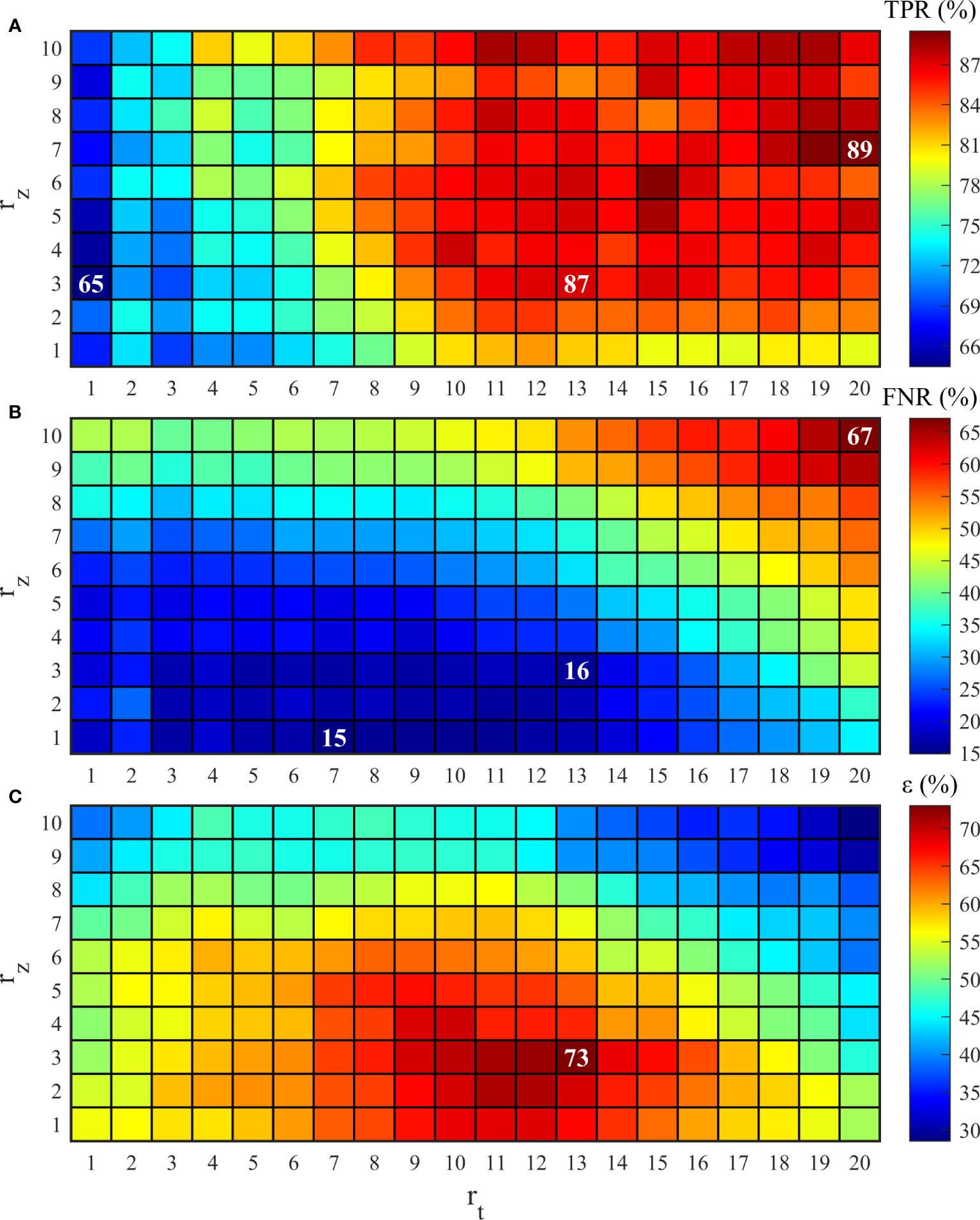
Figure 11 (A) $TPR$ , (B) $FNR$ and (C) $ϵ$ of the ISW identification algorithm at different $r_t$ and $r_z$.

It can be observed that for a given value of $r_z$ , a gradual decrease was observed in $TPR$ with the increase in $r_t$ (Figure 11A), whereas $FNR$ increased with the increase in both $r_t$ and $r_z$ (Figure 11B). $ϵ$ reached its maximum at $r_t=13$ and $r_z=3$ (Figure 11C). Finally, the optimal parameter combination of $r_t=13$ and $r_z=3$ was obtained through the sensitivity experiments, within the detection range of 13 min×60 m. The $TPR$ and $FNR$ of the ISW identification algorithm were 87.2% and 16.3%, respectively.

It is worth mentioning that whether in deep or shallow sea, the algorithm proposed in this paper is effective as long as the characteristic of the ISW current are obvious enough. While, the limitation of this study is that the identification of ISWs can be affected by the background current (such as tidal current, etc.). The elimination of the background current has always been a problem. In previous studies (Zhao et al., 2012; Li et al., 2015; Li et al., 2016; Chen et al., 2019), background current was mostly calculated by averaging the ADCP measurements during the pre- or post-ISW period. However, this method is not advisable in this study. In the previous studies, the ISW was observed and its arrival time was obtained directly, and in this study, the arrival time of the ISW was not known before the identification of the ISW. Therefore, the background current could not be calculated. Figure 12 shows the amplitudes and maximum background current velocities of the ISWs that were not detected by the algorithm. It can be observed that, for the ISW with a small amplitude, its geometric characteristics were not clear when the background current velocity was large, thereby leading to the low identification accuracy. The large ISWs can cause abrupt extreme shear currents which pose a serious threat to offshore structures (Wang et al., 2018). Therefore, more attention was paid to large ISWs in ocean engineering, and the identification results of the algorithm were found to be acceptable.

FIGURE 12

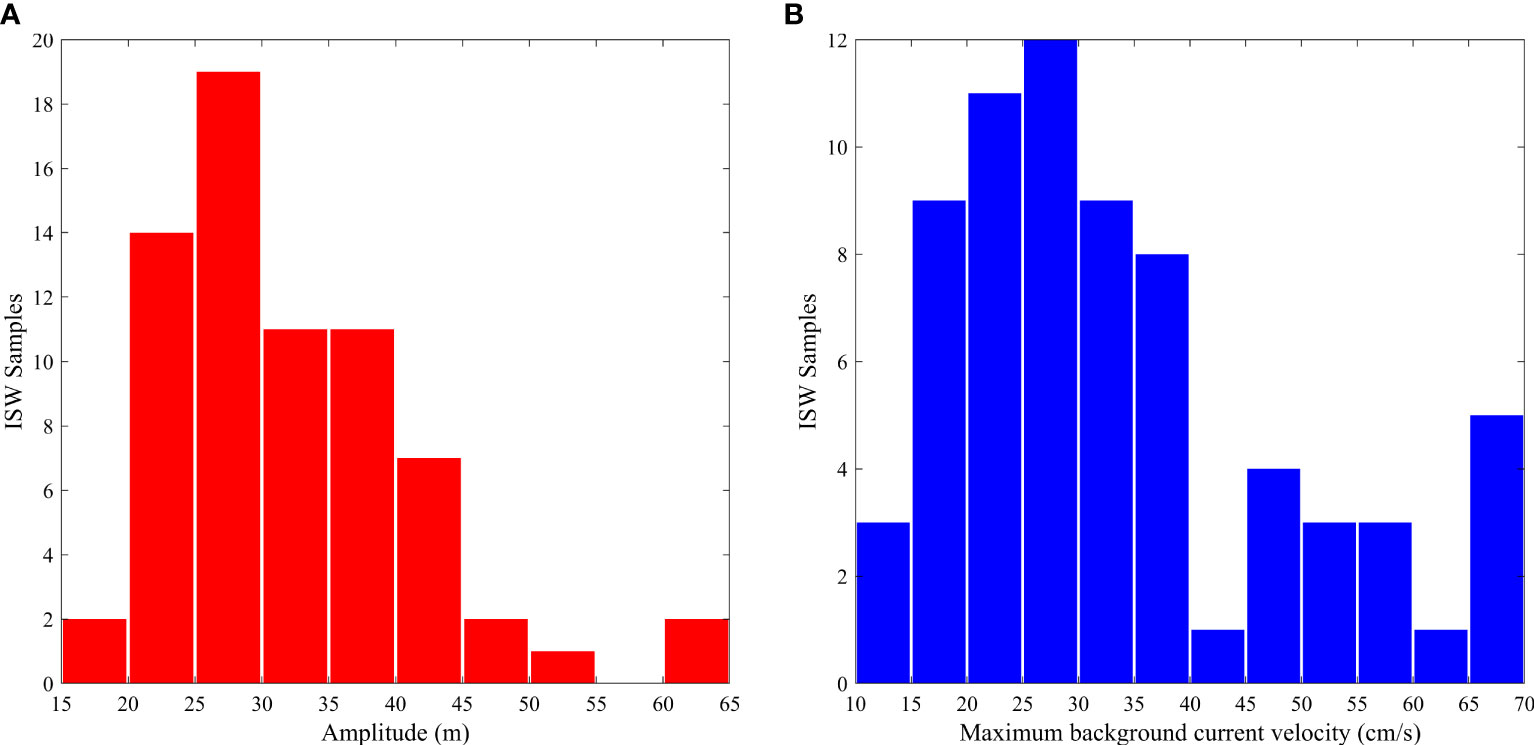
Figure 12 (A) Amplitudes and (B) maximum background current velocities of the ISWs that were not detected by the algorithm.

3.4 Statistics of characteristic parameters of ISWs

To further verify the reliability of the algorithm, the algorithm was applied to the characteristic parameters of the identified ISWs under the optimal parameter combination of $r_t=13$ and $r_z=3$ . As shown in Figure 13A, 69.03% of the ISW amplitudes were distributed between 20 and 60 m. The mean amplitude was 37.72 m with a maximum amplitude as large as 116.36 m and the amplitude of ISWs well fitted by the Rayleigh distribution. 78.14% of the ISW durations were distributed between 14 and 22 min. The mean duration was 17.44 min with a maximum duration as large as 29.37 min and the duration of ISWs well fitted by the Gaussian distribution (Figure 13B). In addition, the major propagation direction of ISWs was northwestward and the mean value of the maximum ISWs current velocities was 74.74 cm/s (Figure 14A). The statistical results obtained by the algorithm are in good agreement with the previous studies (Chen et al., 2019; Wang et al., 2022), implying the reliability of the algorithm.

FIGURE 13

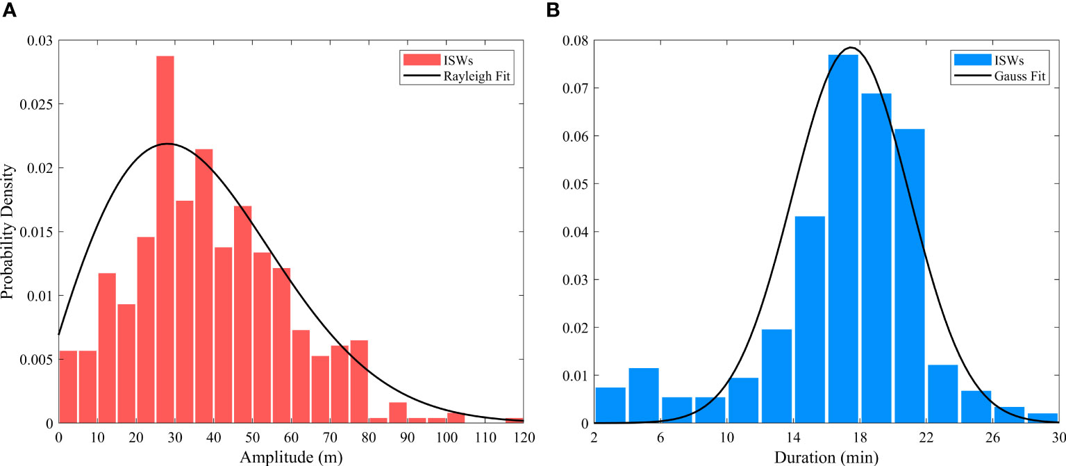
Figure 13 Probability density distributions of the (A) amplitudes and (B) duration of the ISWs identified by the algorithm.

FIGURE 14

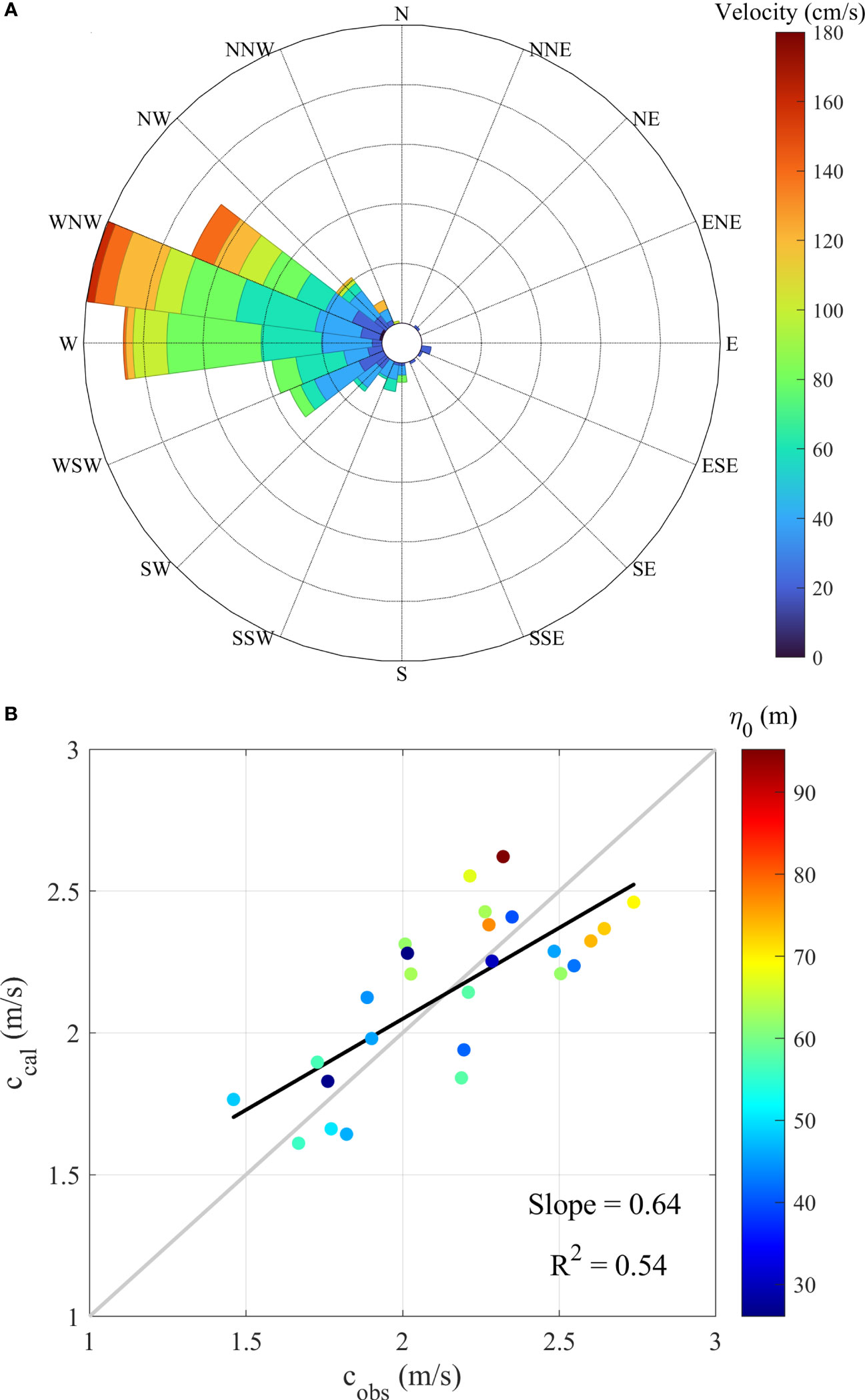
Figure 14 (A) Joint distribution of maximum current velocities and propagation directions of ISWs identified by the algorithm. (B) Comparison of measured ($c_{obs}$) propagation velocities of the ISWs with different amplitudes (${\eta }_0$) and those calculated by the algorithm ($c_{cal}$). R-squared ($R^2$) and slope of linear fit (black line) of the plots between $c_{obs}$ and $c_{cal}$ are represented.

Finally, the propagation velocity of ISW calculated by the algorithm ($c_{cal}$) was compared with the observation ($c_{obs}$). The KdV theory can well describe the propagation velocities of the ISWs with different amplitudes (Rong et al., 2023). Therefore, $c_{cal}$ can be calculated by Equation 4, and $c_{obs}$ can be approximated by the average velocity of the ISW propagating from mooring B to D, as expressed by Equation 13:

$\begin{array}{ll}{c}_{obs}=\frac{L_{BD}cos({\theta }_{BD}-{\theta }_{ISW})}{t_{BD}}& (13)\end{array}$

where $L_{BD}$ and $t_{BD}$ are the distance between the two moorings and propagation time, respectively. ${\theta }_{BD}$ is the angle of the line between two moorings clockwise from the north, and ${\theta }_{ISW}$ is the propagation direction of the ISW.

The statistical comparison results (Figure 14B) indicated that the average propagation velocity of ISWs was 2.14 m/s, which was generally consistent with the previous research results (Cai et al., 2014; Chen et al., 2019). The error of the propagation velocity was proportional to the amplitude of ISW, the maximum error was 0.35 m/s, and the average error was $\pm$ 0.20 m/s, which verified the reliability of the algorithm.

At present, the traditional identification algorithms usually identify the ISWs by calculating the vertical displacement of the isotherms, including the single isotherm (SI) method (Zhao and Alford, 2006; Cui et al., 2020) and the whole water column isotherm (WCI) method (Chen et al., 2019). For the SI method, a single isotherm cannot reflect the amplitudes of all ISWs. The WCI method is more efficient in identifying the ISWs for it considering the temperature signals of the entire water column. However, this method can only identify the ISWs under the condition that there are more than 6 isotherms (Gong et al., 2023). In addition, the above two methods can only calculate the amplitudes of the ISWs, but cannot accurately calculate other characteristic parameters, so it is difficult to apply these methods to the prediction of the ISWs in actual ocean. By comparison, the algorithm proposed in this study is more practical and can accurately obtain the initial parameters of the ISWs, so as to provide the guarantee for the subsequent early-warning of the ISWs.

4 Summary and discussion

In this study, an automatic identification algorithm of the ISWs was proposed for mooring observation. The algorithm includes five constraints based on the geometric characteristics of the ISW flow field, and the characteristic parameters of the ISWs can be obtained by the wavelet transform. When the algorithm was applied for detecting the velocity field of the ISW simulated by the KdV theory and that observed at the mooring, the results indicated that the algorithm accurately identified the center of the ISW and obtain relevant parameters.

In addition, the range of detection parameters $r_t$ and $r_z$ hould be set based on the constraints. These two parameters depend on the temporal and spatial resolutions and directly affect the accuracy of the ISW identification. Therefore, further sensitivity experiments were conducted. Based on a mooring deployed on the west slope of Dongsha Islands in the northern SCS, the algorithm was applied to the mooring dataset at different $r_t$ and $r_z$. Thus, the optimal parameter combination of $r_t=13$ and $r_z=3$ was obtained, and the $TPR$(True Positive Rate) and $FNR$ (False Negative Rate) of the ISW identification algorithm were determined to be 87.2% and 16.3%, respectively. It is worth noting that the algorithm achieves accurate identification of the ISW by extracting the vortex-like structure of the ISW flow field, thus the identification accuracy depends on the obviousness of the ISW current, and the ISW current is mainly interfered by local background current. For the ISW with small amplitude, its geometric characteristic was not clear when the background current velocity was large, thereby leading to the low identification accuracy. In addition, due to the impact range of the ISW is the total water depth (Xu, 1999; Chen et al., 2023), the algorithm requires nearly full-depth mooring data to obtain relatively complete structure of the ISW flow field.

Finally, the characteristic parameters of the ISW were calculated by applying the algorithm. The statistics indicated that the mean ISW amplitude and duration are 37.72 m and 17.44 min, respectively. The major propagation direction of ISWs was northwestward and the mean value of the maximum ISW current velocities was 74.74 cm/s. In addition, the error of propagation velocity calculated by the algorithm was less than 0.35 cm/s, which verified its credibility.

The algorithm can accurately and automatically identify the ISWs and calculate the characteristic parameters at the current position and time. Thus the ISWs can be automatically monitored in real-time. The identification results of the algorithm can be considered as the initial conditions in future studies, and the propagation model of the ISWs can be further established by numerical simulation (Lai et al., 2019) or artificial intelligence (Zhang and Li, 2022) for development of a local real-time accurate prediction system for the ISWs.

Data availability statement

The raw data supporting the conclusions of this article will be made available by the authors, without undue reservation.

Author contributions

LR: software, validation, formal analysis, writing – original draft and visualization. XX: conceptualization, resources, data curation, project administration and funding acquisition. LC: methodology, investigation, writing – review and editing and supervision. All authors contributed to the article and approved the submitted version.

Funding

This study was supported by the National Science and Technology Major Project (2016ZX05057015).

Acknowledgments

The monthly temperature and salinity data were provided by the National Oceanic and Atmospheric Administration (NOAA). We would like to thank the NOAA for supporting the data in this study. We also thank the reviewers for the constructive comments and detailed suggestions that improved the manuscript.

Conflict of interest

The authors declare that the research was conducted in the absence of any commercial or financial relationships that could be construed as a potential conflict of interest.

Publisher’s note

All claims expressed in this article are solely those of the authors and do not necessarily represent those of their affiliated organizations, or those of the publisher, the editors and the reviewers. Any product that may be evaluated in this article, or claim that may be made by its manufacturer, is not guaranteed or endorsed by the publisher.

Supplementary material

The Supplementary Material for this article can be found online at: https://www.frontiersin.org/articles/10.3389/fmars.2023.1147268/full#supplementary-material

References

Alpers W. (1985). Theory of radar imaging of internal waves. Nature 314 (6008), 245–247. doi: 10.1038/314245a0

CrossRef Full Text | Google Scholar

Apel J. R., Ostrovsky L. A., Stepanyants Y. A. (1995). Internal solitons in the ocean. J. Acoust. Soc Am. 98 (5), 2863–2864. doi: 10.1121/1.414338

PubMed Abstract | CrossRef Full Text | Google Scholar

Bole J. B., Ebbesmeyer C. C., Romea R. D. (1994). “Soliton currents in the South China Sea: measurements and theoretical modeling,” Paper presented at the Offshore Technology Conference, Houston, Texas. doi: 10.4043/7417-MS

CrossRef Full Text | Google Scholar

Cai S. (2015). Numerical model of internal solitary waves and its application in the South China Sea (Beijing: Ocean Press).

Google Scholar

Cai S., Long X., Gan Z. (2003). A method to estimate the forces exerted by internal solitons on cylindrical piles. Ocean Eng. 30 (5), 673–689. doi: 10.1016/S0029-8018(02)00038-0

CrossRef Full Text | Google Scholar

Cai S., Xie J., Xu J., Wang D., Chen Z., Deng X., et al. (2014). Monthly variation of some parameters about internal solitary waves in the South China Sea. Deep Sea Res. Part I: Oceanogr. Res. Papers 84, 73–85. doi: 10.1016/j.dsr.2013.10.008

CrossRef Full Text | Google Scholar

Chen L., Xiong X., Zheng Q., Rong L., Wang Y., Gong Q. (2023). Analysis of mooring-observed bottom current on the northern continental shelf of the South China Sea. Front. Mar. Sci. 10. doi: 10.3389/fmars.2023.1164790

CrossRef Full Text | Google Scholar

Chen L., Zheng Q., Xiong X., Yuan Y., Xie H., Guo Y., et al. (2019). Dynamic and statistical features of internal solitary waves on the continental slope in the northern South China Sea derived from mooring observations. J. Geophys. Res. Oceans 124 (6), 4078–4097. doi: 10.1029/2018JC014843

CrossRef Full Text | Google Scholar

Chiu C. S., Ramp S. R., Miller C. W., Lynch J. F., Duda T. F., Tang T. Y. (2004). Acoustic intensity fluctuations induced by South China Sea internal tides and solitons. IEEE J. Oceanic Eng. 29 (4), 1249–1263. doi: 10.1109/JOE.2004.834173

CrossRef Full Text | Google Scholar

Cui Z., Liang C., Lin F., Jin W., Ding T., Wang J. (2020). The observation and analysis of the internal solitary waves by mooring system in the Andaman Sea. J. Mar. Sci. 38 (4), 16–25. doi: 10.3969/j.issn.1001-909X.2020.04.002

CrossRef Full Text | Google Scholar

Dickey T. D., Nencioli F., Kuwahara V. S., Leonard C., Black W., Rii Y. M., et al. (2008). Physical and bio-optical observations of oceanic cyclones west of the island of Hawai'i. Deep Sea Res. Part II: Topical Stud. Oceanography 55 (10-13), 1195–1217. doi: 10.1016/j.dsr2.2008.01.006

CrossRef Full Text | Google Scholar

Dong C., Jiang X., Xu G., Ji J., Lin X., Sun W., et al. (2017). Automated eddy detection using geometric approach, eddy datasets and their application. Adv. Mar. Sci. 35 (4), 439–453. doi: 10.3969/j.issn.1671-6647.2017.04.001

CrossRef Full Text | Google Scholar

Dong J., Zhao W., Chen H., Meng Z., Shi X., Tian J. (2015). Asymmetry of internal waves and its effects on the ecological environment observed in the northern South China Sea. Deep Sea Res. Part I: Oceanogr. Res. Papers 98, 94–101. doi: 10.1016/j.dsr.2015.01.003

CrossRef Full Text | Google Scholar

Duda T. F., Lynch J. F., Irish J. D., Beardsley R. C., Ramp S. R., Chiu C. S., et al. (2004). Internal tide and nonlinear internal wave behavior at the continental slope in the northern South China Sea. IEEE J. Oceanic Eng. 29 (4), 1105–1130. doi: 10.1109/JOE.2004.836998

CrossRef Full Text | Google Scholar

Ebbesmeyer C. C., Coomes C. A., Hamilton R. C., Kurrus K. A., Sullivan T. C., Salem B. L., et al. (1991). New observations on internal waves (solitons) in the South China Sea using an acoustic Doppler current profiler. Mar. Technol. Soc. 91 Proc., 165–175.

Google Scholar

Gong Q., Chen L., Diao Y., Xiong X., Sun J., Lv X. (2023). On the identification of internal solitary waves from moored observations in the northern South China Sea. Sci. Rep. 13, 3133. doi: 10.1038/s41598-023-28565-5

PubMed Abstract | CrossRef Full Text | Google Scholar

Grimshaw R., Pelinovsky E., Talipova T., Kurkina O. (2010). Internal solitary waves: propagation, deformation and disintegration. Nonlinear Process. Geophys. 17, 633–649. doi: 10.5194/npg-17-633-2010

CrossRef Full Text | Google Scholar

Guo L. (2020). Research on detection and parameters extraction of marine internal waves in high resolution and wide swath SAR (Harbin, China: Harbin Institute of Technology).

Google Scholar

Holloway P. E., Pelinovsky E., Talipova T., Barnes B. (1997). A nonlinear model of internal tide transformation on the Australian North West Shelf. J. Phys. Oceanogr. 27 (6), 871–896. doi: 10.1175/1520-0485(1997)027<0871:ANMOIT>2.0.CO;2

CrossRef Full Text | Google Scholar

Hong D. B., Yang C. S., Ouchi K. (2015). Estimation of internal wave velocity in the shallow South China Sea using single and multiple satellite images. Remote Sens. Lett. 6 (6), 448–457. doi: 10.1080/2150704X.2015.1034884

CrossRef Full Text | Google Scholar

Korteweg D. J., De Vries G. (1895). On the change of form of long waves advancing in a rectangular canal, and on a new type of long stationary waves. London Edinburgh Dublin Philos. Magazine J. Sci. 39 (240), 422–443. doi: 10.1080/14786449508620739

CrossRef Full Text | Google Scholar

Lai Z., Jin G., Huang Y., Chen H., Shang X., Xiong X. (2019). The generation of nonlinear internal waves in the South China Sea: a three-dimensional, nonhydrostatic numerical study. J. Geophys. Res. Oceans 124 (12), 8949–8968. doi: 10.1029/2019JC015283

CrossRef Full Text | Google Scholar

Li L., Wang C., Grimshaw R. (2015). Observation of internal wave polarity conversion generated by a rising tide. Geophysical Res. Lett. 42 (10), 4007–4013. doi: 10.1002/2015GL063870

CrossRef Full Text | Google Scholar

Li Y., Wang C., Liang C., Li J., Liu W. (2016). A simple early warning method for large internal solitary waves in the northern South China Sea. Appl. Ocean Res. 61, 167–174. doi: 10.1016/j.apor.2016.11.002

CrossRef Full Text | Google Scholar

Liu A. K., Hsu M. K. (2004). Internal wave study in the South China Sea using synthetic aperture radar (SAR). Int. J. Remote Sens. 25 (7-8), 1261–1264. doi: 10.1080/01431160310001592148

CrossRef Full Text | Google Scholar

Liu A. K., Ramp S. R., Zhao Y., Tang T. Y. (2004). A case study of internal solitary wave propagation during ASIAEX 2001. IEEE J. Oceanic Eng. 29 (4), 1144–1156. doi: 10.1109/JOE.2004.841392

CrossRef Full Text | Google Scholar

Ma X., Yan J., Hou Y., Lin F., Zheng X. (2016). Footprints of obliquely incident internal solitary waves and internal tides near the shelf break in the northern South China Sea. J. Geophys. Res. Oceans 121 (12), 8706–8719. doi: 10.1002/2016JC012009

CrossRef Full Text | Google Scholar

Masunaga E., Fringer O. B., Yamazaki H., Amakasu K. (2016). Strong turbulent mixing induced by internal bores interacting with internal tide-driven vertically sheared flow. Geophys. Res. Lett. 43 (5), 2094–2101. doi: 10.1002/2016GL067812

CrossRef Full Text | Google Scholar

McPhee-Shaw E. (2006). Boundary-interior exchange: Reviewing the idea that internal-wave mixing enhances lateral dispersal near continental margins. Deep Sea Res. Part II: Topical Stud. Oceanography 53 (1-2), 42–59. doi: 10.1016/j.dsr2.2005.10.018

CrossRef Full Text | Google Scholar

Murphy L. M. (1986). Linear feature detection and enhancement in noisy images via the Radon transform. Pattern recognition Lett. 4 (4), 279–284. doi: 10.1016/0167-8655(86)90009-7

CrossRef Full Text | Google Scholar

Nencioli F., Dong C., Dickey T., Washburn L., McWilliams J. C. (2010). A vector geometry–based eddy detection algorithm and its application to a high-resolution numerical model product and high-frequency radar surface velocities in the Southern California Bight. J. atmospheric oceanic Technol. 27 (3), 564–579. doi: 10.1175/2009JTECHO725.1

CrossRef Full Text | Google Scholar

Nencioli F., Kuwahara V. S., Dickey T. D., Rii Y. M., Bidigare R. R. (2008). Physical dynamics and biological implications of a mesoscale eddy in the lee of Hawai'i: Cyclone Opal observations during E-Flux III. Deep Sea Res. Part II: Topical Stud. Oceanography 55 (10-13), 1252–1274. doi: 10.1016/j.dsr2.2008.02.003

CrossRef Full Text | Google Scholar

Osborne A. R., Burch T. L., Scarlet R. I. (1978). The influence of internal waves on deep-water drilling. J. Petroleum Technol. 30 (10), 1497–1504. doi: 10.2118/6913-PA

CrossRef Full Text | Google Scholar

Pelinovsky E., Slunyaev A., Polukhina O., Talipova T. (2007). “Internal solitary waves,” in Solitary waves in fluids. Ed. Grimshaw B. R. (Boston: WIT Press, Southampton), 85–110.

Google Scholar

Rivera-Rosario G. A., Diamessis P. J., Jenkins J. T. (2017). Bed failure induced by internal solitary waves. J. Geophys. Res. Oceans 122 (7), 5468–5485. doi: 10.1002/2017JC012935

CrossRef Full Text | Google Scholar

Rong L., Xiong X., Chen L. (2023). Assessment of KdV and EKdV theories for simulating internal solitary waves in the continental slope of the South China Sea. Continental Shelf Res. 256, 104944. doi: 10.1016/j.csr.2023.104944

CrossRef Full Text | Google Scholar

Tian Z., Jia Y., Chen J., Liu J., Zhang S., Ji C., et al. (2021a). Internal solitary waves induced deep-water nepheloid layers and seafloor geomorphic changes on the continental slope of the northern South China Sea. Phys. Fluids 33 (5), 053312. doi: 10.1063/5.0045124

CrossRef Full Text | Google Scholar

Tian Z., Jia Y., Du Q., Zhang S., Guo X., Tian W., et al. (2021b). Shearing stress of shoaling internal solitary waves over the slope. Ocean Eng. 241, 110046. doi: 10.1016/j.oceaneng.2021.110046

CrossRef Full Text | Google Scholar

Tian Z., Liu C., Ren Z., Guo X., Zhang M., Wang X., et al. (2022). Impact of seepage flow on sediment resuspension by internal solitary waves: parameterization and mechanism. J. Oceanology Limnology 41 (2), 1–14. doi: 10.1007/s00343-022-2001-9

CrossRef Full Text | Google Scholar

Tian Z., Liu H., Zhang S., Wu J., Tian J. (2023). Prediction of shear stress induced by shoaling internal solitary waves based on machine learning method. Mar. Georesources Geotechnplogy 41 (2), 221–232. doi: 10.1080/1064119X.2022.2136045

CrossRef Full Text | Google Scholar

Wang Y., Dai C., Chen Y. (2007). Physical and ecological processes of internal waves on an isolated reef ecosystem in the South China Sea. Geophys. Res. Lett. 34 (18), 312–321. doi: 10.1029/2007GL030658

CrossRef Full Text | Google Scholar

Wang J., Huang W., Yang J., Zhang H., Zheng G. (2013). Study of the propagation direction of the internal waves in the South China Sea using satellite images. Acta Oceanol. Sin. 32 (5), 42–50. doi: 10.1007/s13131-013-0312-6

CrossRef Full Text | Google Scholar

Wang H., Ju X., Sun J., Yu L. (2022). Observation and analysis of the first mode internal solitary wave in the continental slope of the northern South China Sea in late spring. Adv. Mar. Sci. 40 (3), 399–407. doi: 10.12362/j.issn.1671-6647.20210707001

CrossRef Full Text | Google Scholar

Wang X., Zhou J., Wang Z., You Y. (2018). A numerical and experimental study of internal solitary wave loads on semi-submersible platforms. Ocean Eng. 150, 298–308. doi: 10.1016/j.oceaneng.2017.12.042

CrossRef Full Text | Google Scholar

Wu F., Yang Y., Xiong X., Chen L., Gong Q. (2022). Mechanism of internal solitary waves generated by the resonance of same-scale terrain and background current. Adv. Mar. Sci. 40 (2), 197–208. doi: 10.12362/j.issn.1671-6647.2022.02.004

CrossRef Full Text | Google Scholar

Xu Z. (1999). Dynamics of ocean internal waves (Beijing: Science Press).

Google Scholar

Yang J., Zhou C., Huang W., Xu M. (2000). Study on extracting internal wave parameter of SAR images. Remote Sens. Technol. Appl. 15 (1), 6–9. doi: 10.11873/j.issn.1004-0323.2000.1.6

CrossRef Full Text | Google Scholar

Yuan Q., Mao J., Feng L., Fan Z. (2013). Effect of internal soliton in South China Sea on offshore installation operation and its prevention. Petroleum Eng. Construction 39 (6), 27–30. doi: 10.3969/j.issn.l001-2206.2013.06.006

CrossRef Full Text | Google Scholar

Zhang X., Li X. (2022). Satellite data-driven and knowledge-informed machine learning model for estimating global internal solitary wave speed. Remote Sens. Environ. 283, 113328. doi: 10.1016/j.rse.2022.113328

CrossRef Full Text | Google Scholar

Zhao Z. (2004). A study of nonlinear internal waves in the northeastern South China Sea, Ph.D. dissertation (Newark: Univ. of Del.), 188.

Google Scholar

Zhao Z., Alford M. (2006). Source and propagation of internal solitary waves in the northeastern South China Sea. J. Geophys. Res. Oceans 111 (C11). doi: 10.1029/2006JC003644

CrossRef Full Text | Google Scholar

Zhao W., Huang X., Tian J. (2012). A new method to estimate phase speed and vertical velocity of internal solitary waves in the South China Sea. J. oceanography 68 (5), 761–769. doi: 10.1007/s10872-012-0132-x

CrossRef Full Text | Google Scholar