A meta-deep-learning framework for spatio-temporal underwater SSP inversion

Sound speed distribution, represented by a sound speed profile (SSP), is of great significance because the nonuniform distribution of sound speed will cause signal propagation path bending with Snell effect, which brings difficulties in precise underwater localization such as emergency rescue. Compared with conventional SSP measurement methods via the conductivity-temperature-depth (CTD) or sound-velocity profiler (SVP), SSP inversion methods leveraging measured sound field information have better real-time performance, such as matched field process (MFP), compressed sensing (CS) and artificial neural networks (ANN). Due to the difficulty in measuring empirical SSP data, these methods face with over-fitting problem in few-shot learning that decreases the inversion accuracy. To rapidly obtain accurate SSP, we propose a task-driven meta-deep-learning (TDML) framework for spatio-temporal SSP inversion. The common features of SSPs are learned through multiple base learners to accelerate the convergence of the model on new tasks, and the model’s sensitivity to the change of sound field data is enhanced via meta training, so as to weaken the over-fitting effect and improve the inversion accuracy. Experiment results show that fast and accurate SSP inversion can be achieved by the proposed TDML method.

1 Introduction

Underwater acoustic wave has become the most popular signal carrier in underwater wireless sensor networks (UWSNs) because of its smaller attenuation and better long-distance propagation performance compared with radio or optical signal by Erol-Kantarci et al. (2011). However, unlike terrestrial radio, underwater sound speed has significant spatio-temporal variability due to the influence of temperature, salinity, pressure by Jensen et al. (2011). This variability will lead to significant Snell effects, which is reflected in the bending of signal propagation path. The bending path brings difficulties for accurate sonar ranging according to Dinn et al. (1995) and localization according to Isik and Akan (2009); Carroll et al. (2014); Liu et al. (2015); Wu and Xu (2017) in underwater applications such as target detection and rescue. Nevertheless, if the sound speed distribution is obtained, the signal propagation trajectory can be estimated for correcting ranging and positioning errors, which is of great significance for localization applications.

The sound speed distribution of a certain region is usually represented by a sound speed profile (SSP), which is intuitively expressed as a function of sound speed with depth. During the past decades, SSP inversion methods have been widely adopted in underwater wireless sensor networks for estimating sound speed distribution by leveraging sound field information such as time of arrival (TOA) and received signal strength indication (RSSI). The research of novel SSP inversion methods is very promising because they are more automatic and less labor-time-consuming than direct measurement of sound speed by sound velocity profiler (SVP) or conductivity-temperature-depth (CTD) systems refer to Zhang et al. (2015); Huang et al. (2018).

The SSP inversion is a difficult work because the classical ray tracing theory by Munk and Wunsch (1979) and normal mode theory by Munk and Wunsch (1983); Shang (1989) only establish the one-way mapping from ocean environmental information to sound field information, while to the best of our knowledge, there has been no empirical formula for the reverse mapping. Representative works of SSP inversion includes matching field processing (MFP) by Tolstoy et al. (1991), compressed sensing (CS) by Choo and Seong (2018); Li et al. (2019) and artificial neural networks (ANN) by Stephan et al. (1995); Huang et al. (2018). With the same degree of inversion accuracy when there are enough training data, the ANN outperforms MFP and CS in real-time performance due to the fact that after ANN converges, the SSP can be obtained through only once forward propagation by feeding measured sound field information, while iterative processes are ineluctable in MFP and CS based methods for searching the coefficients of principal components decomposed by the empirical orthogonal function (EOF).

For learning-based SSP inversion methods such as ANN, two conditions need to be satisfied: 1) training data and testing data should be taken from a same domain that is independent and identical distribution (i.i.d.) refer to Weiss et al. (2016); 2) there should be enough training data to avoid over-fitting problem. However, these two conditions are hard to be met at the same time because of two reasons. First, there are obvious spatio-temporal differences in the distribution and shape of SSPs as shown in Figures 1, 2, so SSPs sampled in different regions and time periods can not be used together as training data for a certain task. Second, due to the high labor and economic cost in measuring SSPs through SVP or CTD systems, SSPs are collected non-uniformly in different regions and time periods, leading to insufficient training SSPs in the spatio-temporal intervals that those tasks belong to. When training the learning model on a small dataset, which is called few-shot learning, there would be over-fitting problem (weak generalization performance), so that the inversion accuracy can not be guaranteed.

FIGURE 1

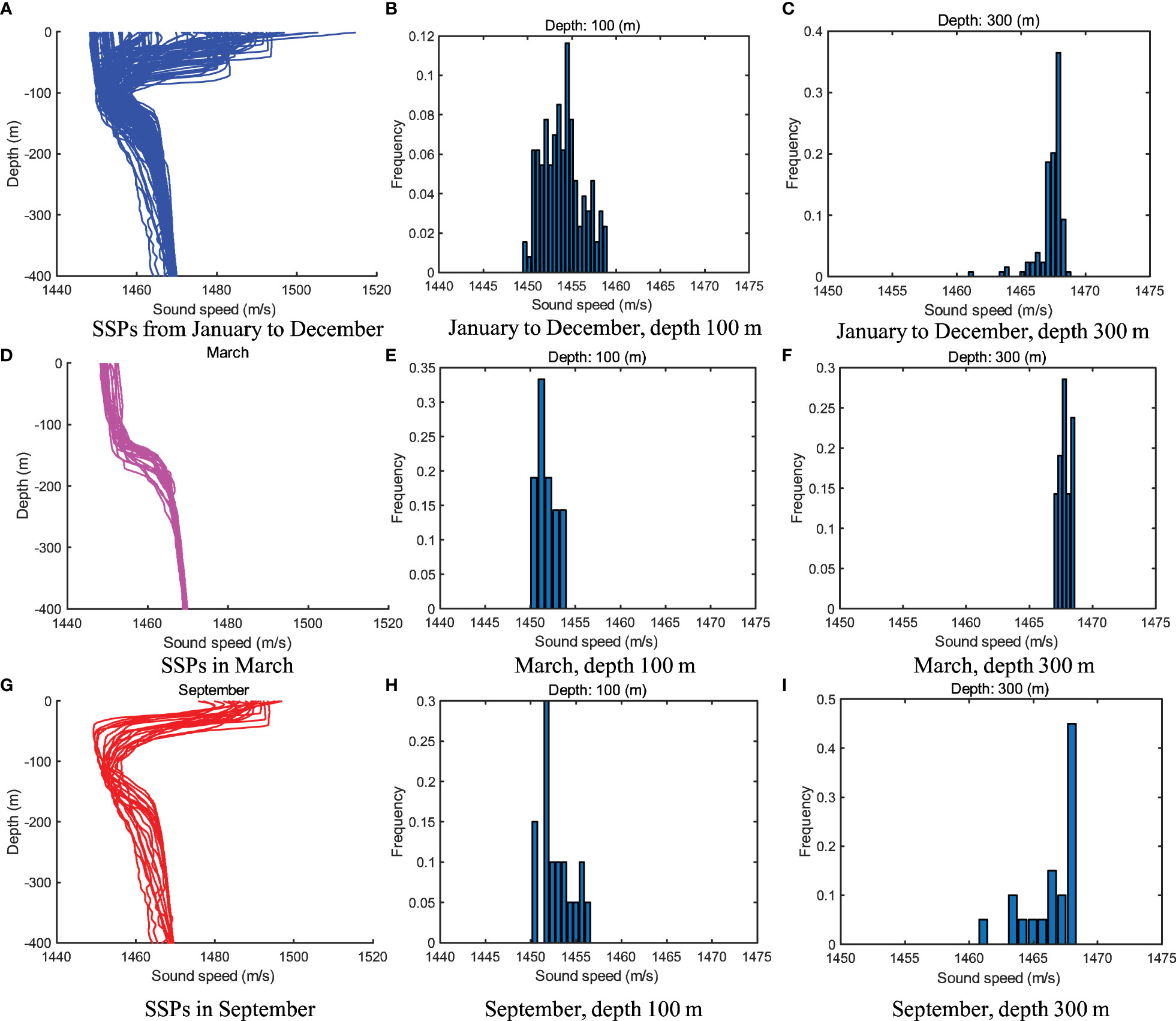
Figure 1 Historical SSPs sampled in different months from 40–50°C N and 150–160°C E of the North Pacific.

FIGURE 2

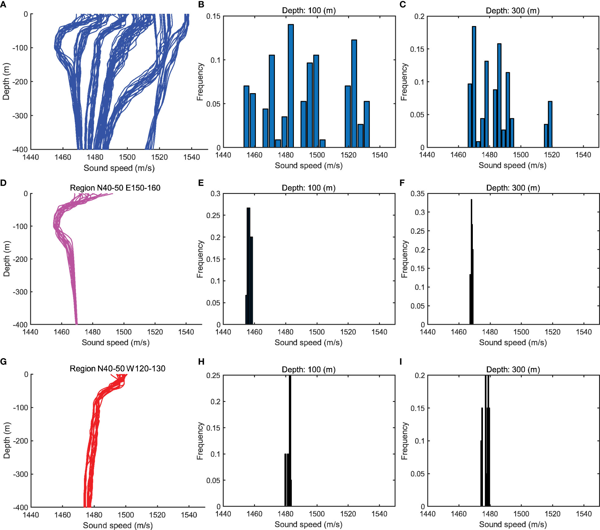
Figure 2 Historical SSPs sampled from different regions of the North Pacific Ocean in June (including historical periods).

For accurately estimating the sound speed distribution in a random ocean area, there are still two important problems to be solved: how to maintain good generalization ability of the inversion model especially in few-shot learning situations, and how to select appropriate reference SSPs for an inversion task to satisfy the i.i.d. condition without knowing the actual sound-speed distribution of the task. Many approaches have been proposed to deal with the overfitting problem, such as regularization by Goodfellow et al. (2016), training dataset expanding with generative adversarial networks by Jin et al. (2020), and meta-learning approach by Finn et al. (2017). Regularization establishes a way to limit the model scale by narrowing down the values of weight parameters (L2 norm) or making the model parameters sparse (L1 norm). By this way, the ability of fitting complex relationships of the model is weaken so that overfitting problem could be reduced. Training dataset expanding aims to enrich the training dataset that could represent the whole situation of target domain, however, if the original training data concentrates on a small region, the expanded training dataset will not be uniformly distributed in the target domain, thus the model is still prone to be overfitting. Although training dataset expanding could be achieved artificially to balance the distribution of training data, it usually needs a heavy workload.

Meta-learning (ML) is a newly emerging machine learning method that is very suitable for few-shot learning by Vanschoren (2018); Hospedales et al. (2020). Though ML, a learning model gains experience over multiple learning episodes that covering a distribution of related tasks, and uses the experience to improve its future learning performance for a designated task. The ‘learning to learn’ feature of ML could lead to a variety of benefits such as data and computing efficiency. Currently, many ML frameworks and algorithms have been established in typical fields such as classification by Snell et al. (2017), object detection by Pérez-Rúa et al. (2020) in computer vision, exploration policies by Alet et al. (2020) in robot control, domain adaptation by Cobbe et al. (2019), hyper–parameter optimization by Finn et al. (2017), neural architecture search summarized by Elsken et al. (2019), etc. The model-agnostic meta-learning (MAML) for fast adaptation of deep networks proposed by Finn et al. (2017) establishes a fast training method for deep learning models on few-shot learning tasks, which becomes almost the most famous work of hyper–parameter optimization. Though MAML provides an idea of model optimization, it has inspired the solution of few-shot learning problems in many fields such as meta-reinforcement learning framework by Alet et al. (2020) for exploration issues. Due to the fact that historical SSPs are usually not accompanied by sound field data, the labeled data composed of sound field data and SSPs need to be constructed through ray theory, resulting in the inability to directly adopt meta learning frameworks from other fields into construction of underwater sound speed field. Therefore, it is necessary to establish a more applicable meta learning SSP inversion framework based on the practical problems in underwater SSP inversion.

In this paper, we propose a meta-deep-learning framework for few-shot spatio-temporal SSP inversion named as task-driven meta-learning (TDML), which provides a training strategy that is suitable for multiple types of few-shot dataset learning. The core idea of TDML is to learn the common feature of different kinds of SSPs via a series of base learners, which forms a set of initialization parameters of the task learner. By this means, the convergence rate of the model could be accelerated and the sensibility to the input data could be retained, so that the model will not be over trained on few-shot task samples. The ability of fitting complex relationship or the training dataset is not changed by meta-learning itself, and it could be combined with regularization or training dataset expanding for solving overfitting issues in different applications. To guarantee that the distributions of reference SSPs and the inversion task meet the i.i.d. condition, all historical SSPs are first classified into different clusters by a proposed Pearson-correlation-based SSP local density clustering (PC-SLDC) algorithm, then the cluster which the task belongs to is decided by a proposed spatio-temporal-information-based K-nearest neighbor (STI-KNN) mapping algorithm. The contribution of this paper is summarized as follows:

● To accurately obtain sound-speed distribution in a random ocean area under few-shot learning situations, we propose a task-driven meta-deep-learning framework for spatio-temporal SSP inversion.

● To reduce negative transfer effect and deal with the over-fitting problem, we propose a task-driven meta-deep-learning SSP inversion algorithm, in which the updating rate of neuron connection weights could be dynamically adjusted and the convergence of inversion model could be accelerated.

● To satisfy the i.i.d. condition and select reference SSPs that possibly has the most similar distribution to the inversion task, we first propose a Pearson-correlation-based SSP local density clustering algorithm for historical SSPs clustering, then propose a spatio-temporal-information-based K-nearest neighbor algorithm for mapping the inversion task to a proper cluster leveraging the spatio-temporal information.

The rest of this paper is organized as follows. In Sec. 2, we briefly review related works about SSP inversion and few-shot learning. In Sec. 3, the source of input data during training and inversion phase is provided. In Sec. 4, we first propose a TDML framework for spatio-temporal SSP inversion, then present an SSP clustering algorithm and task mapping algorithm to find proper reference SSPs for a specified inversion task. Simulation results are discussed in Sec. 5, and conclusions are given in Sec. 6.

2 Related works

2.1 Underwater SSP inversion

MFP, CS and ANN are three classical SSP inversion methods. In Tolstoy et al. (1991), the MFP technique is first introduced in SSP inversion with four steps: empirical orthogonal decomposition, candidate SSPs generation, simulated sound field calculation and sound field matching, the candidate SSP corresponding to the optimal matching sound field will be recorded as the final inversion result. Instead of reverse mapping from sound field information to sound speed distribution, the purpose of MFP is to find matching principal component coefficients. However, the high time complexity debase the real-time performance of MFP. In Li and Zhang (2010), the coefficient searching space was reduced first, then a traversal method was used to find the optimal solution, while in Li et al. (2015) a parallel grid searching algorithm was proposed to reduce the time consumption. However, the searching accuracy depends on the scanning step, so that the time overhead increases as the accuracy of SSP inversion improves. Heuristic optimization algorithms were introduced in Zhang (2005); Tang and Yang (2006); Zhang et al. (2012); Sun et al. (2016); Zheng and Huang (2017) to speed up the searching process of the optimal EOF coefficients, such as the simulated annealing algorithm in Zhang (2005), genetic algorithm in Tang and Yang (2006); Sun et al. (2016), and particle swarm optimization (PSO) algorithm in Zhang et al. (2012); Zheng and Huang (2017). However, to get the optimal result with a high probability, multiple iterations are necessary in these heuristic algorithms. Consequently, the time overhead of SSP inversion can not be reduced to a desired level.

In Li et al. (2019), a mapping relationship is established as a dictionary to describe the effect of small perturbation of principal component coefficients on the change of sound field data. Because the principal component coefficients can be solved directly by the dictionary and sound field data with a few iterations of the least-squares calculation, it can achieve better real-time performance than MFP. Nevertheless, the first-order Taylor expansion approximation for the nonlinear mapping relationship is adopted in the design of the dictionary, so the inversion accuracy is sacrificed to some extent.

Recently, Bianco et al. (2019) presented a detailed review of machine learning applications in the field of acoustic, showing that machine learning technologies have become very promising in ocean parameter estimation, such as seafloor characterization by Michalopoulou et al. (1993), range estimation by Komen et al. (2020), geoacoustic inversion by Piccolo et al. (2019), and SSP inversion by Bianco and Gerstoft (2017). A dictionary learning method is proposed in Bianco and Gerstoft (2017) for SSP inversion that can better explain sound speed variability with fewer coefficients compared with classical EOF decomposition, however, it still requires a lot of time for searching the related dictionary elements and coefficients.

Inspired by the ability of deep neural networks to fit nonlinear functions, we have proposed an ANN-based SSP inversion method in our previous works (Huang et al., 2018; Huang et al., 2021). Through off-line training, the ANN is able to learn the mapping relationship from signal propagation time to sound speed distribution; and during the inversion stage, the SSP can be estimated via once forward propagation by feeding the measured signal propagation time into the SSP inversion model, so the time overhead can be reduced. With enough training data, the ANN can hold a good inversion accuracy while significantly outperforms the MFP and CS in time overhead performance during the inversion stage, which indicates that the deep neural networks are very promising in the SSP inversion fields. However, due to the difficulty of SSP measurement and spatial-temporal distribution of SSP, the neural network model needs to be trained on small dataset in some cases, which is prone to be over-fitting. Therefore, how to deal with the over-fitting problem in few-shot learning is well worth studying.

2.2 Few-shot learning

Conventional deep neural networks are trained from scratch for a given task with lots of training samples. However, in some fields such as SSP inversion, historical data is scarce because of the difficulty in measuring SSPs by CTD or SVP systems, so the model should be able to learn the distribution features of data with only a small amount of samples, which is commonly known as few-shot learning. In this case, the conventional deep neural network will easily fall into over-fitting problem.

To solve the over-fitting problem in few-shot learning, some studies have been done recently as surveyed in Vanschoren (2018); Hospedales et al. (2020). Aiming at few-shot learning on specific tasks, multi-task learning jointly learns several related tasks, and benefits from the effect regularization due to parameter sharing refer to Rich (1997); Yang and Hospedales (2016). Transfer learning (TL) has been developed for few-shot learning in the past decade as surveyed in Weiss et al. (2016); Pan and Yang (2010). TL uses past experience of a source task to improve learning on a new task by transferring the model’s parameter prior in Chang et al. (2018) or the feature extractor from the solution of a previous task in Yosinski et al. (2014). Because the TL model is first trained on a specific task, features of the task are memorized in the model, which would affect the learning rate and accuracy for a new task.

Recently, ML surveyed by Vanschoren (2018); Hospedales et al. (2020) has become a promising method for few-shot learning. Different from MTL and TL, a meta-objective is usually defined in ML to evaluate how well the base learner performs when helping to learn a new task. In Ravi and Larochelle (2017), a long short-term memory meta-learner is used to learn an update rule for training a neural network learner. During the training phase, the base learner provides the current gradient and loss to the meta learner, which then update the model parameters. In Finn et al. (2017), a model-agnostic meta-learning algorithm is proposed to learn a model parameter initialization which achieves better generalization performance to similar tasks. The Hessian matrix is illustrated in Finn et al. (2017) for gradient descent, which enhance the sensitivity of the model to the input data. The work of Nichol et al. (2018) further improves the learning rate of model on a new task by executing stochastic gradient decent for several iterations.

The concept of ML would be suitable for dealing with the over-fitting problem of underwater sound speed inversion with only a few reference samples. However, the negative transfer effect caused by training with different kinds of SSPs still needs to be solved so as to improve the inversion accuracy.

3 Preliminary

The SSP inversion is to establish the mapping from signal propagation time to the sound speed distribution. For clearly illustrating the inversion model, it is important to know more about the source of input data. In this section, we will present the signal propagation time measurement method for SSP inversion, and derive the simulated signal propagation time by ray tracing theory corresponding to each historical SSP for training inversion model.

3.1 Signal propagation time measurement

For SSP inversion, accelerating the measurement of signal propagation time is of great important to improve the real-time performance. Thus, the autonomous underwater vehicle (AUV) assisted signal propagation measurement system proposed in our previous work Huang et al. (2021) is adopted in this paper, which has the advantages of stability and mobility compared with traditional ship-towed or seafloor fixed arrays in Zhang et al. (2015); Choo and Seong (2018); Li and Zhang (2010); Li et al. (2015); Zhang (2005); Tang and Yang (2006); Zhang et al. (2012); Zheng and Huang (2017); Zhang (2013).

The AUVs are able to suspend in the water. One AUV sailing at the bottom of the ocean act as the source node to start the measurement process, the other three AUVs are receivers that sail approximately in the same vertical plane with the bottom AUV and keep a fixed horizontal distance $\text{Δ}{\pi }_h$ from each other. During once time measurement, the signal travels a round trip, then the clock asynchronization error can be reduced via the bidirectional TOA technology. The idea of virtual anchoring is introduced to increase the amount of measured time data. After one turn of communication, the three AUVs move forward with the distance $\frac{\Delta {\pi }_h}{\Pi }$ and start a new turn of measurement. After moving $\text{Π}-1$ times, a signal propagation time sequence containing $3*\text{Π}$ items can be obtained as the measurement result.

3.2 Signal propagation time simulation

The learning model of SSP inversion is usually trained offline, so the required input signal propagation time can not be measured at the model training stage. Therefore, the classical ray tracing theory is introduced to provide signal propagation time information as input data corresponding to a given SSP for inversion model training.

Assume the preset horizontal distance series of the AUV system is $\text{Π}=[{\pi }^1,{\pi }^2,\dots ,{\pi }^m],m=1,2,\dots ,3\text{Π}$ that forms totally $M=3\text{Π}$ transceiver pairs, then for a given SSP $S={[(s^1,1),\dots ,(s^d,d)]}^T$, the relation between $\text{Π}$ and $S$ can be expressed according to our previous derivation Huang et al. (2021) as:

$\begin{array}{ll}\begin{array}{ll}{\pi }^m\hfill & =\frac{{}_s^1}{cos{\vartheta }^1{,}^m}{\displaystyle \sum _{d=1}^{D-1}}\left|\frac{\Delta z_d}{s^{d+1}-s^d}(\sqrt{{\Upsilon }_d^m}-\sqrt{{\Upsilon }_{d+1}^m})\right|,\hfill \\ {\Upsilon }_d^m\hfill & =1-{\left(\frac{cos {\vartheta }^1{,}^m}{s^1}\right)}^2{(s^d)}^2,\hfill \end{array}& (1)\end{array}$

where $D$ is the total depth of the SSP, ${\vartheta }^1{,}^m$ is the initial grazing angle at depth of the first speed point $s^1$ from source to the $m$th receiver, and $\text{Δ}{z}_d$ is the depth difference of the linear SSP at the $d$th layer with depth boundaries of $d$ and $d+1$. Referring to (1), the ${\pi }^m$ is actually a function of the initial grazing angle ${\vartheta }^m$, which is not a prior parameter but can be obtained through searching algorithms. The ideal signal propagation time can be simulated according to our previous derivation Huang et al. (2021) by:

$\begin{array}{ll}{t}^m={\displaystyle \sum _{d=1}^{D-1}}\left|\frac{\mathrm{\Delta }{z}_d}{s^{d+1}-s^d}\ln \left(\frac{s^d(1+\sqrt{{\text{ϒ}}_{d+1}^m})}{s^{d+1}(1+\sqrt{{\text{ϒ}}_d^m})}\right)\right|& (2)\end{array}$

where the $t^m$ is also a function of the initial grazing angle ${\vartheta }^1{,}^m$.

Actually, the peak detection error of arrival signal, and the position error of AUV will affect the measurement result of signal propagation time refer to Huang et al. (2021), so these errors should be considered to make the simulated signal propagation time more appropriate to the actual situation. Affected by clock asynchronization, environmental noise and multipath effect, the time detection of arrival signal will fluctuate around the real propagation time. It is shown that the measurement errors of signal propagation time are usually converted into range measurement errors that following normal Gaussian distribution according to Zhou et al. (2010); Thomson et al. (2018), with real distance as mean values and standard deviations to be one percent of real distances. The error level is reasonable that can be easily satisfied by existing underwater distance measurement technologies according to Kussat et al. (2005), and the location error could be further reduced by using ray tracing technique in Huang et al. (2019). However, the original time measurement error is adopted in this paper that following normal Gaussian distribution ${\omega }_c\sim \text{Ω}({\mu }_c=0,{\sigma }_c)$, where ${\mu }_c$ is the mean value and ${\sigma }_c$ is the standard deviation. The noisy signal propagation time that fluctuates around the real time value is equivalent to the superpositon of time measurement error with normal distribution on the real signal propagation time, thus the simulated signal propagation time $t_{\omega }^m$ will be:

$\begin{array}{ll}{t}_{\omega }^m=t^m+{\omega }_c.& (3)\end{array}$

For the distance scale about 400-500 meters of the AUV-assisted signal propagation time measurement system, the standard deviation ${\sigma }_c$ will be a few miliseconds ($500(m)*0.01/1500(m/s)$).

According to Misra and Enge (2006), the position error of any surface AUV can be expressed as Gaussian distribution ${\omega }_{sp}^m\sim \text{Ω}({\mu }_{sp},{\sigma }_{sp})$, where ${\mu }_{sp}$ is the mean error and ${\sigma }_{sp}$ is the standard deviation. When the geometry topology of satellites is symmetrically and uniformly distributed relative to target at the ocean surface and the system bias of satellites has been corrected, the mean error will follow ${\mu }_{sp}=0$. To reduce the impact of positioning error of the bottom AUV, there will be a position correction process of the bottom AUV before signal propagation time measurement, which is assisted by the surface AUVs forming a symmetrical topology such as equilateral triangle. In this case, the positioning error of the bottom AUV will also follow a normal distribution ${\omega }_{bp}\sim \text{Ω}({\mu }_{bp}=0,{\sigma }_{bp})$ according to Thomson et al. (2018), where ${\mu }_{bp}$ is the mean error and ${\sigma }_{bp}$ is the standard deviation. However, if the trajectory of the bottom AUV deviates too much, the mean positioning error will not be statistical zero because the surface AUVs could not form a symmetrical distribution relative to the bottom AUV, and the distance measurementerrors caused by using empirical sound speed value will not be spatial averaged.

Considering the positioning errors of AUVs, the simulated horizontal distance series will be ${\text{Π}}_{\omega }=[{\pi }_{\omega }^1,{\pi }_{\omega }^2,\dots ,{\pi }_{\omega }^m],m=1,2,\dots ,3\text{Π}$, where ${\pi }_{\omega }^m={\pi }^m+{\omega }_{bp}+{\omega }_{sp}^m$. By putting ${\pi }_{\omega }^m$ into (1), the initial grazing angle ${\vartheta }_{\omega }^m$ that considering position errors of AUVs can be searched. Then the signal propagation time $t_{\omega }^m$ considering positioning errors can be calculated by (2).

4 Task-driven meta-learning framework for SSP inversion

Due to the high labor and time costs of SSP measurement with CTD or SVP system, there are usually a few reference SSPs that are similar to the potential distribution of the inversion task. In this case, the learning model is prone to be over-fitting when it is trained on a small dataset, resulting in weak generalization ability and low SSP inversion accuracy. To fast and accurately estimate the regional sound speed distribution with a few reference SSP samples, we propose a TDML framework for spatio-temporal SSP inversion as shown in Figure 3. We aim to learn the common features of different SSP groups through meta learning, that is, to train several base learners on multiple few-shot SSP datasets to collaboratively update the parameters of a global learner, so as to find a good set of initialization parameters for the target task learner. Thereafter, merely a few iterations of training is required to make the task learner converge on the few-shot dataset; meanwhile, the model retains the memory of common features.

FIGURE 3

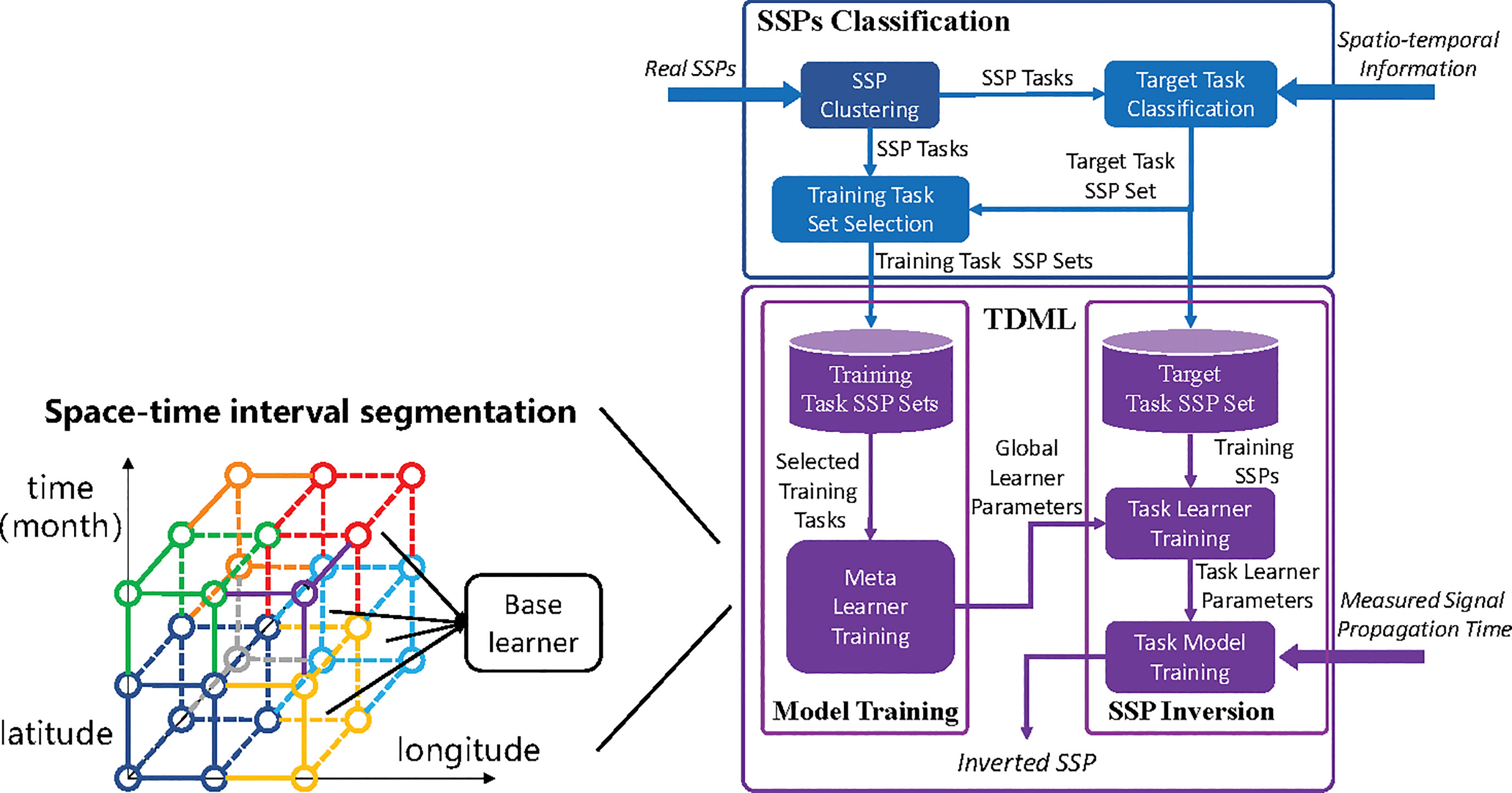
Figure 3 Task-driven Meta-learning Framework for SSP inversion.

Considering the spatio-temporal difference of SSP distribution, the ocean region is divided according to spatio-temporal information. A base learner is established for each region, and different types of SSPs obtained by clustering are also allocated to each spatio-temporal interval according to the spatio-temporal information of the cluster center, which could be used as training data. The spatio-temporal division scales are usually in varied forms, however, in this paper, the space is divided by 1 degree and time is divided by month.

In the proposed TDML framework, several kinds of learning models could be used as the base learner or task learner such as neural networks in Benson et al. (2000); (Huang et al., 2018; Huang et al., 2021) and Gaussian process in Yin et al. (2020). In order to guarantee a good robustness performance, the auto-encoding feature-mapping neural network (AEFMNN) proposed in our early work Huang et al. (2021) is utilized as the base and task learners. When the measured signal propagation time is fed into the trained task learner, the inversion SSP could be quickly obtained with once forward propagation.

4.1 SSPs clustering and task mapping

4.1.1 Pearson-correlation-based SSP local density clustering

The difference of SSP behaves in the variation trend of sound speed values with depth. To obtain SSP clusters with similar distribution, we propose a PC-SLDC algorithm, the structure of which is given in Figure 4. The SSPs distribution in the ocean is continuous, if the clusters of SSPs are divided without overlapping, the task SSP whose real distribution is at the margin of the cluster domain may not be accurately estimated because the reference data in this cluster is not uniformly or symmetrically distributed around the task SSP (as shown in Figure 4), which may lead to overfitting problem. Therefore, its better to cluster SSPs with partly overlapping. In this case, the SSP sample that lays at the margin of a cluster domain may belong to another cluster at the same time.

FIGURE 4

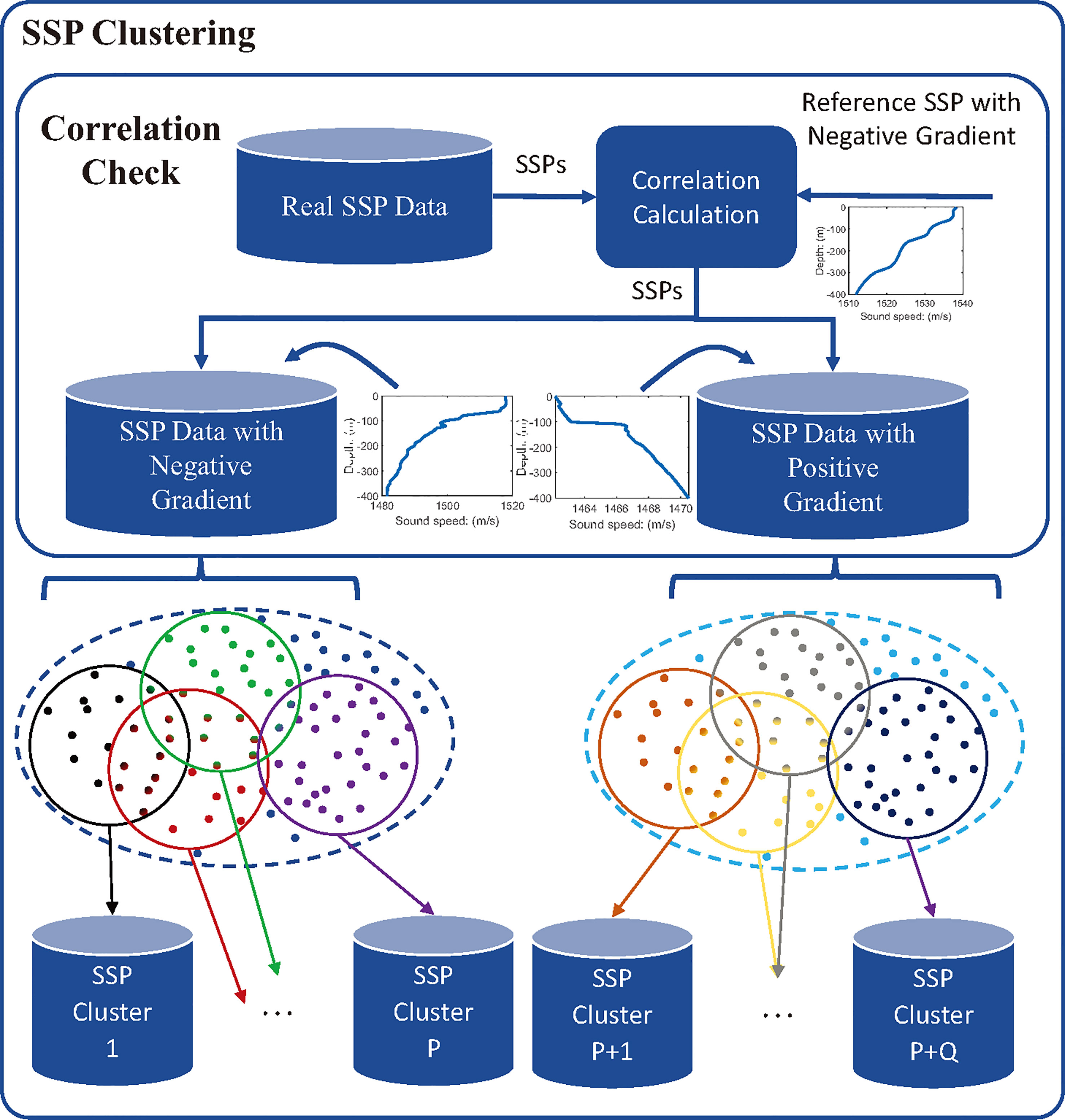
Figure 4 SSP Local density clustering method based on Pearson correlation test.

Euclidean distance has been widely adopted to describe the difference between two SSPs such as Choo and Seong (2018); Zhang et al. (2015)¹, but it can not reflect whether the variation trends with depth of two SSPs are consistent or not, especially for shallow-water SSPs that their gradients may be positive or negative. Therefore, a correlation check process is first established, in which a standard SSP with negative gradient is introduced as a reference to calculate the Pearson correlation coefficient between each historical SSP data and the reference one. Assume the reference SSP is $S_r={[(s_r^1,1),(s_r^2,2),\dots ,(s_r^d,d)]}^T$, and the $i$th original SSP is $S_{o_i}={[(s_{o_i}^1,1),(s_{o_i}^2,2),\dots ,(s_{o_i}^d,d)]}^T$, where $d$ is the depth of corresponding sound speed in meters², the Pearson correlation coefficient ${\rho }_{r,o_i}$ can be calculated by:

$\begin{array}{ll}{\rho }_{r,o_i}=\frac{{\displaystyle \sum _{d=1}^D\left(s_r^d-u_r\right)\left(s_{o_i}^d-u_{o_i}\right)}}{\sqrt{{\displaystyle \sum _{d=1}^D{\left(s_r^d-u_r\right)}^2}}\sqrt{{\displaystyle \sum _{d=1}^D{\left(s_{o_i}^d-u_{o_i}\right)}^2}}},& (4)\end{array}$

where $u_r=\frac{1}{D}{\displaystyle \sum _{d=1}^D{s}_r^d}$ is the average sound speed of SSP $S_r$, and $u_{o_i}=\frac{1}{D}{\displaystyle \sum _{d=1}^D{s}_{o_i}^d}$ represents the average sound speed of SSP $S_{o_i}$. With equation (4), all historical SSP data ${\mathcal{S}}_O=\left\{S_{o_1},S_{o_2},\dots ,S_{o_i}\right\},i=1,2,\dots ,I$ will be divided into two group: the SSP group ${\mathcal{S}}_{O^{-}}$ with negative gradient or the SSP group ${\mathcal{S}}_{O^{+}}$ with positive gradient.

After the correlation check, the SSPs in each subset could be further clustered into different groups based on the Euclidean distance. If $S_{o_1^{-}}={[(s_{o_1^{-}}^1,1),\dots ,(s_{o_1^{-}}^d,d)]}^T$and $S_{o_2^{-}}={[(s_{o_2^{-}}^1,1),\dots ,(s_{o_2^{-}}^d,d)]}^T$are both SSPs in ${\mathcal{S}}_{O^{-}}$, the Euclidean distance $e_{o_1^{-},o_2^{-}}$ is calculated as:

$\begin{array}{ll}{e}_{o_1^{-},o_2^{-}}=\sqrt{\sum _{d=1}^D{\left(s_{o_1^{-}}^d-s_{o_2^{-}}^d\right)}^2}.& (5)\end{array}$

Similarly, for $S_{o_1^{+}}={[(s_{o_1^{+}}^1,1),\dots ,(s_{o_1^{+}}^d,d)]}^T$ and $S_{o_2^{+}}={[(s_{o_2^{+}}^1,1),\dots ,(s_{o_2^{+}}^d,d)]}^T$ in ${\mathcal{S}}_{O^{+}}$, the Euclidean distance $e_{o_1^{+},o_2^{+}}$ can be calculated as:

$\begin{array}{ll}{e}_{o_1^{+},o_2^{+}}=\sqrt{\sum _{d=1}^D{\left(s_{o_1^{+}}^d-s_{o_2^{+}}^d\right)}^2}.& (6)\end{array}$

For classical K-means clustering algorithm or density-based spatial clustering (DBSCAN) algorithm, one sample is usually classified into one class. However, repetitive clustering of SSP is allowed in PC-SLDC algorithm, the details of which is given in Algorithm 1.

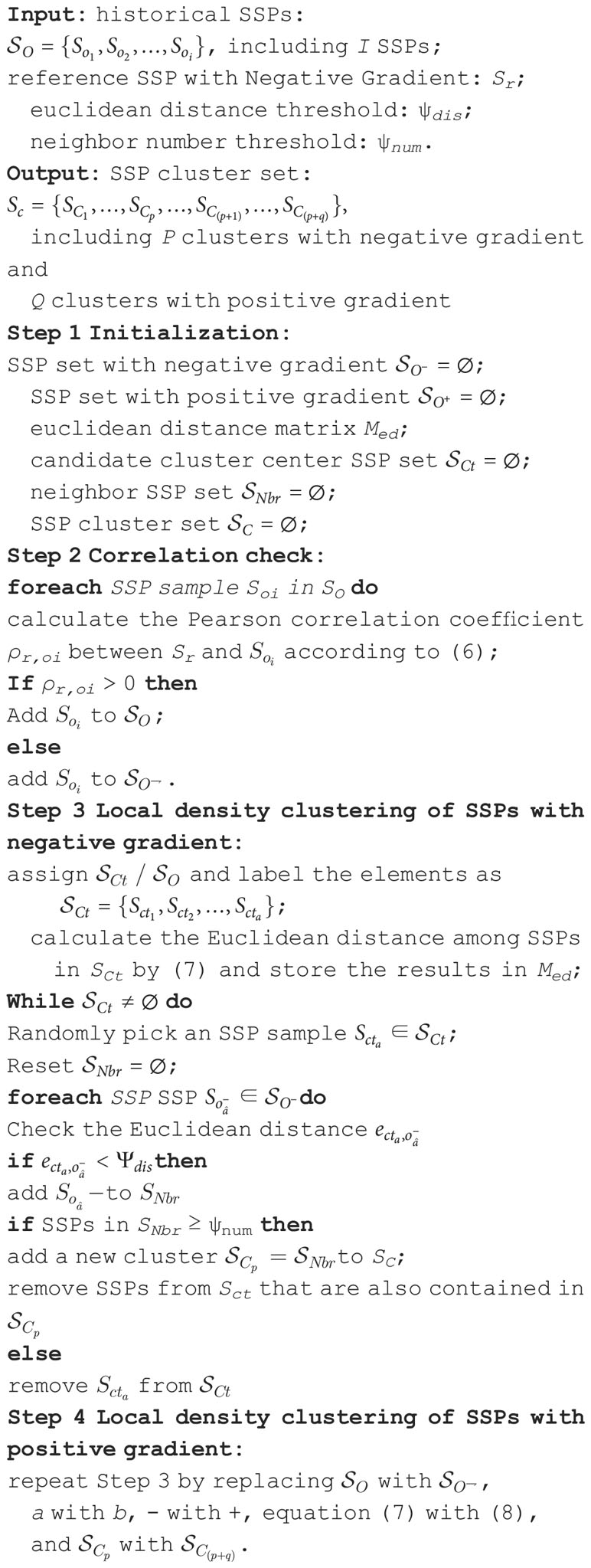
Algorithm 1. Pearson-correlation-based SSP local density clustering algorithm

At the beginning, all unclassified SSPs in${\mathcal{S}}_{O^{-}}$ have the opportunity to become a new class center and they form a candidate cluster center set ${\mathcal{S}}_{Ct}$. The Euclidean distance between each other is calculated through (5) and stored in an Euclidean distance matrix $M_{ed}$. An SSP sample $S_{c{t}_a}\in {\mathcal{S}}_{Ctr}$ is randomly picked up, if the Euclidean distance between any SSP $S_{o^{-}}\in {\mathcal{S}}_{O^{-}}$ and the current candidate center $S_{c{t}_a}$ is less than a threshold ${\text{Ψ}}_{dis}$, then the former will be a neighbor of the latter and added to a neighbor SSP set ${\mathcal{S}}_{Nbr}$. If the number of SSPs in ${\mathcal{S}}_{Nbr}$ exceeds a certain threshold ${\text{Ψ}}_{num}$, the current candidate point $S_{c{t}_a}$ will be taken as the true center to establish a group ${\mathcal{S}}_{C_p}$, and all neighbors are added into ${\mathcal{S}}_{C_p}$. Otherwise, $S_{c{t}_a}$ will be removed from ${\mathcal{S}}_{Ct}$ and a new candidate center SSP will be chosen to repeat theabove process. The whole process will be done again for SSPs in ${\mathcal{S}}_{O^{+}}$.

4.1.2 Spatio-temporal-information-based target task mapping

For a specified SSP inversion task, those historical sampled SSPs having the similar distribution with the target task is suitable for training the task inversion model. However, the sound speed distribution of the target task is not a prior information, thus the potential training SSPs can not be found according to the distribution features of SSPs. Since that the distributions of SSPs are similar when these SSPs are sampled with close spatio-temporal information, the search of suitable training data can be realized based on the similarity of spatio-temporal information.

For target task mapping, we propose an STI-KNN task mapping algorithm to find proper reference data for the task inversion model, and the prior SSP clusters ${\mathcal{S}}_C$ is obtained by Algorithm 1. When an inversion task is assigned, we define a spatio-temporal distance parameter $\varphi$ to describe the similarity between the sampling regions of a reference SSP and the task, which can be expressed as:

$\begin{array}{ll}\varphi =\lambda *{\varphi }_{\alpha }+(1-\lambda )*{\varphi }_{\beta },& (7)\end{array}$

where ${\varphi }_{\alpha }$ is the sampling time difference, ${\varphi }_{\beta }$ is the sampling location difference, and $0\le \lambda \le 1$ is a factor to balance ${\varphi }_{\alpha }$ and ${\varphi }_{\beta }$.

The ${\varphi }_{\alpha }$ is calculated by:

$\begin{array}{ll}{\varphi }_{\alpha }=\{\begin{array}{l}\left|{\alpha }_t-{\alpha }_o\right|,if\left|{\alpha }_t-{\alpha }_o\right|<183\hfill \\ 365+\min ({\alpha }_t,{\alpha }_o)-\max ({\alpha }_t,{\alpha }_o),otherwise\hfill \end{array}& (8)\end{array}$

where ${\alpha }_t$ and ${\alpha }_o$ are the time information of SSP inversion task and a random SSP in ${\mathcal{S}}_O$ (Algorithm 1), respectively. Due to the high similarity of SSPs sampled at the same period in different years within a certain area, it is not necessary to distinguish the year differences, thus the sampling time information is defined in days. If an SSP is collected on February 1, the sampling time value equals to 32, because the 1st day on February is the 32th day of the year. However, it should be noted that the time difference will not exceed half a year (183 days), because the time code is cyclic. For instance, assume two SSPs are sampled on October 1 in the last year (the 244th day of a year) and January 1 in the current year (the 1st day of a year), the actual time difference is $365+1-244=122$, but not $244-1=243$. This is because the 1st day of the last year is equal to the 1st day of the current year, which could be virtually regarded as the 366th day of the last year (without lose of generality, the leap year is taken as an example).

The space information is defined by the latitude and longitude coordinate of an SSP. The ${\varphi }_{\beta }$ is calculated by:

$\begin{array}{ll}{\varphi }_{\beta }=\sqrt{{({\beta }_t^x-{\beta }_o^x)}^2+{({\beta }_t^y-{\beta }_o^y)}^2},& (9)\end{array}$

where subscript $t$ and $o$ have the same meaning as (8), ${\beta }^x$ and ${\beta }^y$ represent the longitude and latitude coordinates of SSP sampling space after coding, respectively. As we focus on the distribution of sound speed in the Pacific Ocean of the Northern Hemisphere, the coded ${\beta }^y$ equals to the SSP’s latitude coordinate, while ${\beta }^x$ is defined as:

$\begin{array}{ll}{\beta }^x=\{\begin{array}{l}\left|{\widehat{\beta }}^x\right|-180,if{0}^{\circ }E<{\widehat{\beta }}^x<{180}^{\circ }E\hfill \\ 180-\left|{\widehat{\beta }}^x\right|,if{0}^{\circ }W<{\widehat{\beta }}^x<{180}^{\circ }W\hfill \end{array}& (10)\end{array}$

where ${\widehat{\beta }}^x$ is the original longitude coordinate of the SSP.

After comparing the spatio-temporal distance between all historical SSPs and the target SSP, the cluster which contains most of the $\kappa$ nearest SSPs will be determined as the mapping result of the target task. The factor λ in (7) is determined through random verifications, which is conducted based on real sampled SSP data from WOD’18 in the Pacific Ocean with different kinds of distribution. Through these random verifications, the accuracy of mapping the target task to the exact cluster, that has similar SSP distribution with the task, will be statistically tested under different $\lambda$ values, and the most appropriate $\lambda$ will be determined according to the highest mapping accuracy.

The training data for an SSP inversion task can be artificially provided or automatically selected by machine learning algorithms. For automated SSP inversion system with much less human cost, the lambda will affect the probability of providing suitable training data for the task learner. Since the SSPs with different distribution compared with those of the task area will mislead the learning process of task learner, the inversion accuracy will decrease when the SSP cluster of the task is wrongly mapped. Therefore, the task mapping accuracy that corresponding to the factor $\lambda$ indicates the confidence coefficient of an inverted SSP result. The STI-KNN algorithm is given in Algorithm 2.

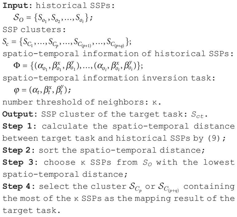
Algorithm 2. STI-KNN task mapping algorithm

4.2 Task-driven meta-learning

To solve the over-fitting problem and increase the SSP inversion accuracy with few-shot reference samples, we propose a TDML SSP inversion model as shown in Figure 5 that includes a meta-training phase and an SSP inversion phase. There is a global learner, several base learners and a task learner in the proposed model. Through $K$ base learners each trained with V-shot SSPs from different clusters, which is called K-way V-shot learning, a good set of initialization parameters for the global learner is found, so that the task learner initialized by the global learner could converge quickly with a few training times on the task SSP training set.

FIGURE 5

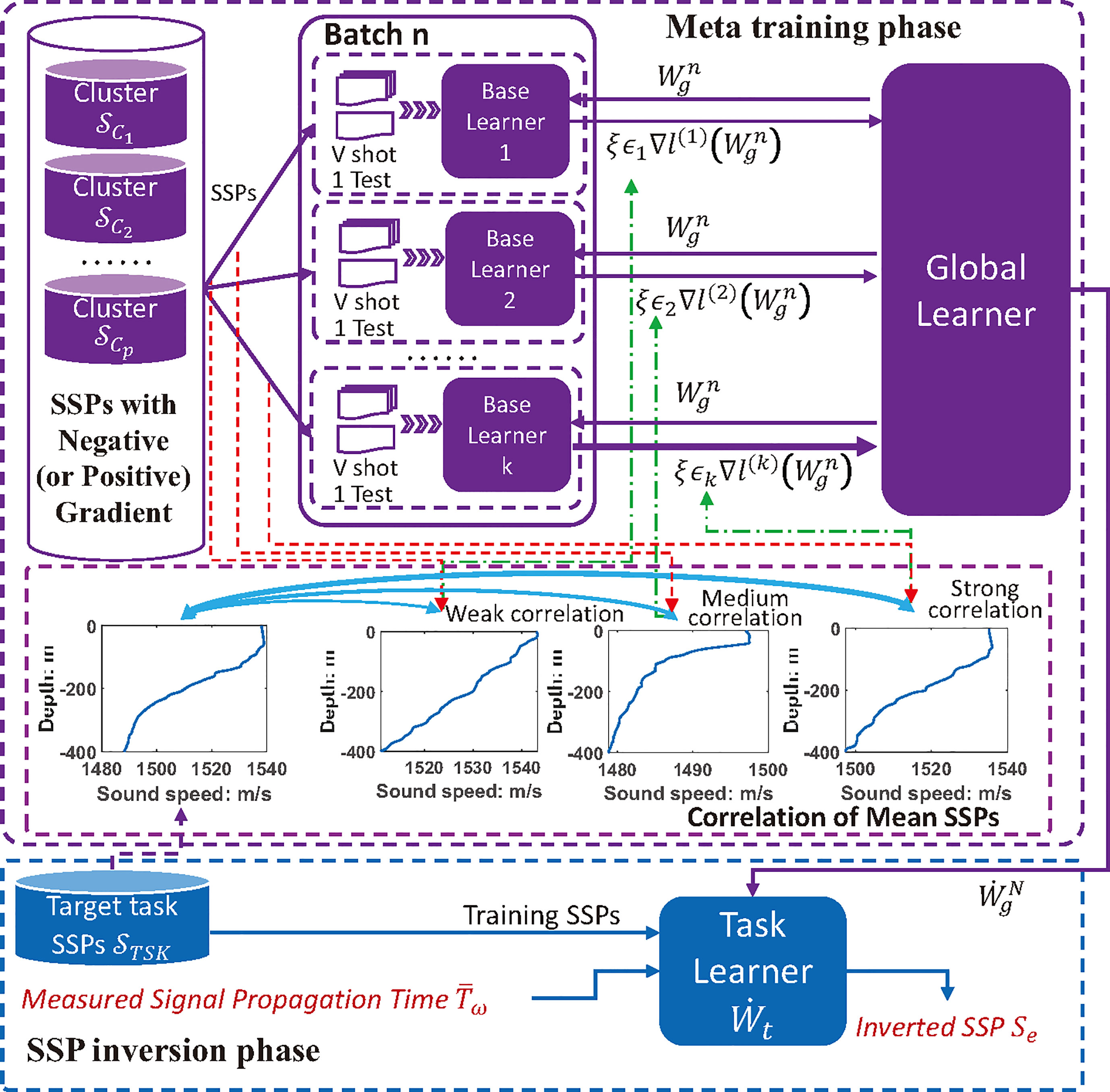
Figure 5 Task-driven meta-learning model for SSP inversion.

According to the SSP clustering result by the proposed PC-SLDC algorithm, the SSP distribution of the target task is either positive or negative, and the base learner trained by SSPs with the opposite gradient will contribute negatively to the global learner, which will slow down the convergence progress of the task model, even decrease the inversion accuracy. To diminish the negative transfer, the SSP clusters that having the same gradient direction with that of the task SSP set are chosen as the candidate training sets for base learners. Moreover, if the distribution of SSPs learned by the base learner $k$ is more similar to that of the task training SSPs, the base learner $k$ will have more influence on the parameter updating of the global learner, which is achieved by adjusting the gradient learning rate. Thus, the negative transfer could be further weakened, and the task learner could converge faster so as to avoid over-fitting on few-shot reference samples.

Concretely, we propose a TDML SSP inversion algorithm to illustrate the model training and application process. The neuron connection parameter of global learner is randomly initialized as $W_g^1$ while updated iteratively. At the beginning of the $n$th batch³, all the $K$ base learners are initialized by the global learner $W_g^n$, meanwhile, $K$ SSP clusters are randomly chosen from the $P$ available training SSP clusters ($K\le P$) for training the $K$ base learners respectively, each of which consists of $1$ testing and $V$ training samples. For base learner $k$, the $V$ SSPs are used forone step learning with the lose function defined as:

$\begin{array}{ll}{l}^{(k)}\left(W_k^n\right)=\sum _{v=1}^V\left(\frac{1}{2}\sum _{d=1}^D{\left(s_v^d-{\tilde{s}}_v^d\right)}^2+{\Vert W_k^n\Vert }_1\right),W_k^n=W_g^n,& (11)\end{array}$

where $s_v^d$ is the sound speed of the $v$th training SSP at depth $d$, ${\tilde{s}}_v^d$ is the corresponding inverted sound speed, and $W_k^n{}_1$ is the regularization item of the base learner $k$. Next, the local parameters are updated with back propagation (BP) algorithm by Rumelhart et al. (1986):

$\begin{array}{ll}{\dot{W}}_k^n=W_k^n-\eta {\nabla }_{W_k^n}{l}^{(k)}(W_k^n),& (12)\end{array}$

where $\eta$ is the learning rate of base learners. Then, the base learner is test on the left 1 SSP data $S_{tst}$ with lose function:

$\begin{array}{ll}{l}^{(k)}\left({\dot{W}}_k^n\right)=\frac{1}{2}\sum _{d=1}^D{\left(s_{tst}^d-{\tilde{s}}_{tst}^d\right)}^2,& (13)\end{array}$

where $s_{tst}^d$ and ${\tilde{s}}_{tst}^d$are the sound speed of the testing and inverted SSP, respectively. Finally, the parameters of the global learner are updated by optimizing the performance $L$ with respect to $W_g^n$($W_g^n=W_k^n$) across all base learners. The global optimization problem is expressed as follows:

$\begin{array}{ll}\underset{W_g^n}{\min }L=\underset{W_g^n}{\min }\sum _{k=1}^K{l}^{(k)}\left({\dot{W}}_k^n\right).& (14)\end{array}$

Note that the meta-optimization is performed over the initial parameter $W_g^n$ during current iteration, whereas the objective is computed using the updated parameters ${\dot{W}}_k^n$. In this way, the sensitivity of the model could be enhanced so that one or a small number of gradient updating steps on a new task will produce maximally effective behavior on that task according to Finn et al. (2017).

To further improve the quality of initialization parameters learned by the global learner, a correlation coefficient ${⋲}_k(k=1,2,\dots ,K)$ is introduced into each base learner to adjust the updating speed of model parameters, which is concretely the Pearson correlation coefficient between the mean SSP of the $k$th meta training cluster and the mean SSP of the inversion task training SSPs. With the K-way V-shot training, the meta-optimization is actually performed through stochastic gradient descent, such that the global learner is updated by:

$\begin{array}{ll}{\dot{W}}_g^n=W_g^n-\xi {\nabla }_{W_g^n}\sum _{k=1}^K{⋲}_k{l}^{(k)}\left({\dot{W}}_k^n\right),& (15)\end{array}$

where ${\dot{W}}_g^n$ represents the global leaner after parameter updating, and $\xi$ is the global learning rate. If the meta training is not over, the parameters of global learner in the $(n+1)$ th batch will be initialized as $W_g^{n+1}={\dot{W}}_g^n$.

After meta-training, the parameters of global learner ${\dot{W}}_g^N$ is transfer as the initialization for the task learner, so that $W_t^1={\dot{W}}_g^N$. Then the task learner is trained on a few training SSPs by one or a small number of steps, and the converged model is parameterized as ${\dot{W}}_t$. When feeding measured sound field information such as signal propagation time into model $W_t$, the inverted SSP ${\tilde{S}}_e$ can be estimated via once forward propagation, thereby improving the inversion efficiency. The detailed TDML algorithm for SSP inversion is given in Algorithm 3.

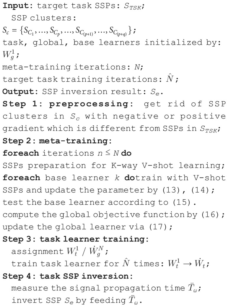
Algorithm 3. Task-driven meta-learning algorithm for SSP inversion

To reduce the impact of the time measurement error on the inversion model, which is caused by inaccurate positioning of the communication system, the joint AEFMNN and ray tracing model proposed in our previous work Huang et al. (2021) is introduced as the basic learning model for the base and task learner, and the anti-noise performance of TDML is inherited. In Huang et al. (2021), the robust feature extraction performance of the autoencoder has been evaluated by comparing the variation trend of correlation coefficients on the input signals and implicit features under different levels of time measurement error, in which the positioning error of AUVs is set to be zero for simulating a single error source. The signal propagation time correlation coefficients are calculated by correlating the error-influenced signal propagation time with the ideal one, and the correlation coefficient of implicit features is obtained via correlations between the implicit features extracted when the input signal propagation time is influenced by the measurement errors or without errors. Detailed anti-noise performance of AEFMNN can be referred to Figure 12 in Huang et al. (2021).

The learning model of base and task learner is given in Figure 6. There are total 7 layers in AEFMNN model that have been described in detail by Huang et al. (2021): noisy time input layer $T_{v,\omega }$, encoding hidden layer $F_{ec}$, decoding hidden layer $F_{dc}$, decoding time output layer ${\tilde{T}}_v$, translating hidden layer $F_{tr}$, translating output SSP layer ${\tilde{S}}_v$, and the hidden feature layer $F_{ed}$ shared by the encoder, decoder and translation neural network.

FIGURE 6

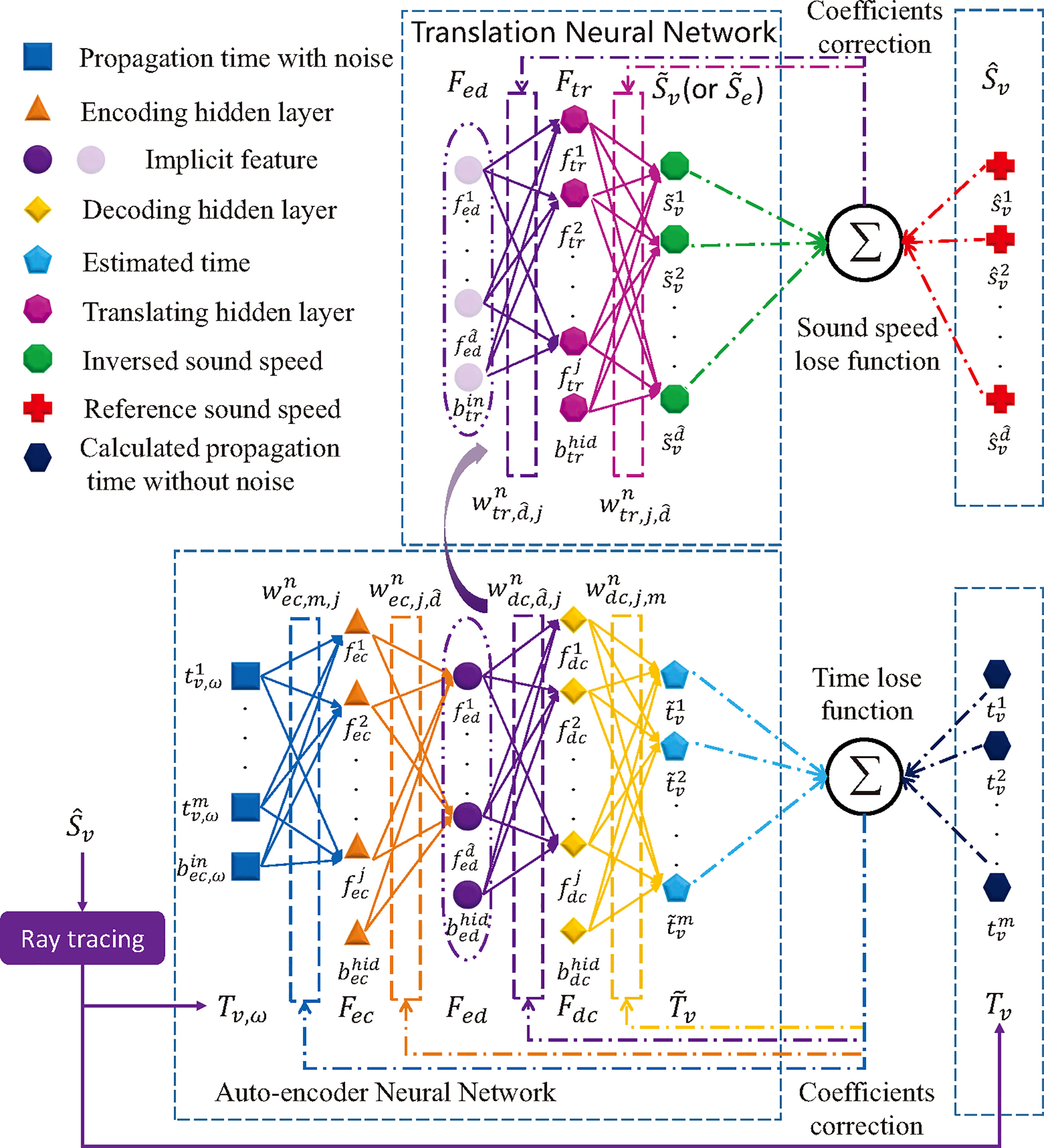
Figure 6 Joint Ray Tracing and AEFMNN SSP inversion model by Huang et al., 2021.

In Figure 6, the signal propagation time with measurement errors $T_{v,\omega }$ is simulated to reflect the real situation, while the one without errors ${\tilde{T}}_v$ is computed to be the labeled time information for updating the parameters of the auto-encoder. The auto-encoder and the translation neural network are updated in turn during once training. Through narrowing the gap between the estimated signal propagation time ${\tilde{T}}_v$ and the simulated time $T_v$, the auto-encoder is first trained to extract the implicit features that reduces the impact of measurement errors of the input data. Then by narrowing the gap between the inverted SSP ${\tilde{S}}_v$ and the labeled SSP ${\widehat{S}}_v$, the translation neural network is trained to establish the mapping relationship from the implicit features to the sound speed distribution.

Taking the $n$th iteration (V-shot) for base learner $k$ as an example, the parameters of the auto-encoder is updated by BP algorithm with the time lose function $l_t^{(k)}(W_k^n)$ expressed as:

$\begin{array}{ll}{l}_t^{(k)}\left(W_k^n\right)=\sum _{v=1}^V\left(\frac{1}{2}\sum _{m=1}^M{\left({\tilde{t}}_v^m-t_v^m\right)}^2+{\Vert W_{k,ec,dc}^n\Vert }_1\right),& (16)\end{array}$

where ${\tilde{t}}_v^m$ is the estimated signal propagation time of the $m$th receiver, $t_v^m$ is the corresponding theoretical time information without noise, and $W_{k,ec,dc}^n$ is the regularization item related to the parameters of the auto-encoder. Then, the translation neural network transform the hidden features to sound speed distribution with lose function (11) modified as:

$\begin{array}{ll}{l}^{(k)}\left(W_k^n\right)=\sum _{v=1}^V\left(\frac{1}{2}\sum _{d=1}^D{\left({\tilde{s}}_v^{\widehat{d}}-{\widehat{s}}_v^{\widehat{d}}\right)}^2+{\Vert W_{k,tr}^n\Vert }_1\right),& (17)\end{array}$

where ${\tilde{s}}_v^{\widehat{d}}$ is the inverted sound speed at depth $\widehat{d}$, ${\widehat{s}}_v^{\widehat{d}}$ is the corresponding labeled sound speed, and $W_{k,tr}^n$ is the regularization item related to the parameters of the translation neural network. The forward propagation process of AEFMNN is done by following equations:

$\begin{array}{ll}{f}_{ec}^j=\text{Γ}\left(\sum _{m=1}^M\left(t_{v,\omega }^m·w_{ec,m,j}^n\right)+b_{ec,\omega }^{in}·w_{ec,b,j}^n\right),& (18)\end{array}$

$\begin{array}{ll}{f}_{ed}^{\widehat{d}}=\text{Γ}\left(\sum _{j=1}^J\left(f_{ec}^j·w_{ec,j,\widehat{d}}^n\right)+b_{ec}^{hid}·w_{ec,b,\widehat{d}}^n\right),& (19)\end{array}$

$\begin{array}{ll}{f}_{dc}^j=\text{Γ}\left(\sum _{\widehat{d}=1}^{\widehat{D}}\left(f_{ed}^{\widehat{d}}·w_{dc,\widehat{d},j}^n\right)+b_{dc}^{in}·w_{dc,b,j}^n\right),b_{dc}^{in}=b_{ed}^{hid},& (20)\end{array}$

$\begin{array}{ll}{\tilde{t}}_v^m=\text{Γ}\left(\sum _{j=1}^J\left(f_{dc}^j·w_{dc,j,m}^n\right)+b_{dc}^{hid}·w_{dc,b,m}^n\right),& (21)\end{array}$

$\begin{array}{ll}{f}_{tr}^j=\text{Γ}\left(\sum _{\widehat{d}=1}^{\widehat{D}}\left(f_{ed}^{\widehat{d}}·w_{tr,\widehat{d},j}^n\right)+b_{tr}^{in}·w_{tr,b,j}^n\right),b_{tr}^{in}=b_{ed}^{hid},& (22)\end{array}$

$\begin{array}{ll}{\tilde{s}}_v^{\widehat{d}}=\text{Γ}\left(\sum _{j=1}^J\left(f_{tr}^j·w_{tr,j,\widehat{d}}^n\right)+b_t^{hid}·w_{tr,b,\widehat{d}}^n\right).& (23)\end{array}$

where the special subscript $b$ of the weight parameter $w$ indicates that the weight connects the bias neuron of current layer and the neurons in next layer. Among (18) to (23), the leaky rectified linear unit (LReLU) by Maas et al. (2013) is introduced as the activation function, which is expressed as:

$\begin{array}{ll}\text{Γ}(\tau )=\{\begin{array}{rr}\hfill \tau & \hfill \tau >0\\ \hfill \zeta \tau & \hfill \tau \le 0\end{array}& (24)\end{array}$

where $\zeta$ is a fixed constant between $-1$ and $0$ (0.25 in this paper).

The outputs of the translation neural network are the sound speeds at different depth, so the number of output neurons depends on the sampling depth of the SSP. If there are too many sampling points in an SSP, the required parameters of the neural network will increase significantly, thereby leading to the over-fitting problem when trained on few-shot dataset. To reduce the model complexity, an stratified-line SSP simplification algorithm proposed in our previous work Huang et al. (2019) is introduced, by which an original SSP $S_v$ could be accurately approximated to be ${\widehat{S}}_v$ via a few feature points.

5 Simulation and discussion

In this section, the performance of the proposed PC-SLDC algorithm for SSP clustering, the accuracy of task mapping with STI-KNN algorithm, the SSP inversion efficiency and accuracy under TDML framework are verified by simulations on historical SSP data in the shallow Pacific ocean with water depth of 400 m. However, the application is not limited to the experimental area, but also applicable to shallow or deep ocean where the sound speed distribution is consistent in a certain spatio-temporal range and the sound speed at each depth layer approximately obeys Gaussian distribution with the root-mean-square error (RMSE) on the order of a few meters per second. The experiments are done via Matlab “R2019a”, and all SSPs are real sampled in the Pacific Ocean that come from the WOD’18 Boyer et al. (2021), the sonar data used for SSP inversion is simulated through ray theory.

5.1 Accuracy of target task mapping

To guarantee the convergence performance of the learning model, the i.i.d. condition of training and testing data needs to be satisfied. Therefore, similarly clustering the empirical SSPs and finding which cluster the target task belongs to become extremely important. To evaluate the performance of proposed PC-SLDC and STI-KNN algorithms, we first divide the SSPs into clusters base on PC-SLDC, then test the target task mapping accuracy by STI-KNN, finally compare the SSP similarity under different clustering criteria.

In Figure 7, the mapping accuracy of STI-KNN algorithm for target task is tested on 391 historical SSPs sampled in the Northern Pacific Ocean with each checking 7 neighbor SSP samples. When the Euclidean density distance threshold is set to be ${\text{Ψ}}_{dis}\le 10$ and the element number of clusters is set to be ${\text{Ψ}}_{num}\ge 15$ in PC-SLDC, the accuracy of STI-KNN can be up to 96% with $\lambda =0.02$. When the Euclidean density distance threshold is set to be ${\text{Ψ}}_{dis}\le 8$ andthe element number of clusters is set to be ${\text{Ψ}}_{num}\ge 12$ in PC-SLDC, the accuracy of STI-KNN can be up to 97.85% with $0.01\le \lambda \le 0.036$. The $\lambda$ is set to be $0.02$ in our following simulations, and SSPs are clustered with $s{i}_{dis}\le 10,{\text{Ψ}}_{num}\ge 15$.

FIGURE 7

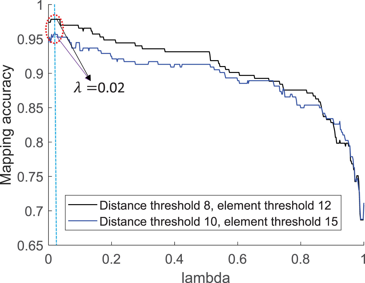
Figure 7 Mapping accuracy of SSP inversion task by STI-KNN algorithm.

After target task mapping, we evaluate the clustering performance by testing the error distances of $20$ samples to the mean SSP of the cluster that each sample maps to via STI-KNN as shown in Figure 8, the cluster of which is obtained by PC-SLDC and compared with clustering merely by SSP sampling month or location. The SSPs of items 1, 2 and 3 are the same group with negative gradients, while the SSPs of items 4, 5 and 6 are the same group with positive gradients. The location threshold is $5$ longitude and latitude, and the month threshold is $1$ month. From the result, the SSPs clustered through PC-SLDC are more similar to their cluster elements than SSPs clustered merely by month or location information. In particular, the RMSE of test SSPs to the mean SSP of the cluster obtained by month is much worse than the other two, this is because the empirical SSPs within each month are sampled dispersedly around the Northern Pacific Ocean, the distributions of which are obviously different.

FIGURE 8

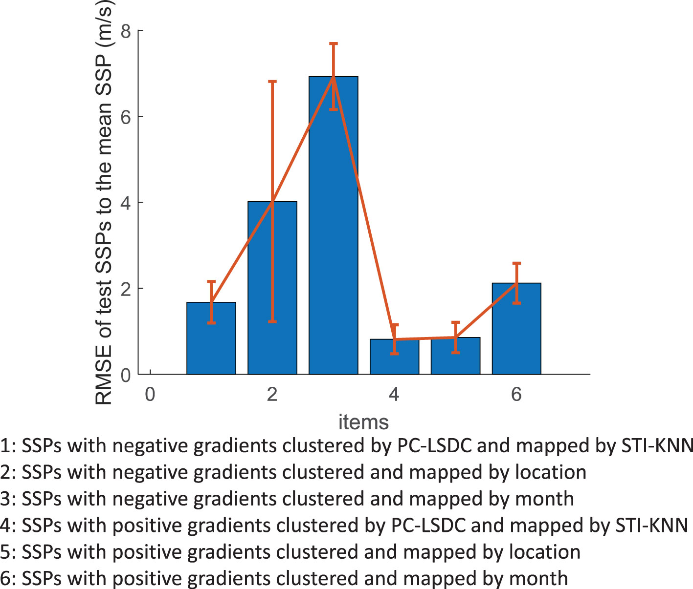
Figure 8 Error distances of SSPs to the average SSP of the task cluster.

The average SSP of each cluster can be used for roughly estimating the sound speed distribution of a certain area, however, the variation of sound speed can not be reflected in different regions or sampling date, and the estimation error of sound speed will increase with the area scale or time interval expanding. Therefore, it is necessary to further improve the accuracy of sound speed inversion by learning to establish the mapping relationship from signal propagation time to sound speed distribution.

5.2 SSP inversion under TDML framework

The TDML framework proposed in this paper aim to improve the SSP inversion accuracy while reduce the time as much as possible. In this section, we test the accuracy and time efficiency of the proposed TDML-based SSP inversion method compared with some classical SSP inversion methods as base lines.

5.2.1 Base lines and parameter settings

5.2.1.1 MFP-EOF-PSO

There are four steps included in this classical SSP inversion method: principal component extraction, candidate SSPs generation, simulated sound field calculation and sound field matching; the candidate SSP corresponding to the optimal matching sound field will be recorded as the final inversion result. Heuristic algorithms are widely used in searching for the matched item, and PSO is adopted as an example in this paper.

5.2.1.2 CS

The CS-based SSP inversion is a new method that is combined with EOF. In this method, the eigenvectors of EOF are utilized to form the compressed sensing dictionary.

5.2.1.3 AEFMNN-based single learning model

The single AEFMNN SSP inversion model has the same model structure with any base learner of TDML. Such a model is set up for comparing to evaluate the anti-over-fitting performance of TDML.

5.2.1.4 TL

TL is a classical method that can be used for few-shot learning. Two AEFMNN models having the same structure with base learners of TDML are introduced. One model is trained on SSPs that are not belong to the task cluster, while the other is trained by the task cluster; the trained parameters of the former model are set to be the initialization for the later model.

5.2.1.5 ML

The difference between ML and TDML for SSP inversion is that all SSP clusters, excluding the task cluster, can be used for meta-training in ML, while only SSP clusters having the same positive or negative gradients with the task cluster can be used for meta-training in TDML. By this means, we verify the performance of TDML against the negative migration.

The parameter settings of TDML are shown in Table 1. As the position error of the bottom AUV in Figure 9 is harmful for sound field measurement, the location should be modified before the measuring process. According to our previous work on ray-tracing-based positioning correction Huang et al. (2019), the bottom AUV can be relocated with the help of those surface AUVs according to the average sound speed distribution of the task area. Under 10000 times simulation tests, the location error can be reduced through ray tracing technique based on average empirical SSP distritbution Huang et al. (2019), and follows the Gaussian distribution with average error $0m$ and standard deviation less than $0.1m$ under the time measurement error level ${\sigma }_c=3ms$ (three surface AUVs form a equilateral triangle with 100 m between each other, and the position errors of surface AUVs are not considered). In reality, the location error of bottom AUV may be larger than simulated due to the topology chaning of surface AUVs and the movement of underwater flow. Since the AEFMNN is the basic inversion model introduced in this paper, the SSP inversion accuracy of all these methods will be influenced when the location error increases, however, the anti-overfitting performance and the convergence performance will still be different with these methods. Some specific parameter settings of base lines are given in Table 2.

TABLE 1

Table 1 Parameter settings of TDML.

FIGURE 9

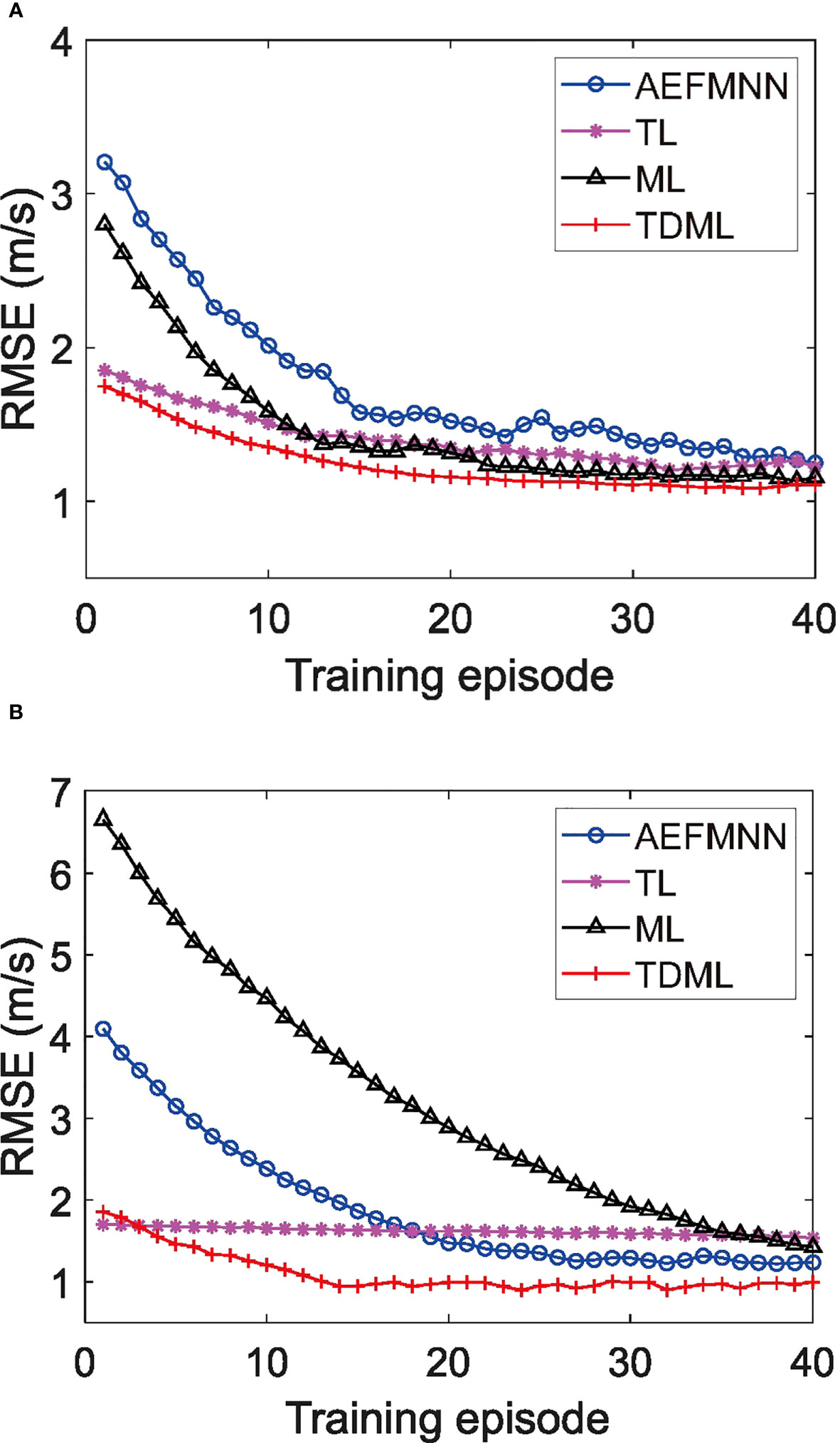
Figure 9 Convergence comparison of different deep learning methods for SSP inversion. (A) Cluster 1with negative gradients. (B) Cluster 2 with positive gradients.

TABLE 2

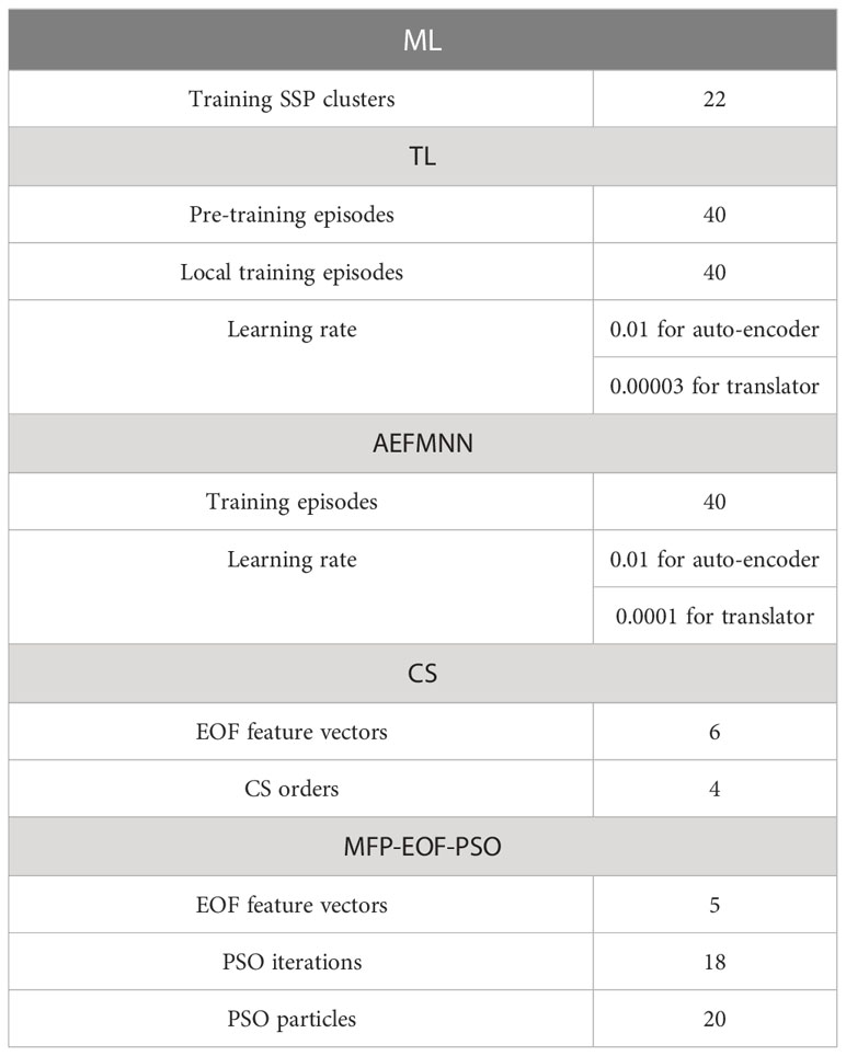
Table 2 Parameter settings of base lines.

5.2.2 Accuracy comparison

To verify the effectiveness of task mapping based on spatio-temporal information, the inversion average accuracy of TDML with $100$ testing times is compared with clustering criterion by location or month in Table 3. Results show that the TDML trained with clustering by month or location is hard to converge because the training samples in every cluster may be far different from each other, thus the inversion errors are much higher than the clustering by spatio-temporal information.

TABLE 3

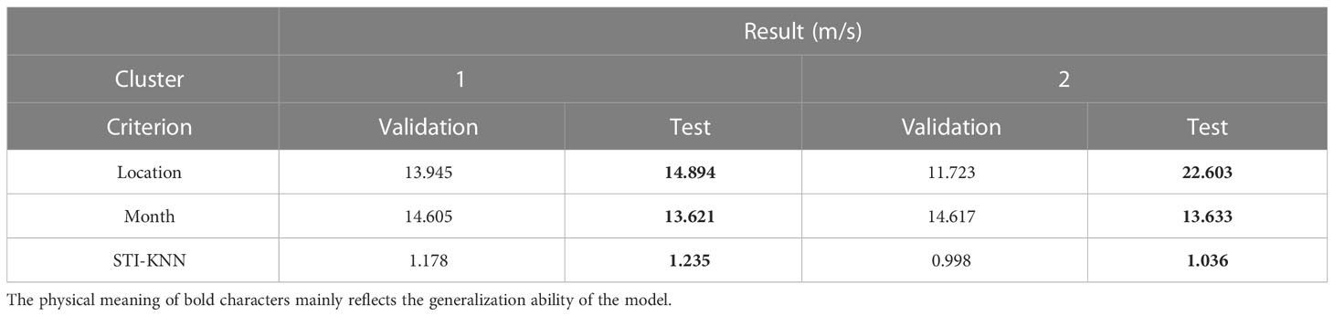
Table 3 RMSE OF SSP inversion by TDML based on different clustering criterion.

To evaluate the accuracy performance of TDML, the RMSE results of SSP inversion on two different clusters with negative or positive gradients are tested as examples in Table 4 compared with other inversion methods. The inversion results in Table 4 are average results with $100$ testing times. The results indicate that through leveraging sound field information such as signal propagation time, the SSP inversion accuracy behaves better than rough estimating by the average SSP of the cluster. Actually, the signal propagation time is a sensitive function of sound speed changes, while with measured signal propagation time, these changes can be seized to some extent by those SSP inversion methods.

TABLE 4

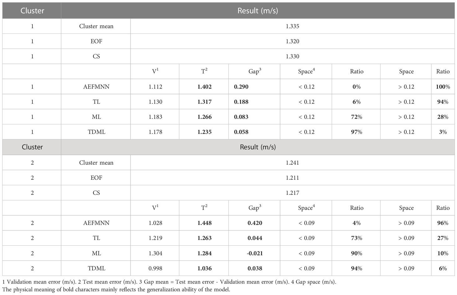
Table 4 RMSE of SSP inversion by different methods.

For evaluating the anti-over-fitting ability, both the SSP inversion accuracy during task training and testing processes are tested for deep-learning-based methods. Among these methods, the TDML performs best for testing SSP samples. The accuracy of SSP inverted by CS is a little worse than MFP (combined with EOF and PSO) due to the first-order Taylor linear approximation at the dictionary establishing process. Because of the scarcity of training samples after clustering by PC-SLDC, the SSP inversion via AEFMNN is prone to be over-fitting, which is why the training accuracy can be extremely high but the testing accuracy will be greatly reduced, and reflected in large test-validation values. For TL, ML and TDML, the anti-over-fitting capability is improved. However, it should be noted that the inversion accuracy by TL is not as good as ML or TDML, and this is mainly because the initialization parameters of the task model are pre-trained in different ways. For TL, the model is pre-trained by another SSP cluster, which makes it retain much characteristics of pre-training cluster when transferring model parameters, thereby reducing the ability to learn new SSP distribution. On the contrary, the ML or TDML is pre-trained by meta models to learn more public features among SSP clusters, and the second-order gradient descent by (15) makes the model more sensitive to the changes of signal propagation time. Therefore, the ML-based model is not likely to be over-fitting on pre-training SSP clusters.

For cluster 1, the accuracy improvement of TDML is not obvious compared with that of ML. In fact, this phenomenon is related to the training SSP clusters. Among the 22 training SSP clusters for ML, 18 clusters are distributed in negative gradient, which is the same with the target task cluster. To verify the resistance ability of TDML to negative migration, SSPs with positive gradient are chosen to be the target task, and the comparison of inversion accuracy with different methods is given in cluster 2. For ML, most of pre-training SSP clusters are distributed in negative gradient, so it is difficult for the ML model to learn the common features of SSPs with positive gradient, resulting in bad learning ability on the new task. On the contrary, the pre-training clusters for TDML are all distributed in positive gradient, the accuracy performance can be guaranteed.

To give a more intuitive understanding of the negative migration in ML, the convergence of inversion tasks belonging to cluster 1 and 2 are displayed in Figures 9A, B, respectively. It can be noticed that with TDML, the model can converge after only 20 times of training, which is much faster than other methods. In few-shot learning, reducing the repeated training of samples is helpful to deal with the over-fitting problem. For task cluster 1, the initial parameters of TDML for task learner are closer to the optimal solution than ML; while for task cluster 2, the negative migration of ML is so obvious that the initial parameter is far from the optimal solution, and the convergence rate is also significantly reduced. However, for TDML in Figures 9A, B, there are decreasing processes and exist turning points that the RMSE error (m/s) becomes stable after a few of training episodes. Especially, the gap between the beginning and the convergence stage of TDML is smaller in Figure 9B, which indicates that the TDML does work and forms a good set of initial parameters of the task model.

For intuitively expressing the inversion results, the SSP inversion example through different methods is given in Figure 10. The result of TDML has better fitting with the original SSP curve.

FIGURE 10

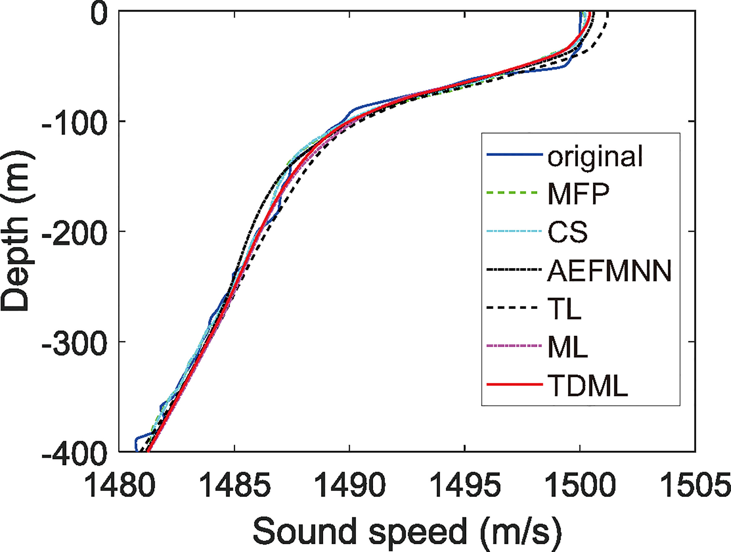
Figure 10 Time overhead of SSP inversion.

5.2.3 Time efficiency comparison

The time efficiency of inversion method is very important for emergency tasks such as underwater rescue. As the training of learning models could be finished offline before task assignment, more attention should be paid to the time overhead on the inversion stage, which is compared in Figure 11. The match sound field information needs to be searched by heuristic algorithms in MFP, which is very time-consuming. For CS-based method, several iterations are needed to gradually reduce the residual. However, for learning-based methods, only once forward propagation is enough to obtain the inverted SSP with a well trained model, so the time efficiency is enormously improved.

FIGURE 11

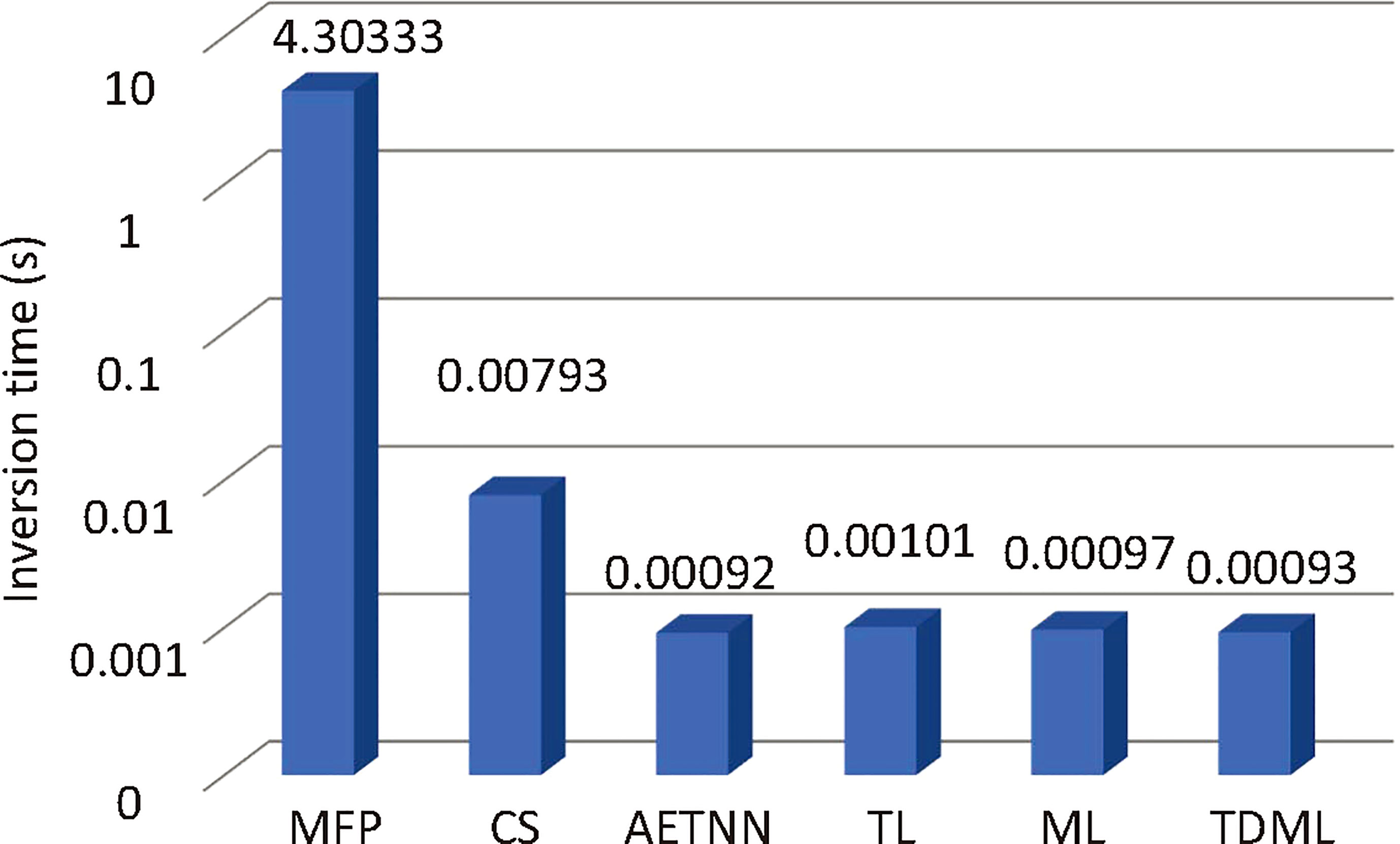
Figure 11 An example of SSP inversion result.

6 Conclusion

To satisfy the accurate and time-efficient requirements of underwater localization applications such as emergency rescue, we propose a TDML framework for fast and accurately estimating the regional SSP that is beneficial for positioning correction. The TDML can be competent for most ocean SSP inversion tasks, especially in few-shot learning scenarios. By simultaneously learning different kinds of SSPs with several base learners, the common features of SSPs can be captured and transferred to the task learner, and the sensitivity of the task learner to the unique characteristics of task SSPs can also be maintained. Thus, the model can converge quickly in the face of new SSP inversion tasks, so as to reduce the over-fitting effect in few-shot learning.

To guarantee the i.i.d conditions, we propose a PC-SLDC algorithm for clustering the empirical SSPs with similar distribution. Then we propose an STI-KNN algorithm to map the target inversion task, so that proper training samples for the task can be found. To address the negative learning problem in ML, only clusters having the positive correlation with the task can be chosen as training tasks, and the learning rates of different base learners change with the similarity between the meta training data and the task training data. The experiment results show that the TDML has better generalization ability compared with other learning methods for SSP inversion, that is, the good accuracy performance is not only obtained in the model training stage, but also maintained in the SSP inversion (testing) stage. Moreover, the TDML inherits the advantage of time efficiency of ANN during the inversion stage.

Although TDML has better accuracy performance compared with AEFMNN, TL, ML, there are still some factors that limit the performance of TDML. 1)High noise level of signal propagation time that beyond the bearing capacity of AEFMNN will affect the SSP inversion accuracy. 2)The mapping accuracy of a given task to the SSP distribution cluster it belongs to has great influence on the confidence coefficient performance of SSP inversion result. 3)The SSP inversion accuracy will be limited when the real SSP distribution of a given task lays out of distribution coverage of reference SSPs, though it is accurately mapped to a cluster. For example, assume the time of SSP inversion task and most of its neighbor reference SSPs with least spatio-temporal distance is ideally the same, however, the location of SSP inversion task is at the external margin of the area constructed by the sampling location of reference SSPs. In this case, the TDML will not able to accurately invert the SSP of the task due to the spatial difference of SSP distribution, the problem of which is also exist in other SSP inversion methods.

In our future work, we are going to further verify the TDML in both shallow and deep ocean experiments, and apply the TDML SSP inversion method to underwater positioning and navigation systems.

Data availability statement

The original contributions presented in the study are included in the article/supplementary material. Further inquiries can be directed to the corresponding author.

Author contributions

WH: conceptualization, methodology, formal analysis, investigation, software, original draft writing. FY: conceptualization, methodology. DL: writing review and editing. HZ: supervision, writing review and editing. TX: writing review and editing, project administration. All authors contributed to the article and approved the submitted version

Funding

This work was financially supported by Laoshan Laboratory (LSKJ202205104), China Postdoctoral Science Foundation (2022M722990), Qingdao Postdoctoral Science Foundation (QDBSH20220202061), National Natural Science Foundation of China (NSFC:62271459), National Defense Science and Technology Innovation Special Zone Project: Marine Science and Technology Collaborative Innovation Center (22-05-CXZX-04-01-02), and the Fundamental Research Funds for the Central Universities, Ocean University of China (202313036).

Conflict of interest

The authors declare that the research was conducted in the absence of any commercial or financial relationships that could be construed as a potential conflict of interest.

Publisher’s note

All claims expressed in this article are solely those of the authors and do not necessarily represent those of their affiliated organizations, or those of the publisher, the editors and the reviewers. Any product that may be evaluated in this article, or claim that may be made by its manufacturer, is not guaranteed or endorsed by the publisher.

Footnotes

1. ^ For SSP with fixed number of sampling points, Euclidean distance is equivalent to mean square error Choo and Seong (2018) and root mean square error Zhang et al. (2015) in describing vector difference, and they are positively correlated.
2. ^ The sampling depth interval of original SSP data from world ocean database 2018 (WOD’18) is meter
3. ^ During each iteration, the base learner is trained and updated by one batch, so the total number of batches is equal to the number of iterations

References

Alet F., Schneider M. F., Lozano-Perez T., Kaelbling L. P. (2020). “Meta-learning curiosity algorithms,” in International Conference on Learning Representation 2020 (ICLR), Addis Ababa, Ethiopia: OpenReview.net. 1–22. doi: 10.48550/arXiv.2003.05325

CrossRef Full Text | Google Scholar

Benson J., Chapman N. R., Antoniou A. (2000). Geoacoustic model inversion using artificial neural networks. Oceans 1, 446–451. doi: 10.1088/0266-5611/16/6/302

CrossRef Full Text | Google Scholar

Bianco M., Gerstoft P. (2017). Dictionary learning of sound speed profiles. J. Acoustical Soc. America 140, 1749–1758. doi: 10.1121/1.4977926

CrossRef Full Text | Google Scholar

Bianco M. J., Gerstoft P., Traer J., Ozanich E., Roch M. A., Gannot S., et al. (2019). Machine learning in acoustics: theory and applications. J. Acoustical Soc. America 146, 3590–3628. doi: 10.1121/1.5133944

CrossRef Full Text | Google Scholar

Boyer T., Baranova O., Coleman C., Garcia H., Grodsky A., Locarnini A., et al. (2021) World ocean database 2018. Available at: https://www.ncei.noaa.gov/access/648world-ocean-database/datawodgeo.html.

Google Scholar

Carroll P., Mahmood K., Zhou S., Zhou H., Xu X., Cui J.-H. (2014). On-demand asynchronous localization for underwater sensor networks. IEEE Trans. Signal Process. 62, 3337–3348. doi: 10.1109/TSP.2014.2326996

CrossRef Full Text | Google Scholar

Chang H., Han J., Zhong C., Snijders A. M., Mao J. (2018). Unsupervised transfer learning via multi-scale convolutional sparse coding for biomedical applications. IEEE Trans. Pattern Anal. Mach. Intell. 40, 1182–1194. doi: 10.1109/TPAMI.2017.2656884

PubMed Abstract | CrossRef Full Text | Google Scholar

Choo Y., Seong W. (2018). Compressive sound speed profile inversion using beamforming results. Remote Sens. 10, 1–18. doi: 10.3390/rs10050704

CrossRef Full Text | Google Scholar

Cobbe K., Klimov O., Hesse C., Kim T., Schulman J. (2019). “Quantifying generalization in reinforcement learning,” in Proceedings of the 36th International Conference on Machine Learning. (Long Beach, California, USA: PMLR) 97, 1282–1289 doi: 10.48550/arXiv.1812.02341

CrossRef Full Text | Google Scholar

Dinn D. F., Loncarevic B. D., Costello G. (1995). “The effect of sound velocity errors on multi-beam sonar depth accuracy,” in ‘Challenges of Our Changing Global Environment’. Conference Proceedings, OCEANS’95 MTS/IEEE. (San Diego, CA, USA: IEEE) 2, 1001–1010. doi: 10.1109/OCEANS.1995.528559

CrossRef Full Text | Google Scholar

Elsken T., Metzen J. H., Hutter F. (2019). Neural architecture search: A survey. J. Mach. Learn. Res. 20, 1997–2017. doi: 10.5555/3322706.3361996

CrossRef Full Text | Google Scholar

Erol-Kantarci M., Mouftah H. T., Oktug S. (2011). A survey of architectures and localization techniques for underwater acoustic sensor networks. IEEE Commun. Surveys Tutorials 13, 487–502. doi: 10.1109/SURV.2011.020211.00035

CrossRef Full Text | Google Scholar

Finn C., Abbeel P., Levine S. (2017). “Model-agnostic meta-learning for fast adaptation of deep networks,” in Proceedings of the 34th International Conference on Machine Learning (ICML'17). (Sydney, NSW, Australia: JMLR.org.) 70, 1126–1135.

Google Scholar

Goodfellow I., Bengio Y., Courville A. (2016). Deep Learning (Cambridge, Massachusetts, USA: MIT Press).

Google Scholar

Hospedales T., Antoniou A., Micaelli P., Storkey A. (2020). IEEE Transactions on Pattern Analysis and Machine Intelligence. Meta-Learning in Neural Networks: A Survey arXiv:2004.05439v2. (IEEE) 44 (9), 5149–5169. doi: 10.1109/TPAMI.2021.3079209

CrossRef Full Text | Google Scholar

Huang W., Li D., Jiang P. (2018). “Underwater sound speed inversion by joint artificial neural network and ray theory,” in Proceedings of the Thirteenth ACM International Conference on Underwater Networks & Systems (WUWNet’18). (Shenzhen, China: ACM) 1–8. doi: 10.1145/3291940.3291972

CrossRef Full Text | Google Scholar

Huang W., Liu M., Li D., Cen Y., Wang S. (2019). “A stratified linear sound speed profile simplification method for localization correction,” in Proceedings of the International Conference on Underwater Networks and Systems, WUWNET’19. (New York, NY, USA: ACM) 30, 1–6. doi: 10.1145/3366486.3366517

CrossRef Full Text | Google Scholar

Huang W., Liu M., Li D., Yin F., Chen H., Zhou J., et al. (2021). Collaborating ray tracing and ai model for auv-assisted 3-d underwater sound-speed inversion. IEEE J. Oceanic Eng. 46, 1372–1390. doi: 10.1109/JOE.2021.3066780

CrossRef Full Text | Google Scholar

Isik M. T., Akan O. B. (2009). A three dimensional localization algorithm for underwater acoustic sensor networks. IEEE Trans. Wireless Commun. 8, 4457–4463. doi: 10.1109/TWC

CrossRef Full Text | Google Scholar

Jensen F. B., Kuperman W. A., Porter M. B., Schmidt H. (2011). Computational ocean acoustics: Chapter 1 (New York, NY, USA: Springer Science & Business Media). doi: 10.1008/978-1-4419-8-8

CrossRef Full Text | Google Scholar

Jin G., Liu F., Wu K., Chen C. (2020). Deep learning-based framework for expansion, recognition and classification of underwater acoustic signal. J. Exp. Theor. Artif. Intell. 32, 205–218. doi: 10.1080/0952813X.2019.1647560

CrossRef Full Text | Google Scholar

Komen D. F. V., Neilsen T. B., Howarth K., Knobles D. P., Dahl P. H. (2020). Seabed and range estimation of impulsive time series using a convolutional neural network. J. Acoustical Soc. America 147, 403–408. doi: 10.1121/10.0001216

CrossRef Full Text | Google Scholar

Kussat N., Chadwell C., Zimmerman R. (2005). Absolute positioning of an autonomous underwater vehicle using gps and acoustic measurements. IEEE J. Oceanic Eng. 30, 153–164. doi: 10.1109/JOE.2004.835249

CrossRef Full Text | Google Scholar

Li Z., He L., Zhang R., Li F., Yu Y., Lin P. (2015). Sound speed profile inversion using a horizontal line array in shallow water. Sci. China Physics Mechanics Astronomy 58, 1–7. doi: 10.1007/s11433-014-5526-x

CrossRef Full Text | Google Scholar

Li Q., Shi J., Zhenglin L., Yu L., Zhang K. (2019). Acoustic sound speed profile inversion based on orthogonal matching pursuit. Acta Oceanol. Sin. 38, 149–157. doi: 10.1007/s13131-019-1505-4

CrossRef Full Text | Google Scholar

Li F., Zhang R. (2010). Inversion for sound speed profile by using a bottom mounted horizontal line array in shallow water. Chin. Phys. Lett. 27, 084303:1–4. doi: 10.1088/0256-307X/27/8/084303

CrossRef Full Text | Google Scholar

Liu J., Wang Z., Cui J.-H., Zhou S., Yang B. (2015). A joint time synchronization and localization design for mobile underwater sensor networks. IEEE Trans. Mobile Comput. 15, 530–543. doi: 10.1109/TMC.2015.2410777

CrossRef Full Text | Google Scholar

Maas A. L., Hannun A. Y., Ng A. Y. (2013). Rectifier nonlinearities improve neural network acoustic models. In Proc. icml. 1, 1–6. Available at: http://robotics.stanford.edu/~amaas/papers/relu_hybrid_icml2013_final.pdf

Google Scholar

Michalopoulou Z. H., Alexandrou D., De Moustier C. (1993). Application of neural and statistical classifiers to the problem of seafloor characterization. IEEE J. Oceanic Eng. 20, 190–197. doi: 10.1109/48.393074

CrossRef Full Text | Google Scholar

Misra P., Enge P. (2006). Global Positioning System-Signals, Measurements, and Performance. 2nd ed. (Lincoln, MA, USA: Ganga-Jamuna Press).

Google Scholar

Munk W., Wunsch C. (1979). Ocean acoustic tomography: A scheme for large scale monitoring. Deep Sea Res. Part A. Oceanog. Res. Papers 26, 123–161. doi: 10.1016/0198-0149(79)90073-6

CrossRef Full Text | Google Scholar

Munk W., Wunsch C. (1983). Ocean acoustic tomography: Rays and modes. Rev. Geophysics 21, 777–793. doi: 10.1029/RG021i004p00777

CrossRef Full Text | Google Scholar

Nichol A., Achiam J., Schulman J. (2018). On first-order meta-learning algorithms. arXiv:1803.02999v3, 1–15. doi: 10.48550/arXiv.1803.02999

CrossRef Full Text | Google Scholar

Pan S. J., Yang Q. (2010). A survey on transfer learning. IEEE Trans. Knowledge Data Eng. 22, 1345–1359. doi: 10.1109/TKDE.2009.191

CrossRef Full Text | Google Scholar

Pérez-Rúa J.-M., Zhu X., Hospedales T., Xiang T. (2020). “Incremental few-shot object detection,” in 2020 IEEE/CVF Conference on Computer Vision and Pattern Recognition (CVPR). (Seattle, WA, USA: IEEE). 13843–13852. doi: 10.1109/CVPR42600.2020.01386

CrossRef Full Text | Google Scholar

Piccolo J., Haramuniz G., Michalopoulou Z. H. (2019). Geoacoustic inversion with generalized additive models. J. Acoustical Soc. America 145, 463–468. doi: 10.1121/1.5110244

CrossRef Full Text | Google Scholar

Ravi S., Larochelle H. (2017). “Optimization as a model for few-shot learning,” in International Conference on Learning Representation 2017 (ICLR). (Toulon, France: OpenReview.net.) 1–11.

Google Scholar

Rich C. (1997). “Multitask learning,” in Machine Learning. (New York, NY, USA: Springer US). 28, 41–75. doi: 10.1023/A:1007379606734

CrossRef Full Text | Google Scholar

Rumelhart D. E., Hinton G. E., Williams R. J. (1986). Learning representations by back propagating errors. Nature 5, 533–536. doi: 10.1038/323533a0

CrossRef Full Text | Google Scholar

Shang E. (1989). Ocean acoustic tomography based on adiabatic mode theory. J. Acoustical Soc. America 85, 1531–1537. doi: 10.1121/1.397355

CrossRef Full Text | Google Scholar

Snell J., Swersky K., Zemel R. (2017). “Prototypical networks for few-shot learning,” in Proceedings of the 31st International Conference on Neural Information Processing Systems. (Red Hook, NY, USA: Curran Associates Inc.) NIPS’17, 4080–4090. doi: 10.5555/3294996.3295163

CrossRef Full Text | Google Scholar

Stephan Y., Thiria S., Badran F. (1995). Inverting tomographic data with neural nets. ‘Challenges Our Changing Global Environment’. Conf. Proc. 3, 1501–1504. doi: 10.1109/OCEANS.1995.528711

CrossRef Full Text | Google Scholar

Sun W. C., Bao J. Y., Jin S. H., Xiao F. M., Cui Y. (2016). Inversion of sound velocity profiles by correcting the terrain distortion. Geomatics Inf. Sci. Wuhan Univ. 41, 349–355. doi: 10.13203/j.whugis20140142

CrossRef Full Text | Google Scholar

Tang J.-f., Yang S.-e. (2006). Sound speed profile in ocean inverted by using travel time. J. Harbin Eng. Univ. (In Chinese) 27, 733–737. doi: 10.3969/j.issn.1006-7043.2006.05.022

CrossRef Full Text | Google Scholar

Thomson D. J., Dosso S. E., Barclay D. R. (2018). Modeling auv localization error in a long baseline acoustic positioning system. IEEE J. Oceanic Eng. 43, 955–968. doi: 10.1109/JOE.2017.2771898

CrossRef Full Text | Google Scholar

Tolstoy A., Diachok O., Frazer L. (1991). Acoustic tomography via matched field processing. J. Acoustical Soc. America 89, 1119–1127. doi: 10.1121/1.400647

CrossRef Full Text | Google Scholar

Vanschoren J. (2018). Meta-learning: A survey. arXiv:1810.03548v1, 1–29. doi: 10.48550/arXiv.1810.03548

CrossRef Full Text | Google Scholar

Weiss K., Khoshgoftaar T. M., Wang D. (2016). A survey of transfer learning. J. Big Data 3, 1–40. doi: 10.1186/s40537-016-0043-6

CrossRef Full Text | Google Scholar

Wu Q., Xu W. (2017). Matched field source localization as a multiple hypothesis tracking problem. Proc. Int. Conf. Underwater Networks Syst. (WUWNet’17) (ACM) 25, 1–2. doi: 10.1145/3148675.3148723

CrossRef Full Text | Google Scholar

Yang Y., Hospedales T. (2016). Deep multi-task representation learning: A tensor factorisation approach. International Conference on Learning Representations (ICLR), Toulon, France. OpenReview.net. arXiv:1605.06391v1., 1–12. doi: 10.48550/arXiv.1605.06391

CrossRef Full Text | Google Scholar

Yin F., Pan L., Chen T., Theodoridis S., Luo Z.-Q. T. (2020). Linear multiple low-rank kernel based stationary gaussian processes regression for time series. IEEE Trans. Signal Process. 68, 5260–5275. doi: 10.1109/TSP.2020.3023008

CrossRef Full Text | Google Scholar

Yosinski J., Clune J., Bengio Y., Lipson H. (2014). How transferable are features in deep neural networks? Proceedings of the 27th International Conference on Neural Information Processing Systems. (Cambridge, MA, USA: MIT Press). 2, 3320–3328. doi: 10.48550/arXiv.1411.1792

CrossRef Full Text | Google Scholar

Zhang Z. M. (2005). “The Study for Sound Speed Inversion in Shallow Water on Application of Genetic and Simulated Annealing Algorithms. Master’s thesis, chapter 4,” (Harbin, China: Harbin Engineering University). doi: 10.7666/d.y780567

CrossRef Full Text | Google Scholar

Zhang W. (2013). Inversion of Sound Speed Profile in Three-dimensional Shallow Water (in Chinese). Phdthesis, chapter 2 (Harbin, China: Harbin Engineering University).

Google Scholar

Zhang M., Xu W., Xu Y. (2015). Inversion of the sound speed with radiated noise of an autonomous underwater vehicle in shallow water waveguides. IEEE J. Oceanic Eng. 41, 204–216. doi: 10.1109/JOE.2015.2418172

CrossRef Full Text | Google Scholar

Zhang W., Yang S.-e., Huang Y.-w., Li L. (2012). “Inversion of sound speed profile in shallow water with irregular seabed.” In AIP Conference Proceedings. Beijing, China: AIP) 1495, 392–399.

Google Scholar

Zheng G. Y., Huang Y. W. (2017). Improved perturbation method for sound speed profile inversion. J. Harbin Eng. Univ. (in Chinese) 38, 371–377. doi: 10.11990/jheu.201603075

CrossRef Full Text | Google Scholar

Zhou Z., Cui J., Zhou S. (2010). Efficient localization for large-scale underwater sensor networks. Ad Hoc Networks 8, 267–279. doi: 10.1016/j.adhoc.2009.08.005

CrossRef Full Text | Google Scholar