Nonlocality of scale-dependent eddy mixing at the Kuroshio Extension

Although eddy parameterization schemes are often based on the local assumption, previous studies indicate that the nonlocality of total eddy mixing is prevalent at the Kuroshio Extension (KE). For eddy-permitting climate models, only mixing induced by eddies smaller than the resolvable scale of climate models ($L^{*}$) needs to be parameterized. Therefore, here we aim to estimate and predict the nonlocality of scale-dependent eddy mixing at the KE region. We consider the separation scale $L^{*}$ ranging from ${0.2}^{\circ }$ to ${2.5}^{\circ }$, which is comparable to the typical resolution of the ocean component of climate models. Using a submesoscale-permitting model solution (MITgcm llc4320) and Lagrangian particles, we estimate the scale-dependent mixing (SDM) nonlocality ellipses and then diagnose the square root of the ellipse area ($L_{n,particle}$). $L_{n,particle}$ is a metric to quantify the degree of SDM nonlocality. We found that, for all the available $L^{*}$ values we consider, the SDM nonlocality is prevalent in the KE region, and mostly elevated values of $L_{n,particle}$ occur within the KE jet. As $L^{*}$ decreases from ${2.5}^{\circ }$ to ${0.2}^{\circ }$, the ratio $L_{n,particle}/L^{*}$ increases from 0.8 to 8.9. This result indicates that the SDM nonlocality is more non-negligible for smaller $L^{*}$, which corresponds to climate models with relatively high resolution. As to the SDM nonlocality prediction, we found that compared to the conventional scaling and the curve-fitting methods, the random forest approach can better represent $L_{n,particle}$, especially in the coastal regions and within the intense KE jet. The area of the Eulerian momentum ellipses well capture the spatial pattern, but not the magnitude, of $L_{n,particle}$. Our efforts suggest that eddy parameterization schemes for eddy-permitting models may be improved by taking into account mixing nonlocality.

1 Introduction

Oceanic eddies, which dominate the global ocean kinetic energy reservoir, modulate the variability of the climate system through stirring and mixing key tracers (e.g., heat, salt) (Ferrari and Wunsch, 2009; Gnanadesikan et al., 2017; Wunsch, 2017; Jones and Abernathey, 2019). Therefore, eddies smaller than the resolvable scale of the eddy-free or eddy-permitting models need to be parameterized. Much effort has been devoted to developing eddy parameterization schemes, which often express eddy diffusivity or eddy mixing length as a function of local parameters (e.g., Redi, 1982; Eden et al., 2009; Ferrari and Nikurashin, 2010; Klocker and Abernathey, 2014; Mak et al., 2018; Wang and Stewart, 2020). For example, the suppressed mixing length theory from Ferrari and Nikurashin (2010) expresses diffusivity as a function of local mean flow and eddy properties. However, recent work shows that the value of eddy diffusivity depends on both local and nonlocal flow fields (Chen and Waterman, 2017; Guan, 2022), indicating the need of developing nonlocal eddy parameterization schemes. In fact, subgrid parameterization schemes for several other physical processes (e.g., diapycnal mixing and atmospheric boundary layer) have already included the nonlocality effect (Large et al., 1994; Frech and Mahrt, 1995; Brown and Grant, 1997; Noh et al., 2003; Hong et al., 2006; Inoue et al., 2010; Chen et al., 2021). However, relatively few studies have explored the degree of eddy mixing nonlocality, which serve as a basis for the potential development of nonlocal eddy parameterization schemes.

Recently, several studies show that the nonlocality of total eddy mixing is non-negligible in idealized western boundary extensions or at the KE region (e.g., Chen et al., 2014; Chen and Waterman, 2017; Guan et al., 2022). For example, using a barotropic quasigeostrophic model and Lagrangian particles, Chen and Waterman (2017) estimated the nonlocality for total mixing in an idealized western boundary current jet. They demonstrated that the nonlocality for total mixing is prevalent in the domain, and it is stronger within the jet compared to the jet flanks. Guan et al. (2022) estimated the nonlocality for total mixing in the KE region using a high-resolution simulation, MITgcm llc4320. They found that the domain-averaged degree of mixing nonlocality is larger than 200 km. In addition, they identified significant spatial variability of total mixing nonlocality, which can reach as large as 300km within the KE jet.

Though studies about total eddy mixing prove valuable and useful, it is also important to study scale-dependent eddy mixing, i.e., mixing induced by eddies smaller than a specific separation scale ($L^{*}$). Because for eddy-permitting models, only mixing induced by eddies smaller than the resolvable scale needs to be parameterized. Recently, efforts have been made for developing scale-dependent eddy mixing parameterizations (Hallberg, 2013; Bachman et al., 2017; Pearson et al., 2017; Zanna et al., 2017; Jansen et al., 2019; Nummelin et al., 2021). However, the nonlocality of scale-dependent eddy mixing remains unclear. In particular, this question has not been studied using Lagrangian particles. In analogy to the nonlocality for total mixing (Chen et al., 2014; Chen and Waterman, 2017), scale-dependent eddy mixing is probably also noticeably nonlocal. In this study, we estimate and predict the degree of nonlocality for scale-dependent mixing in the KE region (${20}^{\text{o}}\text{N}-{45}^{\text{o}}\text{N}$, ${110}^{\text{o}}\text{E}-{170}^{\text{o}}\text{W}$). For simplicity, we hereafter use the”TM nonlocality” to denote the nonlocality for Total Mixing, and use the terminology “SDM nonlocality” to refer to the nonlocality for Scale-Dependent Mixing.

The KE region is a representative eddy-rich and energetic region, with a significant effect on regional climate variability (Qiu and Chen, 2011). Recent studies have successfully estimated the TM nonlocality in the KE region (Chen et al., 2014; Guan, 2022). The Lagrangian particle approach is effective at providing converged total eddy diffusivity (e.g., Oh et al., 2000; Zhurbas and Oh, 2003; Chiswell, 2013; Qian et al., 2013; Griesel et al., 2014; Guan et al., 2022) and the TM nonlocality (Chen et al., 2014; Chen and Waterman, 2017). Furthermore, recently, we have extended the Lagrangian particle framework to the scale-dependent regime and found it useful for the estimation of scale-dependent eddy diffusivity (Manuscript submitted to JPO, 2022). Therefore, here we choose to use the Lagrangian particle approach to estimate the SDM nonlocality. The widely-used MITgcm llc4320 model output, with an ultra-high horizontal grid spacing of 1/48°, is employed for this estimation (Rocha et al., 2016a; Rocha, 2018; Yu et al., 2019).

Besides estimating the SDM nonlocality, the other goal of this study is to represent and predict the SDM nonlocality. Despite the lack of prediction studies about the SDM nonlocality, there are recent efforts devoted to predicting the TM nonlocality. For example, Chen and Waterman (2017) found that in an idealized barotropic western boundary current jet, the degree of the TM nonlocality is related to the product of eddy velocity magnitude and Lagrangian equilibration time. Thus, they proposed a scaling linking these two variables with the TM nonlocality. Based on this idea, Guan (2022) estimated the TM nonlocality in the KE region using MITgcm llc4320. They found that, if using the Lagrangian equilibration time and eddy velocity magnitude as predictands, the curve-fitting method and the Random Forest (RF) method can both better capture the TM nonlocality than the conventional scaling approach. However, the skills of these three approaches (scaling, curve-fitting and RF methods) in representing and predicting the SDM nonlocality remain unclear. Motivated by this gap, we extend these three approaches to the scale-dependent context, and then evaluate their performance in representing and predicting the SDM nonlocality in the KE region.

Though effective for mixing estimation, the Lagrangian approach has one disadvantage that it is often computationally expensive to obtain particle trajectories in high-resolution models. Therefore, besides using the Lagrangian particle approach to study the SDM nonlocality, we also consider the possibility of predicting the SDM nonlocality from the Eulerian perspective. This idea is inspired by Chen and Waterman (2017), who found that the tilt of the TM nonlocality ellipse is significantly correlated with that of the momentum ellipse, especially in regions with small TM nonlocality. By comparing the SDM nonlocality ellipses with the momentum ellipses, we find that the area of the SDM nonlocality ellipse has a high spatial correlation with that of the momentum ellipse. In addition, considering that the mixing nonlocality essentially represents the Lagrangian decorrelation spatial scale, we also assess whether the SDM nonlocality can be represented by the Eulerian decorrelation spatial scale. This is inspired by previous evidence indicating the link between the Lagrangian and Eulerian decorrelation time scales (Middleton, 1985; Chiswell et al., 2007; Chiswell and Rickard, 2008).

To summarize, the goals of this paper are to estimate, represent and predict the SDM nonlocality in the KE region. The exchange of water masses between the subpolar and subtropical gyres, which affects North Pacific climate, is greatly regulated by mixing across the KE jet (Chen et al., 2014; Chen et al., 2017). Therefore, our study focuses on the nonlocality of scale-dependent eddy diffusivity in the cross-stream direction. For estimation, we use the Lagrangian particle method. For prediction, we use both the conventional scaling/curve-fitting methods and RF. We also assess the possibility of predicting the SDM nonlocality from the Eulerian perspective. Section 2 introduces the MITgcm llc4320, the numerical particle experiments, and the concept of the Lagrangian equilibration time for SDM. Section 3 describes the Lagrangian diagnosis approach about the SDM nonlocality and presents the corresponding results at the KE. Section 4 introduces the three approaches (scaling, curve-fitting and RF methods) and assess their skills in representing and predicting the SDM nonlocality. Section 5 discusses the SDM nonlocality from the Eulerian perspective. We summarizes the work in Section 6.

2 Tool and method

2.1 Numerical model

To estimate the SDM nonlocality, we chose to use the widely-used MITgcm llc4320 solution (Marshall et al., 1997). Specifically, we use the surface velocity fields from this solution covering the time period 2011/09/13-2012/11/14 in the KE region. This model solution has an ultra-high horizontal grid spacing of 1/48° and 90 vertical levels. MITgcm llc4320 is forced by both the 16 most important tidal constituents and the 6-hourly atmospheric fields from the 0.14° ECMWF atmospheric operational model analysis (Rocha et al., 2016b; Savage et al., 2017; Sinha et al., 2019; Yu et al., 2019; Qiu et al., 2020). For more details of the model configuration, see Rocha et al. (2016b); Savage et al. (2017), and the website https://github.com/MITgcm-contrib/llc_hires/tree/master/llc_4320.

This model solution can effectively capture eddy processes ranging from submesoscale to mesoscale (e.g., Rocha et al., 2016a; Savage et al., 2017; Qiu et al., 2018; Su et al., 2018; Yu et al., 2019; Qiu et al., 2020). Previous studies have demonstrated that this model output is suitable for mixing studies (e.g., Sinha et al., 2019; Guan et al., 2022; Thakur et al., 2022). For example, using this model and particle trajectories, Sinha et al. (2019) estimated the Lagrangian diffusivity and assessed its role in lateral transport. In the KE region, this solution has been successfully applied to evaluate the seasonality of both submesoscale processes and total eddy diffusivities (Rocha et al., 2016b; Guan et al., 2022). Recently, we analyzed this model output to estimate the scale-dependent eddy diffusivity in the KE region and test the validity of several relevant mixing theories (Manuscript submitted to JPO, 2022).

2.2 Numerical particles

We use the Lagrangian particle approach to estimate the SDM nonlocality. Previous studies have demonstrated that this approach is effective at obtaining converged eddy diffusivities (e.g., Davis, 1987; Davis, 1991; Oh et al., 2000; Zhurbas and Oh, 2003; Chiswell, 2013; Qian et al., 2013; Griesel et al., 2014; Chen et al., 2017; Guan et al., 2022). The particle trajectories we used here are from Guan et al. (2022). To estimate the annual-mean SDM nonlocality (2011/09-2012/09), we use the particle trajectories from six particle tracking experiments, which were conducted by Guan et al. (2022). Each of these six experiments has a different particle release day, which help represent mixing in different seasons. In brief, numerical particles were released every two months from 2011/09 to 2012/07. In experiments 1-5, these released particles were advected for 180 days. In experiment 6, particles were only advected for 137 days due to the limited model duration time period. Specifically, for each experiment, a total of 40,701 particles were deployed on a 0.2 ° × 0.2 ° grid in the KE region and then advected offline by the total surface velocity from MITgcm llc4320. We used the fourth-order Runge-Kutta scheme for the particle advection, and set a 20-min time step. For details, see Guan et al. (2022). These trajectories have been proven effective at estimating both total eddy diffusivities (Guan et al., 2022) and scale-dependent ones (Manuscript submitted to JPO, 2022). In addition, Guan (2022) demonstrated that these trajectories can be used to estimate the TM nonlocality. Building on these previous works, here we use these particle trajectories to estimate the SDM nonlocality.

2.3 Lagrangian equilibration time

Eddy fluxes are often parameterized as the product of an eddy mixing coefficient and the local tracer gradient. However, using the Green’s function approach, previous studies have demonstrated that eddy flux actually depends on both local and nonlocal tracer gradients (Kraichnan, 1987; Chen et al., 2015). Alternatively, one can interpret mixing nonlocality from the Lagrangian perspective. In brief, it takes a finite equilibration time before the particle-based eddy diffusivity asymptotes. During this time period, particles from one adaptive bin have often traveled to adjacent bins. Therefore, Lagrangian eddy diffusivity for one adaptive bin essentially contains flow information in both the local and surrounding bins. These particle trajectories within the equilibration time are termed as “effective particle trajectories”.

Chen and Waterman (2017) proposed that the TM nonlocality can be estimated by inferring a nonlocality ellipse based on these effective trajectories. Here we extend this diagnostic approach to the scale-dependent context. To estimate the SDM nonlocality, we first need to accurately estimate the Lagrangian equilibration time for scale-dependent eddy diffusivity (${\tau }_{eq}$, Figure 1A, red line). Then we can identify the effective trajectories for scale-dependent eddy diffusivity (Figure 1B, light blue area). Finally, we diagnose the major/minor axes and tilt of nonlocality ellipses based on the effective trajectories. Different from the equilibration time for total mixing in Chen and Waterman (2017), here both the scale-dependent equilibration time and the SDM nonlocality ellipse depends on the separation scale $L^{*}$.

FIGURE 1

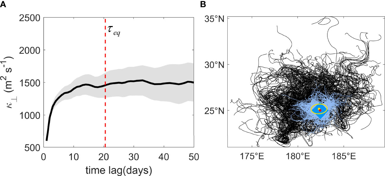
Figure 1 An illustration of the diagnosis procedure of ${\kappa }_{\perp }^{\infty }(x,L^{*})$ [Section 2.3, Eqs. (1) and (2)] and the scale-dependent mixing (SDM) nonlocality ellipse (Section 3.1). Here the adaptive bin is centered at (${182.45}^{\text{o}}\text{E}$, ${25.00}^{\text{o}}\text{N}$ ) and $L^{*}=1^{\circ }$. (A) The change of ${\kappa }_{\perp }(x,\tau ,L^{*})$ [Eq. (2), black solid line] with $\tau$ (the abscissa). ${\kappa }_{\perp }$ levels off at the equilibration time ${\tau }_{eq}$ (red vertical line). The gray shaded area indicates uncertainties at the 95% confidence level. (B) Sample pseudo-trajectories passing the adaptive bin centered at x (red dot), indicated by dark blue. Only 10% of the pseudo-trajectories are shown here to make these tracks visible. The light blue tracks represent the effective trajectories, corresponding to $\tau <{\tau }_{eq}$. The remaining part of the pseudo-trajectories is indicated by black. The yellow ellipse is the SDM nonlocality ellipse centered on the track centroid (yellow dot), inferred from the effective trajectories.

To determine the scale-dependent equilibration time (${\tau }_{eq}$), we first calculate the scale-dependent eddy diffusivity, i.e., the diffusivity induced by eddies smaller than the separation scale $L^{*}$. We consider $L^{*}$ ranging from ${0.2}^{\circ }$ to ${2.5}^{\circ }$ ($\approx$ 22-275 km). The Lagrangian formula for scale-dependent eddy diffusivity has an analogous form to that of total eddy diffusivity (e.g., Griesel et al., 2010; Chen et al., 2014). As shown in Liu et al. (2023), the scale-dependent cross-stream eddy diffusivity ${\kappa }_{\perp }^{\infty }(x,L^{*})$ can be diagnosed from

$\begin{array}{ll}{\kappa }_{\perp }^{\infty }(x,L^{*})=\underset{\tau \to \infty }{\lim }{\kappa }_{\perp }(x,\tau ,L^{*})\approx \frac{{\displaystyle {\int }_{{\tau }_1}^{{\tau }_2}{\kappa }_{\perp }(x,\tilde{\tau },L^{*})d\tilde{\tau }}}{{\tau }_2-{\tau }_1},& (1)\end{array}$

where

$\begin{array}{ll}{\kappa }_{\perp }(x,\tau ,L^{*})={\displaystyle {\int }_0^{\tau }d\tilde{\tau }\langle u_{\perp }^{\text{'}}(t_0|x,t_0)u_{\perp }^{\text{'}}(t_0+\tilde{\tau }|x,t_0)\rangle .}& (2)\end{array}$

Equations (1) and (2) can be rigorously derived using the Green’s function method and based on the scale separation assumption. For details of the derivation, see Supporting Information of Liu et al. (2023). Their derivation reveals that when diagnosing scale-dependent eddy diffusivity, particles need to be advected by the total flow field, not just by total eddy velocity or scale-dependent eddy velocity. Note that previous studies have demonstrated that total eddy diffusivity is also inferred from particle trajectories advected by the total flow velocity (e.g., Davis, 1991; LaCasce, 2008; Chen et al., 2014; Van Sebille et al., 2018). Therefore, the requirement of particle advection by total velocity for scale-dependent eddy mixing here is consistent with the total mixing case in literature.

In Eq. (2) above, $u_{\perp }^{\text{'}}(t_0+\tilde{\tau }|x,t_0)$ is the scale-dependent cross-stream eddy velocity at time $t_0+\tilde{\tau }$ for the particle that passes location $x$ at time $t_0$. Cross-stream direction is the direction perpendicular to the mean flow. Note that different from Chen et al. (2014), $u_{\perp }^{\text{'}}$ in this study denotes the scale-dependent, not total, eddy velocity in the cross-stream direction. These scale-dependent eddy velocity is obtained through spatially filtering the total eddy velocity. As an example, Figure S1 in Supplementary Materials shows snapshots of scale-dependent meridional velocity. $\langle ·\rangle$ represents averaging over all the particles in the bin centered at $x$. We use pseudo-trajectories, generated from the original particle trajectories, and adaptive bins to obtain converged eddy diffusivity. This approach have been proven effective in estimating converged eddy diffusivity at high spatial resolution (Koszalka and LaCasce, 2010; Klocker et al., 2012; Chen et al., 2014).

As shown in Figure 1A, when $\tau$ reaches the Lagrangian equilibration time ${\tau }_{eq}$ (Figure 1A, red line), the particle velocity decorrelates from its initial velocity, and ${\kappa }_{\perp }(x,\tau ,L^{*})$ levels off. This phenomenon is called the convergence of ${\kappa }_{\perp }(x,\tau ,L^{*})$, and the converged value is considered to be the scale-dependent eddy diffusivity ${\kappa }_{\perp }^{\infty }(x,L^{*})$. In practice, we chose $[{\tau }_1,{\tau }_2]$ to be $[{\tau }_{eq}-15,{\tau }_{eq}+15]$ days. For further details of estimating Lagrangian equilibration time ${\tau }_{eq}$, see Chen et al. (2014) and Chen and Waterman (2017). Note that for some adaptive bins, the Lagrangian autocorrelation function from Eq. (2) has a negative lobe following the positive lobe (e.g., Figure S2 in Supplementary Material). This negative lobe can lead to a decrease of eddy diffusivity (Figure S2B). We found that using our criteria about the ${\tau }_{eq}$ diagnosis, we have already included the effect of negative lobes on the eddy diffusivity magnitude. This is because ${\tau }_{eq}$ denotes the earliest time when ${\kappa }_{\perp }$ levels off over a 30-day time period, not the time of the first zero-crossing where the negative lobe starts. Over the time-lag range with the negative lobe, ${\kappa }_{\perp }$ generally has not yet converged, i.e., leveled off. In other words, the Lagrangian equilibration time ${\tau }_{eq}$, based on our criteria, is generally no smaller than the timelag where the negative lobe locates (e.g., Figure S2B).

Concerning convergence, the percentage of adaptive bins with converged ${\kappa }_{\perp }$ ranges from 99.86-100% for all $L^{*}$. Specifically, the diffusivity in all bins can reach convergence for $L^{*}$ ranging from ${0.2}^{\circ }$ to ${1.8}^{\circ }$. For $L^{*}=2^{\circ }$ and ${2.5}^{\circ }$, only one of the adaptive bins does not have converged eddy diffusivity. This high convergence rate is partially attributed to the sufficient numerical particles we deployed. The usage of pseudo-trajectories and the adaptive bin clustering method also contributes to the high convergence rate (Chen et al., 2014). First, for each particle trajectory, we consider the particle positions every 3 days as a new starting point. Then, we track the particle forward for 115 days from the new starting point to obtain a new trajectory, which is termed a pseudo-trajectory. Through repeating this procedure, we obtain many pseudo-trajectories from one original particle trajectory. This method help convert tens of thousands of original trajectories to millions of pseudo-trajectories. Two, Eq. (2) is the ensemble average of the autocorrelation functions over all the pseudo-trajectories passing through a chosen finite area. The number of pseudo tracks passing each geographic bin can vary greatly because of the flow inhomogeneity, leading to a low convergence rate of diffusivity (Chen et al., 2014). In contrast, adaptive bins, with irregular shapes and spatially varying sizes, can ensure that the number of pseudo-trajectories in each bin is roughly the same, leading to improved convergence rate (Chen et al., 2014). We divide the KE region into a number of adaptive bins, using the K-means clustering algorithm and the starting points of these pseudo-trajectories (Koszalka and LaCasce, 2010; Chen et al., 2014).

Particle trajectories in the time range $\tau <{\tau }_{eq}$ are considered to be effective trajectories (Figure 1B, light blue area). Note that diagnosing eddy diffusivity for an adaptive bin requires the information of all the effective trajectories, which covers a larger area than the adaptive bin itself (Figure 1B, dark blue area). This indicates that, similar to Eulerian eddy diffusivity, Lagrangian eddy mixing is essentially a non-local concept.

3 Nonlocality of scale-dependent mixing: estimation

3.1 Nonlocality ellipse

The area enclosing these effective trajectories can indicate the degree of mixing nonlocality (Figure 1B, light blue area). However, this area generally has an irregular shape, making it challenging to depict the basic characteristics of mixing nonlocality. To address this issue, Chen and Waterman (2017) introduced the concept of nonlocality ellipse to quantify the TM nonlocality based on effective trajectories. Inspired by this study, to quantify the SDM nonlocality, we introduce the concept of the SDM nonlocality ellipse (Figure 2A). Specifically, the squares of the semimajor axis length (${\sigma }_{1,n}$) and the semiminor axis length (${\sigma }_{2,n}$) of the SDM nonlocality ellipse can be quantified as follows,

FIGURE 2

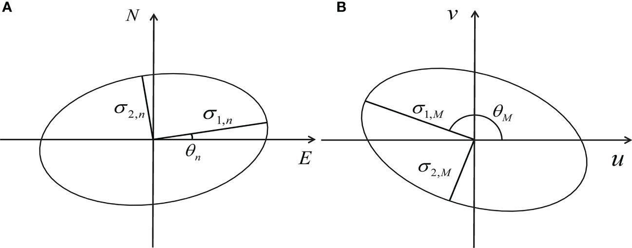
Figure 2 (A) The scale-dependent mixing (SDM) nonlocality ellipse with the centroid locating at (${182.45}^{\text{o}}\text{E}$, ${25.00}^{\text{o}}\text{N}$), i.e., the yellow ellipse in Figure 1B. (B) The momentum ellipse with the centroid locating at (${182.40}^{o}E$, ${25.00}^{\text{o}}\text{N}$). The semimajor axis length ${\sigma }_{1,n}$, semiminor axis length ${\sigma }_{2,n}$ and tilt ${\theta }_n$ of the SDM nonlocality ellipse are respectively defined in Eqs. (3), (4) and (6), while those for the momentum ellipse (${\sigma }_{1,M}$, ${\sigma }_{2,M}$ and ${\theta }_M$) are defined in Eqs. (14)-(16).

$\begin{array}{ll}{\sigma }_{1,n}^2=\frac{1}{2}[{\sigma }_x^2+{\sigma }_y^2+\sqrt{{({\sigma }_x^2-{\sigma }_y^2)}^2+4{({\sigma }_{xy}^2)}^2}],& (3)\end{array}$

$\begin{array}{ll}{\sigma }_{2,n}^2=({\sigma }_x^2+{\sigma }_y^2)-{\sigma }_{1,n}^2,& (4)\end{array}$

where

$\begin{array}{ll}\{\begin{array}{l}{\sigma }_x^2=\frac{{\displaystyle {\int }_0^{{\tau }_{eq}}{\displaystyle {\sum }_{i=1}^N{[x_i(t)-x_c]}^{2}dt}}}{N{\tau }_{eq}},\hfill \\ {\sigma }_y^2=\frac{{\displaystyle {\int }_0^{{\tau }_{eq}}{\displaystyle {\sum }_{i=1}^N{[y_i(t)-y_c]}^{2}dt}}}{N{\tau }_{eq}},\hfill \\ {\sigma }_{xy}^2=\frac{{\displaystyle {\int }_0^{{\tau }_{eq}}{\displaystyle {\sum }_{i=1}^N[x_i(t)-x_c][y_i(t)-y_c]dt}}}{N{\tau }_{eq}}.\hfill \end{array}& (5)\end{array}$

Here ${\sigma }_x^2$, ${\sigma }_y^2$ and ${\sigma }_{xy}^2$ respectively represent the zonal, meridional and cross variance of each particle position on the effective trajectory relative to the track centroid. These effective trajectories are for the scale-dependent eddy mixing (Section 2.3). ($x_i$, $y_i$) denotes the particle position on the effective trajectory at the $i_{th}$ time. ($x_c$, $y_c$) is the track centroid, which is the average of all particle positions of effective trajectories in an adaptive bin. $N$ is the total number of these particle positions.

Following Chen and Waterman (2017), we chose to remap the converged diffusivity values and the nonlocality ellipse center from the adaptive bin centroid [$x$ in Eq. (2), red dot in Figure 1B] to the track centroid [($x_c$, $y_c$), yellow dot in Figure 1B]. Our rationale is as follows. The nonlocality ellipse is inferred from effective trajectories. As stated in section 2.3, the adaptive bin is composed of the geographic location of the starting points of pseudo-trajectories (dark blue area in Figure 1B). However, as $\tau$ increases, particles for these trajectories gradually drift away from the bin centroid, and thus the effective trajectories, used to diagnose diffusivity for each bin, could cover a larger area than the bin itself. As a result, these diffusivity estimates are essentially nonlocal, representing mixing in the area covered by the effective trajectories centered at the track centroid. Therefore, the track centroid can better represent the spatial location of the diffusivity and its nonlocality estimates than the bin centroid (Chen and Waterman, 2017).

The tilt ${\theta }_n$ (Figure 2A) and the eccentricity $E_n$ respectively represents the orientation and anisotropy of the SDM nonlocality ellipses,

$\begin{array}{ll}{\theta }_n=\arctan (\frac{{\sigma }_{1,n}^2-{\sigma }_x^2}{{\sigma }_{xy}^2}),{\theta }_n\in [-\frac{\pi }{2},\frac{\pi }{2}],& (6)\end{array}$

$\begin{array}{ll}{E}_n=\frac{{\sigma }_{1,n}^2-{\sigma }_{2,n}^2}{{\sigma }_{1,n}^2+{\sigma }_{2,n}^2}.& (7)\end{array}$

The metric $L_{n,particle}$ refers to the square root of the SDM nonlocality ellipse area,

$\begin{array}{ll}{L}_{n,particle}=\sqrt{\pi \sqrt{{\sigma }_{1,n}^2}\sqrt{{\sigma }_{2,n}^2}}.& (8)\end{array}$

In this study $L_{n,particle}$ is an important metric we use to quantify the degree of the SDM nonlocality. We estimate the spatial structure and magnitude of $L_{n,particle}$ in Section 3.2 and evaluate the predictability of $L_{n,particle}$ in Section 4. $L_{n,particle}$ measures the area of the effective trajectories for each bin, which often extend beyond the bin boundary. Since eddy diffusivity is calculated from velocity fields along these effective trajectories, with a characteristics length scale of $L_{n,particle}$, the $L_{n,particle}$ information is implicitly included in the eddy diffusivity formula [Eqs. (1) and (2)]. In other words, the value of eddy diffusivity from Eqs. (1) and (2) depends on flow field within a distance on the order of magnitude of $L_{n,particle}$.

3.2 Results

3.2.1 Description about SDM nonlocality

Using the method from Section 3.1, here we estimate the SDM nonlocality ellipses for the separation scale ($L^{*}$) ranging from ${0.2}^{\circ }-{2.5}^{\circ }$.

3.2.1.1 Spatial pattern

As shown in Figure 3, the area of the SDM nonlocality ellipses has noticeable magnitude in the entire KE region, indicating that the SDM nonlocality is prevalent. The spatial pattern of $L_{n,particle}$ is insensitive to $L^{*}$, though. For all the available $L^{*}$ values, the SDM nonlocality share the following features. One, larger nonlocality ellipses are mainly located within the KE jet, corresponding to larger magnitude of $L_{n,particle}$. Two, nonlocality ellipses are zonally elongated in the upstream KE jet, with semimajor axis much longer than semiminor axis. In contrast, in the downstream KE jet, as the jet flow weakens and eddies gets more energetic, numerical particles actively move in both meridional and zonal directions. Therefore, the length of the semiminor axis increases and gets closer to that of the semimajor axis. Three, in the upstream region with intense jet, the ellipses on the jet flanks tend to tilt toward the jet (e.g., around ${145}^{\text{o}}\text{E}$). This phenomenon is related to the cross variance ${\sigma }_{xy}^2$, which is positive (negative) on the southern (northern) side of the KE jet. Consistent with the insensitivity of the SDM mixing nonlocality to $L^{*}$, the SDM nonlocality features summarized above resemble those of the TM nonlocality, which has been previously reported (Chen and Waterman, 2017; Guan et al., 2022).

FIGURE 3

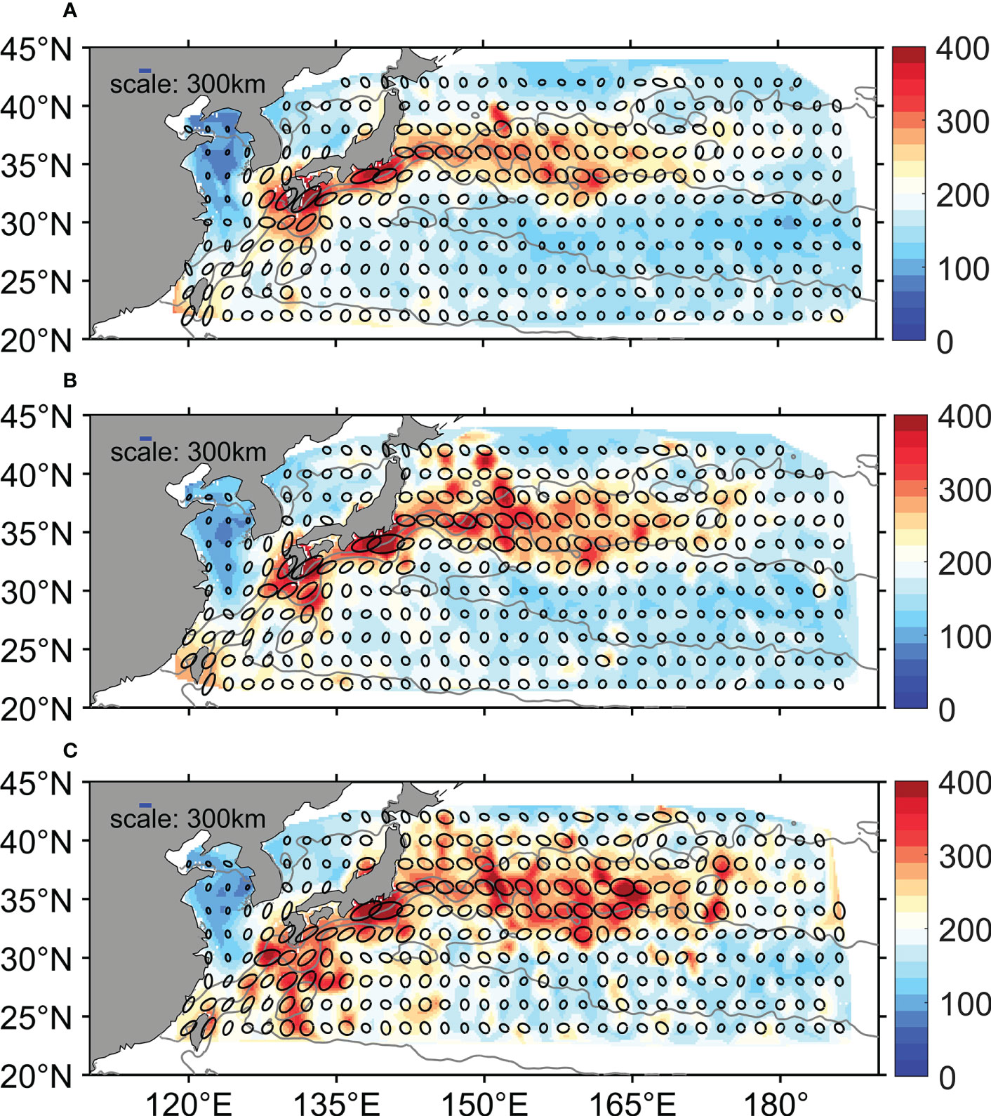
Figure 3 The scale-dependent mixing (SDM) nonlocality ellipse (black contours) and $L_{n,particle}$ in km [color, Eq. (8)] for the annual-mean scale-dependent cross-stream eddy diffusivity in the KE region. (A) $L^{*}={0.2}^{\circ }$, (B) $L^{*}=1^{\circ }$,and (C) $L^{*}={2.5}^{\circ }$. The blue horizontal line represents the scale of the SDM nonlocality ellipses in each panel. Gray contours are the barotropic streamlines defined as $g{f}^{-1}\overline{\eta }$ (Chen et al., 2014), where $g$ is the gravitational acceleration, $f$ denotes the Coriolis parameter, and $\overline{\eta }$ is the annual-mean sea surface height during 2011/09/13-2012/09/12.

3.2.1.2 Domain Averaged $L_{n,particle}$

The $L_{n,particle}$ magnitude is only weakly dependent on $L^{*}$. For example, as $L^{*}$ increases from ${0.2}^{\circ }$ to ${2.5}^{\circ }$, the domain-averaged $L_{n,particle}$ only increases from 182 to 213 km (Figure 4A). Considering that $L_{n,particle}$ is a metric closely linked with the Lagrangian equilibration time ${\tau }_{eq}$ (Section 3.1), the insensitivity of $L_{n,particle}$ to $L^{*}$ may be related to the weak dependence of ${\tau }_{eq}$ on $L^{*}$ (Figure 5). In addition, the fact that these particle trajectories are convoluted rather than straight further weakens the dependence of $L_{n,particle}$ on ${\tau }_{eq}$. Chen et al. (2014) found that in the KE region from a ${0.1}^{\circ }$ resolution model, the domain-averaged square root of the TM nonlocality ellipse area at all depth levels is less than 200 km. This number is on the same order of magnitude as $L_{n,particle}$ for $L^{*}={2.5}^{\circ }$ in our study.

FIGURE 4

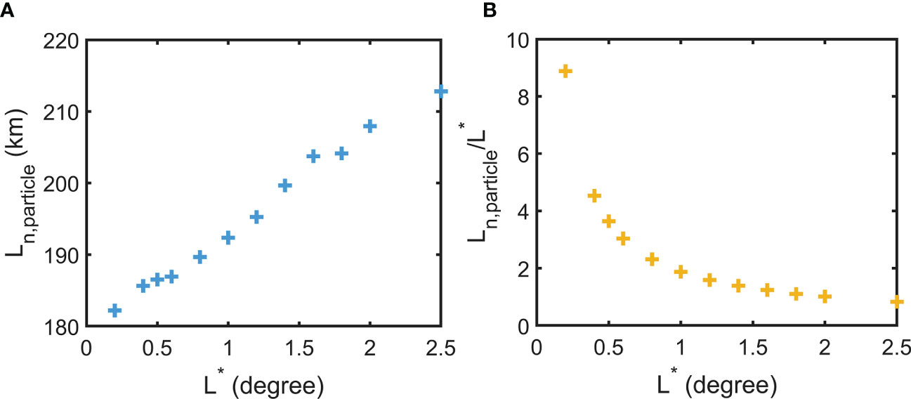
Figure 4 (A) Domain-averaged $L_{n,particle}$ for all the choices of $L^{*}$ we consider. (B) The ratio between the domain-averaged $L_{n,particle}$ and $L^{*}$.

FIGURE 5

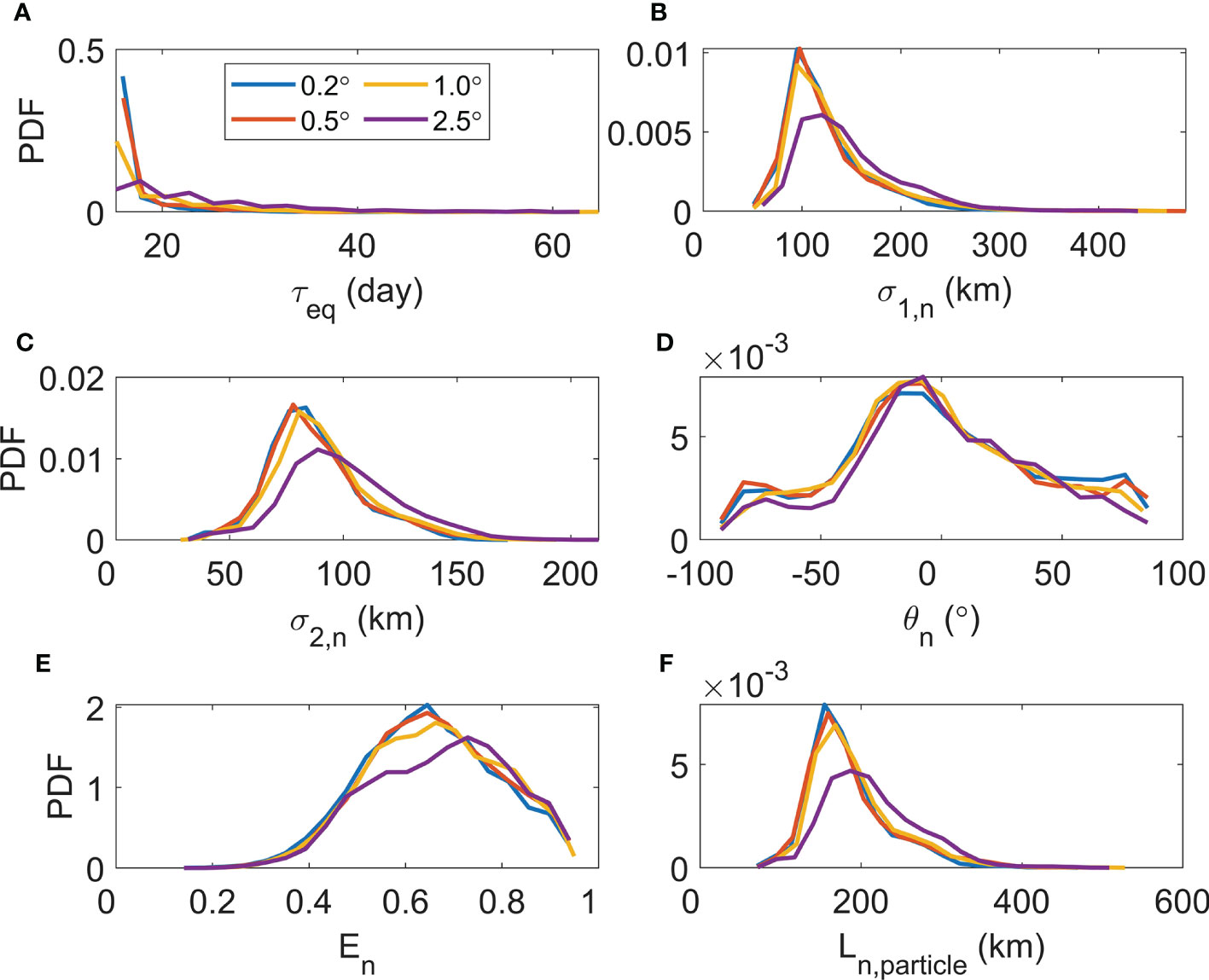
Figure 5 Probability density functions (PDFs) of the SDM nonlocality ellipse properties. (A) Equilibration time, ${\tau }_{eq}$ [Figure 1A], (B) semimajor axis length, ${\sigma }_{1,n}$ [Eq. (3)], (C) semiminor axis length, ${\sigma }_{2,n}$ [Eq. (4)], (D) tilt, ${\theta }_n$ [Eq. (6)], (E) eccentricity, $E_n$ [Eq. (7)], and (F) the degree of nonlocality, $L_{n,particle}$ [Eq. (8)]. The legend indicates the four cases we present here: $L^{*}={0.2}^{\circ }$, ${0.5}^{\circ }$, ${1.0}^{\circ }$, and ${2.5}^{\circ }$.

3.2.1.3 Nonlocality ellipse properties

To further assess the dependence of the nonlocality ellipse properties on $L^{*}$, we diagnosed their probability density functions (PDFs) (Figure 5). For all the available $L^{*}$, the PDF peak of the equilibration time ${\tau }_{eq}$ occurs at time shorter than 20 days. As $L^{*}$ increases, the PDF distribution of ${\tau }_{eq}$ shifts to longer days (Figure 5A). The PDFs for the semimajor axis length (${\sigma }_{1,n}$), semiminor axis length (${\sigma }_{2,n}$) and $L_{n,particle}$ share similar right-skewed distributions, consistent with those for the TM nonlocality [8,26]. When $L^{*}$ increases from ${0.2}^{\circ }$ to ${2.5}^{\circ }$, the PDFs of ${\sigma }_{1,n}$, ${\sigma }_{2,n}$ and $L_{n,particle}$ get lower and wider, especially for $L^{*}={2.5}^{\circ }$ (Figures 5B, C, F). For ${\sigma }_{1,n}$ (${\sigma }_{2,n}$), its value at the PDF peak increases from 95 (78) to 120 (89) km (Figures 5B, C) as $L^{*}$ increases. As to $L_{n,particle}$, its value at the PDF peak increases from 155 to 187 km (Figure 5F). The PDFs of the ellipse tilt (${\theta }_n$) are insensitive to the choice of $L^{*}$, with the peaks occurring at around $-8^{\circ }$ (Figure 5D). The PDF distribution of ${\theta }_n$ is consistent with that for the TM nonlocality (Chen and Waterman, 2017; Guan, 2022). Finally, similar to that of the TM nonlocality (Chen and Waterman, 2017; Guan, 2022), the PDF of the eccentricity ($E_n$) is left-skewed, ranging from 0.2 to1 (Figure 5E). As $L^{*}$ increases, the $E_n$ value at the PDF peak increases from 0.65 to 0.73.

Here we assess whether the spatial structures of these nonlocality ellipse properties are sensitive to the choice of $L^{*}$. We carried out the spatial correlation analysis between the nonlocality ellipse properties for $L^{*}={2.5}^{\circ }$ and those for other $L^{*}$ values ranging from ${0.2}^{\circ }-2^{\circ }$ (Figure 6). For the semimajor axis length, semiminor axis length, eccentricity and $L_{n,particle}$, the correlation coefficients are insensitive to the choice of $L^{*}$, with values ranging from 0.75 to 0.88. Therefore, for these four metrics, their spatial structures are only weakly dependent on the choice of $L^{*}$. However, the correlation value for ${\tau }_{eq}$ increases as $L^{*}$ increases. Its maximum, occurring at $L^{*}=2^{\circ }$, is only 0.44. As to the ellipse tilt ${\theta }_n$, the correlation values range from 0.38 to 0.59. Note that $L_{n,particle}$ is an important metric for one to assess the validity of the local assumption inherent in eddy parameterization schemes (Section 3.2.2). The insensitivity of $L_{n,particle}$ to $L^{*}$, shown in Figure 6, may potentially simplify this validity task.

FIGURE 6

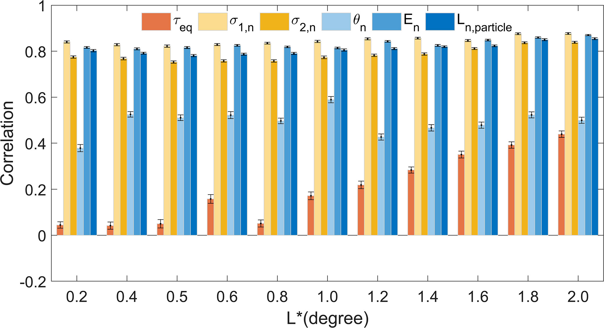
Figure 6 Spatial correlation coefficients of the SDM nonlocality ellipse properties between $L^{*}={2.5}^{\circ }$ and the other $L^{*}$ values ranging from ${0.2}^{\circ }-{2.0}^{\circ }$ (the abscissa). As indicated by the legend, these nonlocality ellipse properties are the same as those in Figure 5 [Figure 1A, Eqs. (3), (4), and (6)-(8)]. Error bars indicate uncertainties at the 95% confidence level based on a bootstrapping method (Chernick, 2011; Chen et al., 2014; Schulte et al., 2016; Ivanova et al., 2021).

3.2.2 The validity of the local mixing assumption

We estimated the ratio between the domain-averaged $L_{n,particle}$ and the domain-averaged $L^{*}$ (Figure 4B). Note that in practice, the separation scale $L^{*}$ can be interpreted as the resolvable scale of an ocean model or the oceanic component of a coupled model. For example, coarse-resolution climate models, e.g., the ocean component of the CMIP5 coupled models with $2^{\circ }$ resolution (Taylor et al., 2012), corresponds to relatively large $L^{*}$. In contrast, eddy-permitting (not eddy-resolving) models correspond to small $L^{*}$. Therefore, $L_{n,particle}/L^{*}$ can be used to assess whether the effect of mixing nonlocality needs to be included in eddy parameterization schemes. If $L_{n,particle}$ is larger than $L^{*}$, mixing nonlocality cannot be ignored. On the other hand, if $L^{*}$ is larger than $L_{n,particle}$, eddy mixing can be considered to be approximately local. In this case, the local assumption often used in existing eddy parameterization schemes (e.g., Gent and Mcwilliams, 1990; Ferrari and Nikurashin, 2010; Chen et al., 2015; Jansen et al., 2015; Wang and Stewart, 2020) are reasonable.

As shown in Figure 4B, as $L^{*}$ increases from ${0.2}^{\circ }$ to ${2.5}^{\circ }$, the ratio between the domain-averaged $L_{n,particle}$ and the domain-averaged $L^{*}$ decreases from 8.9 to 0.8. Assuming that this result is roughly valid across the entire ocean and for various climate scenarios, it would be reasonable to implement eddy parameterization schemes with the local assumption in coarse-resolution climate models, whose $L^{*}$ is relatively large (Redi, 1982; Liu et al., 2012; Jansen et al., 2015). red On the other hand, for the eddy-permitting models, the higher (smaller) the resolution ($L^{*}$), the more non-negligible mixing nonlocality is.

From a domain-average perspective, mixing nonlocality can be ignored in coarse-resolution climate models (Figure 4B). However, considering that mixing nonlocality has significant spatial variability (Figure 3), whether the local assumption holds depends on both $L^{*}$ and the geographical location. For example, $L_{n,particle}$ is smaller than 200 km in the area away from the KE jet, whereas it is larger than 300 km in the KE jet. This suggests that for a coarse-resolution model with $2^{\circ }$ resolution, the local assumption breaks down in the KE jet, but it still holds in the area away from the jet. Nevertheless, our findings show that both the magnitude and spatial pattern of $L_{n,particle}$ are relatively insensitive to $L^{*}$. This is a positive sign implying that it may be possible to develop a nonlocal parameterization scheme suitable for all $L^{*}$.

4 Nonlocality of scale-dependent mixing: representation and prediction

4.1 Method

Here we evaluate the skill of several methods in representing and predicting the SDM nonlocality, including the scaling method, curve-fitting method and RF. A schematic about the overall procedure is provided in Figure 7. The details of each method are provided next.

FIGURE 7

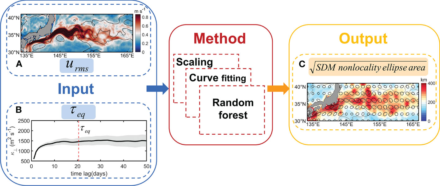
Figure 7 Schematic illustrating the procedure to represent and predict $L_{n,particle}$ using the scaling method, curve-fitting method and Random Forest (RF). The two input predictors are (A) total velocity magnitude ($u_{rms}$, $m{s}^{-1}$) and (B) the Lagrangian equilibration time for SDM (${\tau }_{eq}$, days). Example from (B) is ${\tau }_{eq}$ (red line) in the adaptive bin with centroid locating at (${182.45}^{\text{o}}\text{E}$, ${25.00}^{\text{o}}\text{N}$) for $L^{*}=1^{\circ }$(Figure 1A). The predictand is the square root of the SDM nonlocality ellipse area (km). As an example, panel (C) shows $L_{n,particle}$[Eq. (8)] for $L^{*}=1^{\circ }$(Figure 3B).

4.1.1 Scaling method

Considering that the nonlocality ellipse area essentially represents the spreading area of particles within the equilibration time, Chen and Waterman (2017) proposed a scaling method to represent the degree of the TM nonlocality. They considered that the square root of the TM nonlocality ellipse area can be represented by a linear function of ${\tau }_{eq,T}·u_{eddy}$, where ${\tau }_{eq,T}$ is the Lagrangian equilibration time for total mixing. The variable $u_{eddy}$ denotes the time mean of eddy velocity magnitude, i.e., $\sqrt{u^{\text{'}2}+v^{\text{'}2}}$, where $u$ and $v$ are zonal and meridional velocities and the prime denotes the deviation from its time mean. This linear empirical model, from Chen and Waterman (2017), is based on the assumption that the particle trajectories are straight lines. They found that this method can effectively represent the TM nonlocality.

Specifically, we express the square root of the SDM nonlocality ellipse area as follows

$\begin{array}{ll}{L}_{n,scaling}=a_0\sqrt{\pi {({\tau }_{eq}·u_{rms}/2)}^2}+b_0,& (9)\end{array}$

where $L_{n,scaling}$ measures the square root of the SDM nonlocality ellipse area based on the scaling method. Here ${\tau }_{eq}$ represents the Lagrangian equilibration time for scale-dependent eddy mixing. For any $L^{*}$, the Lagrangian particles are advected by the total flow. Therefore, in our scaling, instead of using eddy velocity magnitude, we chose to use the time-mean total velocity magnitude ($u_{rms}$); that is, the time mean $\sqrt{u^2+v^2}$ averaged over the time period of 2011/09/13 $\sim$ 2012/09/12. Here $u$ and $v$ are total velocity in the zonal and meridional directions. The variables $a_0$ and $b_0$ are obtained through linear least squares fitting between $\sqrt{\pi {({\tau }_{eq}·u_{rms}/2)}^2}$ and the particle-based estimate $L_{n,particle}$. Note that the coefficients $a_0$ and $b_0$ depend both on $L^{*}$ and on the dataset used for the least squares fitting.

4.1.2 Curve fitting method

Although the scaling method captures the link between $\sqrt{\pi {({\tau }_{eq}·u_{rms}/2)}^2}$ and the SDM nonlocality, this simple linear model may have relatively low accuracy. Given that the nonlinear curve-fitting approach proves useful in eddy mixing studies (e.g., Wang and Stewart, 2020), we employ this method to construct nonlinear functions between the $\sqrt{\pi {({\tau }_{eq}·u_{rms}/2)}^2}$ and $L_{n,particle}$. Through trial and error, we choose the complex function [Eq. (11)] and the quadratic function [Eq. (10)] to represent and predict $L_{n,particle}$,

$\begin{array}{ll}{L}_{n,fitting1}=a_1\sqrt{\pi {({\tau }_{eq}·u_{rms}/2)}^2}+b_1\log (\sqrt{\pi {({\tau }_{eq}·u_{rms}/2)}^2})+c_1,& (10)\end{array}$

$\begin{array}{ll}{L}_{n,fitting2}=a_2{(\sqrt{\pi {({\tau }_{eq}·u_{rms}/2)}^2})}^2+b_2\sqrt{\pi {({\tau }_{eq}·u_{rms}/2)}^2}+c_2,& (11)\end{array}$

where $L_{n,fitting1}$ denotes the represented/predicted value of the SDM nonlocality using the complex function, and $L_{n,fitting2}$ denotes those using the quadratic function. Their corresponding optimal fitting coefficients (i.e., $a_1$, $b_1$, $a_2$ and $b_2$) can be obtained through least squares fitting between $\sqrt{\pi {({\tau }_{eq}·u_{rms}/2)}^2}$ and the particle-based estimate $L_{n,particle}$. These coefficients depend on both $L^{*}$ and the dataset used for the least squares fitting.

4.1.3 Random forest

Although the curve-fitting method may be more accurate than the scaling method, identifying an appropriate fitting function and determining the optimal coefficients can be both challenging and time-consuming. In contrast, the RF method, which is a widely-used algorithm of machine learning (Ho, 1995), is computationally efficient with relatively few parameters and little configuration (Biau and Scornet, 2016; Li et al., 2016; Serras et al., 2019). RF can capture the complex nonlinear relation between the predictands and predictors, and can achieve high prediction accuracy. Therefore, it has been successfully applied in several oceanic and atmospheric prediction problems (e.g., Li et al., 2016; Gregor et al., 2017; Tong et al., 2019). RF has also been proven useful to predict the seasonal variability of total mixing lengths lengths (Guan et al., 2022) and the TM nonlocality in the KE region (Guan, 2022). Here we use the RF method to predict $L_{n,particle}$ using the two predictors: ${\tau }_{eq}$ and $u_{rms}$. For more details of RF, see Biau and Scornet (2016) and Breiman (2001).

We chose to use the RF code employed in several previous studies (e.g., Wang et al., 2016; Meng et al., 2018; Yadav et al., 2018; Liu et al., 2021; Guan et al., 2022), available at https://code.google.com/archive/p/randomforest-matlab/downloads. Our RF approach is expressed as

$\begin{array}{ll}{L}_{n,RF}=F({\tau }_{eq},u_{rms}),& (12)\end{array}$

where $L_{n,RF}$ represents the square root of the SDM nonlocality ellipse area from RF. The predictors (input) for the RF model are ${\tau }_{eq}$ and $u_{rms}$, and the predictand (output) is $L_{n,particle}$ (Figure 7). The dataset, including both predictors and predictand, can be split into a training dataset and a test dataset. $F$ denote the RF model constructed between the two input predictors and $L_{n,particle}$. This RF model changes with both $L^{*}$ and the amount of data used for training. Before running the RF model, a Z-score normalization is applied to the dataset. To test the representation and prediction skill of RF respectively, we carried out two types of experiments (schematic available in Figure S3 from Supplementary Materials). Here “representation skill” means the degree of fit of the training dataset, whereas “prediction skill” means the degree of fit of the testing dataset. Specifically, to assess the representative skill of RF, we use the entire dataset as the training dataset to train the RF model. Then $u_{rms}$ and ${\tau }_{eq}$ from the same training dataset is used as the input of the trained model. Comparing the corresponding output of the trained model ($L_{n,RF}$) with $L_{n,particle}$ reveals the RF representation skill. Concerning the evaluation of the RF prediction skill, following the approach from Guan et al. (2022), we randomly split the entire datasets into a training dataset and a testing dataset, which respectively account for a% and 1-a% of the entire dataset. The former is used to generate a trained RF model. Then using $u_{rms}$ and ${\tau }_{eq}$ from the testing dataset as the RF model input, we can obtain the corresponding $L_{n,RF}$, whose comparison with $L_{n,particle}$ from the testing dataset reveals the RF prediction skill. In this study, we evaluate the prediction skill of RF for the choice of a% ranging from 1% to 99%. For all available $L^{*}$, there are over 30,000 effective samples in the original dataset.

In analogy, to evaluate the prediction skill of the scaling and curve-fitting methods (Section 4.2.2), we use the approach similar to RF described above. Specifically, we use the randomly sampled training dataset, which is a% of the entire dataset, and the least squares fitting approach to determine the uncertain parameters $a_i$, $b_i$ and $c_i$ in the scaling and curve-fitting models [Eq. (9)-(11)]. With the trained model [Eq. (9)-(11)] and the predictors from the remaining dataset, one can obtain the predictand $L_{n,scaling}$, $L_{n,fitting1}$ and $L_{n,fitting2}$. Comparing these predictand values with the corresponding $L_{n,particle}$ reveals the prediction skill of the scaling and curve-fitting models. Similarly, to obtain the representation skill of the scaling and curve-fitting methods, we use the entire dataset for training and then compared the trained values with $L_{n,particle}$ (Section 4.2.1).

4.2 Results

4.2.1 Representation skill

We compare the degree of the SDM nonlocality inferred from the particles (Figure 3) with that based on the three methods (Figures 8A, B, C). All the three methods (scaling, curve-fitting and RF methods) can well represent the spatial structure of $L_{n,particle}$. For example, large nonlocality mainly occurs within the KE jet (Figures 8A–C). We also quantified the error of these three methods in representing $L_{n,particle}$ (Figures 8D–F). The absolute difference between $L_{n,RF}$ and $L_{n,particle}$ is overall the smallest, with most values smaller than 30 km (Figure 8F). In contrast, both $\left|L_{n,scaling}-L_{n,particle}\right|$ and $\left|L_{n,fitting1}-L_{n,particle}\right|$ are large in the coastal regions, upstream KE jet and the topographic regions (e.g., Japan island, Shatsky Rise and Emperor Seamounts) (Figures 8D, E). Results for $L_{n,fitting2}$ are similar to those of $L_{n,fitting1}$ (not shown). The findings described above are insensitive to the choice of $L^{*}$. RF outperforms the scaling and curve-fitting methods for all the $L^{*}$ we consider.

FIGURE 8

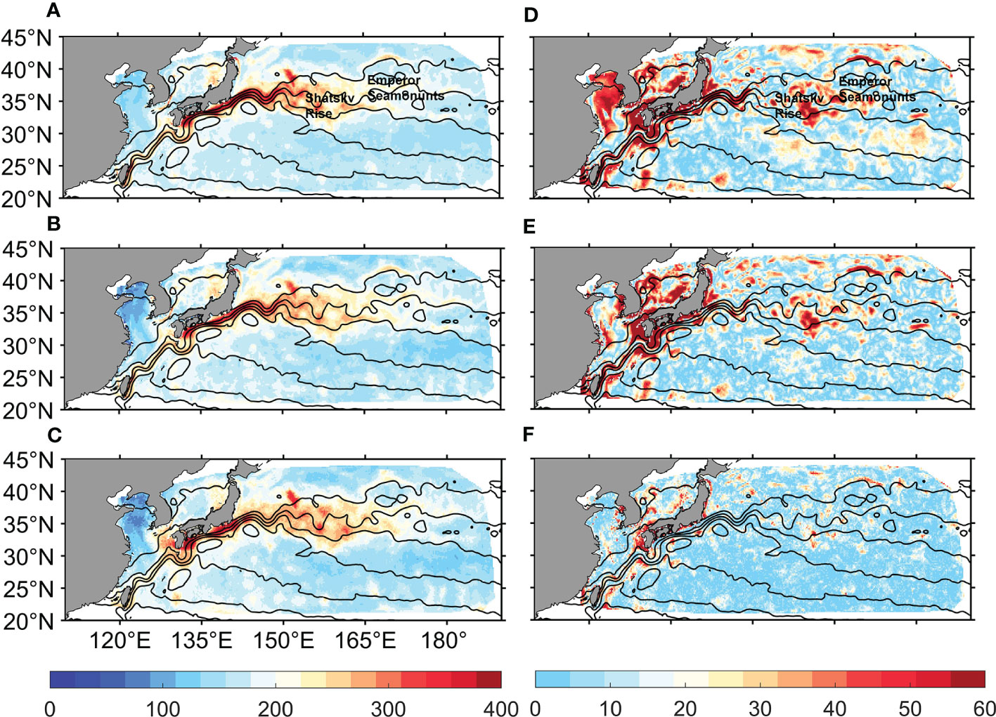
Figure 8 The degree of the SDM nonlocality from the scaling, curve-fitting and RF methods (A-C), and the corresponding absolute error (D-F). Results shown here are for $L^{*}={0.2}^{\circ }$. Spatial distribution of (A) $L_{n,scaling}$ [Eq.(9)], (B) $L_{n,fitting1}$ [Eq.(10)], (C) $L_{n,RF}$ [Eq.(12)], (D) $\left|L_{n,scaling}-L_{n,particle}\right|$, (E) $\left|L_{n,fitting1}-L_{n,particle}\right|$ and (F) $\left|L_{n,RF}-L_{n,particle}\right|$ in km. Here $L_{n,particle}$ is the particle-based SDM nonlocality [Eq.(8)]. Color bars on the left (right) are for the left (right) panels. The black lines are the barotropic streamlines as those in Figure 3. The topographic features “Shatsky Rise” and “Emperor Seamounts” are indicated in (A) and (D).

Concerning the large representation errors for $L_{n,scaling}$and $L_{n,fitting1}$ in several spots (e.g., coastal and topographic regions), we hypothesize that the large error may be related to the large spatial variability of the flow field. Note that both the scaling and curve-fitting approaches are essentially based on a single variable [i.e., $\sqrt{\pi {({\tau }_{eq}·u_{rms}/2)}^2}$]. Thus, these two methods roughly assume that particles are advected by a constant speed $u_{rms}$. This assumption apparently breaks down in the regions where the flow field changes direction abruptly (e.g., coastal regions, Japan island, Shatsky Rise and Emperor Seamounts). In these areas, particle trajectories are highly convoluted. Thus, using ${\tau }_{eq}$ and $u_{rms}$ as two separate predictors and constructing more complex predicting models, like RF, reduces the representation errors.

We calculated the correlation coefficient between $L_{n,particle}$ and the degree of nonlocality predicted by the three methods (Figure 9A). RF captures the spatial pattern of $L_{n,particle}$ much better than curve-fitting and scaling methods, with correlation coefficients larger than 0.96 for all the available $L^{*}$(Figure 9A). The two curve-fitting functions [Eqs. (10), (11)] have similar representation skills, with correlation values of nearly 0.85 for all the $L^{*}$ values. In contrast, the scaling method is overall inferior to the other methods, with correlation values within the range of [0.81, 0.84]. Despite such difference, all these methods have correlation values larger than 0.8. Therefore, all the three methods have reasonable skill in representing the spatial distribution of $L_{n,particle}$, with RF method being the best.

FIGURE 9

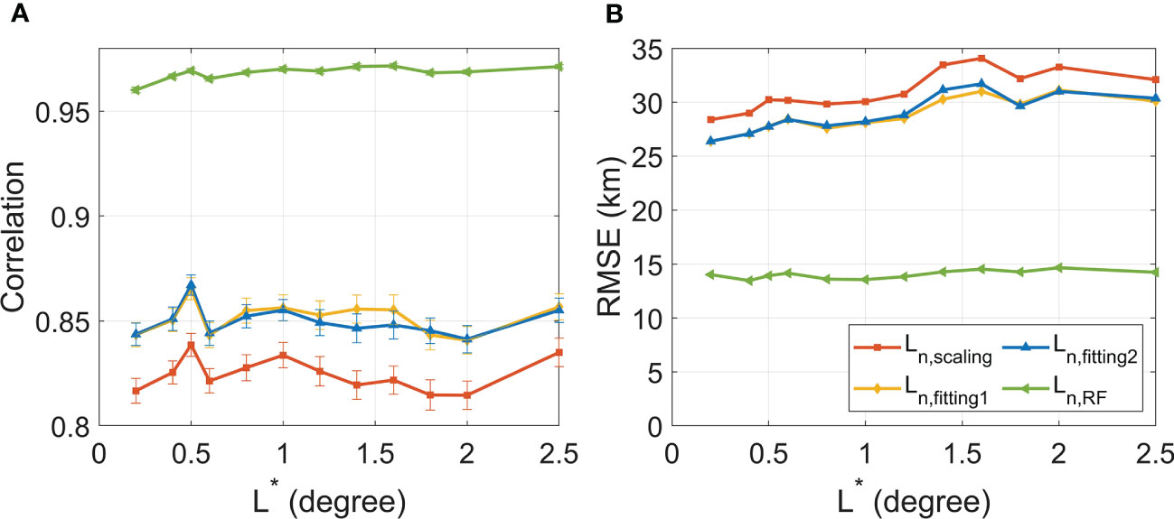
Figure 9 The skill of the scaling, curve-fitting and RF methods in representing the SDM nonlocality. (A) Correlation coefficients and (B) Root Mean Square Error (RMSE) between $L_{n,particle}$ and the degree of the SDM nonlocality based on each method as indicated at the legend. The horizontal axis L* (degree) means different separation scales. In the legend, $L_{n,scaling}$ represents the degree of the SDM nonlocality based on the scaling method [Eq. (9)], $L_{n,fitting1}$ and $L_{n,fitting2}$ are those based on the curve-fitting approach [Eqs. (10) and (11)], and $L_{n,RF}$ denotes that based on RF [Eq. (12)]. Error bars are uncertainties at the 95% confidence level using the bootstrapping method (Chernick, 2011; Chen et al., 2014; Schulte et al., 2016; Ivanova et al., 2021).

The Root Mean Square Error (RMSE) between the degree of nonlocality for each method and $L_{n,particle}$ (Figure 9B) indicates that RF also best captures the magnitude of $L_{n,particle}$. The ranking of these methods in representing the $L_{n,particle}$magnitude is consistent with their skill in capturing the spatial pattern (Figure 9B). RMSE for RF, ranging from 13.5 to 14.7, is much smaller than those of the scaling and curve-fitting methods, which are within the range of [26.4, 34.1]. The RMSE values for the two curve-fitting functions, which almost overlap with each other, are slightly smaller than those of the scaling method.

4.2.2 Prediction skill

Besides the representation skill, we also evaluate the skill of each method in predicting the SDM nonlocality (Figure 10). As described in Section 4.1.3, a randomly selected a% of the dataset is used to train the model (scaling, curve-fitting and RF) and the remaining dataset is used for the prediction skill evaluation. We estimate the RMSE and R-squared (the square of the correlation coefficients) between $L_{n,particle}$ and the corresponding predicted values (Figure 10). Among all the four methods, the RMSE (R-squared value) of RF is generally the smallest (largest), indicating that RF outperforms the other methods. For a given value of $L^{*}$, both RF and the curve-fitting methods outperform the scaling method for most choices of a%. The performance of the two curve-fitting functions are similar, better than scaling but only slightly inferior to RF. We also found that their prediction skills for large $L^{*}$ are better than those for small $L^{*}$. The R-squared and RMSE values are overall insensitive to the choice of a% within the range of [10%, 60%].

FIGURE 10

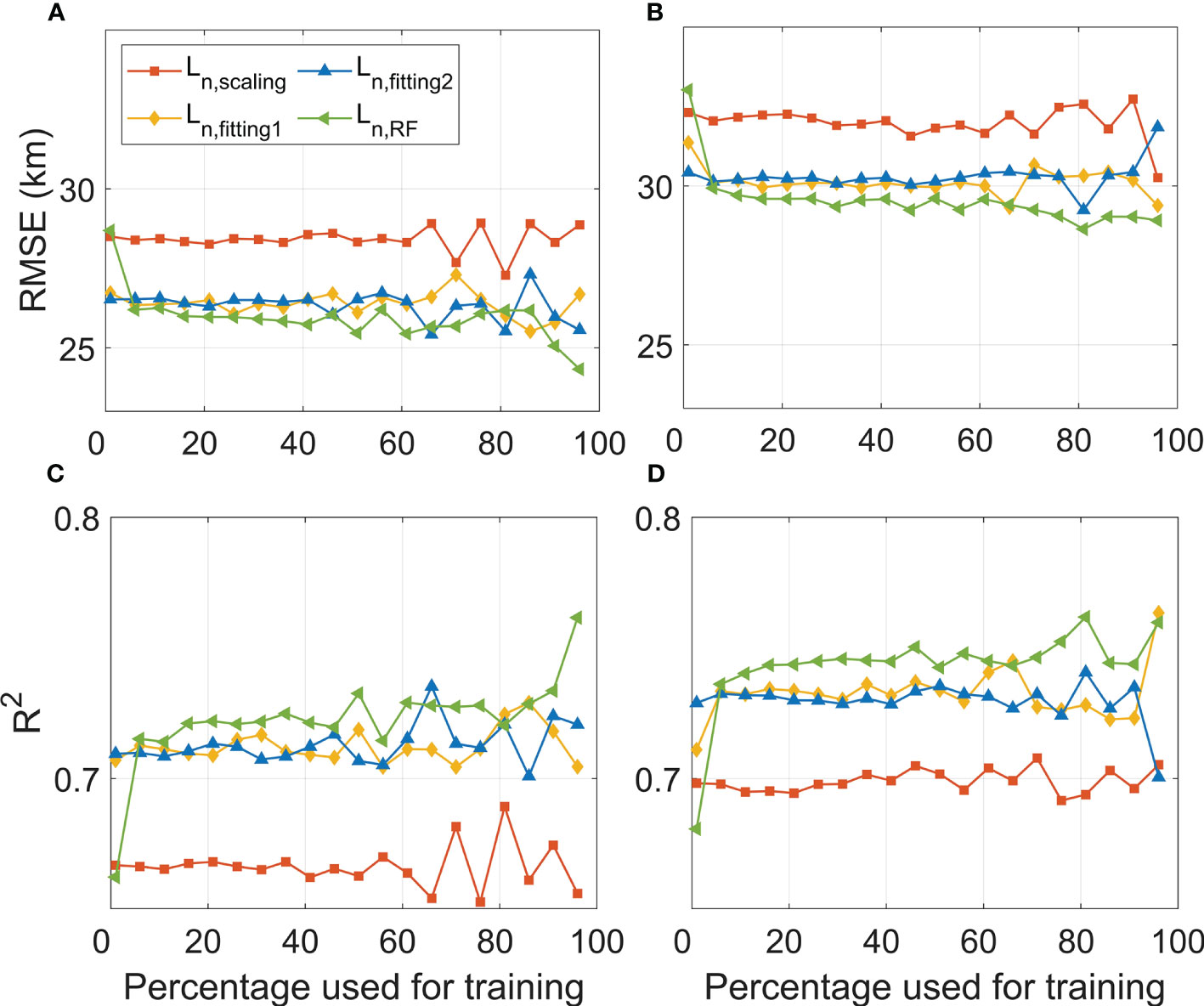
Figure 10 The skill of the scaling, curve-fitting and RF methods in predicting the SDM nonlocality. (A) RMSE, for $L^{*}={0.2}^{\circ }$, between $L_{n,particle}$ and the predicted counterparts based on each method. (B) is the same as (A) but for $L^{*}={2.5}^{\circ }$, (C) Correlation coefficients, for $L^{*}={0.2}^{\circ }$, between $L_{n,particle}$ and the predicted values, (D) is the same as (C) but for $L^{*}={2.5}^{\circ }$. The abscissa indicates the percentage of dataset used for the model training. The four terms in the legend apply for all the four panels. As stated in Figure 9, $L_{n,scaling}$ in the legend represents the degree of the SDM nonlocality based on the scaling method [Eq. (9)], $L_{n,fitting1}$ and $L_{n,fitting2}$ are those based on the curve-fitting approach [Eqs. (10) and (11)], and $L_{n,RF}$ denotes that based on RF [Eq. (12)].

Despite the significant advantage of RF in representing $L_{n,particle}$, the prediction skill of RF is only slightly superior to the curve-fitting methods (Figure 10). However, compared to the curve-fitting methods, one advantage of RF is that it can provide reasonable prediction while saving time and manpower. One might be able to further improve the performance of RF by further considering the underlying physics of SDM nonlocality and adding additional predictors.

5 Discussion

Although the SDM nonlocality can be reasonably estimated and predicted based on the information of Lagrangian particles (Sections 3 and 4), obtaining these particles are computationally expensive. Therefore, here we consider the possibility of representing $L_{n,particle}$ from the Eulerian perspective.

5.1 Momentum ellipses

5.1.1 Method

Chen and Waterman (2017) found that the particle-based TM nonlocality ellipse is closely related to the Eulerian momentum ellipse in an idealized barotropic quasigeostrophic model. Specifically, they found that in the regions with small nonlocality, the tilt and eccentricity of the TM nonlocality ellipses resemble those of the momentum ellipses. Guan (2022) extended their analysis to the realistic KE region using MITgcm llc4320 output. Guan (2022) found that in this realistic KE scenario, the area of the TM nonlocality ellipses is highly correlated with that of momentum ellipses. However, the tilt and eccentricity of the TM nonlocality ellipses match poorly with their counterparts in momentum ellipses.

Here we extend the comparison about mixing nonlocality and momentum ellipses to the scale-dependent context. Since the nonlocality ellipse for all $L^{*}$ is based on numerical particles advected by the total flow field, we mainly chose to compare the SDM nonlocality ellipse (Figure 2A) with the total momentum ellipse, i.e., the momentum ellipse inferred from total velocity fluxes (Figure 2B).

For the ease of comparison, in analogy to the definition of $L_{n,particle}$ , we define $L_M$ as the square root of the total momentum ellipse area,

$\begin{array}{ll}{L}_M=\sqrt{\pi \sqrt{{\sigma }_{1,M}^2}\sqrt{{\sigma }_{2,M}^2}},& (13)\end{array}$

where ${\sigma }_{1,M}$ and ${\sigma }_{2,M}$ denote the semimajor axis length and semiminor axis length of the total momentum ellipses (Figure 2B). We calculate them based on previous approach approach (Preisendorfer and Mobley, 1988; Waterman and Lilly, 2015; Chen and Waterman, 2017),

$\begin{array}{ll}{\sigma }_{1,M}^2=\frac{1}{2}[\overline{u^2}+\overline{v^2}+\sqrt{{(\overline{u^2}-\overline{v^2})}^2+4{(\overline{uv})}^2}],& (14)\end{array}$

$\begin{array}{ll}{\sigma }_{2,M}^2=\overline{u^2}+\overline{v^2}-{\sigma }_{1,M}^2.& (15)\end{array}$

Here $u$ and $v$ represent the zonally and meridionally total flow velocity, respectively. $\overline{·}$ represents the annual average (2011/09/13 to 2012/09/12). The tilt ${\theta }_M$ and the eccentricity $E_M$ of the total momentum ellipse can be calculated by

$\begin{array}{ll}{\theta }_M=\arctan (\frac{{\sigma }_{1,M}^2-\overline{u^2}}{\overline{uv}}),{\theta }_M\in [-\frac{\pi }{2},\frac{\pi }{2}],& (16)\end{array}$

$\begin{array}{ll}{E}_M=\frac{{\sigma }_{1,M}^2-{\sigma }_{2,M}^2}{{\sigma }_{1,M}^2+{\sigma }_{2,M}^2}.& (17)\end{array}$

For completeness, we also compare the SDM nonlocality ellipse with the scale-dependent momentum ellipse. One can then obtain the scale-dependent momentum ellipse using the formulas similar to the total momentum ellipse, simply replacing $u$ and $v$ from Eqs. (13)-(17) with $u_s$ and $v_s$. Here $u_s$ ($v_s$) refers to the component of zonal (meridional) velocity with scales smaller than $L^{*}$, obtained through spatial filtering.

5.1.2 Results

Figure S4(A) in Supplementary Materials shows the spatial pattern of the total momentum ellipse. We found that the spatial pattern of $L_M$ is similar to those of $L_{n,particle}$. For example, large values of $L_M$and $L_{n,particle}$ are mainly concentrated within the KE jet. To quantitatively compare the SDM nonlocality ellipse with the total momentum ellipse, we estimate the correlation of the ellipse properties between these two ellipses (Figure 11). Results are overall insensitive to the choice of $L^{*}$. The correlations of the square root of ellipse area are relatively high, ranging from 0.69 to 0.78 for the $L^{*}$ values we consider. The correlations about eccentricity and tilt are much lower, though. For eccentricity, they are no larger than 0.47, and for the tilt, they are around 0.1, with a maximum value of 0.16. Therefore, although the total momentum ellipse cannot well capture the eccentricity and tilt of the nonlocality ellipse, it can effectively represent the spatial distribution of $L_{n,particle}$. The disadvantage, however, is that the total momentum ellipse cannot directly predict the magnitude of $L_{n,particle}$.

FIGURE 11

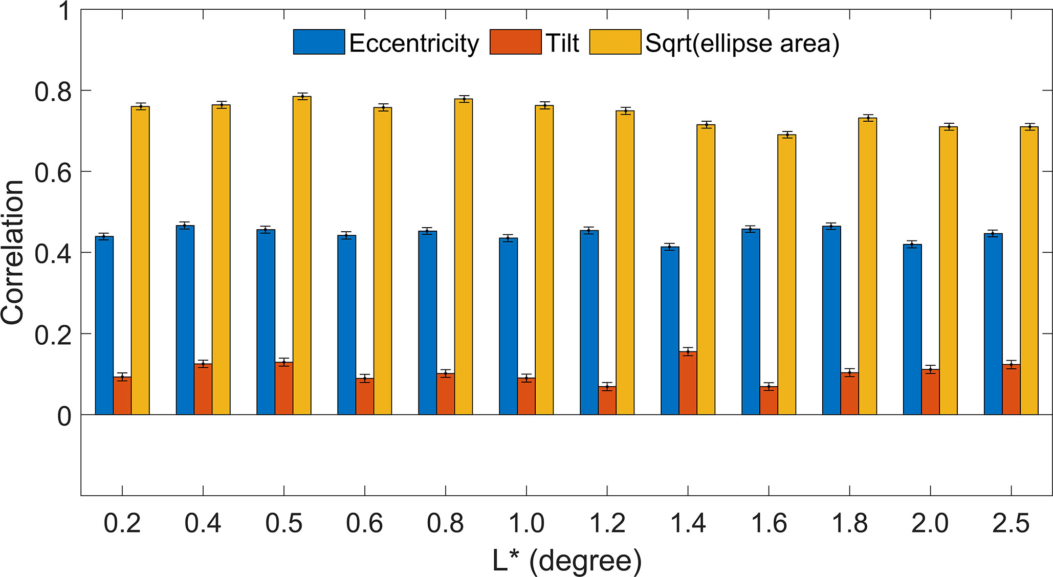
Figure 11 Spatial correlation coefficients of the ellipse properties, indicated on the legend, between the nonlocality ellipse and the momentum ellipse. In the legend, “Eccentricity’’ refers to $E_n$ [Eq. (7)] and $E_M$ [Eq. (17)], “Tilt’’ refers to ${\theta }_n$ [Eq. (6)] and ${\theta }_M$ [Eq. (16)], and “Sqrt (ellipse area)’’ represents $L_{n,particle}$ [Eq. (8)] and $L_M$ [Eq. (13)]. Error bars indicate uncertainties at the 95% confidence level based on a bootstrapping technique (Chernick, 2011; Chen et al., 2014; Schulte et al., 2016; Ivanova et al., 2021). The horizontal axis L* (degree) means different separation scales.

We also provide a comparison between the SDM nonlocality ellipse and the scale-dependent momentum ellipse (Figures S4 S5 in Supplementary Materials). The ellipse area decreases as $L^{*}$ decreases. Comparing Figure 11 with FigureS5 reveals that the area of the total momentum ellipse can better represent $L_{n,particle}$ than that of the scale-dependent momentum ellipse, especially for small $L^{*}$. This result is consistent with the fact numerical particles for the scale-dependent eddy mixing and its nonlocality diagnosis are advected by the total velocities, not scale-dependent ones [rationale available in Supporting Information from Liu et al. (2023)]. The degree of mixing non-locality is related to the area enclosing effective trajectories, which is thus closely linked with the total velocity and total momentum ellipse area.

5.2 Eulerian decorrelation approach

5.2.1 Method

$L_{n,particle}$ essentially represents the Lagrangian spatial decorrelation scale. Previous studies considered that there is a link between the Lagrangian decorrelation time scale ($T_L$) and the Eulerian decorrelation time scale ($T_E$) (Middleton, 1985; Chiswell et al., 2007; Chiswell and Rickard, 2008). Specifically, if particles pass through only a small portion of an eddy in the Eulerian decorrelation time (i.e., the eddy length scale is larger than the distance traveled by particles), $T_L\approx T_E$. This is because in this regime, the temporal decorrelation of Lagrangian velocity is mainly due to that of eddies. In contrast, if particles are fast advected through several eddies, the Lagrangian velocity reaches decorrelation more quickly and thus $T_L<T_E$. Given these previous findings, we hypothesize there might be a link between the Lagrangian and Eulerian decorrelation spatial scales. We assess whether the $L_{n,particle}$ can be represented by the Eulerian decorrelation spatial scale. If yes, one would be able to infer $L_{n,particle}$ directly from the Eulerian flow fields, without the need of calculating particle trajectories.

For this purpose, we need to estimate the Eulerian decorrelation spatial scale. Several methods have been proposed to diagnose the Eulerian decorrelation spatial scale (e.g, Cholemari and Arakeri, 2006; Chiswell et al., 2007). Here we propose the following simple method to estimate the Eulerian decorrelation spatial scale for scale-dependent mixing ($L_E$) (Figure 12). Specifically, we first estimate the autocorrelation between the time series (2011/09/13-2012/09/12) of the scale-dependent cross-stream eddy velocity [i.e., $u_{\perp }^{\text{'}}$ in Eq. (2)] at a given point and those at the surrounding points (Figure 12). Then we identify the points with significantly positive autocorrelation coefficients (Figure 12, black and gray dots). Finally, we estimate the area only including the given point and the connected identified points (Figure 12, black dots). $L_E$ is defined as the square root of the area covering these connected points.

FIGURE 12

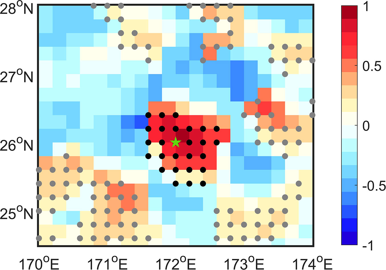
Figure 12 A schematic illustrating the procedure diagnosing the Eulerian decorrelation spatial scale $L_E$ (Section 5.2.1). Here we show the results of the scale-dependent cross-stream eddy velocity ($u_{\perp }^{\text{'}}$) for $L^{*}={2.5}^{\circ }$ as an example. Color represents the autocorrelations between $u_{\perp }^{\text{'}}$ at the initial center point (green pentagram) and those at the surrounding points. Dots indicate the gird points with significantly positive autocorrelation at the 95% confidence level. Among these dots, the black ones are the grid points which include the initial center point (green) and are spatially connected with each other. The gray dots represent the remaining points, which are disconnected with the black dots. The square root of the area covered by the black dots is the Eulerian decorrelation spatial scale $L_E$ for the initial center point.

5.2.2 Result and discussion

Comparing $L_E$with $L_{n,particle}$ reveals the skill of the Eulerian decorrelation approach in representing the SDM nonlocality. We found that $L_E$ differs much from $L_{n,particle}$ in the KE region. As shown in Figure 13), $\left|L_E-L_{n,particle}\right|$ is mostly below $2^{\circ }$ for $L^{*}={2.5}^{\circ }$. However, as $L^{*}$ decreases, $\left|L_E-L_{n,particle}\right|$ increases, especially within the KE jet. As shown in Figure 14A, the RMSE between $L_E$ and $L_{n,particle}$ increases from ${0.9}^{\circ }$ to ${1.56}^{\circ }$, as $L^{*}$ decreases from ${2.5}^{\circ }$ to ${0.2}^{\circ }$. Concerning the spatial correlation between $L_E$and $L_{n,particle}$, the correlation coefficient is statistically indistinguishable from zero for $L^{*}={0.2}^{\circ }$ and ${0.4}^{\circ }$. For $L^{*}>{0.4}^{\circ }$, the correlation coefficients are also small, with values no larger than 0.22 (Figure 14B). These low correlation values indicate that $L_E$poorly represents the spatial structure of $L_{n,particle}$.

FIGURE 13

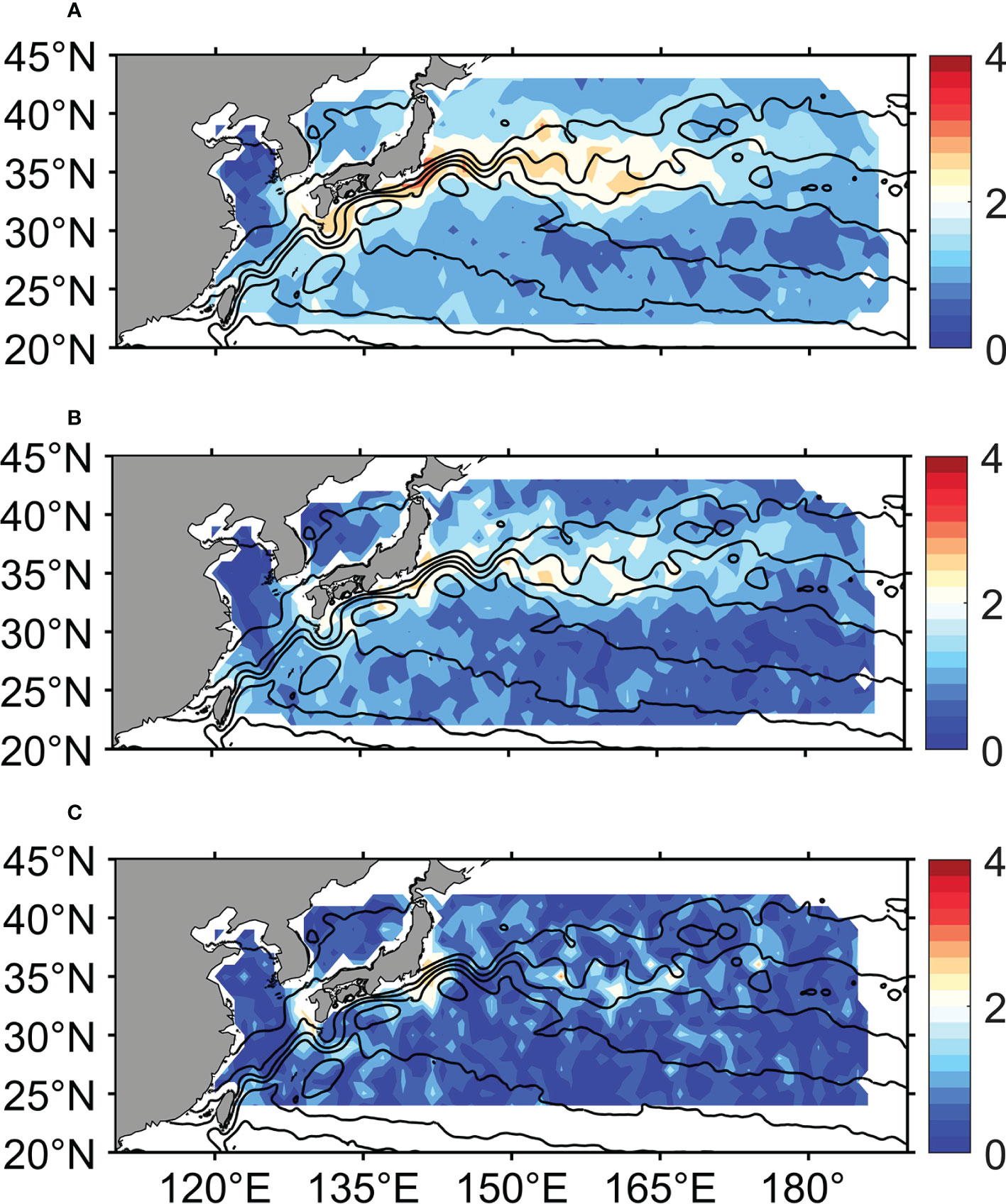
Figure 13 Spatial structure of $\left|L_E-L_{n,particle}\right|$ in degree for (A) $L^{*}={0.2}^{\circ }$, (B) $L^{*}=1^{\circ }$ and (C) $L^{*}={2.5}^{\circ }$. $L_E$denotes the Eulerian decorrelation spatial scale (Section 5.2.1) and $L_{n,particle}$ represents the degree of the SDM nonlocality [Eq. (8)].

FIGURE 14

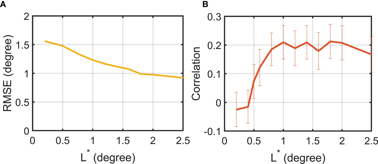
Figure 14 The (A) Root Mean Square Error (RMSE) (degree) and (B) the correlation coefficients between the Eulerian decorrelation spatial scale $L_E$ (Section 5.2.1) and the degree of the SDM nonlocality inferred from particles ($L_{n,particle}$) [Eq. (8)]. L* (degree) means the condition of different separation scales.

To summarize, despite its computational efficiency and ease of diagnosis, the Eulerian decorrelation approach is not ideal for the representation of SDM nonlocality. One, both $\left|L_E-L_{n,particle}\right|$ and RMSE increase as $L^{*}$ decreases (Figures 13, 14). However, as shown in Section 3.2.2, the effect of nonlocality becomes more significant as $L^{*}$ decreases. In other words, the error of $L_E$ in representing $L_{n,particle}$ is large for the range of $L^{*}$, where the SDM nonlocality cannot be ignored. Two, the large error is mainly concentrated within the KE jet (Figure 13). Yet, in this region, reasonable eddy parameterization scheme is crucial; because eddies there are rich and the SDM nonlocality is strong (Figure 3). Therefore, the Eulerian decorrelation method cannot replace the computationally expensive Lagrangian approach for the SDM nonlocality estimation.

The link between the Eulerian decorrelation scale and SDM nonlocality might be further investigated. First, the Eulerian decorrelation scale based on our approach essentially measures the square root of the area within the contour where the Eulerian correlation coefficient reaches their first zero-crossing over space. Yet, eddy diffusivity is obtained by integrating the Lagrangian autocorrelation function over the time lag range [0, ${\tau }_{eq}$]. The value of ${\tau }_{eq}$ generally differs from the first zero crossing of the Lagrangian autocorrelation. One may resolve this inconsistency by estimating a corresponding Eulerian decorrelation scale where the integral of the Eulerian autocorrelation function over space starts leveling off in the space coordinate. Further effort is left for future work. In addition, LaCasce (2008) has shown that the Eulerian decorrelation scale and the Lagrangian decorrelation scale can be linked through the ratio of the Eulerian integral time and advection time. Yet, no explicit analytical formula about this link has been provided. Further effort in this aspect might contribute to the prediction of mixing nonlocality based on tracer fields readily available in numerical models.

6 Summary

Motivated by the need to accurately parameterize subgrid eddy mixing processes in eddy-permitting climate models, here we estimate the degree of the SDM nonlocality ($L_{n,particle}$) in the KE region. We use the Lagrangian particle trajectories from the MITgcm llc4320 output to estimate $L_{n,particle}$. The spatial pattern of $L_{n,particle}$ is insensitive to $L^{*}$. Though $L_{n,particle}$ is noticeable in the entire study domain, its large values are mainly concentrated within the KE jet. Although $L_{n,particle}$ is only weakly dependent on $L^{*}$, the ratio between the domain averaged $L_{n,particle}$ and $L^{*}$ increases from 0.8 to 8.9 as $L^{*}$ decreases from ${2.5}^{\circ }$ to ${0.2}^{\circ }$. This suggests that the local assumption often inherent in eddy parameterization schemes roughly holds in coarse-resolution models. However, this assumption breaks down in models with relatively high resolution (e.g., the eddy-permitting, but not eddy-resolving ones). We also represent and predict $L_{n,particle}$ using the conventional scaling method, empirical curve-fitting method and a commonly used data-driven machine learning approach(RF). Among all these approaches, RF best represents and predicts both the spatial pattern and magnitude of $L_{n,particle}$. The curve-fitting method ranks second, and the scaling method has the worst performance. In particular, compared to the scaling and curve-fitting methods, RF has much better skill in representing the $L_{n,particle}$ magnitude in the coastal region and within the intense KE jet. The coastal region is critical for fisheries and human survival, whereas the KE jet plays a key role in modulating regional climate. Besides its reasonable performance, another advantage of RF is that it is less time consuming than the curve-fitting methods, which involve much trial and error searching the appropriate functions. However, caveats must be taken when choosing the predictors for RF. The choice of predictors needs to be based on the physical mechanism of the SDM nonlocality. For example, if we replace the total flow velocity magnitude by the scale-dependent eddy velocity magnitude as the input predictor in Section 4, the performance of RF gets relatively poor, especially for small values of $L^{*}$(not shown). This is because particles are advected by the total flow field, but not by the scale-dependent flow field.

This work can be further extended in several ways. One, we only consider the annual-mean SDM nonlocality using the MITgcm llc4320 output covering a relatively short time period (2011/09-2012/09). The seasonal or interannual variability of the SDM nonlocality remains unclear. Two, it would be worthwhile to revisit this problem in other ocean regions. Three, the approaches to estimate, represent and predict the SDM nonlocality needs to be further improved. The Lagrangian particle approach can provide the reasonable SDM nonlocality estimation and RF has reasonable skill in representing and predicting the SDM nonlocality. However, both methods require much information about the Lagrangian particles, which are not readily available in climate models. On the other hand, the momentum ellipse method can well represent the spatial pattern but not the magnitude of $L_{n,particle}$. As to the simple Eulerian decorrelation approach, its representation error is large especially for small $L^{*}$ and within the KE jet.

This study only considers eddy mixing nonlocality from a Lagrangian and time-mean perspective. Qian et al. (2019) has successfully demonstrated that in a transformed spatial coordinate related to quasi-conservative tracer contours, both Lagrangian single-particle diffusivity and relative diffusivity can be reconciled with the tracer-based effective diffusivity (Nakamura, 1996). This conceptual equivalence is valid from an instantaneous perspective. Since effective diffusivity represents eddy mixing across a specific tracer contour, it can be interpreted as eddy mixing averaged over each tracer contour. Whether the nonlocality of eddy mixing is noticeable and easily measurable in the context of the tracer-based effective diffusivity, in the transformed spatial coordinate or in the case of relative diffusivity is worth further theoretical consideration.

One limitation of this study is that we focus on estimating and predicting the degree of the SDM nonlocality, not developing eddy parameterization schemes including this nonlocality. Directly inferring realistic eddy mixing coefficients through data assimilation is an alternative approach towards improving eddy parameterization schemes. For example, Liu et al. (2012) has provided a novel approach to inferring eddy tracer mixing coefficients using an adjoint-based inversion model. They found that mixing coefficients from several existing schemes based on local parameters (e.g., Redi, 1982; Visbeck et al., 1997) need to be adjusted in order to obtain the best model-data fit. This approach from Liu et al. (2012) may offer further insights for developing and evaluating non-local eddy parameterization schemes. Our work has the following implications for improving eddy parameterization schemes. One, existing eddy parameterization schemes express eddy diffusivity as a function of local variables (e.g., Ferrari and Nikurashin, 2010; Mak et al., 2018; Wang and Stewart, 2020). Yet, our work indicates that eddy diffusivity could depend on both local variables and nonlocal variables in the surroundings areas within the distance of nonlocality scale. Future effort could be devoted to developing parameterization schemes expressing diffusivity as a function of both local and nonlocal parameters. Two, we found that as the separation scale $L^{*}$decreases, scale-dependent mixing is more nonlocal relative to $L^{*}$. Therefore, it is especially important to develop nonlocal parameterization schemes for eddy-permitting models. Three, the success of RF in predicting the SDM nonlocality suggests that employing appropriate machine learning methods may help estimate the nonlocality scale, which is key information for developing nonlocal eddy parameterization schemes.

Data availability statement

The original contributions presented in the study are included in the article/Supplementary Material. Further inquiries can be directed to the corresponding authors.

Author contributions

RC proposed and oversaw this project. ML analyzed the data and wrote the initial draft of the manuscript, which is revised by RC, WG, HZ, and TJ. WG also contributed by sharing expertise about total mixing and HZ by providing data support. All authors contributed to the article and approved the submitted version.

Funding

This study was funded by the National Natural Science Foundation of China (42076007).

Acknowledgments

We thank Glenn R. Flierl from Massachusetts Institute of Technology for helpful discussions on this work.

Conflict of interest

The authors declare that the research was conducted in the absence of any commercial or financial relationships that could be construed as a potential conflict of interest.

Publisher’s note

All claims expressed in this article are solely those of the authors and do not necessarily represent those of their affiliated organizations, or those of the publisher, the editors and the reviewers. Any product that may be evaluated in this article, or claim that may be made by its manufacturer, is not guaranteed or endorsed by the publisher.

Supplementary material

The Supplementary Material for this article can be found online at: https://www.frontiersin.org/articles/10.3389/fmars.2023.1137216/full#supplementary-material

References

Bachman S., Fox-Kemper B., Pearson B. (2017). A scale-aware subgrid model for quasi-geostrophic turbulence. J. Geophys. Res. 122, 1529–1554. doi: 10.1002/2016JC012265

CrossRef Full Text | Google Scholar

Biau G., Scornet E. (2016). A random forest guided tour. Test 25, 197–227. doi: 10.1007/s11749-016-0481-7

CrossRef Full Text | Google Scholar

Breiman L. (2001). Random forests. Mach. Learn. 45, 5–32. doi: 10.1023/A:1010933404324

CrossRef Full Text | Google Scholar

Brown A., Grant A. (1997). Non-local mixing of momentum in the convective boundary layer. Boundary-Layer Meteorol. 84, 1–22. doi: 10.1023/A:1000388830859

CrossRef Full Text | Google Scholar

Chen R., Gille S., McClean J. (2017). Isopycnal eddy mixing across the kuroshio extension: stable versus unstable states in an eddying model. J. Geophys. Res. 122, 4329–4345. doi: 10.1002/2016JC012164

CrossRef Full Text | Google Scholar

Chen R., Gille S., McClean J., Flierl G., Griesel A. (2015). A multiwavenumber theory for eddy diffusivities and its application to the southeast pacific (DIMES) region. J. Phys. Oceanogr. 45, 1877–1896. doi: 10.1175/JPO-D-14-0229.1

CrossRef Full Text | Google Scholar

Chen R., McClean J., T. G. S., Griesel A. (2014). Isopycnal eddy diffusivities and critical layers in the Kuroshio Extension from an eddying ocean model. J. Phys. Oceanogr. 44, 2191–2211. doi: 10.1175/JPO-D-13-0258.1

CrossRef Full Text | Google Scholar

Chen R., Waterman S. (2017). Mixing nonlocality and mixing anisotropy in an idealized western boundary current jet. J. Phys. Oceanogr. 47, 3015–3036. doi: 10.1175/JPO-D-17-0011.1

CrossRef Full Text | Google Scholar

Chen X., Xue M., Zhou B., Fang J., Zhang J. A., Marks F. D. (2021). Effect of scale-aware planetary boundary layer schemes on tropical cyclone intensification and structural changes in the gray zone. Monthly Weather Rev. 149, 2079–2095. doi: 10.1175/MWR-D-20-0297.1

CrossRef Full Text | Google Scholar

Chernick M. R. (2011). Bootstrap methods: a guide for practitioners and researchers (John Wiley & Sons).

Google Scholar

Chiswell S. M. (2013). Lagrangian Time scales and eddy diffusivity at 1000 m compared to the surface in the south pacific and Indian oceans. J. Phys. Oceanogr. 43, 2718–2732. doi: 10.1175/JPO-D-13-044.1

CrossRef Full Text | Google Scholar

Chiswell S., Rickard G. (2008). Eulerian and Lagrangian statistics in the bluelink numerical model and AVISO altimetry: validation of model eddy kinetics. J. Geophys. Res.: Oceans 113, C10024. doi: 10.1029/2007JC004673

CrossRef Full Text | Google Scholar

Chiswell S., Rickard G., Bowen M. (2007). Eulerian and Lagrangian eddy statistics of the Tasman Sea and southwest pacific ocean. J. Geophys. Res.: Oceans 112, C10004. doi: 10.1029/2007JC004110

CrossRef Full Text | Google Scholar

Cholemari M. R., Arakeri J. H. (2006). A model relating eulerian spatial and temporal velocity correlations. J. Fluid Mech. 551, 19–29. doi: 10.1017/S0022112005008074

CrossRef Full Text | Google Scholar

Davis R. (1987). Modeling eddy transport of passive tracers. J. Mar. Res. 45, 635–666. doi: 10.1357/002224087788326803

CrossRef Full Text | Google Scholar

Davis R. (1991). Observing the general circulation with floats. Deep-Sea Res. 38A (Suppl. 1), S531–S571. doi: 10.1016/S0198-0149(12)80023-9

CrossRef Full Text | Google Scholar

Eden C., Jochum M., Danabasoglu G. (2009). Effects of different closures for thickness diffusivity. Ocean Model. 26, 47–59. doi: 10.1016/j.ocemod.2008.08.004

CrossRef Full Text | Google Scholar

Ferrari R., Nikurashin M. (2010). Suppression of eddy diffusivity across jets in the southern ocean. J. Phys. Oceanogr. 40, 1501–1519. doi: 10.1175/2010JPO4278.1

CrossRef Full Text | Google Scholar

Ferrari R., Wunsch C. (2009). Ocean circulation kinetic energy: reservoirs, sources, and sinks. Annu. Rev. Fluid Mech. 41, 253–282. doi: 10.1146/annurev.fluid.40.111406.102139

CrossRef Full Text | Google Scholar

Frech M., Mahrt L. (1995). A two-scale mixing formulation for the atmospheric boundary layer. Boundary-layer meteorol. 73, 91–104. doi: 10.1007/BF00708931

CrossRef Full Text | Google Scholar

Gent P., Mcwilliams J. (1990). Isopycnal mixing in ocean circulation models. J. Phys. Oceanogr. 20, 150–155. doi: 10.1175/1520-0485(1990)020<0150:IMIOCM>2.0.CO;2

CrossRef Full Text | Google Scholar

Gnanadesikan A., Russell A., Pradal M.-A., Abernathey R. (2017). Impact of lateral mixing in the ocean on El nino in a suite of fully coupled climate models. J. Adv. Model. Earth Syst. 9, 2493–2513. doi: 10.1002/2017MS000917

CrossRef Full Text | Google Scholar

Gregor L., Kok S., Monteiro P. (2017). Empirical methods for the estimation of southern ocean CO 2: support vector and random forest regression. Biogeosciences 14, 5551–5569. doi: 10.5194/bg-14-5551-2017

CrossRef Full Text | Google Scholar

Griesel A., Gille S., Sprintall J., McClean J., LaCasce J., Maltrud M. (2010). Isopycnal diffusivities in the Antarctic circumpolar current inferred from Lagrangian floats in an eddying model. J. Geophys. Res. 115, C06006. doi: 10.1029/2009JC005821

CrossRef Full Text | Google Scholar

Griesel A., McClean J., Gille S., Sprintall J., Eden C. (2014). Eulerian and Lagrangian isopycnal eddy diffusivities in the southern ocean of an eddying model. J. Phys. Oceanogr. 44, 644–661. doi: 10.1175/JPO-D-13-039.1

CrossRef Full Text | Google Scholar

Guan W. (2022). Horizontal eddy mixing at the surface kuroshio extension: estimation and machine learning prediction (Tianjin University).

Google Scholar

Guan W., Chen R., Zhang H., Yang Y., Wei H. (2022). ). seasonal surface eddy mixing in the kuroshio extension: estimation and machine learning prediction. J. Geophys. Res. 127, e2021JC017967. doi: 10.1029/2021JC017967

CrossRef Full Text | Google Scholar

Hallberg R. (2013). Using a resolution function to regulate parameterizations of oceanic mesoscale eddy effects. Ocean Model. 72, 92–103. doi: 10.1016/j.ocemod.2013.08.007

CrossRef Full Text | Google Scholar

Ho T. K. (1995). “Random decision forests,” in Proceedings of 3rd international conference on document analysis and recognition (United States: IEEE), Vol. 1. 278–282. doi: 10.1109/ICDAR.1995.598994

CrossRef Full Text | Google Scholar

Hong S.-Y., Noh Y., Dudhia J. (2006). A new vertical diffusion package with an explicit treatment of entrainment processes. Monthly weather Rev. 134, 2318–2341. doi: 10.1175/MWR3199.1

CrossRef Full Text | Google Scholar

Inoue R., Harcourt R., Gregg M. (2010). Mixing rates across the gulf stream, part 2: implications for nonlocal parameterization of vertical fluxes in the surface boundary layers. J. Mar. Res. 68, 673–698. doi: 10.1357/002224011795977626

CrossRef Full Text | Google Scholar

Ivanova D. P., McClean J. L., Sprintall J., Chen R. (2021). The oceanic barrier layer in the Eastern Indian ocean as a predictor for rainfall over Indonesia and australia. geophys. Res. Lett. 48, e2021GL094519. doi: 10.1029/2021GL094519

CrossRef Full Text | Google Scholar

Jansen M., Adcroft A., Hallberg R., Held I. (2015). Parameterization of eddy fluxes based on a mesoscale energy budget. Ocean Model. 92, 28–41. doi: 10.1016/j.ocemod.2015.05.007

CrossRef Full Text | Google Scholar

Jansen M., Adcroft A., Khani S., Kong H. (2019). Toward an energetically consistent, resolution aware parameterization of ocean mesoscale eddies. J. Adv. Model. Earth Syst. 11, 2844–2860. doi: 10.1029/2019MS001750

CrossRef Full Text | Google Scholar

Jones C., Abernathey R. P. (2019). Isopycnal mixing controls deep ocean ventilation. Geophys. Res. Lett. 46, 13144–13151. doi: 10.1029/2019GL085208

CrossRef Full Text | Google Scholar

Klocker A., Abernathey R. (2014). Global patterns of mesoscale eddy properties and diffusivities. J. Phys. Oceanogr. 44, 1030–1046. doi: 10.1175/JPO-D-13-0159.1

CrossRef Full Text | Google Scholar

Klocker A., Ferrari R., LaCasce J., Merrifield S. (2012). Reconciling float–based and tracer–based estimates of lateral diffusivities. J. Mar. Res. 70, 569–602. doi: 10.1357/002224012805262743

CrossRef Full Text | Google Scholar

Koszalka I., LaCasce J. (2010). Lagrangian Analysis by clustering. Ocean dyna. 60, 957–972. doi: 10.1007/s10236-010-0306-2

CrossRef Full Text | Google Scholar

Kraichnan R. H. (1987). Eddy viscosity and diffusivity: exact formulas and approximations. Complex Syst. 1, 805–820.

Google Scholar

LaCasce J. (2008). Statistics from lagrangian observations. Prog. Oceanogr. 77, 1–29. doi: 10.1016/j.pocean.2008.02.002

CrossRef Full Text | Google Scholar

Large W., McWilliams J., Doney S. (1994). Oceanic vertical mixing: a review and a model with a nonlocal boundary layer parameterization. Rev. geophys. 32, 363–403. doi: 10.1029/94RG01872

CrossRef Full Text | Google Scholar

Li L., Schmitt R. W., Ummenhofer C. C., Karnauskas K. B. (2016). North Atlantic salinity as a predictor of sahel rainfall. Sci. Adv. 2, e1501588. doi: 10.1126/sciadv.150158

PubMed Abstract | CrossRef Full Text | Google Scholar

Liu M., Chen R., Flierl G. R., Guan W., Zhang H., Geng Q. (2023). Scale-dependent eddy diffusivities at the kuroshio extension: a particle-based estimate and comparison to theory. J. Phys. Oceanogr. In press. doi: 10.1175/JPO-D-22-0223.1

CrossRef Full Text | Google Scholar

Liu C., Köhl A., Stammer D. (2012). Adjoint-based estimation of eddy-induced tracer mixing parameters in the global ocean. J. Phys. Oceanogr. 42, 1186–1206. doi: 10.1175/JPO-D-11-0162.1

CrossRef Full Text | Google Scholar

Liu R., Wang Q., Zhang K., Wu H., Wang G., Cai W., et al. (2021). Analysis of postmortem intestinal microbiota successional patterns with application in postmortem interval estimation. Microbial. Ecol. 84 (4), 1087–1102. doi: 10.1007/s00248-021-01923-4

CrossRef Full Text | Google Scholar

Mak J., Maddison J. R., Marshall D. P., Munday D. R. (2018). Implementation of a geometrically informed and energetically constrained mesoscale eddy parameterization in an ocean circulation model. J. Phys. Oceanogr. 48, 2363–2382. doi: 10.1175/JPO-D-18-0017.1

CrossRef Full Text | Google Scholar

Marshall J., Hill C., Perelman L., Adcroft A. (1997). Hydrostatic, quasi-hydrostatic, and nonhydrostatic ocean modeling. J. Geophys. Res. 102 (C3), 5733–5752. doi: 10.1029/96JC02776

CrossRef Full Text | Google Scholar

Meng B., Gao J., Liang T., Cui X., Ge J., Yin J., et al. (2018). Modeling of alpine grassland cover based on unmanned aerial vehicle technology and multi-factor methods: a case study in the east of Tibetan plateau, China. Remote Sens. 10, 320. doi: 10.3390/rs10020320

CrossRef Full Text | Google Scholar

Middleton J. F. (1985). Drifter spectra and diffusivities. J. Mar. Res. 43, 37–55. doi: 10.1357/002224085788437334

CrossRef Full Text | Google Scholar

Nakamura N. (1996). Two-dimensional mixing, edge formation, and permeability diagnosed in an area coordinate. J. Atmos. Sci. 53, 1524–1537. doi: 10.1175/1520-0469(1996)053<1524:TDMEFA>2.0.CO;2

CrossRef Full Text | Google Scholar

Noh Y., Cheon W., Hong S., Raasch S. (2003). Improvement of the K-profile model for the planetary boundary layer based on large eddy simulation data. Boundary-layer meteorol. 107, 401–427. doi: 10.1023/A:1022146015946

CrossRef Full Text | Google Scholar

Nummelin A., Busecke J., Haine T., Abernathey R. (2021). Diagnosing the scale–and space–dependent horizontal eddy diffusivity at the global surface ocean. J. Phys. Oceanogr. 51, 279–297. doi: 10.1175/JPO-D-19-0256.1

CrossRef Full Text | Google Scholar

Oh I. S., Zhurbas V., Park W. (2000). Estimating horizontal diffusivity in the East Sea (Sea of Japan) and the northwest pacific from satellite-tracked drifter data. J. Geophys. Res.: Oceans 105, 6483–6492. doi: 10.1029/2000JC900002

CrossRef Full Text | Google Scholar

Pearson B., Fox-Kemper B., Bachman S., Bryan F. (2017). Evaluation of scale-aware subgrid mesoscale eddy models in a global eddy-rich model. Ocean Model. 115, 42–58. doi: 10.1016/j.ocemod.2017.05.007

CrossRef Full Text | Google Scholar

Preisendorfer R., Mobley C. (1988). Principal component analysis in meteorology and oceanography. Developments atmos. Sci. 17, 402–418.

Google Scholar

Qian Y.-K., Peng S., Li Y. (2013). Eulerian and Lagrangian statistics in the south China Sea as deduced from surface drifters. J. Phys. Oceanogr. 43, 726–743. doi: 10.1175/JPO-D-12-0170.1

CrossRef Full Text | Google Scholar

Qian Y.-K., Peng S., Liang C.-X. (2019). Reconciling lagrangian diffusivity and effective diffusivity in contour-based coordinates. J. Phys. Oceanogr. 49, 1521–1539. doi: 10.1175/JPO-D-18-0251.1

CrossRef Full Text | Google Scholar

Qiu B., Chen S. (2011). Effect of decadal kuroshio extension jet and eddy variability on the modification of north pacific intermediate water. J. Phys. Oceanogr. 41, 503–515. doi: 10.1175/2010JPO4575.1

CrossRef Full Text | Google Scholar

Qiu B., Chen S., Klein P., Torres H., Wang J., Fu L., et al. (2020). Reconstructing upper–ocean vertical velocity field from sea surface height in the presence of unbalanced motion. J. Phys. Oceanogr. 50, 55–79. doi: 10.1175/JPO-D-19-0172.1

CrossRef Full Text | Google Scholar

Qiu B., Chen S., Klein P., Wang J., Torres H., Fu L., et al. (2018). Seasonality in transition scale from balanced to unbalanced motions in the world ocean. J. Phys. Oceanogr. 48, 591–605. doi: 10.1175/JPO-D-17-0169.1

CrossRef Full Text | Google Scholar

Redi M. H. (1982). Oceanic isopycnal mixing by coordinate rotation. J. Phys. Oceanogr. 12, 1154–1158. doi: 10.1175/1520-0485(1982)012<1154:OIMBCR>2.0.CO;2

CrossRef Full Text | Google Scholar

Rocha C. (2018). The turbulent and wavy upper ocean: transition from geostrophic flows to internal waves and stimulated generation of near-inertial waves. Ph.D. thesis, UC San Diego.

Google Scholar

Rocha C., Chereskin T., Gille S., Menemenlis D. (2016a). Mesoscale to submesoscale wavenumber spectra in drake passage. J. Phys. Oceanogr. 46, 601–620. doi: 10.1175/JPO-D-15-0087.1

CrossRef Full Text | Google Scholar

Rocha C., Gille S., Chereskin T., Menemenlis D. (2016b). Seasonality of submesoscale dynamics in the kuroshio extension. Geophys. Res. Lett. 43, 11–304. doi: 10.1002/2016GL071349

CrossRef Full Text | Google Scholar

Savage A., Arbic B., Alford M., Ansong J., Farrar J., Menemenlis D., et al. (2017). Spectral decomposition of internal gravity wave sea surface height in global models. J. Geophys. Res. 122, 7803–7821. doi: 10.1002/2017JC013009

CrossRef Full Text | Google Scholar

Schulte J. A., Najjar R. G., Li M. (2016). The influence of climate modes on streamflow in the mid-Atlantic region of the united states. J. Hydrol.: Regional Stud. 5, 80–99. doi: 10.1016/j.ejrh.2015.11.003

CrossRef Full Text | Google Scholar

Serras P., Ibarra-Berastegi G., Sáenz J., Ulazia A. (2019). Combining random forests and physics-based models to forecast the electricity generated by ocean waves: a case study of the mutriku wave farm. Ocean Eng. 189, 106314. doi: 10.1016/j.oceaneng.2019.106314

CrossRef Full Text | Google Scholar

Sinha A., Balwada D., Tarshish N., Abernathey R. (2019). Modulation of lateral transport by submesoscale flows and inertia-gravity waves. J. Adv. Model. Earth Syst. 11, 1039–1065. doi: 10.1029/2018MS001508

CrossRef Full Text | Google Scholar

Su Z., Wang J., Klein P., Thompson A., Menemenlis D. (2018). Ocean submesoscales as a key component of the global heat budget. Nat. Commun. 9, 1–8. doi: 10.1038/s41467-018-02983-w

PubMed Abstract | CrossRef Full Text | Google Scholar

Taylor K., Stouffer R., Meehl G. (2012). An overview of CMIP5 and the experiment design. Bull. Amer. Meteor. Soc 93, 485–498. doi: 10.1175/BAMS-D-11-00094.1

CrossRef Full Text | Google Scholar

Thakur R., Arbic B. K., Menemenlis D., Momeni K., Pan Y., Peltier W. R., et al. (2022). Impact of vertical mixing parameterizations on internal gravity wave spectra in regional ocean models. Geophys. Res. Lett. 49, e2022GL099614. doi: 10.1029/2022GL099614

CrossRef Full Text | Google Scholar

Tong S., Liu X., Chen Q., Zhang Z., Xie G. (2019). Multi-feature based ocean oil spill detection for polarimetric SAR data using random forest and the self-similarity parameter. Remote Sens. 11, 451. doi: 10.3390/rs11040451

CrossRef Full Text | Google Scholar

Van Sebille E., Griffies S. M., Abernathey R., Adams T. P., Berloff P., Biastoch A., et al. (2018). Lagrangian Ocean analysis: fundamentals and practices. Ocean Model. 121, 49–75. doi: 10.1016/j.ocemod.2017.11.008

CrossRef Full Text | Google Scholar

Visbeck M., Marshall J., Haine T., Spall M. (1997). Specification of eddy transfer coefficients in coarse-resolution ocean circulation models. J. Phys. oceanogr. 27, 381–402. doi: 10.1175/1520-0485(1997)027<0381:SOETCI>2.0.CO;2

CrossRef Full Text | Google Scholar

Wang P., Chen K., Yao L., Hu B., Wu X., Zhang J., et al. (2016). Multimodal classification of mild cognitive impairment based on partial least squares. J. Alzheimer’s Dis. 54, 359–371. doi: 10.3233/JAD-160102

CrossRef Full Text | Google Scholar

Wang Y., Stewart A. (2020). Scalings for eddy buoyancy transfer across continental slopes under retrograde winds. Ocean Model. 147, 101579. doi: 10.1016/j.ocemod.2020.101579

CrossRef Full Text | Google Scholar

Waterman S., Lilly J. M. (2015). Geometric decomposition of eddy feedbacks in barotropic systems. J. Phys. Oceanogr. 45, 1009–1024. doi: 10.1175/JPO-D-14-0177.1

CrossRef Full Text | Google Scholar

Wunsch C. (2017). Ocean mixing. Oxford research encyclopedia of climate science. doi: 10.1093/acrefore/9780190228620.013.90

CrossRef Full Text | Google Scholar

Yadav A. R., Anand R., Dewal M., Gupta S., Kumar J. (2018). Comparison of feature extraction techniques for classification of hardwood species. Int. J. Comput. Syst. Eng. 4, 106–119. doi: 10.1504/IJCSYSE.2018.10012641

CrossRef Full Text | Google Scholar

Yu X., Ponte A., Elipot D., Menemenlis S., Zaron E., Abernathey R. (2019). Surface kinetic energy distributions in the global oceans from a high-resolution numerical model and surface drifter observations. Geophys. Res. Lett. 46, 9757–9766. doi: 10.1029/2019GL083074

CrossRef Full Text | Google Scholar

Zanna L., Mana P., Anstey J., David T., Bolton T. (2017). Scale-aware deterministic and stochastic parametrizations of eddy-mean flow interaction. Ocean Model. 111, 66–80. doi: 10.1016/j.ocemod.2017.01.004

CrossRef Full Text | Google Scholar

Zhurbas V., Oh I. S. (2003). Lateral diffusivity and Lagrangian scales in the pacific ocean as derived from drifter data. J. Geophys. Res.: Oceans 108, C5 3141. doi: 10.1029/2002JC001596

CrossRef Full Text | Google Scholar