
95% of researchers rate our articles as excellent or good
Learn more about the work of our research integrity team to safeguard the quality of each article we publish.
Find out more
ORIGINAL RESEARCH article
Front. Mar. Sci. , 14 March 2023
Sec. Physical Oceanography
Volume 10 - 2023 | https://doi.org/10.3389/fmars.2023.1136558
This article is part of the Research Topic Air-Sea Interaction and Oceanic Extremes View all 31 articles
 Pablo Fernández1*
 Sabrina Speich1
 Matteo Borgnino2
 Agostino N. Meroni2
 Fabien Desbiolles2,3
 Claudia Pasquero2,4
In this study, ocean and atmosphere satellite observations, an atmospheric reanalysis and a set of regional numerical simulations of the lower atmosphere are used to assess the coupling between the sea-surface temperature (SST) and the marine atmospheric boundary layer (MABL) as well as the latent heat flux (LHF) sensitivity to SST in the north-west tropical Atlantic Ocean. The results suggest that the SST-MABL coupling depends on the spatial scale of interest. At scales larger than the ocean mesoscale (larger than 150 km), negative correlations are observed between near-surface wind speed (U10m) and SST and positive correlations between near-surface specific humidity (q2m) and SST. However, when smaller scales (1 – 150 km, i.e., encompassing the ocean mesoscale and a portion of the submesoscale) are considered, U10m-SST correlate inversely and the q2m-SST relation significantly differs from what is expected using the Clausius-Clapeyron equation. This is interpreted in terms of an active ocean modifying the near-surface atmospheric state, driving convection, mixing and entrainment of air from the free troposphere into the MABL. The estimated values of the ocean-atmosphere coupling at the ocean small-scale are then used to develop a linear and SST-based downscaling method aiming to include and further investigate the impact of these fine-scale SST features into an available low-resolution latent heat flux (LHF) data set. The results show that they induce a significant increase of LHF (30% to 40% per °C of SST). We identify two mechanisms causing such a large increase of LHF: (1) the thermodynamic contribution that only includes the increase in LHF with larger SSTs associated with the Clausius-Clapeyron dependence of saturating water vapor pressure on SST and (2) the dynamical contribution related to the change in vertical stratification of the MABL as a consequence of SST anomalies. Using different downscaling setups, we conclude that largest contribution comes from the dynamic mode (28% against 5% for the thermodynamic mode). To validate our approach and results, we have implemented a set of high-resolution WRF numerical simulations forced by high-resolution satellite SST that we have analyzed in terms of LHF using the same algorithm. The LHF estimate biases are reduced by a factor of 2 when the downscaling is applied, providing confidence in our results.
The turbulent heat fluxes (THFs) between the ocean and the atmosphere account for the exchange of energy caused by the thermal imbalance between the two fluids (sensible heat flux, SHF), and the exchange of energy due to the sub-saturation and following water phase change at the air-sea interface (latent heat flux, LHF). Both fluxes are generally described with bulk formulations which strongly rely on the Monin-Obukhov similarity theory (MOST) (Monin and Obukhov, 1954). In particular, they are written in terms of mean quantities that include a bulk transfer coefficient, the near-surface wind speed and an air-sea imbalance term: the temperature difference for SHF and the humidity saturation deficit for LHF (Fairall et al., 2003).
An accurate measure and computation of THFs is still a challenging task. For instance, Cronin et al. (2019) stress that the current ocean observing system does not meet the necessary requirements to accurately measure THFs, mainly due to a lack of global coverage of surface humidity and air temperature. Other studies highlight the challenges in representing THFs as bulk quantities using the MOST (Fairall et al., 2003; Edson et al., 2013) as the uncertainties in these parametrizations are large. Moreover, when such bulk formulations are integrated over the ocean basins they cause a large imbalance in the energy budgets (Yu, 2019). As a consequence, there is a far-reaching ongoing effort to properly define and tune these THFs in numerical weather predictions as well as in Earth System models (ESMs). Differences of the order of 15% have been observed between model THF data sets and have been mainly attributed to the choice of parametrization scheme of the bulk formulae. However, other sea surface temperature (SST) and humidity-related approximations, such as the skin temperature correction and the salt-related reduction of the saturation specific humidity, have been found to substantially impact THFs estimates as well (Brodeau et al., 2017).
It is a common practice in the literature to separate between the ocean large-scale and small-scale (mesoscale, O(10-200) km) as their interaction with the atmosphere has been suggested to be different (Chelton and Xie, 2010; Small et al., 2019; Gentemann et al., 2020). At the large-scale, the atmospheric dynamics has been shown to drive ocean variability (Gill, 1982). However, at scales smaller than 200 km, the ocean actively forces the near-surface atmosphere impacting air temperature, frictional stress and the marine atmospheric boundary layer (MABL) stability (Small et al., 2008).
The importance of the ocean dynamics in affecting the SST variability through THFs, the so-called ‘ocean weather’, has been highlighted at the mesoscale, O(10-200) km, on monthly (and longer) time scales (Bishop et al., 2017). Small et al. (2019) exploit observational and numerical simulation data to characterize the monthly and inter-annual THFs variability. They find that both, the atmospheric and the oceanic intrinsic variability, contribute to the heat flux variability, with SST contributing the most in mid-latitude ocean frontal regions whereas the wind influence is prominent in tropical and sub-tropical regions. Mesoscale eddies have been shown to impact surface THFs with effects on the surface wind, cloud cover and rainfall throughout the extra-tropical ocean: in the Gulf Stream region (Minobe et al., 2008), in the Southern Ocean (Frenger et al., 2013), in the Kuroshio extension (Xu et al., 2011; Ma et al., 2015; Chen et al., 2017), in the South China Sea (Liu et al., 2018; Liu et al., 2020), in the Agulhas (O’neill et al., 2005) and Malvinas currents (Villas Bôas et al., 2015; Leyba et al., 2017). Warm eddies are found to induce an increase in surface fluxes, surface winds and vertical motion enhancing cloud cover and precipitation. The dependence of the THF intensity on eddy size has been highlighted by Lin and Wang (2021), with larger eddies driving stronger THFs, and a more intense atmospheric response.
Moreton et al. (2021), using coupled model data, are the first to quantify the turbulent heat flux feedback (THFF) at the ocean mesoscale. The THFF measures the damping rate of SST anomalies as a consequence of the energy gain or loss associated with THFs and its magnitude in models has been found to critically depend on the atmospheric grid spacing. Although these results seem to be highly model-dependent, a better understanding of THFF is key to obtain an accurate estimate of THFs. Strobach et al. (2020) show how the air-sea coupling, in particular in terms of the wind response to the SST forcing and its feedback on the THFs, is responsible for a three-to-six-day oscillation in both surface wind speed and SST.
In the tropical oceans LHF generally increases with SST. However, the connection between THF and the ocean temperatures is subject to many different local and regional factors (Kumar et al., 2017). For instance, the seasonality of the Asian monsoon triggers a larger specific humidity seasonal cycle over the Arabian Sea and the Bay of Bengal when compared to other tropical basins. This is linked to the fact that during winter the monsoonal winds blow dry continental air over the ocean, resulting in large LHF. During summer, the air moving towards the continent is relatively moist when going over the bays, bringing near-surface air close to saturation and reducing LHF despite the increase in SST.
There is evidence that also at the ocean submesoscale, O (1-10) km, SST gradients can affect the surface wind response (Gaube et al., 2019) and can produce THFs that are significantly larger than state-of-the-art bulk parametrization outputs (Shao et al., 2019). Cloud-resolving high resolution numerical simulations also show the importance of submesoscale SST structures in rapidly modulating the surface wind field (Meroni et al., 2018) and in generating strong turbulent air-sea fluxes that drive significant atmospheric responses (Strobach et al., 2022). At larger spatial scales, but still on relatively short temporal scales (days to weeks), Ma et al. (2020) highlight that the cold wakes of tropical cyclones have a similar imprint on the surface fluxes and the lower atmosphere. In fact, the cold wakes reduce the THFs, slowing down the surface wind and reducing cloud fraction and rainfall, by means of a cross-track secondary circulation (Pasquero et al., 2021).
In-situ observations, despite being sparse and intermittent, provide unique and essential data to understand the physical processes at play. The EUREC4A (ElUcidating the RolE of Clouds-Circulation Coupling in ClimAte, www.eurec4a.eu) initiative (Bony et al., 2017) aims to advance the understanding of the interplay between clouds, convection and circulation (and their role in climate) with an unprecedented extensive observational effort. The core activity of EUREC4A has been a 6-week field campaign between the 12th of January and the 23rd of February 2020 in the north-western tropical Atlantic. High-resolution, synchronized observational data have been collected using cutting-edge technology on airplanes, ships, autonomous vehicles, augmented with the Barbados Cloud Observatory time series (Stevens et al., 2021). In addition to the atmospheric observations, an unprecedented sampling of the upper ocean layers and the air-sea interface has been achieved. This was made possible by additional initiatives such as the European EUREC4A-OA (Karstensen et al., 2020; Speich et al., 2021, EUREC4A-OA) and the American ATOMIC (Quinn et al., 2021, Atlantic Tradewind Ocean-atmosphere Mesoscale Interaction Campaign) ones. In particular, EUREC4A-OA constitutes the ocean component of EUREC4A. It investigates heat, momentum, freshwater and CO2 transport in the ocean (Reverdin et al., 2021), their exchanges across the air-sea interface (Olivier et al., 2022) and the related atmospheric boundary layer processes (Acquistapace et al., 2022). In particular, EUREC4A-OA focuses on small-scale ocean dynamics (0.1-100 km). During the campaign, a wide set of innovative and standard observing platforms were deployed, including Saildrones, ocean gliders, wave gliders, different types of surface buoys, profiling floats and 4 research vessels. Motivated by EUREC4A-OA, this study focuses on the 5°-17°N, 60°-51°W box, hereby referred to as the EUREC4A-OA region, during the December-January-February (DJF) season.
Given the importance of THF variability at the ocean small scales (Shao et al., 2019; Strobach et al., 2022) and in particular the LHF variability, the main goal of the present work is to understand the coupling mechanisms between the small-scale SST features and the near-surface atmosphere as well as their impacts on LHF. The rest of the manuscript is organized as follows. The data employed are described in section 2. The methodology and the theoretical framework linking SST with LHF is derived in section 3. Section 4 contains the main results and is followed by a summary and the main conclusions in section 5.
The SeaFlux project (Clayson et al., 2014) is one of the multiple ongoing efforts to develop satellite-based estimates of the ocean surface THFs and associated near-surface properties. These efforts principally rely on microwave imager observations from which near-surface wind speed, specific humidity and temperature are estimated (Bourassa et al., 2010). The SeaFlux version used in this paper is called SeaFluxV3, which makes use of a nonlinear neural network technique to estimate near surface air properties from microwave radiances (Roberts et al., 2010). Moreover, diurnally varying SSTs are obtained superimposing a sinusoidal diurnal cycle onto the foundation sea surface temperature provided by the NOAA Optimally Interpolated SST (Reynolds et al., 2007). The reference temperature is taken as the pre-dawn SST and the lag between noon and the maximum warming is estimated to be 0.28 times the length of the day (Clayson et al., 2014). Finally, to compute surface turbulent fluxes from near-surface variables, SeaFlux makes use of a neural network version of COARE3.0 algorithm (Fairall et al., 2003) which has been optimized for speed of use of processing. No additional parametrizations such as those taking into account the effects of waves or sea spray are considered.
This data set has a spatial resolution of 25 km × 25 km and a time resolution of 1 hour. The variables we use in the present study are 2 m specific humidity (q2m), 10 m wind speed (U10m), 2 m air temperature (T2m), SST and LHF. Only daily averages of all the variables are considered in this study.
The ERA5 reanalysis (Hersbach et al., 2020) embodies a detailed record of the global atmosphere, land surface and ocean waves from 1950 onward. It does not include the coupling with an ocean model, but it is forced at the lower boundary by a prescribed SST and sea-ice concentration. In particular, it exploits various flavors of the Hadley Centre Sea Ice and Sea Surface Temperature (HadISST) data set as well as the Climate Change Initiative (ESA-CCI) SST v1.1 (Merchant et al., 2014) up to 2007. The Operational Sea Surface Temperature and Ice Analysis (OSTIA) is considered for the modern period (Donlon et al., 2012).
ERA5 has a spatial resolution of 0.25° × 0.25° and a time resolution of 1 hour. The variables used are 2 m dew point temperature, SST, T2m, 10 m wind components, sea-level pressure (SLP) and LHF. U10m is computed taking the norm of the horizontal wind components and q2m is obtained from 2m dew point, T2m and SLP as in Buck (1981). Only daily averages of all the variables are considered in this study.
This data set provides high-resolution SST values distributed over a global 0.01° × 0.01° grid. SST values from version 4 Multiscale Ultrahigh Resolution (MUR) Level 4 analysis (Chin et al., 2017) are based upon nighttime observations from several instruments including the NASA Advanced Microwave Scanning Radiometer-EOS (AMSR-E), the JAXA Advanced Microwave Scanning Radiometer 2 on GCOM-W1, the Moderate Resolution Imaging Spectroradiometers (MODIS) on the NASA Aqua and Terra platforms, the US Navy microwave WindSat radiometer, the Advanced Very High Resolution Radiometer (AVHRR) on several NOAA satellites, and in-situ SST observations from the NOAA iQuam project. Daily outputs are obtained with a multi-scale variational approach that combines all the available observations.
The Weather Research and Forecasting (WRF) model V4.1.5 (Skamarock et al., 2019) is used with its Advanced Research WRF (ARW) core. It solves the non-hydrostatic fully compressible Euler equations on an Arakawa-C grid with hybrid vertical coordinates. Two double-way nested domains with a grid spacing of 9 and 3 km and 75 vertical levels (25 of them are in the lowest 2 km) are used in our study. The innermost domain covers the area used for the SeaFlux and ERA5 analyses, namely the EUREC4A-OA region. Conversely, the outermost domain spans from 4°S to 21°N and from 67°W to 31°W. The simulation used here is a part of a set of experiments designed specifically for the EUREC4A-OA region and has been submitted with some details about the configuration. Briefly, boundary conditions, updated every hour, are provided by ERA5 for the outer domain. The cloud microphysics parametrization is given by the Thompson-Eidhammer scheme (Thompson and Eidhammer, 2014), the planetary boundary layer (PBL) is parameterized using the Yonsei University PBL representation (Hong et al., 2004), the radiation parametrization follows the Rapid Radiative Transfer Model (Mlawer et al., 1997; Iacono et al., 2008) and cumuli are represented with the Kain-Fritsch algorithm (Kain, 2004) for the outer domain which includes subgrid-scale cloud feedback to radiation. Finally, the SST is prescribed daily by means of the MUR-JPL SST (Chin et al., 2017).
THFs are often computed using bulk formulae. In particular, a widely-used expression for LHF (Yu, 2009) reads
where ρa and Lv represent air density and latent heat of evaporation, respectively. Ce is the moisture exchange coefficient and accounts for the effects of the radiation balance and atmospheric stability on LHF. q* is the saturation specific humidity, which, over the ocean, is computed using the SST values in the Clausius-Clapeyron equation.
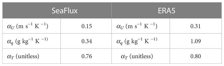
Moreover, this paper also makes use of the COARE3.5 bulk algorithm to obtain LHF from SST, U10m, 2 m relative humidity (RH2m) and T2m by means of the MOST (Fairall et al., 1996; Weller and Anderson, 1996; Fairall et al., 2003; Edson et al., 2013). COARE3.5 also needs information about the surface radiation balance, surface pressure, reference heights for the large-scale observations, latitude and height of the boundary layer to compute turbulent fluxes. For simplicity, all these parameters are set to the constant reference values presented in Table 1. No rain rate or wave-related corrections are considered and fluxes are computed from skin temperatures, with the exception of WRF data where bulk SST is considered. Therefore, the cool skin correction to the SST is not applied to SeaFlux and ERA5 and is considered in WRF.
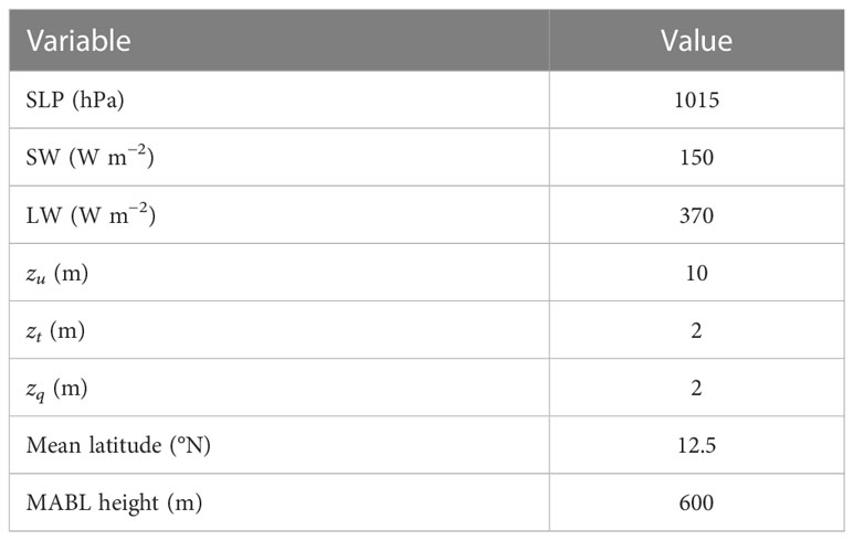
Table 1 COARE3.5 input parameters for SeaFlux and ERA5: Sea-level pressure (SLP), downward shortwave radiation (SW), downward longwave radiation (LW), wind sensor height (zu), bulk temperature sensor height (zt), humidity sensor height (zq), mean latitude of the EUREC4A-OA region and MABL height.
As stated in the Introduction, the relation between atmospheric and near-surface oceanic variables is quite different depending on the spatial scale considered, with the atmosphere generally forcing the ocean at the large scale and the ocean forcing the atmosphere at the mesoscale and below. In order to separate the large from the small-scale patterns, U10m, q2m, T2m and SST are filtered with an isotropic Gaussian filter as described in the Appendix. Hence, a given variable ψ is decomposed as
with being the filtered large-scale component and ψ′ the residual field, which contains small-scale information. The standard deviation of the Gaussian filter σ represents the threshold imposed to separate the small and the large-scale during the filtering (see the Appendix). Unless otherwise stated σ = 150 km, which roughly corresponds to the oceanic mesoscale; it also separates the larger scales at which the atmospheric winds directly impact ocean mixing and SST from the smaller scales at which the upper ocean thermal properties drive an atmospheric response (Seo, 2017; Gentemann et al., 2020).
The residual fields are used to study the strength of the air-ocean coupling. We indeed compute, through a linear regression, the coupling coefficients between SST’ and other variables such as U’10m, q’2m and T’2m. The resulting coupling coefficients are denoted as αU, αq and αT respectively and their statistical significance is assessed using a two-sided t test. These coupling coefficients are computed taking into account the residual fields at all (daily) time steps in a subset of the grid points in the EUREC4A-OA region. A sub-sampling has been introduced in order to consider spatially uncorrelated data, as detailed in the Appendix. A generic coupling coefficient is written as
The coupling coefficients are the core of the downscaling linear algorithm proposed in this study since they enclose all air-sea interaction processes. Given a certain SeaFlux/ERA5 variable (ψ) we build a new data set of the same variable including fine-scale SST features (ψHR) as
where ΔSST stands for the SST correction and represents the deviation of the high-resolution SST field with respect to the coarse SeaFlux/ERA5 SSTs. In order to ensure that the domain-averaged SST correction is zero and that the area-weighted means of the variables in the EUREC4A-OA region are conserved, ΔSST takes the following expression
Angle brackets denote the spatial average over the EUREC4A-OA region (Ω), namely
Hence, to refine an existing LHF data set we first remap the original SeaFlux/ERA5 U10m, q2m, T2m and SST to the MUR-JPL grid using the closest neighbor technique with Climate Data Operator (CDO) as described in Schulzweida et al. (2019). This is to avoid interpolated values which could potentially affect the results. Then, from these remapped data we compute LHF by means of COARE3.5 (LHFLR). Finally, we apply eq. 4 to the remapped SeaFlux/ERA5 variables and introduce them as an input in the COARE3.5 function. This operation provides the refined LHF data set (LHFHR).
To validate the downscaling procedure explained above and infer confidence in our results, numerical simulations using the WRF model have been used. Each simulation of a ten member ensemble is run from the 1st of December 2019 to the end of February 2020, forced at the lateral boundaries by ERA5 hourly data. At the lower boundary, the MUR-JPL SST product interpolated on the WRF numerical grid is used (in the following referred to as SSTWRF). The month of December 2019 is used as a spin-up and is not considered in the following analyses. The validation consists in creating lower resolution data starting from WRF outputs on the original model grid (at 3 km of resolution), that are then refined through the downscaling procedure described above. The obtained LHFHR field can be then compared with the original LHFWRF computed using the COARE3.5 formulation directly from WRF variables at 3 km grid spacing. To do so, we have produced lower resolution data, named SeaFlux-like data, by filtering WRF fields U10m, q2m, T2m and SST with a Gaussian filter considering σ = 24km. Such filtered fields are found to have spectral properties that are similar to the original SeaFlux data (not shown). These SeaFlux-like variables correspond to ψ variables in eq. 2, that we thus handle as if they were the original SeaFlux variables: we first compute the associated coupling coefficient and then we apply eq. 4. In the latter step, ΔSST is defined considering SSTHR ≡ SSTWRF.
Figure 1 shows the SeaFlux 2008-2018 DJF climatology in the EUREC4A-OA region. Like in most tropical regions, the atmospheric circulation is governed by the trade winds blowing from the open ocean towards South America. Their intensity decreases as they approach the coast (Figure 1B). SST and q2m present the same southwestern-northeastern gradient, both showing larger values towards the coast (Figure 1A). An exception to the SST general pattern is the presence of a cold patch close to the South American coast (Figure 1A) which likely corresponds to a coastal upwelling system (Acquistapace et al., 2022).
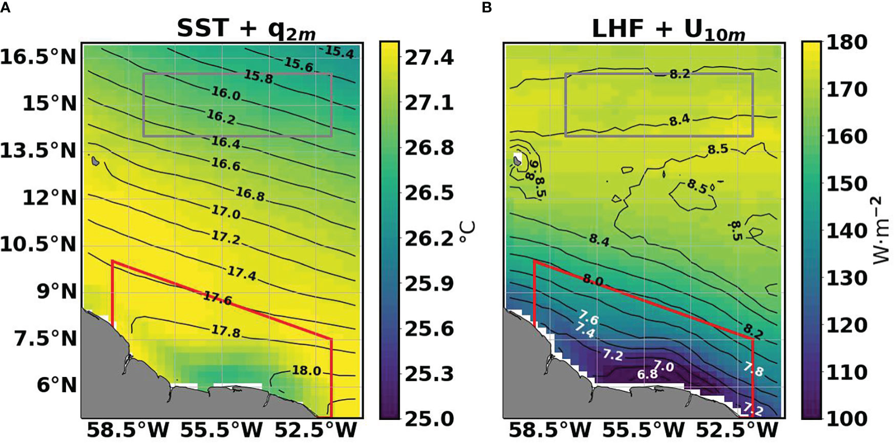
Figure 1 EUREC4A-OA region (5°-17°N, 60°-51°W) DJF climatology for SeaFlux. The shading in (A) represents the climatological SST and the contours stand for near-surface specific humidity (in g kg-1). In (B) the shading represents air-sea latent heat flux and the contours illustrate the mean values of near-surface wind speed (in m s-1, white color is used close to the coast to facilitate visualization). In both maps the gray box delimits the OOR (14°-16°N, 58°-52°W) and the red box represents the ECR. Daily values between 2008 to 2018 are considered to compute the climatologies.
The SST increase towards the coast is a consequence of a western boundary current (the North Brazil Current, NBC) and the anticyclonic eddies (the NBC rings) that this current regularly sheds, which advect northward tropical warm water towards the Caribbean Sea (Johns et al., 1990; Richardson et al., 1994). The saturation water vapor specific humidity is smaller in the open ocean, in line with what expected by the Clausius-Clapeyron relation for evaporation over colder waters. The q2m and SST fields, together with the decreased wind speeds near the coast (Figure 1B), imply lower values of LHF in shelf waters than in the open ocean (Figure 1B). Based on these spatial differences, the EUREC4A-OA domain is traditionally divided into two sub-regions (Stevens et al., 2021): the NBC eddy corridor region (ECR) and the open ocean region (OOR). They are displayed as the red and grey areas in Figure 1 respectively.
To deepen our understanding in the dynamic and thermodynamic differences between these two regions, Figure 2 represents the histograms of the oceanic and near-surface atmospheric variables analyzed in this paper for the whole EUREC4A-OA, for the ECR and for the OOR. Figures 2A, B represent the SST distribution and show that the ECR is characterized on average by warmer SSTs than the OOR.
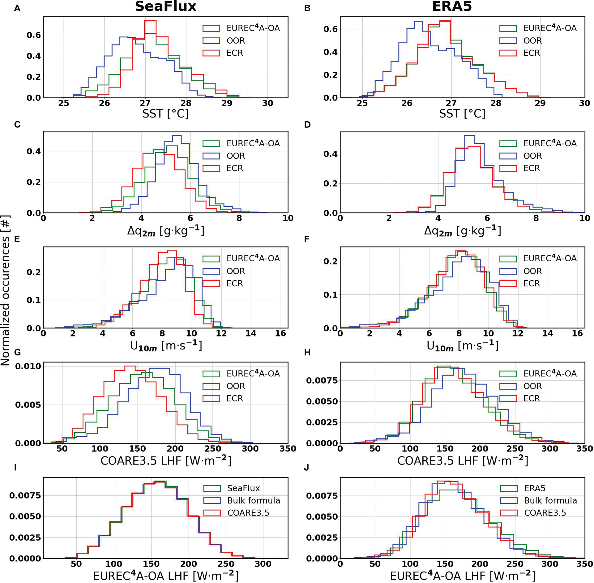
Figure 2 Histograms of the different variables analyzed in this paper for SeaFlux (left column) and ERA5 (right column). (A, B) represent the SST; (C, D) depict the 2 m specific humidity deficit defined as the difference between the saturation specific humidity and q2m; (E, F) illustrate the U10m distribution and (G, H) display LHF computed using COARE3.5. In all the plots hitherto mentioned the green curve is obtained considering the whole EUREC4A-OA box (5°-17° N, 60°-51°W), and the blue and red histograms are calculated over the OOR and ECR regions respectively as defined in the main text and as shown in Figure 1. (I, J) represent the LHF given directly in the data sets (green), computed using eq. 1 (blue) and using COARE3.5 (red). All the histograms are constructed using daily averages of SeaFlux and ERA5 data in the 2008-2018 DJF season.
Figures 2C, D represent the specific humidity deficit (Δq) distribution, defined as the difference between q* and q2m. They show that Δq is smaller in the ECR, especially in Figure 2C corresponding to SeaFlux. In turn, the whole EUREC4A-OA region and the OOR present similar specific humidity deficit distributions. Accordingly, the U10m distribution represented in Figures 2E, F shows lower values in the ECR and a wider probability density function (PDF) for the OOR with values ranging from 2 m s-1 to 12 m s-1 in both data sets.
In agreement with eq. 1, decreased Δqs and U10ms lead to lower LHFs in the ECR region. This is shown in Figures 2G, H. Finally, we also check that different LHF estimates provided by three possible ways to compute LHF (eq. 1, COARE3.5 and the LHF provided directly by SeaFlux and ERA5) do not present substantial differences for both, SeaFlux and ERA5 (Figures 2I, J). No difference is observed in SeaFlux between the three estimates (Figure 2I) since this satellite-based product uses COARE3.0 to derive LHF (Clayson et al., 2014). This algorithm does not differ from COARE3.5 in the turbulent-flux calculation part. For ERA5, we observe slight differences between COARE3.5 and the LHF provided by ERA5 and eq. 1 (Figure 2J). These differences are expected as ERA5 does not use COARE3.5 to compute THFs. However, the deviations are less than 10 W m−2, much smaller than the characteristic LHF differences discussed in this manuscript. Therefore, all the fluxes of this article are hereon calculated with COARE3.5 only. The bulk formula in eq. 1 is also used for theoretical considerations.
Given the spatial heterogeneity of the EUREC4A-OA region shown in Figures 1, 2, point-wise regressions are performed between SST and q2m and U10m. They are shown in Figure 3. White contours in Figures 3A, B show the regression coefficient between the smoothed SST and q2m fields for SeaFlux and ERA5 respectively. In both cases, the large-scale near surface specific humidity increases with SST in all the locations of the EUREC4A-OA region in agreement with the fact that warmer air needs more water vapor to reach saturation. The estimated coupling coefficients range between 0.84 g kg-1 K-1 and 1.27 g kg-1 K-1, slightly less than the Clausius-Clapeyron scaling αq* ~ 1.3 g kg-1 K-1. Such a scaling is obtained with a linearization of the Clausius-Clapeyron expression of Buck (1981) (as used in COARE3.5) around the reference SST value of 300 K, representative of the region (see the Appendix for the full derivation). Physically, this corresponds to the fact that at large scales there is enough evaporation so that the near-surface specific humidity is close to saturation.
Conversely, the coupling coefficients of the SeaFlux SST-q2m residual fields indicate that, at the small-scale, the Clausius-Clapeyron scaling is not respected (Figures 3A, B). The SeaFlux residual coupling coefficients range from -0.4 to -0.1 g kg-1 K-1 and the ERA5 ones lie between 0.1 and 0.4 g kg-1 K-1, in both cases significantly smaller than the 1.3 g kg-1 K-1 reference value. This fact is interpreted in terms of a more complex atmospheric response to the small-scale oceanic forcing. In fact, warmer SSTs are associated with a more unstable MABL. This configuration enhances vertical mixing within the MABL, entrainment at the MABL top and a subsequent MABL thickening. Hence, at least two mechanisms contribute to the decrease of αq: (1) the thickening of the MABL that dilutes the air water content, and (2) the mixing at the top of the MABL which entrains dryer air from the free atmosphere (Neggers et al., 2006; Acquistapace et al., 2022; Albright et al., 2022).
Note that the SeaFlux q2m coupling coefficients are negative over most of the EUREC4A-OA domain (Figure 3A) whereas the ERA5 ones remain slightly positive (Figure 3B). This fact might suggest that the MABL dynamical mechanisms which reduce the surface specific humidity are weaker in ERA5 than in SeaFlux. It is likely that the numerical parametrizations used in the ERA5 model are not capable to correctly reproduce the MABL dynamics. In particular, the schemes that parameterize the surface fluxes and the MABL turbulence might play a major role (Perlin et al., 2014). Elucidating the specific causes of this difference requires further research which is not presented here as it goes beyond the scope of this study. What matters for our purposes is that the coupling coefficients of the specific humidity from both SeaFlux and ERA5 residuals are different from the Clausius-Clapeyron scaling, consistent with the fact that air moving over small SST structures does not have the time to reach an equilibrium condition with the sea underneath.
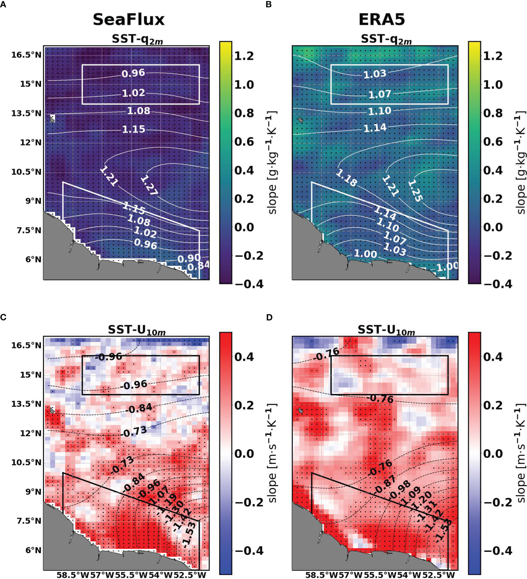
Figure 3 Spatial distribution of the and SST-q2m and SST-U10m linear regression slopes for SeaFlux (left column panels) and ERA5 (right column panels). (A, B) represent the SST-q2m linear regression slopes for the smoothed (contours, in g kg−1 K −1 and in white to facilitate visualization) and residual fields (shading). (C, D) represent the SST-U10m linear regression slopes for the smoothed (contours, in m s−1 K −1) and residual fields (shading). In all the cases, the hatching marks the slopes from the residual fields which are statistically significant at a 99% confidence interval after a two-sided t-test. All the panels are obtained considering daily data during the 2008-2018 DJF season. The σ value introduced in the Gaussian filter equals 150 km. In all the maps the OOR and the ECR are delimited by the northern and coastal boxes respectively.
The large-scale U10m and SST linear regression slopes are shown in black contours in Figures 3C, D for SeaFlux and ERA5 respectively. They are negative over almost the whole EUREC4A-OA region. They reach their minimum over the NBC retroflection, perhaps as a result of the increase in SST and the weakening of surface winds as we approach the equator. The negative coupling coefficients are often interpreted as a consequence of the ocean responding passively to the atmospheric forcing. Higher near-surface wind speeds are responsible for increased LHF and enhanced mixing in the upper ocean. These two factors result in a decrease of SST.
Instead, positive coupling coefficients for the residual U10m and SST fields dominate over the EUREC4A-OA region, especially in the ECR (shading in Figures 3C, D). In the attempt to explain how small-scale SST features affect surface winds, two mechanisms have been previously identified: the pressure adjustment (PA) mechanism (Lindzen and Nigam, 1987) and the downward momentum mixing (DMM) (Hayes et al., 1989; Wallace et al., 1989). In the PA mechanism the thermal expansion of air over warm SST patches generates pressure anomalies that drive a secondary circulation characterized by surface wind convergence at the center of the warm anomaly. Similarly, surface wind divergence occurs over cold anomalies. This implies weak surface wind velocities both at SST maxima and minima, and therefore no correlation SST-U10m. In turn, the DMM mechanism expresses that, when an air parcel crosses a SST front going from cold to warm water, its buoyancy increases and reduces the static stability of the air column. This enhances a downward flux of horizontal momentum from the top of the MABL to the surface, triggering the entrainment of higher values of wind speed into the MABL thereby increasing surface wind speed on the warm side of the front, this results in a positive SST-U10m correlation. The positive and statistically significant αUs shown in Figures 3C, D, especially in the ECR, suggest the DMM mechanism is here at play and it dominates the small-scale SST-U10m interactions. A more detailed discussion on the two mechanisms, involving different metrics computed in the EUREC4A-OA region, can be found in the Appendix.
So far, the spatial distribution of the coupling coefficients has been assessed for a fixed value of σ = 150 km. To obtain a deeper insight into the dependence of the SST-MABL coupling on the spatial scale, we consider a wider range of σ values. In particular, we compute αU and αq for σ ranging from 100 km to 1000 km (Figure 4). The coefficients computed for σs smaller than 100 km (the effective resolution of the data sets according to the autocorrelation analysis of the Appendix) are not presented in Figure 4 as they do not contain anything but random noise. The sub-sampling spacing to compute the coupling coefficients presented in Figure 4 is taken as 150 km regardless of the σ value. The reasons for this choice are explained in the Appendix.
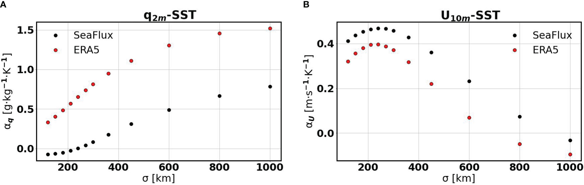
Figure 4 DJF coupling coefficients computed from SeaFlux (black dots) and ERA5 (red dots) residual fields as a function of σ using a constant autocorrelation length of 150 km for spatial sub-sampling. (A) represents αq and (B) stands for αU. The time period considered is the DJF season 2008-2018 in all the cases and the slopes are computed considering the whole EUREC4A-OA region. No error bars are included as the standard errors associated to the linear regression slopes are within the size of the markers.
Figure 4A shows that αq monotonically grows with increasing σ for the two data sets. In ERA5, it tends to the Clausius-Clapeyron scaling value of 1.3 g kg-1 K-1. Apart from the difference in value (the SeaFlux coupling coefficient is always 0.5 g kg-1 K-1 - 0.7 g kg-1 K-1 smaller than ERA5), all the data sets provide low values of the coupling coefficients for small values of σ. This suggests that, at small-scales, specific humidity does not adjust to SST anomalies with values close to saturation as relative humidity changes and advection probably mask the direct relationship expected from Clausius-Clapeyron. Instead, the dynamical MABL response to the small-scale SST structures reduces the specific humidity dependence on SST, because of the modulation of the MABL height and its mixing. In turn, the SST-U10m coupling coefficients for SeaFlux and ERA5 are generally positive, as expected from the DMM mechanism (Figure 4B). In addition, as σ increases, the coupling coefficients of SeaFlux and ERA5 decrease as larger-scale features are retained in the residual fields, in agreement with the change of atmosphere-ocean coupling between large and small scales discussed in section 1.
Note that both SeaFlux SST-q2m and SST-U10m coupling coefficients present a tendency change at around σ = 200 km. As we approach σ = 200 km from larger σ values we observe a change in sign from positive to negative in αq (Figure 4A) and the maximum value of the αU-σ scatter plot (Figure 4B). Such behaviors are consistent with all the discussion of the preceding paragraphs regarding the small-scale SST-near-surface atmosphere linkages as 200 km is roughly the limit between the ocean mesoscale and the large-scale. This fact also supports our choice of 150 km as the separation scale to define the residual fields.
The estimated coupling coefficients will be used in the following to downscale the impact of the small-scale SST on the LHF. Even though they have been proven to be sensitive to the spatial scale considered and the specific location within the EUREC4A-OA region, for simplicity, only the coupling coefficients in Figure 4 for σ = 150 km have been used in the rest of the work and are shown in Table 2. However, for the sake of completeness, the coupling coefficients in the ECR and OOR as defined in Figure 1 for σ = 150 km are also provided in Tables 3, 4 respectively. All the calculations in next section are also performed with these coupling coefficients as well in order to give an estimate of the variability of the results as a function of the spread in the coupling coefficients.
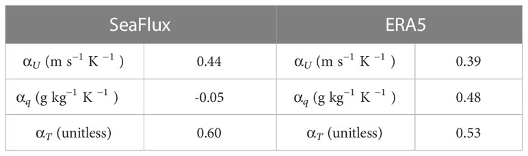
Table 2 Coupling coefficients for U10m (aU), q2m (aq), and T2m (aT) used in the downscaling algorithm for SeaFlux and ERA5.
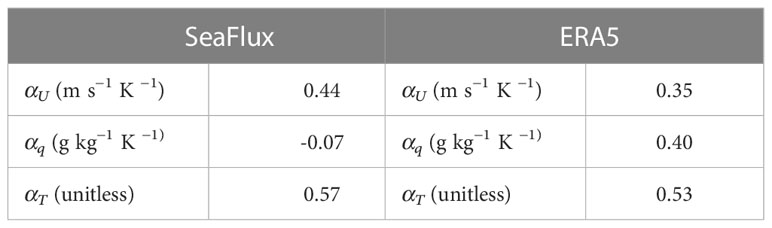
Table 3 As in Table 2 but for the ECR.
Figures 5A, B represent the averaged 2008-2018 DJF difference between LHFHR and LHFLR for SeaFlux and ERA5 respectively. Recall that for SeaFlux and ERA5, LHFHR represents the COARE3.5 latent heat flux output computed from the U10m, q2m, T2m and SST given by eq. 4 and that LHFLR is the COARE3.5 latent heat flux output obtained from the remapped U10m, q2m, T2m and SST. These two LHFs show differences up to 10 W m-2 in coastal areas of the ECR. Weaker LHF values prevail by moving towards the OOR. The quantities in brackets over Figures 5A, B represent the area-weighted means of the LHF differences. They are close to zero for both datasets. This means that, away from the locations where ΔSST is large (i.e. the ECR), the O (ΔSST2) effects in the LHF controlling variables (U10m, q2m, SST and T2m) do not produce large LHF variations so that LHF evolves almost linearly with ΔSST. Accordingly, the spatial pattern of the LHF differences coincides with the size of the ΔSSTs shown in Figures 5C, D for SeaFlux and ERA5 respectively.
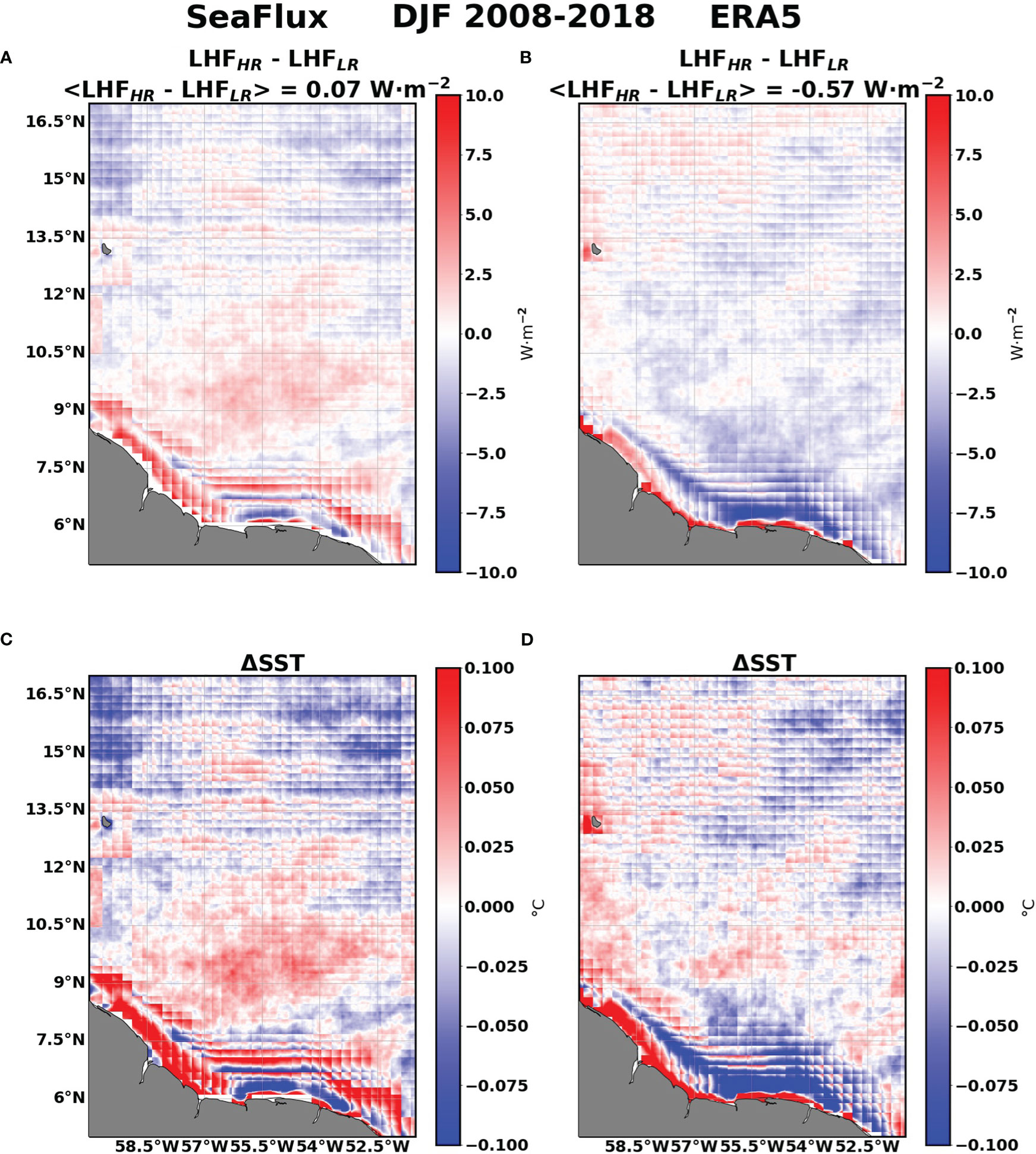
Figure 5 2008-2018 DJF mean of (A, B) difference between the reconstructed LHF from the downscaled near-surface variables and SST (LHFHR) and the LHF obtained from the raw SeaFlux/ERA5 variables (LHFLR). (C, D) represent the 2008-2018 DJF mean of the SST correction (ΔSST) for SeaFlux/ERA5. Angle brackets in the titles of the figures represent the area-weighted mean values of the variables represented on the corresponding subplot.
The differences of 10 W m-2 shown in Figures 5A, B only represent around 5 – 7% of the mean LHF in the EUREC4A-OA region (shading in Figure 1B). These deviations are reduced when averaged over the 10 DJF seasons because the characteristic lifetime of the fine-scale ocean features whose effects on LHF we aim to analyze ranges from days to months. As a consequence, it is interesting to look at daily snapshots of the LHF bias and ΔSST in order to study the response of LHF to these fine-scale SST structures. Let us then consider Figure 6 which depicts the same fields as Figure 5 but for the 1st of December 2008. Biases up to 60 W m-2 in absolute value are observed, (Figures 6A, B) especially in the ECR which are equivalent to 30% to 40% of the climatological LHF (shading Figure 1B), responding to ΔSSTs not exceeding 1°C in absolute value (Figures 6C, D). Again, the spatial pattern of the LHF differences resembles to that of the SST correction suggesting a linear relationship between the two quantities. We come back to this point in the next paragraphs.
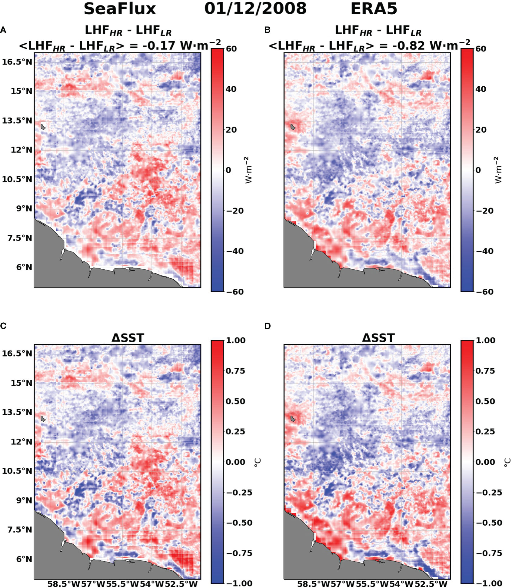
Figure 6 01/12/2008 values of (A, B) difference between the reconstructed LHF from the downscaled near-surface variables and SST (LHFHR) and the LHF obtained from the raw SeaFlux/ERA5 variables (LHFLR). (C, D) represent the 01/12/2008 values of the SST correction (ΔSST) for SeaFlux/ERA5. Angle brackets in the titles of the figures represent the area-weighted mean values of the variables represented in the corresponding subplot.
So far, the downscaling has been applied using the coupling coefficients computed accounting for the whole EUREC4A-OA region. However, the coupling coefficients present strong spatial variations within the EUREC4A-OA region (Figure 3) which have an impact in the resulting downscaled fluxes. To provide an estimate on how large this effect is, we downscale the LHF using the coefficients in Tables 3, 4 corresponding to the ECR and OOR respectively. Strong deviations of the order of 40% to 50% are observed in both cases for particular days of the 2008-2018 DJF period, evincing the importance of maintaining the distinction between sub-regions in the downscaling.
Given the large LHF variations with SST, we try here to separate the different mechanisms by which the fine-scale SST structures may influence LHF. This concept is hereafter referred to as LHF sensitivity to SST. We group these mechanisms into two main categories: the thermodynamic contribution and the dynamic contribution. The thermodynamic contribution includes only the increased LHF at larger SST due to the Clausius-Clapeyron dependence of saturation water vapor pressure to SST, while the surface relative humidity and the air-sea temperature difference are considered to be fixed. The dynamic contribution relates to the MABL response to increased SST, which reduces air-column stability, increases the vertical mixing in the lower troposphere, and favors entrainment at the top of the MABL, resulting in increased surface winds and specific humidity deficit, both of which enhance the LHF from the ocean into the atmosphere.
In order to theoretically quantify the importance of each contribution, let us consider the bulk formula for LHF (eq. 1). We choose the most frequent values of the corresponding histograms in Figure 2 as representative quantities for the EUREC4A-OA region: U10m = 9m s-1, q* = 21.7g kg-1 (saturation specific humidity at 27°C) and q2m = 15.5g kg-1, Ce = 1.6·10-3. This leads to LHF ≃ 160 W m-2 using eq. 1. Consider now that SST is increased by 1°C and compute first the thermodynamic change of LHF: the only term that changes is (q* − q2m) which, assuming a constant relative humidity, increases by ∂q*/∂SST(1−q2m/q*)≃0.31 g kg-1 K-1. Considering that (q* − q2m) is about 5.5 g kg-1, this results in an increase in LHF of about 5% (=0.31/5.5), per the 1°C increase in SST.
Using the SeaFlux coupling coefficients shown in Table 2, we compute the effect of the dynamic response on LHF: U10m increases by 0.44 m s-1 K-1, which means a relative increase of 4.9% (=0.44/9), (q* − q2m) increases by about 1.3 g kg-1 (we consider here q2m vs SST slope equal to 0, 1.3 g kg-1 is the increase in q* when SST changes from 26°C to 27°C) - relative increase of (q* − q2m) is about 24% per °C (=1.3/5.5). In total, the sensitivity of LHF to SST through the dynamic response is about 28% per °C, a factor of about 4-5 larger than the thermodynamic response. Putting all together, the sensitivity of LHF to SST is about 33% per °C.
We perform the same calculation with the SeaFlux coupling coefficients shown in Tables 3, 4 in order to have an estimate of the spatial variability of the LHF sensitivity to SST within the EUREC4A-OA region. According to Figure 2, the ECR has a typical SST of 27.1°C, Δq is about 4.1 g kg-1 with q*~ 22 g kg-1 and q2m~ 18 g kg-1. Moreover, U10m = 8m s-1 and αU ~ 0.44 m s-1 K-1. These values produce a thermodynamic and dynamic contributions of around 6% and 37% of LHF change per °C of SST respectively. These two contributions together represent a change of 43% of LHF change per °C. Conversely, for the OOR we have SST~ of 26.8°C, Δq is about 5.8 g kg-1 with q*~ 21.5 g kg-1 and q2m~ 16 g kg-1. Moreover, U10m = 9m s-1 and αU ~ 0.15 m s-1 K-1. These values result in a thermodynamic contribution of around 6% and a dynamic contribution of 24% producing a total sensitivity of LHF to SST of the order of 30%. Therefore, LHF is not impacted by SST variations in the same way in the entire EUREC4A-OA region. The difference comes mainly from the fact that the MABL response to fine-scale SST structures is weaker in the OOR than in the ECR.
We also test the results from the last two paragraphs using SeaFlux and ERA5 data. To compute the total LHF sensitivity to SST we perform a linear regression between the relative change in LHF (100· (LHFHR − LHFLR)/LHFLR) and ΔSST. The results for SeaFlux and ERA5 are shown in Figure 7A in blue and red respectively. The estimated LHF change per °C for SeaFlux (33.8% per °C) agrees with the theoretical value mentioned above whereas the ERA5 LHF sensitivity to SST is weaker (26.6% per °C). The shading in Figure 7A indicates the range of different LHF variations obtained between the OOR (lower limit) and the ECR (upper limit) for SeaFlux (ERA5 results are not included as they do not modify the analysis and conclusions). It aims to provide an estimate of the uncertainty in the linear regressions associated to the geographical heterogeneity of the MABL response to fine-scale SST structures. For small values of ΔSST, the LHF variations are similar within the EUREC4A-OA region. However, for |ΔSST| larger than 0.5°C we obtain LHF variations ranging from ±20% - ±40% in the OOR and ECR respectively. Figure 7A also allows us to identify that for SST corrections with absolute values lower than 0.5°C, the LHF response is almost linear despite COARE3.5 being a non-linear algorithm. Beyond the ± 0.5°C threshold, LHF changes become stable around ±20% - ±30%.
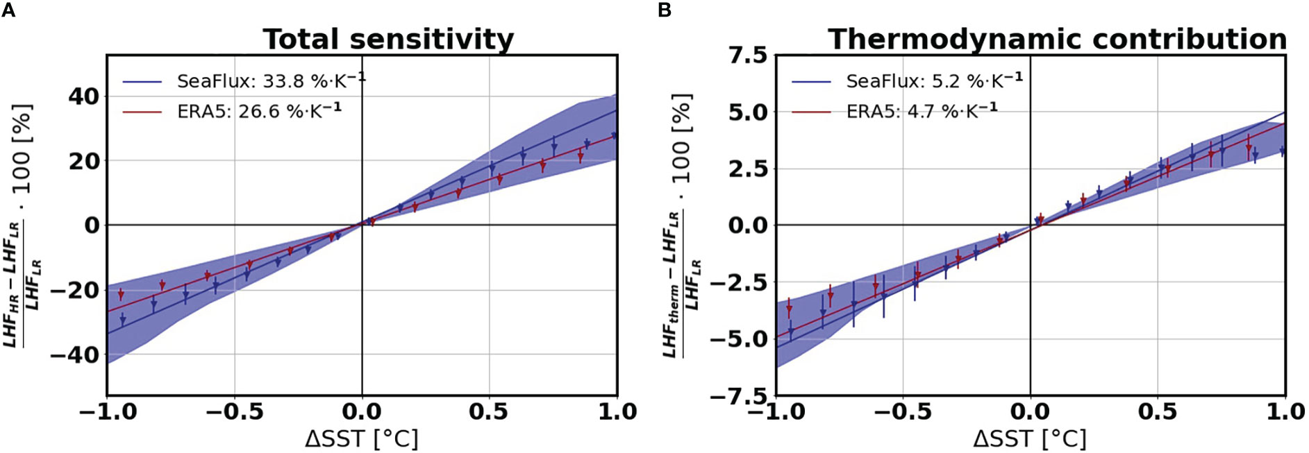
Figure 7 Binned scatter plot and linear regression between ΔSST and the LHF relative error when (A) all the input COARE3.5 variables are downscaled (LHFHR) and (B) when ΔSST is only added to T2m and SST. SeaFlux results are represented in dark blue and the ERA5 output in dark red. Data are taken for the 2008-2018 DJF season and are binned in 0.1°C-wide ΔSST intervals. The mean value of each bin is represented with dots and the error bars illustrate the standard deviation of each bin. The slopes of the regression lines are provided in the upper left side of each panel. In both panels, the shading indicates the lower and upper limits of the LHF sensitivity to SST obtained when the downscaling (in A) and correction (in B) of the COARE3.5 input variables is performed only over the OOR and ECR respectively for SeaFlux. The ERA5 ECR and OOR LHF sensitivity to SST results are not included to facilitate visualization.
In order to isolate the thermodynamic contribution in the LHF sensitivity, a new LHF data set (LHFtherm) is produced with COARE3.5. In this case, only SST and T2m are modified by adding the SST correction (the coupling coefficients are not involved here). This is to keep the vertical MABL temperature gradient, q2m and U10m as constant values. Again, we perform a linear regression between the relative change in LHF and ΔSST and study the value of the slopes (Figure 7B). In agreement with the theoretical result, the thermodynamic contribution accounts for the 5.2% per °C of SST of LHF change in SeaFlux. Accordingly, ERA5 provides a slightly weaker sensitivity of 4.7% per °C of SST. In Figure 7B we also appreciate the boundaries of the linear regime and the importance of treating separately the different sub-regions of the EUREC4A-OA domain to accurately determine the LHF variations associated to fine-scale SST structures, especially for large values of |ΔSST|.
We validate our approach by means of the original high-resolution LHF obtained from the original simulated WRF variables using the COARE3.5 algorithm (Figure 8A). This LHF dataset, which we denote as LHFWRF, is physically consistent with the fully compressible Euler equations and, thus, can be considered a reliable source of high-resolution information.
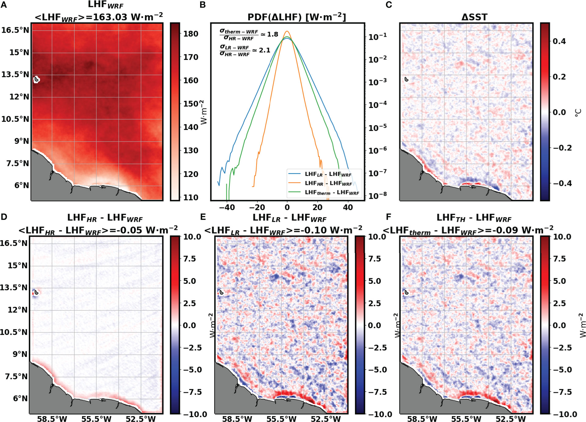
Figure 8 Validation with WRF data. In the figure, LHFs are all computed by means of the COARE3.5; LHFWRF is the LHF computed from WRF atmospheric and oceanic outputs, LHFLR represents the LHF computed from upscaled WRF data (using a Gaussian filter with σ = 24 km) and LHFHR stands for the LHF data set computed after having applied the downscaling technique to q2m, U10m, T2m and SST. LHFtherm represents the only thermodynamic contribution to LHF, obtained from the correction of T2m and SST with ΔSST. (A) Map of mean LHFWRF. (B) PDF of LHFLR- LHFWRF (blue curve), LHFHR - LHFWRF (orange curve) and LHFtherm - LHFWRF (green curve). (C) Map of mean SST correction (ΔSST). (D-F) Maps of the mean difference between LHFHR, LHFLR,LHFtherm (respectively) and the reference LHFWRF. All the means are computed over JF and the 10 members of the WRF model.
To test the robustness of the downscaling approach, we look at the difference between LHFWRF and LHFLR,HR,therm. To estimate the downscaled LHFs we use the coupling coefficients computed from LHFLR that do not differ significantly from Seaflux (not shown). Results in Figure 8 show that LHFHR obtained from the downscaling best represents LHFWRF both in terms of spatial patterns (Figure 8D) and in terms of spatial-temporal statistics (Figure 8B). Figure 8B displays the PDFs of differences of LHFLR (blue curve), LHFtherm (green curve) and LHFHR (orange curve) with LHFWRF; the latter is the narrowest PDF among the three showing that the downscaling approach we have implemented to isolate the small-scale ocean influence on the atmosphere reduces (approximately by a factor 2) the biases between LHF datasets.
Concerning the spatial structure of LHFs, Figures 8D–F display the differences LHFHR -LHFWRF, LHFLR -LHFWRF and LHFtherm -LHFWRF respectively. They show that LHFHR accurately represents the reference LHF both in magnitude and in the spatial distribution of the bias. The spatial patterns in Figures 8C, E, which are similar to each other, are determined by ΔSST (Figure 8C) confirming the linear relationship of the downscaling as in the case of Figure 7A. However, the magnitude of the correction provided for the downscaling applied to the WRF simulated fields is smaller than in the case of SeaFlux. This is due to the fact that the range of ΔSST correction (Figure 8C) is much smaller for WRF than for SeaFlux in Figure 7A.
It is also interesting to note that the correction ΔSST in Figure 8C differs from Figures 5C, D also in terms of spatial patterns. The former presents only small-scales correction, while in the latter large-scales structures emerge. This might be due to the contribution to the correction in Figures 5C, D from two different products (SeaFlux and MUR-JPL) while Figure 8C is obtained only with MUR-JPL. The inconsistencies and biases between these two different data sets do not allow us to directly compare the spatial SST correction patterns and might also explain the noisy pattern shown in Figure 5.
This study assesses how fine-scale SST structures influence LHF in the north-west tropical Atlantic Ocean in winter. In order to do that, it is first necessary to understand how the near-surface atmospheric variables are related to SST. We find that this relationship depends on the spatial scale of interest. The analyses of the SeaFlux satellite-based product show that for scales of the order of or smaller than 150 km, q2m tends to decrease when SST increases whereas U10m increases by virtue of the DMM mechanism. The change rates are -0.05 g kg-1 K-1 and 0.44 m s-1 K-1 respectively as shown in Table 2. However, these results are highly dependent on the data set analyzed. In ERA5 (Table 2), the q2m-SST coupling coefficient has the opposite sign to that of SeaFlux (0.48 g kg-1 K-1) and αU is 0.44 m s-1 K-1.
Our work also highlights the impact, in these coupling coefficients, of the environmental conditions (such as the strength of the prevailing winds) and dynamics which affect their magnitude. The area we studied is characterized by two dynamically different domains: a relatively quiet and homogeneous open ocean and the North Brazil Current ring (eddy) corridor encompassing the South American continental shelf and slope. In the latter, the small-scale U10m variations with SST are stronger than in the open-ocean domain (0.44 m s-1 K-1 versus 0.15 m s-1 K-1 as shown in Tables 3, 4). Conversely, the changes in q2m are higher in the open ocean than in the eddy corridor, possibly as a consequence of the enhanced fine-scale activity in the latter masking the Clausius-Clayperon relationship (-0.07 g kg-1 K-1 in the ECR versus 0.34 g kg-1 K-1 in the OOR as depicted in Tables 3, 4). This suggests that the environmental conditions such as the presence of an inversion layer at the top of the MABL and the speed of the prevailing winds as well as a different ocean dynamical environment likely affect the sensitivity of the boundary layer properties to the SST. For those reasons, the coupling coefficients and the amplitude of the LHF anomaly obtained from the downscaling procedure are expected to have different magnitudes in different geographical areas and seasons. In particular, it would be interesting to apply the methodology of this study to regions with stronger SST gradients and important mesoscale activity such as the Gulf Stream, the Kuroshio Extension or the Southern Ocean. Apart from ameliorating our understanding of the SST-MABL processes in these regions it could potentially provide a powerful tool to enhance our knowledge on low cloud formation and on air-sea fluxes, with numerous applications in weather forecasting and climate projections.
The interplay described here is therefore only part of a complex series of interactions involving the coupled ocean–atmosphere system which includes two-way interactions between the MABL and the upper ocean. The SST-induced wind disturbances cause perturbations in surface heat fluxes and upper-ocean mixing that are likely to erode SST anomalies that will feed back into the original wind stress perturbations. Moreover, the upwelling associated with SST-induced wind stress curl perturbations will feed back on the ocean, likely altering the SST Small et al. (2008). These two-way feedbacks are intriguing aspects of the coupled system that can significantly enhance our understanding of ocean–atmosphere interactions.
The fine-scale coupling coefficients we derived are at the core of the downscaling algorithm we developed in this work to assess the small-scale SST influence on LHF. When the influence of the ocean small scales is taken into account, the LHF magnitude increases on average of 33% per °C. Further analyses allowed us to distinguish two different mechanisms at play: the thermodynamic and dynamic contributions. The former includes only the increase of LHF with SST associated to the Clausius-Clapeyron dependence of saturation water vapor pressure on SST. The latter is related to the modification of the vertical stratification of the MABL as a consequence of SST anomalies. From SeaFlux we estimate that they represent a LHF increase of 5% and 28% per °C respectively, in agreement with what the LHF bulk formula and previous research predict. Using Surface Wave Instrument Float with Tracking (SWIFT) and Wave Glider observations measured during the ATOMIC campaign as well as satellite data, Iyer et al. (2014) are able to detect differences up to of 30% in LHF across SST gradients (average SST difference of 0.7°C over a distance of 44 km). Our results show that the LHF amplitude is also affected by the geographical heterogeneity of the coupling coefficients. As a result, LHF in the eddy corridor shows the largest variations (around 43% per °C of SST). To provide substantiation to our results, we tested the downscaling approach against an ensemble of one-month long high-resolution regional atmospheric simulations forced at the lower boundary by a high-resolution SST product and at the open boundaries by ERA5. This test shows that the downscaling reduces by a factor of 2 the difference between the simulated and reconstructed LHF fields proving the soundness of the approach.
Our study, however, does not investigate all the processes involved in the near-surface atmospheric response to fine-scale SST structures. For instance, the downscaling technique assumes that all near-surface variables depend exclusively on SST and disregards the nonlinear cross-terms like the increase of air water vapor content due to wind advection. Furthermore, this work does not account for the surface current effect on LHFs estimate. This fact might result in possible inaccuracies, especially in regions characterized by intense mesoscale activity such as the North Brazil current eddy corridor, where surface currents velocity are high (they can exceed 1 m s-1) (Seo, 2017; Renault et al., 2019; Zhang et al., 2021). To test how this effect weights in in LHF, we use data from the two NOAA-funded Saildrones of the EUREC4A-OA/ATOMIC experiment (Stevens et al., 2021): SD1063 and SD1064. These wind-propelled uncrewed surface vehicles were equipped with different sensors collecting measurements at the air-sea interface (e.g., SST, sea-surface salinity, winds, air temperature…) at 1-minute temporal resolution thereby offering an unprecedented view of the upper ocean and the air-sea interface. They were also equipped with an Acoustic Doppler Current Profiler (ADCP) on the keel, allowing to monitor the upper ocean currents. SD1063 sampled parts of the eddy corridor while SD1064 navigated through the open-ocean sector of the EUREC4A-OA domain. Using these in-situ measurements, we find that the intense surface currents at the edge of mesoscale eddies induce a change of almost 5% to 15% in LHF (not shown). This suggests that other data sources are needed in order to further explore the effects of fine-scale SST structures on air-sea fluxes. The high temporal resolution of in-situ data from the EUREC4A-OA/ATOMIC campaigns (Quinn et al., 2021; Stevens et al., 2021) are likely to provide better estimates of the impacts of SST gradients on air-sea fluxes that go beyond the coarse (with respect to the ocean small-scale) spatial grid of available satellite observations.
The data sets analyzed for this study can be found in the following open-access repositories.
● SeaFlux, https://seaflux.org/seafluxdata/ATOMICcurrent/
● ERA5, https://cds.climate.copernicus.eu/cdsapp!/dataset/reanalysis-era5-single-levels?tab=form
● MUR-JPL, https://thredds.jpl.nasa.gov/thredds/ncss/grid/OceanTemperature/MUR-JPL-L4-GLOB-v4.1.nc/dataset.html
● WRF outputs, due to their large memory size, are available from the authors upon request.
● The additional data used in the Appendix are available from the Centre for Environmental Data Analysis (CEDA) archive: https://dap.ceda.ac.uk/neodc/esacci/sst/data/CDRv2/.
All the authors contributed to conception and design of the study. SS and PF organized the SeaFlux, ERA5 and MUR-JPL databases and performed the statistical analysis with them. In turn, AM, MB, FD, and CP organized the WRF model database and performed the statistical analysis with it. PF wrote the first draft of the manuscript and the sections which did not involve analysis with the WRF model. AM, MB, FD, and CP wrote sections of the manuscript related to the WRF data description and the downscaling algorithm validation. The separation technique between the thermodynamic and dynamic contributions of LHF sensitivity to SST was performed by AM, MB, and CP. All authors contributed to the article and approved the submitted version.
PF is funded by a PhD grant of the Doctoral School of Environmental Sciences in Île-de-France N°129. FD is funded by Piano Operativo Nazionale “Ricerca e Innovazione”, Italian Ministry of University and Research (2021-RTDAPON-150). MB is funded by the Joint Programming Initiative ClimateOceans (project EUREC4A-OA). AM has received support from the European Space Agency (ESA) as part of the GLAUCO Climate Change Initiative (CCI) fellowship (ESA ESRIN/Contract No. 4000133281/20/I/NB).
The authors acknowledge the contributions of Carol Anne Clayson and Jeremiah Brown from the Woods Hole Oceanographic Institution (WHOI) for providing the new, high-resolution, SeaFlux dataset. In addition, the authors would like to thank Dr. Dongxiao Zhang from NOAA for the fruitful discussions on the different bulk flux algorithm as well as on his work highlighting the effect of surface ocean currents on air-sea fluxes which serves as inspiration for further research. The authors thank the two reviewers who helped to clarify results presented. This work is a contribution to the EUREC4A-OA project, funded jointly through JPI Oceans and JPI Climate. Part of this work is an outcome of the project MIUR – Dipartimenti di Eccellenza 2018–2022.
The authors declare that the research was conducted in the absence of any commercial or financial relationships that could be construed as a potential conflict of interest.
All claims expressed in this article are solely those of the authors and do not necessarily represent those of their affiliated organizations, or those of the publisher, the editors and the reviewers. Any product that may be evaluated in this article, or claim that may be made by its manufacturer, is not guaranteed or endorsed by the publisher.
Acquistapace C., Meroni A. N., Labbri G., Lange D., Späth F., Abbas S., et al. (2022). Fast atmospheric response to a cold oceanic mesoscale patch in the north-western tropical Atlantic. J. Geophys. Res.: Atmospheres 127, e2022JD036799. doi: 10.1029/2022JD036799
Albright A. L., Bony S., Stevens B., Vogel R. (2022). Observed subcloud-layer moisture and heat budgets in the trades. J. Atmospheric Sci. 79, 2363–2385. doi: 10.1175/JAS-D-21-0337.1
Arfken G. B., Weber H. J. (2005). Mathematical methods for physicists. 6th ed. (Amsterdam: Elsevier Academic Press), 1182 pp.
Bishop S. P., Small R. J., Bryan F. O., Tomas R. A. (2017). Scale-dependence of midlatitude air-sea interaction. J. Climate 30, 8207–8221. doi: 10.1175/JCLI-D-17-0159.1
Bony S., Stevens B., Ament F., Bigorre S., Chazette P., Crewell S., et al. (2017). Eurec4a: A field campaign to elucidate the couplings between clouds, convection and circulation. Surveys Geophys. 38, 1529–1568. doi: 10.1007/s10712-017-9428-0
Bourassa M. A., Gille S. T., Jackson D. L., Roberts J. B., Wick G. A. (2010). Ocean winds and turbulent air-sea fluxes inferred from remote sensing. Oceanography 23, 36–51. doi: 10.5670/oceanog.2010.04
Brodeau L., Barnier B., Gulev S. K., Woods C. (2017). Climatologically significant effects of some approximations in the bulk parameterizations of turbulent air–sea fluxes. J. Phys. Oceanogr. 47, 5–28. doi: 10.1175/JPO-D-16-0169.1
Buck A. L. (1981). New equations for computing vapor pressure and enhancement factor. J. Appl. Meteorol. Climatol. 20, 1527–1532. doi: 10.1175/1520-0450(1981)020<1527:NEFCVP>2.0.CO;2
Chelton D. B., Xie S.-P. (2010). Coupled ocean-atmosphere interaction at oceanic mesoscales. Oceanography 23, 52–69. doi: 10.5670/oceanog.2010.05
Chen L., Jia Y., Liu Q. (2017). Oceanic eddy-driven atmospheric secondary circulation in the winter kuroshio extension region. J. Oceanogr. 73, 295–307. doi: 10.1007/s10872-016-0403-z
Chin T. M., Vazquez-Cuervo J., Armstrong E. M. (2017). A multi-scale high-resolution analysis of global sea surface temperature. Remote Sens. Environ. 200, 154–169. doi: 10.1016/j.rse.2017.07.029
Clayson C. A., Roberts J. B., Bogdanoff A. (2014). Seaflux version 1: a new satellitebased ocean-atmosphere turbulent flux dataset. Int. J. Climatol.
Cronin M. F., Gentemann C. L., Edson J., Ueki I., Bourassa M., Brown S., et al. (2019). Air-sea fluxes with a focus on heat and momentum. Front. Mar. Sci. 6, 430. doi: 10.3389/fmars.2019.00430
Donlon C. J., Martin M., Stark J., Roberts-Jones J., Fiedler E., Wimmer W. (2012). The operational sea surface temperature and sea ice analysis (ostia) system. Remote Sens. Environ. 116, 140–158. doi: 10.1016/j.rse.2010.10.017
Edson J. B., Jampana V., Weller R. A., Bigorre S. P., Plueddemann A. J., Fairall C. W., et al. (2013). On the exchange of momentum over the open ocean. J. Phys. Oceanogr. 43, 1589–1610. doi: 10.1175/JPO-D-12-0173.1
Embury O., Bulgin C., Mittaz J. (2019). Esa sea surface temperature climate change initiative (sst_cci): Advanced very high resolution radiometer (avhrr) level 3 uncollated (l3u) climate data record version 2.0. Centre Environ. Data Anal.
Fairall C. W., Bradley E. F., Hare J., Grachev A. A., Edson J. B. (2003). Bulk parameterization of air–sea fluxes: Updates and verification for the coare algorithm. J. Climate 16, 571–591. doi: 10.1175/1520-0442(2003)016<0571:BPOASF>2.0.CO;2
Fairall C. W., Bradley E. F., Rogers D. P., Edson J. B., Young G. S. (1996). Bulk parameterization of air-sea fluxes for tropical ocean-global atmosphere coupled-ocean atmosphere response experiment. J. Geophys. Res.: Oceans 101, 3747–3764. doi: 10.1029/95JC03205
Frenger I., Gruber N., Knutti R., Münnich M. (2013). Imprint of southern ocean eddies on winds, clouds and rainfall. Nat. Geosci. 6, 608–612. doi: 10.1038/ngeo1863
Gaube P., Chickadel C. C., Branch R., Jessup A. (2019). Satellite observations of SST-induced wind speed perturbation at the oceanic submesoscale. Geophys. Res. Lett. 46, 2690–2695. doi: 10.1029/2018GL080807
Gentemann C., Clayson C. A., Brown S., Lee T., Parfitt R., Farrar J. T., et al. (2020). FluxSat: Measuring the ocean–atmosphere turbulent exchange of heat and moisture from space. Remote Sens. 12, 1796. doi: 10.3390/rs12111796
Good S., Embury O., Bulgin C., Mittaz J. (2019). Esa sea surface temperature climate change initiative (sst_cci): Level 4 analysis climate data record, version 2.1 Vol. 10 (Centre for Environmental Data Analysis).
Hayes S., McPhaden M., Wallace J. (1989). The influence of sea-surface temperature on surface wind in the eastern equatorial pacific: Weekly to monthly variability. J. Climate 2, 1500–1506. doi: 10.1175/1520-0442(1989)002<1500:TIOSST>2.0.CO;2
Hersbach H., Bell B., Berrisford P., Hirahara S., Horányi A., Muñoz-Sabater J., et al. (2020). The era5 global reanalysis. Q. J. R. Meteorol. Soc. 146, 1999–2049. doi: 10.1002/qj.3803
Hong S.-Y., Dudhia J., Chen. S.-H. (2004). A revised approach to ice microphysical processes for the bulk parameterization of clouds and precipitation. Monthly weather review. 1 (132), 103–120.
Iacono M. J., Delamere J. S., Mlawer E. J., Shephard M. W., Clough S. A., Collins W. D. (2008). Radiative forcing by long-lived greenhouse gases: Calculations with the AER radiative transfer models. J. Geophysical Research: Atmospheres D13, 113.
Iyer S., Drushka K., Thompson E. J., Thomson J. (2022). Small-scale spatial variations of air-sea heat, moisture, and buoyancy fluxes in the tropical trade winds. J. Geophys. Res.: Oceans 127 (10), e2022JC018972.
Johns W. E., Lee T. N., Schott F. A., Zantopp R. J., Evans R. H. (1990). The north brazil current retroflection: Seasonal structure and eddy variability. J. Geophys. Res.: Oceans 95, 22103–22120.
Kain J. S. (2004). The kain–fritsch convective parameterization: An update. J. Appl. meteorology. 1 (43), 170–181.
Karstensen J., Lavik G., Acquistapace C., Baghen G., Begler C., Bendinger A., et al. (2020). Eurec4a campaign, cruise no. msm89, 17. january-20. february 2020, bridgetown (barbados)-bridgetown (barbados), the ocean mesoscale component in the eurec4a++ field study.
Kumar B. P., Cronin M. F., Joseph S., Ravichandran M., Sureshkumar N. (2017). Latent heat flux sensitivity to sea surface temperature: Regional perspectives. J. Climate 30, 129–143. doi: 10.1175/JCLI-D-16-0285.1
Leyba I. M., Saraceno M., Solman S. A. (2017). Air-sea heat fluxes associated to mesoscale eddies in the southwestern atlantic ocean and their dependence on different regional conditions. Climate Dynam. 49, 2491–2501. doi: 10.1007/s00382-016-3460-5
Lin Y., Wang G. (2021). The effects of eddy size on the sea surface heat flux. Geophys. Res. Lett. 48, e2021GL095687. doi: 10.1029/2021GL095687
Lindzen R. S., Nigam S. (1987). On the role of sea surface temperature gradients in forcing low-level winds and convergence in the tropics. J. Atmospheric Sci. 44, 2418–2436. doi: 10.1175/1520-0469(1987)044<2418:OTROSS>2.0.CO;2
Liu H., Li W., Chen S., Fang R., Li Z. (2018). Atmospheric response to mesoscale ocean eddies over the south china sea. Adv. Atmospheric Sci. 35, 1189–1204. doi: 10.1007/s00376-018-7175-x
Liu Y., Yu L., Chen G. (2020). Characterization of sea surface temperature and air-sea heat flux anomalies associated with mesoscale eddies in the south china sea. J. Geophys. Res.: Oceans 125, e2019JC015470.
Ma J., Xu H., Dong C., Lin P., Liu Y. (2015). Atmospheric responses to oceanic eddies in the kuroshio extension region. J. Geophys. Res.: Atmospheres 120, 6313–6330. doi: 10.1002/2014JD022930
Ma Z., Fei J., Lin Y., Huang X. (2020). Modulation of clouds and rainfall by tropical cyclone’s cold wakes. Geophys. Res. Lett. 47, e2020GL088873. doi: 10.1029/2020GL088873
Merchant C. J., Embury O., Roberts-Jones J., Fiedler E., Bulgin C. E., Corlett G. K., et al. (2014). Sea Surface temperature datasets for climate applications from phase 1 of the european space agency climate change initiative (sst cci). Geosci. Data J. 1, 179–191. doi: 10.1002/gdj3.20
Meroni A. N., Desbiolles F., Pasquero C. (2022). Introducing new metrics for the atmospheric pressure adjustment to thermal structures at the ocean surface. J. Geophys. Res.: Atmospheres 127, e2021JD035968.
Meroni A. N., Giurato M., Ragone F., Pasquero C. (2020). Observational evidence of the preferential occurrence of wind convergence over sea surface temperature fronts in the mediterranean. Q. J. R. Meteorol. Soc. 146, 1443–1458. doi: 10.1002/qj.3745
Meroni A. N., Parodi A., Pasquero C. (2018). Role of SST patterns on surface wind modulation of a heavy midlatitude precipitation event. J. Geophys. Res.: Atmospheres 123, 9081–9096. doi: 10.1029/2018JD028276
Minobe S., Kuwano-Yoshida A., Komori N., Xie S.-P., Small R. J. (2008). Influence of the gulf stream on the troposphere. Nature 452, 206–209. doi: 10.1038/nature06690
Mlawer E. J., Taubman S. J., Brown P. D., Iacono M. J., Clough S. A. (1997). Radiative transfer for inhomogeneous atmospheres: RRTM, a validated correlated-k model for the longwave. J. Geophysical Research: Atmospheres D14 (102), 16663–16682.
Monin A., Obukhov A. (1954). Osnovnie haraktristiki turbulentnogo peremeshivaniya v prizemnom sloe atmosferi [main characteristics of turbulent mixing in atmospheric boundary layer]. Trudy Inst. Geofiz.(Akad. Nauk SSSR) 24, 163–187.
Moreton S., Ferreira D., Roberts M., Hewitt H. (2021). Air-sea turbulent heat flux feedback over mesoscale eddies. Geophys. Res. Lett. 48, e2021GL095407. doi: 10.1029/2021GL095407
Neggers R., Stevens B., Neelin J. D. (2006). A simple equilibrium model for shallow-cumulus-topped mixed layers. Theor. Comput. Fluid Dynam. 20, 305–322. doi: 10.1007/s00162-006-0030-1
Olivier L., Boutin J., Reverdin G., Lefèvre N., Landschützer P., Speich S., et al. (2022). Wintertime process study of the north Brazil current rings reveals the region as a larger sink for CO2 than expected. Biogeosciences 19, 2969–2988. doi: 10.5194/bg-19-2969-2022
O’neill L. W., Chelton D. B., Esbensen S. K., Wentz F. J. (2005). High-resolution satellite measurements of the atmospheric boundary layer response to sst variations along the agulhas return current. J. Climate 18, 2706–2723. doi: 10.1175/JCLI3415.1
Pasquero C., Desbiolles F., Meroni A. N. (2021). Air-sea interactions in the cold wakes of tropical cyclones. Geophys. Res. Lett. 48, e2020GL091185. doi: 10.1029/2020GL091185
Perlin N., De Szoeke S. P., Chelton D. B., Samelson R. M., Skyllingstad E. D., O’Neill L. W. (2014). Modeling the atmospheric boundary layer wind response to mesoscale sea surface temperature perturbations. Monthly Weather Rev. 142, 4284–4307. doi: 10.1175/MWR-D-13-00332.1
Quinn P. K., Thompson E. J., Coffman D. J., Baidar S., Bariteau L., Bates T. S., et al. (2021). Measurements from the rv ronald h. brown and related platforms as part of the atlantic tradewind ocean-atmosphere mesoscale interaction campaign (atomic). Earth system Sci. Data 13, 1759–1790. doi: 10.5194/essd-13-1759-2021
Renault L., Masson S., Oerder V., Jullien S., Colas F. (2019). Disentangling the mesoscale ocean-atmosphere interactions. J. Geophys. Res.: Oceans 124, 2164–2178. doi: 10.1029/2018JC014628
Reverdin G., Olivier L., Foltz G., Speich S., Karstensen J., Horstmann J., et al. (2021). Formation and evolution of a freshwater plume in the northwestern tropical atlantic in february 2020. J. Geophys. Res.: Oceans 126, e2020JC016981. doi: 10.1029/2020JC016981
Reynolds R. W., Smith T. M., Liu C., Chelton D. B., Casey K. S., Schlax M. G. (2007). Daily high-resolution-blended analyses for sea surface temperature. J. Climate 20, 5473–5496. doi: 10.1175/2007JCLI1824.1
Richardson P., Hufford G., Limeburner R., Brown W. (1994). North brazil current retroflection eddies. J. Geophys. Res.: Oceans 99, 5081–5093. doi: 10.1029/93JC03486
Roberts J. B., Clayson C. A., Robertson F. R., Jackson D. L. (2010). Predicting near-surface atmospheric variables from special sensor microwave/imager using neural networks with a first-guess approach. J. Geophys. Res.: Atmospheres 115 (D19).
Seo H. (2017). Distinct influence of air–sea interactions mediated by mesoscale sea surface temperature and surface current in the arabian sea. J. Climate 30, 8061–8080. doi: 10.1175/JCLI-D-16-0834.1
Shao M., Ortiz-Suslow D. G., Haus B. K., Lund B., Williams N. J., Özgökmen T. M., et al. (2019). The variability of winds and fluxes observed near submesoscale fronts. J. Geophys. Res.: Oceans 124, 7756–7780. doi: 10.1029/2019JC015236
Skamarock W. C., Klemp J. B., Dudhia J., Gill D. O., Liu Z., Berner J., et al. (2019). A description of the advanced research WRF version 4. NCAR Tech. Note NCAR/TN-556+STR 145. doi: 10.5065/1dfh-6p97
Small R. J., Bryan F. O., Bishop S. P., Tomas R. A. (2019). Air–sea turbulent heat fluxes in climate models and observational analyses: What drives their variability? J. Climate 32, 2397–2421. doi: 10.1175/JCLI-D-18-0576.1
Small R. J., DeSzoeke S. P., Xie S. P., O’Neill L., Seo H., Song Q., et al. (2008). Air-sea interaction over ocean fronts and eddies. Dynam. Atmospheres Oceans 45, 274–319. doi: 10.1016/j.dynatmoce.2008.01.001
Speich S., and Embarked Science Team. (2021). Eurec4a-oa. cruise report. 19 january–19 february 2020. Vessel: L’ATALANTE.
Stevens B., Bony S., Farrell D., Ament F., Blyth A., Fairall C., et al. (2021). EUREC4A. Earth System Sci. Data 13, 4067–4119. doi: 10.5194/essd-13-4067-2021
Strobach E., Klein P., Molod A., Fahad A. A., Trayanov A., Menemenlis D., et al. (2022). Local air-sea interactions at ocean mesoscale and submesoscale in a western boundary current. Geophys. Res. Lett. 49, e2021GL097003. doi: 10.1029/2021GL097003
Strobach E., Molod A., Trayanov A., Forget G., Campin J.-M., Hill C., et al. (2020). Three-to-six-day air-sea oscillation in models and observations. Geophys. Res. Lett. 47, e2019GL085837. doi: 10.1029/2019GL085837
Thompson G., Eidhammer T. (2014). A study of aerosol impacts on clouds and precipitation development in a large winter cyclone. J. atmospheric Sci. 10 (71), 3636–3658.
Verhoef A., Stoffelen A. (2013). Ascat coastal winds validation report. ocean and Sea ice SAF technical note SAF/OSI/CDOP/KNMI/TEC/RP/176 on product OSI-104, version 1. 5 (KNMI).
Villas Bôas A., Sato O., Chaigneau A., Castelão G. (2015). The signature of mesoscale eddies on the air-sea turbulent heat fluxes in the south atlantic ocean. Geophys. Res. Lett. 42, 1856–1862. doi: 10.1002/2015GL063105
Wallace J. M., Mitchell T., Deser C. (1989). The influence of sea-surface temperature on surface wind in the eastern equatorial pacific: Seasonal and interannual variability. J. Climate 2, 1492–1499. doi: 10.1175/1520-0442(1989)002<1492:TIOSST>2.0.CO;2
Weller R., Anderson S. (1996). Surface meteorology and air-sea fluxes in the western equatorial pacific warm pool during the toga coupled ocean-atmosphere response experiment. J. Climate 9, 1959–1990. doi: 10.1175/1520-0442(1996)009<1959:SMAASF>2.0.CO;2
Xu H., Xu M., Xie S.-P., Wang Y. (2011). Deep atmospheric response to the spring kuroshio over the east china sea. J. Climate 24, 4959–4972. doi: 10.1175/JCLI-D-10-05034.1
Yu L. (2009). Sea Surface exchanges of momentum, heat, and freshwater determined by satellite remote sensing. Encyclopedia Ocean Sci. 2, 202–211. doi: 10.1016/B978-012374473-9.00800-6
Yu L. (2019). Global air–sea fluxes of heat, fresh water, and momentum: energy budget closure and unanswered questions. Annu. Rev. Mar. Sci. 11, 227–248. doi: 10.1146/annurev-marine-010816-060704
Zhang D., Thompson E., Zhang C., Fairall C., Gentemann C., Speich S., et al. (2021). “Air-sea heat and momentum fluxes measured by uncrewed surface vehicles during eurec4a/atomic,” in AGU Fall Meeting Abstracts, New Orelans. LA 13-17 December 2021, id. A25C-1680.57
A given variable ψ can be convoluted over the sea with a Gaussian filter defined as:
In this way, the filtered variable is
with a normalization factor
The standard deviation of the Gaussian filter σ is tightly linked to the cutoff length imposed by the filter itself. Using classical Fourier transform arguments (Arfken and Weber, 2005) it can be shown that the cutoff wavenumber (i.e. the maximum resolved length of the filter) is inversely proportional to σ. The reader is referred to Meroni et al. (2018) for further details.
The procedure followed to compute the autocorrelation length is detailed in Meroni et al. (2020) and briefly outlined in this section. Given a generic field q(φ,θ) in spherical coordinates (φ is the longitude and θ is the latitude), the bidimensional autocorrelation function is defined as
Here {ξ, η} is a set of standard local Cartesian coordinates (ξ is positive eastward and η is positive northward). |Ω|, and represent, respectively, the area of the region of interest, the spatial variance and the area-weighted mean of the field, namely:
The isotropic autocorrelation function Aq(r) is found on a set of local polar coordinates {r, δ}. r is the radial distance from the origin and δ is the counterclockwise angle from the positive ξ. Aq(r) is obtained by averaging Aq(ξ,η) over full circles, namely
Once the isotropic autocorrelation function is known, the autocorrelation length L is obtained by solving
The autocorrelation length is computed on the daily residual fields. Its temporal average over the 2008-2018 DJF season is taken as an estimate for the sub-sampling distance in the computation of the coupling coefficients. Note that the autocorrelation length is linked to the σ value chosen in the filter. Ideally, the autocorrelation length ought to be computed for the residual fields given by each σ in order to obtain a statistically consistent sub-sampling spacing. However, this procedure does not leave enough grid-points to perform the regressions and obtain robust results of the coupling coefficients for σ> 600 km as the EUREC4A-OA region is roughly 10° wide in latitude and longitude. Therefore, for all the residual fields, the autocorrelation length is chosen to be 150 km. Only the grid-points which are separated by a distance corresponding to the autocorrelation length are chosen to perform the linear regressions. This procedure enables us to ensure that all the values used in the regressions are statistically independent.
Consider the integrated Clausius-Clapeyron equation written in terms of the saturation water vapor pressure as used in COARE3.5:
where e*0 = 6.1121 hPa, B = 17.502°C-1 and C = 240.97°C three constants of integration. T stands for temperature and is expressed in degrees Celsius. For simplicity no salinity and pressure-related corrections are considered in the following steps as the results do not change much (not shown). It is standard practice to consider SST as the controlling temperature for the computation of the surface latent heat flux. Let us write it as the sum of a large-scale field and the residuals STT′, namely . The saturation water vapor pressure is, then,
which corresponds to
being x the ratio between STT′ and . This can be expanded around zero as:
With
that is the large scale saturation water vapor pressure field, and
Thus, the saturation water vapor pressure is
with the first term that depends on only, and the second term, the spatial residual, that is linearly dependent on the SST residuals, SST′ , with a slope controlled by the large scale SST, i.e. . Using the approximation that the atmospheric pressure is a smooth field, denoted with , the saturation specific humidity is readily written as
with ϵ = 0.622 the ratio between the dry air and the water vapor gas constants. Therefore one can express the smoothed saturation specific humidity such that:
Taking the derivative of the second term of eq. 23 with respect to STT′ we obtain the coupling coefficient of the saturation water vapor specific humidity:
Thus, considering C we get kg kg-1 and an easy calculation introducing all the values provided in this section in eq. 25 provides a value of /∂STT′ of 1.3 g kg-1 K-1. This reference value is widely used throughout the manuscript.
As mentioned in the main text, oceanic mesoscale structures, characterized by numerous warm and cold anomalies, control the overlying surface winds through two different mechanisms: downward momentum mixing (DMM) (Hayes et al., 1989; Wallace et al., 1989) and pressure adjustment (PA) Lindzen and Nigam (1987) mechanisms.
An existing rich literature shows that both mechanisms are important at different time-scales in different regions (Small et al. (2008) and references therein). Following the metrics introduced in Meroni et al. (2022), we test in this section which mechanism (DMM or PA) is taking place more prominently in the EUREC4A-OA region in order to improve our understanding of the SST-U10m residual field coupling. If the PA mechanism is active, positive correlations between surface wind divergence (∂us/∂s) and the SST field Laplacian (∂2SST/∂s2), both computed in the direction orthogonal to the large scale wind, are expected. In turn, the presence of the DMM mechanism implies a positive correlation between the wind divergence along the large scale wind direction (∂ur/∂r) and the along-wind SST gradient (∂SST/∂r), computed as the scalar product of the SST gradient and the large scale surface wind vector.
We test the aforementioned correlations using observational data as they contain all the air-sea interaction processes and do not rely on parameterizations like the ERA5 reanalysis. As SeaFlux does not include information on wind direction, for this section of the Appendix, we do not exploit the same data sets as in the main text. Instead, we use the ESA CCI (European Space Agency - Climate Change Initiative) SST and the ASCAT (Advanced Scatterometer) observations. In particular, we consider the instantaneous MetOp-A (Meteorological Operational-A) AVHRRR L3U (Level3 Uncollated) v.2.1 product (Embury et al., 2019) and the daily L4 (Level 4) v2.1 analysis product (Good et al., 2019); collocated with the ASCAT L2 (Level 2) wind field (Verhoef and Stoffelen, 2013) between March 2007 and February 2014. The reason to use two different SST data sets is to increase the robustness of our results.
Figure 9A shows the binned scatter plot of ∂ur/∂r against ∂SST/∂r using L3U (red lozenges) and L4 (blue squares) to define the bins. In both cases, the along-wind wind divergence increases with the along-wind SST gradient at a rate of 0.16 m s-1 K-1 and 0.14 m s-1 K-1 for L3U and L4, respectively. These slope values are statistically significant at the 99% level after a two-sided t test as indicated by the p-values in parentheses. This shows that DMM is significantly acting in the modulation of the surface wind field. Concerning PA, instead, the mechanism is found not to be significant (Figure 9B). Thus, the effects of PA on near-surface wind circulation are disregarded in the discussion of the observed small-scale SST-U10m correlations.
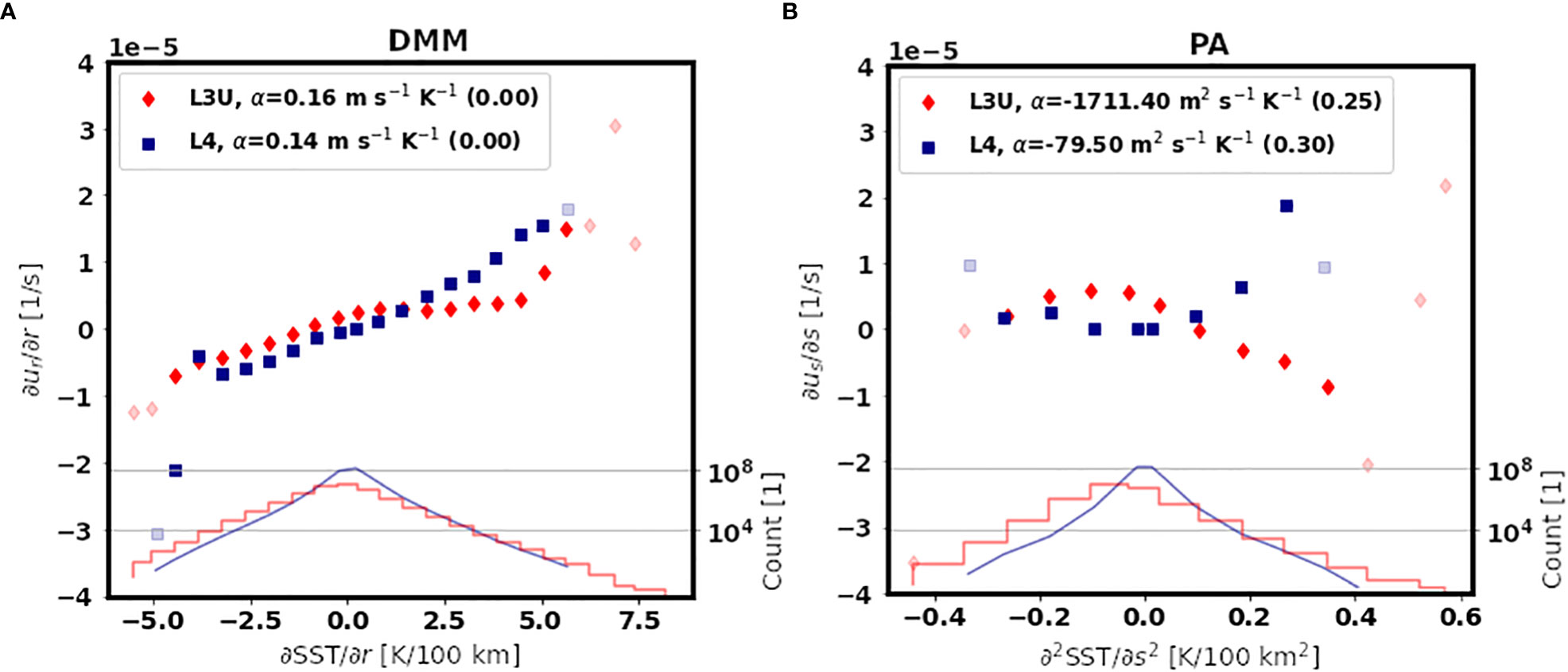
Figure 9 Binned scatter plots of (A) along-wind SST gradient (∂SST/∂r) and along-wind wind divergence (∂ur/∂r), and (B) across-wind SST Laplacian (∂ 2SST/∂s2) and across-wind wind divergence (∂us/∂s). Transparent symbols indicate that less than 100 values were considered in the corresponding bin. In the lower part of the figure, the histogram of the forcing SST fields are shown. The legend contains the linear regression slope of the scatter plots denoted as α and its p-value in parentheses.
Keywords: Air-sea interactions, north-west tropical Atlantic, ocean fine-scale, marine atmospheric boundary layer, coupling coefficients, latent heat flux downscaling, latent heat flux sensitivity to SST
Citation: Fernández P, Speich S, Borgnino M, Meroni AN, Desbiolles F and Pasquero C (2023) On the importance of the atmospheric coupling to the small-scale ocean in the modulation of latent heat flux. Front. Mar. Sci. 10:1136558. doi: 10.3389/fmars.2023.1136558
Received: 03 January 2023; Accepted: 13 February 2023;
Published: 14 March 2023.
Edited by:
Jinbao Song, Zhejiang University, ChinaReviewed by:
Riccardo Farneti, The Abdus Salam International Centre for Theoretical Physics (ICTP), ItalyCopyright © 2023 Fernández, Speich, Borgnino, Meroni, Desbiolles and Pasquero. This is an open-access article distributed under the terms of the Creative Commons Attribution License (CC BY). The use, distribution or reproduction in other forums is permitted, provided the original author(s) and the copyright owner(s) are credited and that the original publication in this journal is cited, in accordance with accepted academic practice. No use, distribution or reproduction is permitted which does not comply with these terms.
*Correspondence: Pablo Fernández, cGFibG8uZmVybmFuZGV6QGxtZC5pcHNsLmZy
Disclaimer: All claims expressed in this article are solely those of the authors and do not necessarily represent those of their affiliated organizations, or those of the publisher, the editors and the reviewers. Any product that may be evaluated in this article or claim that may be made by its manufacturer is not guaranteed or endorsed by the publisher.
Research integrity at Frontiers
Learn more about the work of our research integrity team to safeguard the quality of each article we publish.