 Craig L. McNeil
 Eric A. D’Asaro
 Mark A. Altabet
 Roberta C. Hamme
 Emilio Garcia-Robledo
- 1Applied Physics Laboratory, University of Washington, Seattle, WA, United States
- 2School for Marine Science and Technology, University of Massachusetts Dartmouth, New Bedford, MA, United States
- 3School of Earth and Ocean Sciences, University of Victoria, Victoria, BC, Canada
- 4Department of Biology, University of Cadiz, Cadiz, Spain
Oxygen Deficient Zones (ODZs) of the world’s oceans represent a relatively small fraction of the ocean by volume (<0.05% for suboxic and<5% for hypoxic) yet are receiving increased attention by experimentalists and modelers due to their importance in ocean nutrient cycling and predicted susceptibility to expansion and/or contraction forced by global warming. Conventional methods to study these biogeochemically important regions of the ocean have relied on well-developed but still relatively high cost and labor-intensive shipboard methods that include mass-spectrometric analysis of nitrogen-to-argon ratios (N2/Ar) and nutrient stoichiometry (relative abundance of nitrate, nitrite, and phosphate). Experimental studies of denitrification rates and processes typically involve either in-situ or in-vitro incubations using isotopically labeled nutrients. Over the last several years we have been developing a Gas Tension Device (GTD) to study ODZ denitrification including deployment in the largest ODZ, the Eastern Tropical North Pacific (ETNP). The GTD measures total dissolved gas pressure from which dissolved N2 concentration is calculated. Data from two cruises passing through the core of the ETNP near 17 °N in late 2020 and 2021 are presented, with additional comparisons at 12 °N for GTDs mounted on a rosette/CTD as well as modified profiling Argo-style floats. Gas tension was measured on the float with an accuracy of< 0.1% and relatively low precision (< 0.12%) when shallow (P< 200 dbar) and high precision (< 0.03%) when deep (P > 300 dbar). We discriminate biologically produced N2 (ie., denitrification) from N2 in excess of saturation due to physical processes (e.g., mixing) using a new tracer – ‘preformed excess-N2’. We used inert dissolved argon (Ar) to help test the assumption that preformed excess-N2 is indeed conservative. We used the shipboard measurements to quantify preformed excess-N2 by cross-calibrating the gas tension method to the nutrient-deficit method. At 17 °N preformed excess-N2 decreased from approximately 28 to 12 µmol/kg over σ0 = 24–27 kg/m3 with a resulting precision of ±1 µmol N2/kg; at 12 °N values were similar except in the potential density range of 25.7< σ0< 26.3 where they were lower by 1 µmol N2/kg due likely to being composed of different source waters. We then applied these results to gas tension and O2 (< 3 µmol O2/kg) profiles measured by the nearby float to obtain the first autonomous biogenic N2 profile in the open ocean with an RMSE of ± 0.78 µM N2, or ± 19%. We also assessed the potential of the method to measure denitrification rates directly from the accumulation of biogenic N2 during the float drifts between profiling. The results suggest biogenic N2 rates of ±20 nM N2/day could be detected over >16 days (positive rates would indicate denitrification processes whereas negative rates would indicate predominantly dilution by mixing). These new observations demonstrate the potential of the gas tension method to determine biogenic N2 accurately and precisely in future studies of ODZs.
1 Introduction
ODZ’s are important in ocean nutrient cycling, typically are in close proximity to large fisheries, and are susceptibile to change linked to global warming (Engel et al., 2022). Occurring primarily on the eastern edge of ocean basins, ODZ’s are a recognized source of the potent greenhouse gas nitrous-oxide (N2O) to the atmosphere and an oceanic sink of nitrogen-based nutrients (nitrate and nitrite) as a consequence of microbial processes (denitrification and anammox) requiring the near absence of O2 (Codispoti et al., 2001). Nitrogen cycling activity levels of ODZ microbial communities thus overall have a positive response to the supply of organic matter and a negative response to oxygen despite varying individual responses. The tolerance of anaerobic microbes to trace levels (nM) of dissolved oxygen (O2) has been the focus of many prior laboratory and field studies due to its importance in modeling and prediction. The simplest model (exponential-type inhibition kinetics) assumes a threshold of O2 at or below a few hundred nM O2 (~0.1% of background outside the ODZ) above which denitrification processes resulting in the the accumulation of N2 gas in the mesopelagic stop (Dalsgaard et al., 2014). There is considerable uncertainty associated with this threshold O2 concentration and even the applicability of such a simplified model since microbes can adapt and respond to O2 forcing, so a deeper knowledge of sub-threshold O2 responses is required (Bristow et al., 2016; Garcia-Robledo et al., 2017; Zakem and Follows, 2017; Penn et al., 2019; Berg et al., 2022). Identification of ODZ waters is more commonly based on denitrification activity, rather than oxygen concentration, through removal of (N deficit), the presence of a secondary maximum (Banse et al., 2017), or the appearance of biogenic N2 produced by denitrification. These waters have also been termed ‘functionally anoxic’ having O2 concentrations of<10’s nM (Revsbech et al., 2009; Tiano et al., 2014).
From an experimental viewpoint focused on dissolved gas cycling, the study of ODZ biogeochemistry requires measuring trace level changes in O2 and N2 correlated in time and space with likely forcings. Prior studies of open ocean ODZs have measured water column biogenic-N2 and denitrification rates (ie., the production rate of biogenic-N2) using a combination of mass-spectrometric or gas-chromatographic analysis of dissolved N2 in discrete water samples (Chang et al., 2010; Chang et al., 2012; Fuchsman et al., 2018) or in vitro incubations using automated nutrient analysis for elemental stoichiometry and spiking with 15N-labeled substrates to distinguish denitrification and anaerobic ammonium oxidation (anammox) processes (e.g., Babbin et al., 2014; Dalsgaard et al., 2014). Although these types of measurements are generally highly precise and accurate, they are both costly due to the requirement for specialized collection, storage, and analysis of seawater samples at a shoreside laboratory and limited in time and space. Consequently, large research gaps have developed because of the limited types, quantity, and distribution of oceanographic data provided by existing methods. A few prior studies have investigated spatial variability in ocean denitrification rates and found evidence that eddies can be significant hotspots for denitrification (Callbeck et al., 2017; Altabet and Bourbonnais, 2019) but more statistics are needed to better understand how important eddies really are in ODZ biogeochemistry. Although short term variability in denitrification rates can be measured during a several week-long cruise, investigation of seasonal cycles in N2 using sparse existing data sets collected using conventional approaches is far out of reach. New in situ methods are needed that can be deployed on moorings, floats, and gliders to allow measurement of denitrification at revelvant spatial and temporal scales.
Over the last several years we have been developing new approaches for studying denitrification in the Eastern Tropical North Pacific (ETNP, see Figure 1), the largest of the three major ODZs. Our approach was motivated by the need to autonomously observe long-term changes in dissolved gas cycling within ODZs that have been observed (Horak et al., 2016; Ito et al., 2017), or are predicted (e.g., Deutsch et al., 2014), to occur due to the impacts of global warming on ODZ biogeochemistry. We use a membrane-based dissolved gas sensor known as a Gas Tension Device (GTD), which was originally developed (McNeil et al., 1995) for studying air-sea gas exchange rates and processes in oxic waters, to measure total dissolved air pressure. With the intent of providing enough detail so other researchers can employ these methods for themselves, and likely improve upon them, we describe the dissolved gas sensors and adaptations for the sampling platforms we used, and the assumptions and data processing steps involved in calculating N2 concentrations, biogenic-N2, and even denitrification rates. A limitation of our approach, based on measuring N2 in situ, is that we cannot distinguish different processes that produce N2 gas as other methods, such as labeled-incubations with GC-MS analysis, can and so we cannot distinguish denitrification and annamox processes (unless perhaps these processes are known to occur in different regions of the water column or under different environmental conditions).
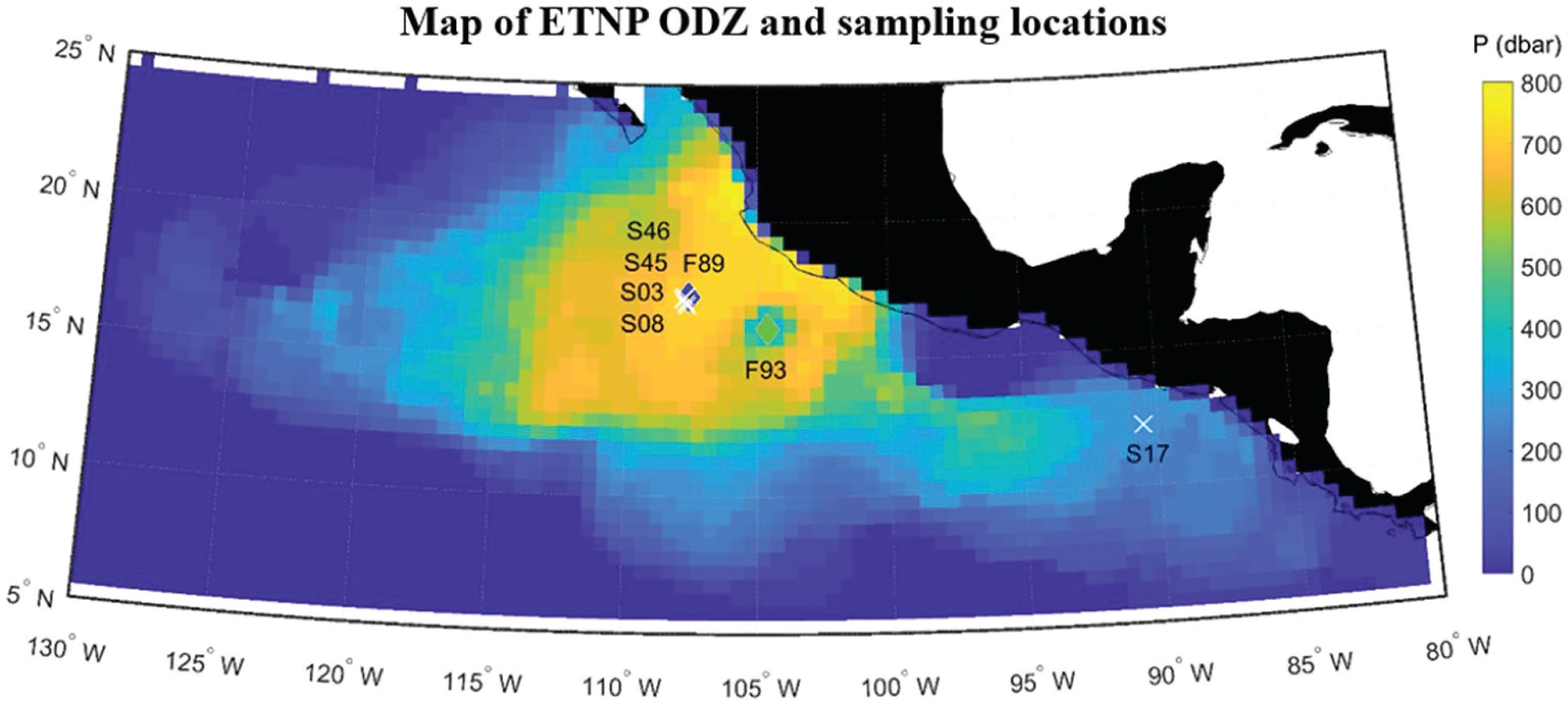
Figure 1 Map of the ETNP showing the thickness (color scale) of the ODZ layer from the reanalysis by Kwiecinski and Babbin (2021) overlaid with the shipboard CTD stations (white crosses labeled with ‘Station#’ from Table 1) and location of the float sampling (‘F89’ – filled blue diamond, ‘F93’ – filled light green diamond).
We present and discuss vertical profiles of GTD-derived biogenic-N2 made using data collected in the core waters of the ETNP near 17 °N. The data highlights that real-time biogenic-N2 can now be measured at sea by ships and BGC-Argo-style profiling floats and therefore this new method offers the possibility to map important oceanographic regions (e.g., ODZ boundary) or study oceanographic features of interest (e.g., eddies) within the ODZ. These data also motive the need to better understand subtler long-term changes in ODZ biogeochemistry through a combination of combined observational and modeling campaigns.
2 Materials and methods
2.1 Overview
To better study ODZ biogeochemistry our sampling objectives were: 1) to measure biogenic-N2 profiles that result from microbial decomposition of nitrogen-based nutrients (nitrate, nitrite, ammonia) in anoxic waters at approximately the same location in the ocean (ie., Eulerian approach), and 2) to measure the time rate of change of biogenic-N2, or the denitrification rate, within the same subsurface water mass moving with the mean flow (ie., Lagrangian approach). The Eulerian approach uses a GTD, mounted either on the ship’s CTD or a profiling float, held at various depths or isopycnals for sufficient time (< 1 day) to equilibrate the sensors and obtain a vertical profile. The Lagrangian approach can be used to estimate in situ denitrification rates by making repeat measurements on a freely drifting float at the same isopycnal to ensure sensors stay in the same water mass for sufficient time (>10 days) to detect a change in biogenic N2. In the ODZ core region where horizontal currents are weak, vertical gradients in biogenic-N2 are much larger than horizontal gradients and a simple 1-D budget model for N2 (see Figure 2) can be used to interpret both sampling approaches. A complication when applying such a simplistic N2 budget is the need to separate biogenic and non-biogenic components (e.g., physical processes including mixing). This complication holds for any technique that budgets N2, regardless of the method used to measure N2 in seawater. For example, Chang et al. (2012) encountered this same issue interpreting N2 measurements made in the ETNP ODZ using mass-spectrometric measurements of N2 and solved the problem by referencing their N2 measurements made inside the ODZ region to background measurements at the same density made outside the ODZ. Their technique further benefited from using measured N2/Ar ratios (the raw measurements of the mass spectrometer) since inert Ar provides essentially an intrinsic reference for abiotic-N2. We adopt and extend this same approach by considering the different source waters to the ODZ core region as importing their own preformed excess-N2 to the ODZ and mixing vertically and horizontally along their pathways to the core of the ODZ. Rather than having to measure dissolved gas levels outside the ODZ as Chang et al. did, we calibrate our biogenic N2 to a concurrent but independent measurement based on nutrient stoichiometry to obtain vertical profiles of preformed excess-N2 in the water mixtures at the ODZ core. The validity of the 1-D model is assessed using conservative mixing lines for independently measured argon.
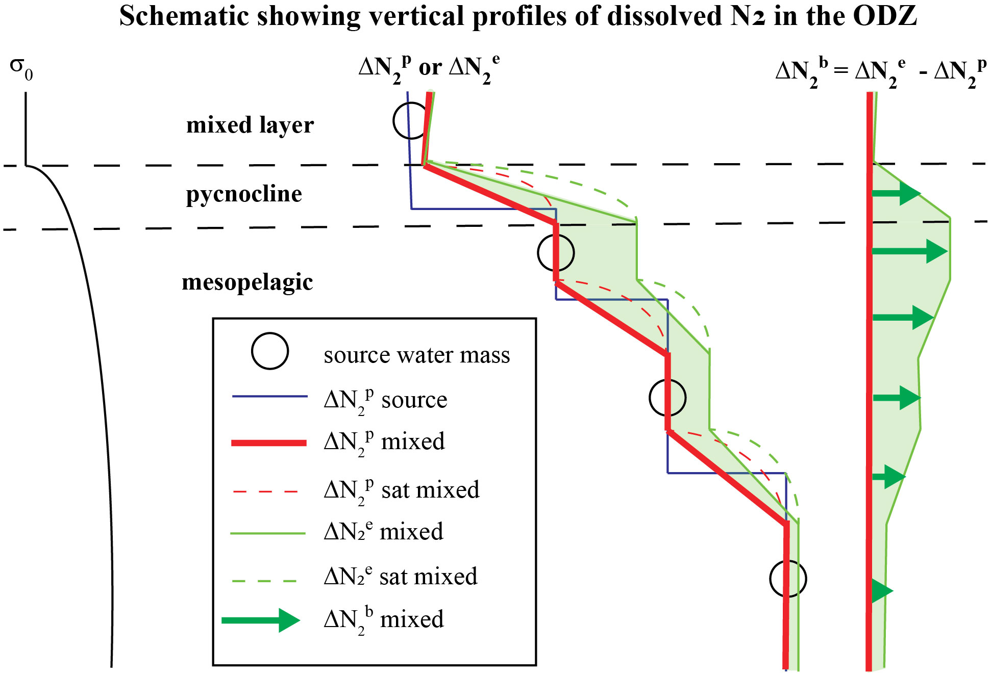
Figure 2 An idealized 1-D schematic of the upper ocean in the ETNP ODZ showing: (left) a vertical profile of potential density σ0, (middle) vertical profiles of preformed excess-N2 ( ) and measured excess-N2 (; ) in layered mixtures of discrete source water masses (circles) that feed the ODZ, and (right) biogenic-N2 ( ) in each layer calculated using Eqn. (4). Discrete source waters (circles) of the ODZ with initial Δ (blue line), set by air-sea gas exchange in the water masses where their isopycnals outcrop and any prior denitrification, mix with each other in the ODZ where they yield a mixed Δ profile (red line). Non-linearity of solubility contributes to supersaturations (see ‘N2 sat’ in legend) of the water mass mixtures. Once a layer becomes functionally anoxic, Δ accumulates in that layer.
We used the in-situ gas tension method as an alternative approach to measuring N2 in seawater since it can be measured autonomously, is relatively easy, reliable, and inexpensive compared to conventional techniques. In the anoxic seawater layer found at the core of the ODZ, the gas tension method has increased accuracy due to the elimination of measurement errors associated with dissolved O2. One prior study used this same advantage to study aerobic/anoxic N2 cycling in the Baltic Sea (Loeffler et al., 2011). A disadvantage of the gas tension method alone is that argon levels are usually assumed, and therefore no compensatory information on abiotic processes is measured. We, however, used an advanced isotope dilution mass-spectrometric technique developed to measure absolute Ar concentrations to high accuracy. The Ar samples were drawn from the same rosette CTD used for gas tension sampling. The drawbacks of the isotope dilution technique method are high per-sample analysis cost and there are only a few laboratories that can do it, but this disadvantage is somewhat offset by the fact that argon is expected to vary predictably and smoothly (Ito et al., 2011) by conservative mixing away from boundary sources so only targeted sampling of ODZ source waters was required. We used independent shipboard measurements of biogenic N2 from nutrient stoichiometry with concurrent gas tension derived estimates of biogenic N2 to determine N2 variability due solely to physical processes. We used the Ar measured by isotope dilution techniques to check our assumption that this ‘preformed’ excess-N2 followed expected conservative mixing curves. We applied the preformed excess-N2 profiles measured in the ODZ core during the cruise to profiles of gas tension measured after the cruise by autonomous profiling floats deployed in the same vicinity to obtain the first autonomous biogenic N2 profiles in an ODZ. Derived denitrification rates require a quantifiable increase of biogenic N2 within the same water mass over a known period of time; this period will be longer for regions or isopycnals with lower microbial activity.
2.2 Field campaigns
Biogenic N2 was measured in the ETNP near 17 °N (see Figure 1) during two cruises on the RV Sally Ride (CruiseID = SR2011 during 16-Dec-2020 to 06-Jan-2021m; CruiseID = SR2114 during 21-Dec-2021 to 21-Jan-2022). A GTD was mounted on the rosette CTD to measure vertical profiles of gas tension, along with O2 (by SBE-43), temperature (T) and salinity (S). Water samples were taken for nutrients (nitrate, nitrite and phosphate). A Switchable Trace amount OX-ygen (STOX) sensor (Revsbech et al., 2011) was used to reference the SBE-43 O2 data to anoxia (± 50 nM) in the ODZ core waters. Autonomous floats, also with GTD sensors, were deployed. Table 1 lists sampling details for the data presented here.
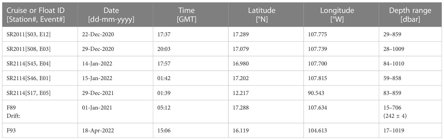
Table 1 Details on time, location, and depth range of GTD sampling by ship and float.
2.3 Gas tension devices
New versions of Gas Tension Devices (GTDs manufactured by Pro-Oceanus Systems, Inc., Bridgewater, NS, Canada) were used to measure gas tension on the floats and the ship’s CTD in this study. Unlike older versions of the GTD (McNeil et al., 1995; McNeil et al., 2006), the new sensor has only a weak hydrostatic response, due primarily to the use of the relatively incompressible Teflon AF 2400 gas permeable membrane introduced by Reed et al. (2018). The new GTD has the same external mechanical design as the profiling GTD developed for use on the ship’s CTD (McNeil et al., 2018, see figures on pages 88 and 96) but was modified at APL/UW internally to: 1) improve the electronics, and 2) allow the sensor’s pressure sensor to be easily replaced at sea even in the event of a flooded membrane. The novelty of the profiling GTD design lies in the use of a miniature pressure sensor (type Micro Electrical Mechanical System- or MEMS) with a very small (approximately 40 µL) gas sensing volume. Since this pressure sensing volume contributes to the total sample volume behind the membrane that must exchange through the membrane, the response time of the new GTD is small: In separate laboratory tests conducted using similar high-flow pumps and plenums the characteristic (e-folding) response times were approximately 1 minute at 20°C and 3 minutes at 5 °C. The response time of any GTD varies with seawater temperature because of the temperature dependence of gas diffusivity and solubility in the GTD’s membrane. The new GTD was mounted onto a rosette 911 SBE CTD system that had a serial RS-232 (‘Data Uplink’) capability for real-time data and a spare SBE 5T pump running at approximately 50% of maximum capacity (ie., 0.5 A at 12 V, or 6 W); the pump flushed the GTD’s membrane using a plenum attachment as described in McNeil et al. (2018). The GTD had an operating-depth rating of 1000 m.
The time required to equilibrate the new GTD to an acceptable level (e.g.,<1 mbar of absolute) when profiled through strong temperature and dissolved gas gradients is not simply a function of the isothermal response time of the sensor found in the laboratory, it also depends on the prior history of exposure of the sensor during the profile and geophysical noise such as the passage of internal waves. Since GTD measurements took many hours on station, it was necessary to minimize the wait time at each sampling depth and provide a straightforward procedure for CTD operators to follow. At-sea trials of the new GTD on the ship’s CTD were performed at the start of the cruise to determine the minimum wait-time required to equilibrate the GTD in temperature and gas before moving the CTD to the next sampling-depth. A wait-time of 10 minutes at each sampling-depth found to be sufficient except in the thermocline where the wait-time was increased to 15 minutes. Equilibrated data were chosen based on averages over the last few minutes of data prior to moving the CTD to the next depth.
2.4 Autonomous floats
As part of a larger distributed array designed to capture relevant temporal and spatial variability in denitrification rates and processes in the ETNP, a total of 10 modified Argo-style floats were deployed on the two cruises and data from two of those floats deployed in the ODZ core region are examined here. Floats (model ALTO) manufactured by Marine Robotics Systems (MRV) were modified in collaboration with MRV to carry one or more GTD sensors and two Seabird-63 optode oxygen sensors. The float’s new GTD and optode membranes were flushed using a low flow rate SBE-5M pump to reduce power consumption, the trade-off being a significantly longer equilibration time of approximately 20 minutes for the GTD (ie., approximately 20 times slower than the fastest laboratory equilibrations). One of the two optodes measured the water; the other measured in a saturated sodium sulfite solution and acted as an anoxic reference solution subject to the same temperature and pressure as the water optode. The standard optode calibration equation is not accurate at concentrations below a few µmol/kg as it does not account for temperature and pressure dependences of the optode response at zero oxygen. Here, oxygen was computed both from the difference between the water and reference optodes corrected for a linear pressure trend and by reformulating the calibration equation with the appropriate pressure and temperature variations. The ODZ core was clearly apparent as a minimum in oxygen concentration several hundred meters thick, with values of a few µmol/kg or less and a linear variation of oxygen with depth of a few hundred nmol/kg. The pressure coefficient was adjusted to make oxygen constant in this region; an offset was adjusted to center this on zero. The STOX sensor on the ship’s CTD, when available, was used to check the optode derived profiles. A detailed description is beyond the scope of this paper and will be reported elsewhere.
The float mission was modified from that of a standard Argo float. After an initial dive to 800–1000 m and a few hours to allow the sensors to settle, the float profiled upward in a stairstep profile (Figure 3), moving upward 50–100 m, then settling at a nearly fixed depth and isopycnal for 1–2 hours to allow the GTD to equilibrate, then moving upward again. The float then drifted for up to 10 days in the OMZ just below the oxycline, about 200 m, before continuing the stair-step profile upward, surfacing, communicating, and repeating the cycle. Occasional glitches resulted in the float profiling to as deep as 1500 m with no apparent issues.
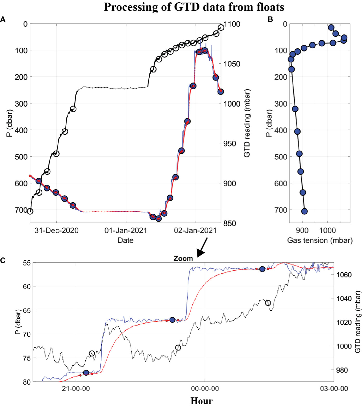
Figure 3 Example of raw and processed float data, from F89, showing: (A) Time series of hydrostatic pressure (left axis, black line) with time marks showing when the GTD is fully equilibrated (left axis, black circles), raw GTD reading (right axis, red line), and deconvolved GTD data (right axis, blue line), with time marks (small red dots) over which the mean equilibrated gas tension is calculated (large blue dot); (B) Vertical profile of gas tension (large blue dots); and (C) Zoom-in of the upper plot for three equilibrations, starting at 20:00 on 01-Jan-2021.
Data from two floats are reported here. The first float (F89) was deployed in the ODZ core close to the location of four CTD stations (S46, S45, S03, S08) occupied during our two cruises (see Figure 1). Only shipboard data, not all concurrent, were used to calibrate our new method for determining biogenic N2. After calibrations, our new method was then applied to the float data to provide the first test of the new method when applied to autonomously collected data delivered by satellite. Since the first float and CTD data were collected at the same location within the ODZ, the comparison is designed to provide information on the accumulated errors when applying our new method to float data. To demonstrate our overall goal of a long-term distributed float-based sensing observational system, we applied our new method to data from a second float (F93) chosen to be nearby and longafter the shipboard calibrations work.
2.5 Dissolved N2 from gas tension
Definitions - Dissolved N2 partial pressure (pN2) was calculated by the gas tension method using:
where PT is the total gas tension, and pO2 and pH2O are the partial pressure of oxygen and water vapor, respectively. The trace gas partial pressure (pTrace) is mostly argon with a small contribution from pCO2, is relatively small, and can be accounted for in the calculations with little error (using Table 1 from Reed et al., 2018 we expect pTrace = 9.6 – 10.9 (± 0.9) mbar for P = 0 – 400 dbar, which is equivalent to an uncertainty of ± 16% in an assumed biogenic N2 signal of 10 mbar). It should be possible to reduce uncertainties associated with pCO2 further (we did not measure it) by estimating it from either Apparent Oxygen Utilization (AOU) or climatological empirical relationships for carbonate system parameters within the ODZ (i.e., TAlk and DIC versus temperature and sailinity) along with the standard seawater carbonate system calculators (e.g., CO2SYS program). We have not attempted to include any corrections here since our initial focus was understanding large scale variability in pN2 associated with variability in actual preformed N2. We refer to the calculated dissolved nitrogen concentration using Henry’s Law and Equ. (1) as the ‘measured’ nitrogen ():
where gas specific Henry’s Law solubility coefficients (SH) are known functions of water temperature (T), salinity (S), and hydrostatic pressure (P). Unique to the ODZ is a functionally anoxic core layer where pO2 = 0. Outside of this anoxic layer small changes in O2 are accounted for in Eqn. (2) with little error in determined N2 by referencing the O2 sensor data from the ship’s CTD to a precise zero-point using a STOX sensor (more details below - see also Supplement in Tiano et al., 2014). We refer to nitrogen ‘solubility’ () as the value in seawater in equilibrium with one standard atmosphere of moist tropospheric air (Hamme and Emerson, 2004). All Henry’s Law solubilities are calculated using MATLAB solubility calculators (Emerson and Hamme, 2022).
We define other nitrogen quantities as well, specifically ‘excess’ nitrogen (Δ ) as:
and ‘biogenic’ nitrogen (Δ ) as:
where the ‘preformed’ excess nitrogen ( ) is the portion of excess N2 associated with all processes that alter source water N2 prior to it entering the ODZ, and include: 1) physical (abiotic) processes, such as air-sea gas exchange of the water masses during formation, and 2) denitrification in anoxic micro-environments of sinking organic matter (Bianchi et al., 2018) or continental shelf sediments (Devol, 2015). Since each source water mass to the ODZ will have its own value of Δ with likely small interannual variability since the water formation regions are remote, we can expect mixing of the source waters within the ODZ to create stronger spatial than temporal variability in Δ throughout the ODZ. Conservative mixing of two source waters that have different T and Δ raises the N2 saturation level of the mixture, a consequence of the non-linearity in the temperature dependence of Henry’s Law solubility coefficients (rather than production of N2) and must be accounted for in all mixing calculations.
Deconvolutions – To determine equilibrium values of measured quantities on the floats, which have a much slower response GTD than used on the ship CTD due to available power, we used a deconvolution model similar to Reed et al. (2018) with a suitable intrinsic (e-folding) response time scale determined by inspection of the raw data. We applied this deconvolution model to determine both raw quantities (e.g., gas tension) and derived parameters (e.g., Δ ). Initial transients can result from the fact that O2 rapidly leaves the GTD after it was lowered into the deeper anoxic waters from the equilibrated sea surface while at the same time N2 entered the GTD because N2 was supersaturated in the deeper anoxic core waters due to denitrification processes making modeling of the float data difficult. To accurately deconvolve all the raw gas tension signal required use of a multiple response time deconvolution model that separately tracked equilibration of each gas. Although we developed and tested this more complex deconvolution approach, we avoided using it by simply neglecting initial transients in the derived quantities (manifest as overshoots in the raw data) and determining equilibrium values for the later phase of equilibration since the additional complexity in the end added no value to the results based on the goal of determining equilibrium end-points. However, we add this information here to document that more complex details GTD equilibration in the ODZ can be understood if, for some reason, that were an objective of the analysis. By design, the thermal equilibration time of the GTD is smaller than the gas diffusion equilibration time scales (for N2 and O2) so thermal transients mostly relax quickly. This much simpler approach worked well under most circumstances, except during profiling across the strongest part of the thermocline and the only solution to that problem was to hold the sensors for longer at those depths before moving the sensor to the next sampling depth as described above.
2.6 Biogenic N2 from nutrient deficit
We use the nutrient deficit (Ndef) method (Codispoti and Richards, 1976; Codispoti et al., 2001) to calculate an independent ‘nutrient’ ( ) based on the stoichiometry of microbial N2 production from nitrate. Ndef is the difference between measured and expected dissolved inorganic nitrogen (DIN) concentrations with DIN as the sum of measured and as is typically undetectable in the open ODZ:
where the divisor α accounts for conversion to di-nitrogen (N2) gas using appropriate stoichiomentry.
DINexp is commonly estimated from given its strong linear relationship with outside of ODZ’s. Here we use regression coefficients to estimate DINexp derived from data in the GLODAP V2 database for regions adjacent to the western Mexico EDZ:
The slope and intercept for Eqn. 7 was determined through linear regression of data from the GLODAP database (Garcia et al., 2014) for the ETNP region excluding points with evidence of denitrification with results similar to Chang et al. (2012). For these calculations we used α = 2.0. , , and were measured on board using a SEAL AQ 400 nutrient analyzer using standard methods. was also estimated via a linear regression with AOU data also using the GLODAP database. This approach was applied to the 12°N station, and one station at 17 °N, as data quality problems with the directly measured data was evident. For those calculations, α = 1.712 was used following the stoichiometry of Richard’s equation: (CH2O)106(NH3)16H3PO4 + 94.4 HNO3 = 106 CO2 + 55.2 N2 + 177.2 H2O + H3PO4 (Richards, 1965).
2.7 Conservative preformed excess N2
Equating the measured biogenic-N2 derived from the GTD-method (i.e., Δ from Eq. 4) to that measured by the nutrient-method (i.e., Δ from Eqn. 6) using our CTD station data - even if the CTD stations were from inside of the ODZ region as will be discussed in Section 2.9 - we obtain a measurement-based estimate of the preformed excess-N2 from:
By interpolating (on density) the shipboard measurements to common density levels, we derived vertical profiles of Δ at the ODZ core. Measurements were made at approximately the same latitude (17 °N), in duplicate casts, and repeated one year later (see Table 1) to assess interannual variability. Argon and nutrients were typically measured at the same CTD station on the prior or next cast that the GTD measurements were made due to sampling limitations but Argon data are only available here for the first cruise (samples were collected during the second cruise but analysis is not yet complete).
In the deeper stratified waters of the ODZ, which is unaffected by air-sea gas exchange processes, we expect Δ to be a conservative quantity. We also expect latitudinal variability in Δ since the ODZ core is fed by multiple northern and southern sources, and each source water having been formed in different regions of the ocean will likely have different Δ . An objective is to reliably predict Δ across the entire ODZ based on circulation and conservative mixing of ODZ source waters then use those predicted distributions along with measured profiles of gas tension, temperature, salinity and oxygen to predict, using Eqn. (4), biogenic N2 at the floats. We assess latitudinal variability in Δ comparing estimates made in the ODZ core at 17 °N to measurements made at 12 °N which are strongly influenced by the southern sources. Since these two stations capture a large fraction of the variability in the ETNP ODZ hydrography, we expect the comparison to provide a first look at how variable Δ is within the ETNP ODZ for different source water masses. Finding no differences in the deeper water masses below the active denitrification zone would be a good internal-consistency check of our methods, noting that we cannot independently verify our method without a second independent measurement of Δ .
2.8 In situ denitrification rates
Measurements of N2 made on a float following a subsurface water mass (Lagrangian) in theory allow in situ production (or consumption) rates to be determined by measurement of dN2/dt if horizontal (isopycnal) and vertical (diapycnal) mixing effects are fully compensated. However, floats do not follow water masses perfectly, especially if the water mass properties change over time due to vertically sheared mixing which will dilute over time the original water mass under study with the surrounding waters. Notwithstanding these complications, local denitrification rates (DNR) along the float track-line can be estimated from the production of biogenic N2 at the float using:
Note that for a perfectly Lagrangian float with negligible vertical fluxes of biogenic N2 or preformed biogenic N2, the term Δ in Eqn. (9) could be replaced by Δ .
2.9 Argon measurements and assumptions
Although argon is a small component of the gas tension signal and assumptions for argon have little impact on the biogenic N2 error analysis (see Section 2.4), argon still plays a significant role in our work as a proxy measurement of inert-N2 which, theoretically, would be a fully conservative quantity in the ODZ mesopelagic. Since we cannot measure conservative Δ everywhere in the ODZ, we use argon to help predict distributions of Δ based on the stirring and mixing of source waters within the ODZ. We capitalize on the fact that argon, like potential temperature and salinity, is a third conservative tracer and therefore expect Ar and Δ to co-vary.
Source waters for the ODZ were last at the ocean surface outside the ODZ, likely during periods of strong air-sea interaction. During water mass formation, local atmospheric pressure may be several percent different from one atmosphere and rapid cooling may have caused further disequilibrium in gas saturation levels, but these processes affect N2 and Ar similarly (Stanley and Jenkins, 2013; Hamme et al., 2019). Dissolution of bubbles from breaking waves also creates gas supersaturation, at nearly twice the rate for nitrogen as for argon due to their differences in solubility. However, given that both preformed excess N2 and argon are inert and conservative, we expect variability in these quantities within the ODZ to be relatively small and to vary smoothly over large spatial and temporal scales in similar ways. Precise Ar concentrations can only be measured using advanced mass-spectrometric techniques (e.g., isotope dilution, see Section 2.9) and there are only a few existing measurements in the ETNP. Prior studies did not specifically target measurements in the ODZ source waters.
One particularly relevant study of the ETNP region (Chang et al., 2012) derived a relationship for the gas concentration ratio Ar:N2, which is much easier to measure than argon alone, as a function of potential density and geographically separated into ‘inside’ and ‘outside’ of the ODZ. Their analysis was based on a difference approach, subtracting ‘inside’ from ‘outside’ measurements at the same isopycnal to get estimates of the ODZ impact as a function of density. Extending their approach to consider our definition of Δ , it is unclear how Ar:N2 ratios should vary inside the ODZ, as mass spectrometry cannot discriminate Δ from Δ , and would imply that Δ can only be inferred from gas ratio measurements if those measurements are taken ‘outside’ of the ODZ. This argument is fine but breaks down if the measurements made in waters ‘outside’ of the ODZ were previously exported from the ODZ, which is somewhat unavoidable when sampling unless close attention is paid to currents and the history of the current pathway is known when sampling. Also, Chang et al.’s data were collected mostly in the northern waters, which contains information on only half of the ODZ region. Further, their smoothed density relationship derived from ‘outside’ ODZ measurements blurs important information related to mixing of source waters (ie., ‘spice’) which is important evidence for an analysis based on conservative mixing. Combining and replotting all available argon concentration data from Chang et al. (2012) and Fuchsman et al. (2018) showed very clear linear mixing lines, similar to T/S, which convinced us that there was potential for better parameterizations of Δ rather than density alone. Here we argue that the Chang et al.’s approach can be fundamentally improved by focusing attention on the handful of northern and southern source waters to the ODZ, rather than ‘outside’ ODZ waters, and how these source waters get mixed within the ODZ to form ‘inside’ waters. Our approach essentially intensifies the geographical constraints of the problem to the source waters, and demands new data in the southern waters. Our cruises tracks specifically targeted sampling of northern and southern water mass sources to the ODZ and measured argon in them. Most importantly, our improved approach does not require the measurement over all density ranges of ‘outside’ ODZ waters because our conservative mixing model can recreate ‘inside’ and ‘outside’ ODZ mixtures from water mass fractional composition analysis of source waters.
Our argon concentrations were measured by isotope dilution on discrete water samples (Hamme and Severinghaus, 2007; Hamme et al., 2017) collected on the first 2020 cruise. Briefly, glass flasks with a ~180-mL volume and a double-O-ring Louwers-Hapert valve were evacuated to a high vacuum prior to shipping to the field site. The necks of the flasks were kept evacuated by a rough vacuum pump on a large manifold at sea to prevent air leaking into the flasks. Duplicate water samples were introduced from Niskin bottles into the evacuated flasks through tubing pre-flushed with CO2 until the flasks were half-full. Back on shore, flasks were weighed, the headspace and water were equilibrated and then the water was removed. Headspace gases were flowed through ~90°C ethanol to remove water vapor, gettered to remove all except noble gases, an aliquot of 38Ar added, frozen into a tube immersed in liquid helium, and brought to higher pressure with a balance gas of helium. Argon isotopes were analyzed on a dual-inlet MAT 253 Isotope Ratio Mass Spectrometer at the University of Victoria against a standard of similar composition. The standard and 38Ar aliquot amount were calibrated relative to air measurements. The pooled standard deviation of the duplicates for Ar on this cruise was 0.21%.
2.10 Linear Mixing model
To aid interpretation of our station data at 17 °N in the core waters of the ODZ, a linear mixing model was developed based on the five major water types for that region. The model was initialized using shipboard observations of the three conservative tracers, namely potential temperature, salinity and argon concentration. Although argon saturation level is not conservative, it’s strong sensitivity to the choice of water types values helps fine tune the model to best match the observations – this sensitivity comes from the temperature and salinity dependence of the Henry’s Law solubility coefficients. Unlike argon, nitrogen gas is non-conservative in the ODZ due to N2 production by microbial activity in functionally anoxic waters. The abiotic component of N2, which is equivalent to the red line in Figure 2, cannot be measured directly but can be modeled using the calibrated mixing model with conservative preformed excess N2 from Eqn. 8 as inputs.
To determine conservative property values for each water type, a ‘broken-stick’ best fit model was initially applied to the TS data and then to argon concentration. A segmented linear regression (or ‘broken-stick’) routine called SML (Shape Language Modeling) and developed in MATLAB was used with unconstrained setting (ie., ‘free knots’) to find the location in T-S space of the four water type values. These values were then used in the linear mixing model. The process was repeated for argon and salinity then water type values for each conservative property were further refined by tuning the model to fit all observations, including argon saturation levels, simultaneously. The entire process proved too complicated to fully automate, so the values reported here are approximations derived ultimately by visual best fit between the model and the data.
Once the model is best fit to the observations, the model provides a convenient way to determine smoothed versions of any quantity (e.g., of Δ or Δ ) versus potential density that satisfies the model’s conceptual framework (ie., dilution of 5 water types). The results at 17 °N were then compared to results at 12 °N.
3 Results
3.1 Gas tension
An example of raw and processed time series data from an early float (Table 1, F89) mission are shown in Figure 3A. After the float sunk to its maximum depth (700 m) it slowly ascended to the sea surface, stopping at many (17) targeted depths (or isopycnals) to equilibrate the GTD. The wait time at each targeted depth was 2 hours but this was extended to 24 hours at the ‘Lagrangian drift’ depth (242 ± 4 m) on this dive. The total submerged time was approximately 2 days. Data were reported by satellite after surfacing. A constant e-folding response time of 20 minutes was used to deconvolve these raw GTD data (see Figures 3A, C and compare red and blue lines). This is a factor of 10–20 times slower than the fastest response of the sensor achievable using a fast flow rate pump but draws little energy from the float’s batteries since it uses a small flow rate pump. The equilibrated gas tension values at each hold-depth used a 15-minute average of the deconvolved time series just before the float is moved to the next hold-depth. The standard deviation, SD, of the data during the 15 min averaging period provides a good indicator of uncertainty. We found for P > 300 dbar that SD< 0.03% and for P< 200 dbar that SD< 0.12% (see Figure S1 in Supplementary Materials). Internal waves in the strongly stratified thermocline of the ODZ were the leading cause of geophysical noise.
Processing of the shipboard data was much simpler and didn’t require deconvolving the raw data because the hold time of the GTD at any depth (10–15 minutes) was chosen to be much longer than the sensor response time (2–3 minutes, using the high flow rate pump). The noise level of the raw ship GTD data was better than ±0.2 mbar and the end-point detection typically within ±0.5 mbar assessed by variability from steady readings (see Figure S2 in Supplementary Materials).
To summarize, vertical profiles of gas tension (see Eqn. 1), temperature, salinity and dissolved O2 were made at 12 °N and 17 °N by ship and floats during two cruises. Additional processing produced estimates of dissolved N2 (see Eqn. 2), the results of which are described next.
3.2 Regional water mass analysis
Shipboard measured θ, S, Ar, and GTD-derived N2 at the ODZ core near 17 °N are shown in Figure 4. Five regional water types are readily identified on the conservative θ-S diagram (Figure 4A, red dots) as ‘break-points’, defined where the slope of the plot changes rapidly. In theory, any water mass, or layer in this stratified system, that lies between two water types on the θ-S diagram can be described as a mixture of two adjacent water types. The linear mixing model (see Section 2.10) recreates all possible mixtures of water types that could occur between adjacent water types to produce the model result (Figure 4A, red line). The model can only produce straight lines between water types when quantities are conservative, such as θ, S, and Ar. The model easily reproduces the same ‘broken stick’ shape for conservative Ar (Figure 4B, solid red line) that matches the shipboard data. Derived model quantities that are non-conservative can also be calculated from the conservative model output. Gas saturation levels are one such calculation. Since Henry’s Law solubility coefficients are non-linear functions of θ and S, a model Ar saturation level is calculated using the modeled θ, S, and Ar. Since Ar saturation level is non-conservative, the model produces curved lines between water types on a conservative plot and also on density (see Figure 2). The model Ar saturation level reproduces the observed Ar saturation level curved-shape (Figure 4B, semi-transparent red dashed line) and, as mentioned in Section 2.10, is sensitive to the choice of end-member values and provides an additional constraint for tuning the model to the data.
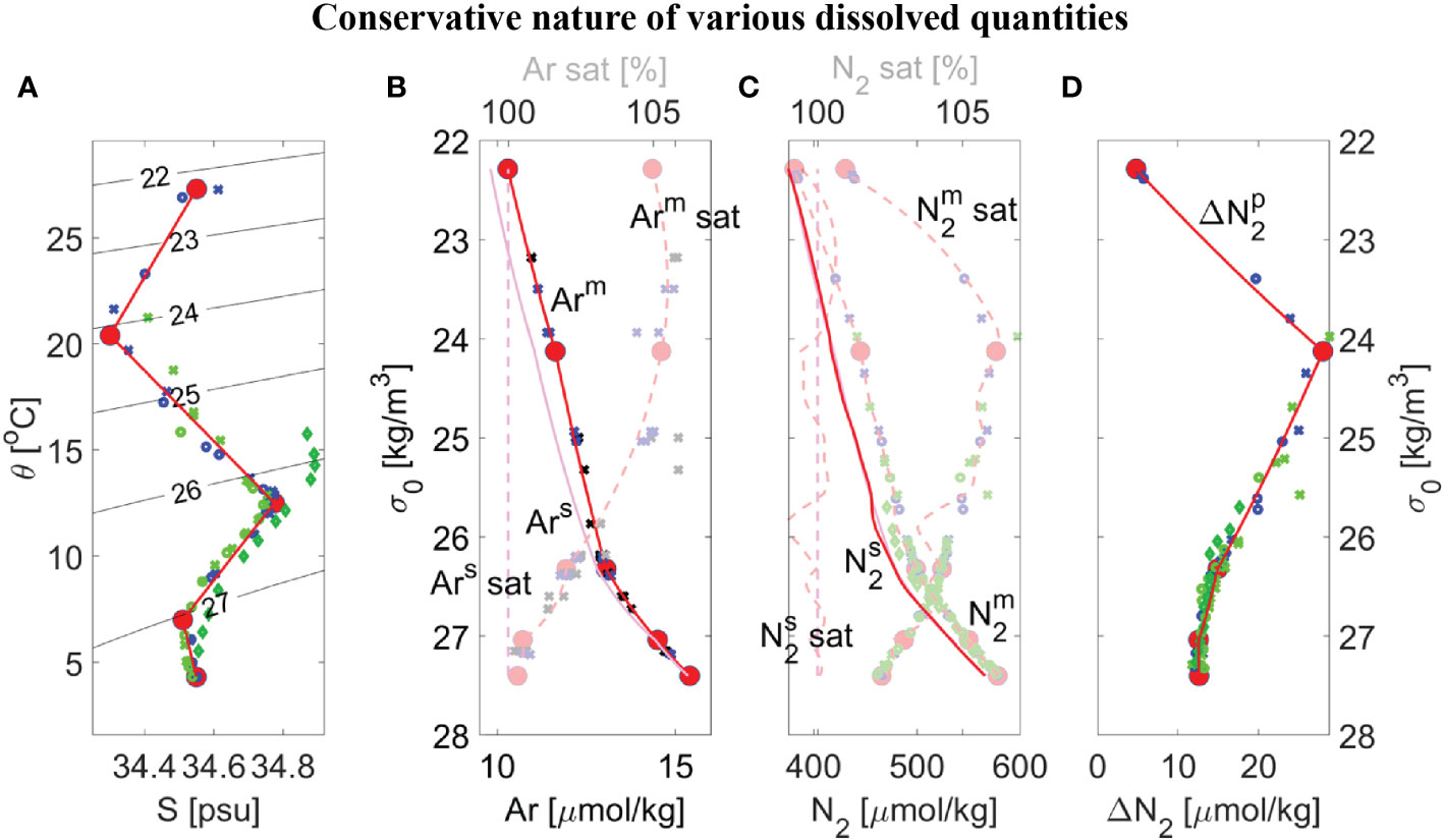
Figure 4 Overview of dissolved gas measurements made during duplicate casts (#1 as small circles, #2 as small crosses, and consistent with Legend shown in Figure 5B) and modeling results (red lines) for either conservative properties (opaque markers and lines) or non-conservative properties (semi-transparent markers and lines) within the ETNP ODZ core near 17°N from SR2011 (blue) or SR2114 (light green) and 12 °N from SR2114 (dark green), showing: (A) Potential temperature θ versus salinity S with contours of potential density σ0; (B) Dissolved argon concentration Arm that is either measured (blue/green symbols) or is a best-fit or mixing-model result (red solid lines), equilibrium solubility Ars (magenta lines), and corresponding saturation level Ar sat (dashed lines) versus potential density σ0; (C) Similar to panel B but GTD-measured nitrogen and best fit (semi-transparent red line) using a smoothing spline with a residual rms of ±0.15% to maintain consistency with errors in solubility coefficients; (D) Preformed excess nitrogen Δ versus σ0 calculated using Eqn. (8). Five distinct water masses (large red dots) were chosen from panel A for the mixing model and all properties were determined by interpolating on potential density to the data. For comparison purposes, corresponding θ/S/Δ at 12 °N from SR2114 were added to panels (A, D) (dark green diamonds) and additional argon data at 14–15.5 °N from SR2011 were added to panel (B) (black markers).
The now calibrated model is used to test the assumption that excess pre-formed N2 derived from the GTD-measured N2 (Figure 4C) is conservative. The model Δ versus σ0 (Figure 4D, red lines) shows breakpoints in density that correspond well with equivalent breakpoints on both θ-S and Ar curves which used both 2021 and 2022 station data due to the limited amount of calibrated data available. These broad similarities provide corroborating evidence that preformed excess N2 is indeed conservative and values for each conservative property can be estimated for each water type. Based on this result, the water type values can be further refined so that preformed excess N2 also is included in the optimization approach to determine water type properties. Our best estimate of water properties for all five water types is summarized in Table 2 and compared to previously published values (Evans et al., 2020). As previously noted, our results do not use an automated ‘broken stick’ detection algorithm and hence errors in the fits are not fully quantified.
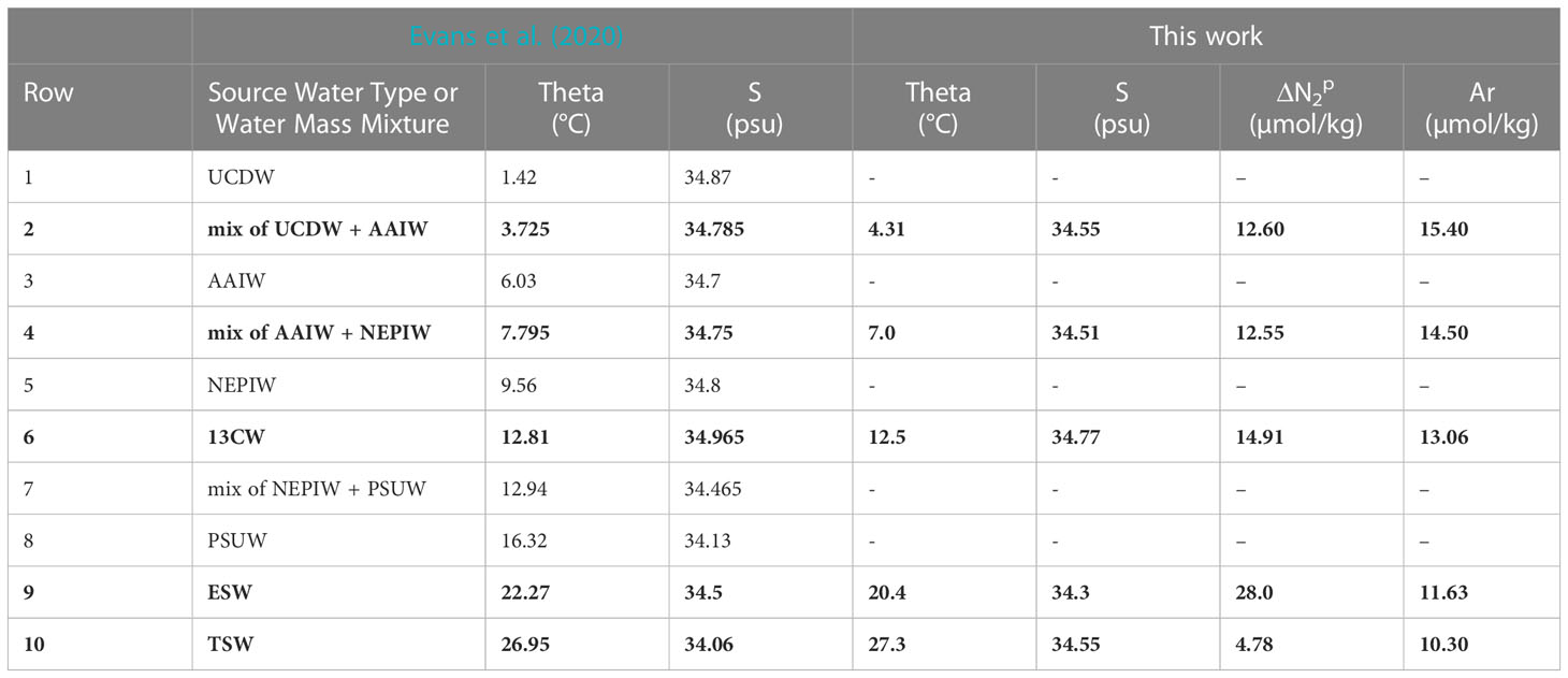
Table 2 Comparison of water types and properties of the ETNP identified by Evans et al. (2020) and water types or water mass mixtures identified in this work (bold text) at 17 °N: Upper Circumpolar Deep Water (UCDW), Antarctic Intermediate Water (AAIW), North Equatorial Pacific Intermediate Water (NEPIW), 13°C Water (13CW), Pacific Subarctic Upper Water (PSUW), Equatorial Surface Water (ESW), and Tropical Surface Water (TSW).
For comparison purposes, additional argon data at 14–15.5 °N from cruise SR2011 were added to Figure 4B to help expand the limited information on argon beyond the site. In addition, corresponding θ/S/Δ at 12 °N from SR2114 were added to Figures 4A, D to provide some additional testing of these new methods. On closer inspection, lower values of Δ , by up to 1 µmolN2/kg, were observed at 12 °N in the potential density range of 25.7< σ0< 26.3 compared to those values at 17 °N indicating water masses (or mixtures of water types) at 12 °N that were not found at 17 °N. Additional evidence is seen on the θS plot (see Figure 4A, dark green diamonds) where these same water at 12 °N are found to have higher salinity than any waters near the same density range at 17 °N. Since it is impossible for the mixing model calibrated at 17 °N to reproduce water masses at 12 °N that have higher salinity than water types found at 17 °N, the anomaly is understandable. Application of the model calibrated to 17 °N to data at 12 °N manifests as a latitudinal dependence to Δ . Considering the regional water masses identified in prior work (Evans et al., 2020), a likely explanation is that we are seeing purer 13CW water at 12 °N than at 17 °N. The obvious solution is to expand the analysis to other latitudes to cover all θ-S space in the ODZ.
In general, all additional data compare favorably with the main results from 17 °N to provide additional confidence that these methods are not simply unique to the core region and have broader applicability over the entire ODZ region, as we would expect given the model framework is based on conservative mixing.
3.3 Biogenic N2 and O2
The model’s best fit of Δ (σ0) at 17 °N (Figure 4D, red line) was then used to determine GTD-derived estimates of Δ using Eqn. 4. This conveniently ensures that any water mass composed of a mixture of two adjacent water types uses the correct and smoothed mixed water mass value for Δ . The results for biogenic N2 alongside O2 are shown in Figure 5. The biogenic N2 peaks at just below the oxycline (within 100 m) at 17 °N. Note that since Δ (σ0) was derived by matching the ship GTD-derived biogenic N2 estimates to the nutrient-derived estimates at 17 °N, the shipboard nutrient and GTD results must agree and the residuals simply provide information on the errors in the data and analysis procedure. A regression fit to a double Gaussian that is constrained to zero at the surface and deepest waters (see Figure 5A, red line) shows an R-squared of 0.96 and RSME of 0.54 µM N2. The first independent float-based measurements of Δ using the same method applied to gas tension and oxygen data from Float 89 within 26 km of the shipboard station generally agrees with the shipboard calibration measurements over 130< P< 630 dbar or O2< 3 uM: Density interpolated measurements show a mean (n=7) difference of -0.42 (± 0.78 RMSE) µM N2, or 10 (± 19) %. This result provides a first quantitative assessment of fully autonomous measurements of biogenic N2 using GTD-equipped floats. ODZ core water O2 near Float 89 was uniform over 160< P< 700 dbar and assumed anoxic since shipboard STOX O2 was ±25 nmol/kg and float optode O2 was likewise near zero and uniform (after correcting for the anoxic optode pressure and temperature coefficients).
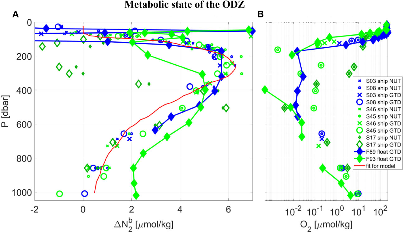
Figure 5 Vertical profiles taken in the core of the ETNP near 17 °N, from SR2011 (blue) and SR2114 (green), of: (A) biogenic N2, and (B) dissolved O2 using a logarithmic scale. Following Table 1 and the Legend, data collected at CTD Station (‘S’) by ship or float (‘F’) used either the traditional nutrient method (‘NUT’) or the new gas tension method (‘GTD’) to measure biogenic N2. Note that all data labeled ‘ship NUT’ are used to calculate the best fit of Δ (σo) so the resulting data labelled ‘ship GTD’ are calibrated and therefore must agree. Data labelled ‘float GTD’ also use Δ (σo) but their gas tension and oxygen are independent. Since ‘F89 float GTD’ data were taken during the cruise and in the vicinity of the float the good agreement serves to validate the GTD method. The ‘F93 float GTD’ data were measured autonomously 2 months after the cruise and much further east (see Figure 1) with significantly different hydrography and are not expected to necessarily agree with ‘F89 float GTD’ data. A second order Gaussian best-fit curve (red line) to the shipboard nutrient data is used for mixing-model calculations.
For comparison to the results from the first float, we present additional measurements made by a second float (see Table 1, float F93) several months after the end of the second cruise and located approximately 350 km to the southeast of the core station. The second float showed lower O2 and higher biogenic N2 in the deeper waters (see Figure 5, float F93 results in light green filled diamonds) consistent with expected higher denitrification rates in less oxygenated waters but less biogenic N2 at comparable O2 in the shallower waters. This could indicate slightly different hydrography between the two locations, with the deeper waters being older at the second float, or variations in denitrification forcing, we don’t know. We also have no independent comparison of Float 93 optode-derived O2 to shipboard STOX due to the fact that the second float data were collected several months after the ship left the region, but expect the absolute value of oxygen is uncertain to several hundred nmol/kg or more. The Δ and O2 profiles from both floats are otherwise fairly consistent which independently supports the results from the first float.
For additional observations with which to compare and contrast with the first float, which was located near 17 °N in the ODZ core, we look to shipboard data from lower latitudes and specifically southern waters which will have different histories of biological processing than those in the core region. Indeed, the largest deviations were observed were near 12 °N where the upper oxycline was much deeper than at the core station with distinctly different water mass properties (see Figure 4A, dark green non-filled diamonds). Remarkably, the same characteristic of biogenic N2 peaking just below the oxycline was reproduced at 12 °N even though the oxycline at 12 °N was approximately 200 m deeper than at 17 °N. Most important, the apparently low Δ values at P = 265 and 305 dbar correspond with significantly high CTD measured O2 (3.6< O2< 6.2 µmol/kg) compared to other mesopelagic waters during the same cast (ie., it likely isn’t a measurement error as the CTD O2 goes well below 1 µM during the same cast) along with observed low and near zero Δ . Since these hypoxic waters are typically considered well above the threshold for functional anoxia, we would not expect these waters to have previously hosted denitrification processes leading to N2 production, leading us to believe these hypoxic waters are the southern source waters we had set out to find. The remaining oxygen in the waters (4.9 ± 1.3 µmol/kg) would need to be lost to respiration processes before becoming functionally anoxic and capable of hosting a robust denitrifying microbial community. This rather exciting discovery also lends support to our overall approach. We also note, however, that no truly independent measurement of biogenic N2 has yet been made at either location and hope to make those measurements in the future.
3.4 Lagrangian drift
An example of various estimates of dissolved N2 variability measured during a 20 hour drift period of a float at a mean potential density of 26.474 kg/m3 are shown in Figure 6. Variability in dissolved N2 (Figure 6, blue line) measured by the gas tension technique is very small, about 1 µmol/kg, or 0.18%. This is comparable to the uncertainty in Henry’s Law solubility coefficients. Variability in biogenic N2 (thick red line) is even smaller, at<250 nmol/kg or<0.05%. The impact of excluding dissolved O2 in the calculation of biogenic N2 is nearly undetectable given that measured O2 variability is at the limit of detection (LOD) and indistinguishable from anoxic conditions. Calculation of rates (Figure 6, black lines) allow trends in Δ to be detected at ±100 nMN2/day: Positive rates would imply active denitrification after compensating for mixing effects and slippage of the float into different waters (which would explain negative rates). These rates and trends seem to be well above the LOD for Δ since internal wave effects with periods of approximately 2 hr are well resolved, implying that longer term averaging (assuming Gaussian distribution) over 16.5 days could reduce these uncertainties to ±20 nM N2/day. This would be suitable for detection of active denitrification in coastal waters of the ETNP where rates of up to 20 nM N2/day have been reported (Babbin et al., 2020), but further resolution would be required to detect active denitrification in the offshore waters with reported rates of up to 4 nM N2/day (Babbin et al., 2020).
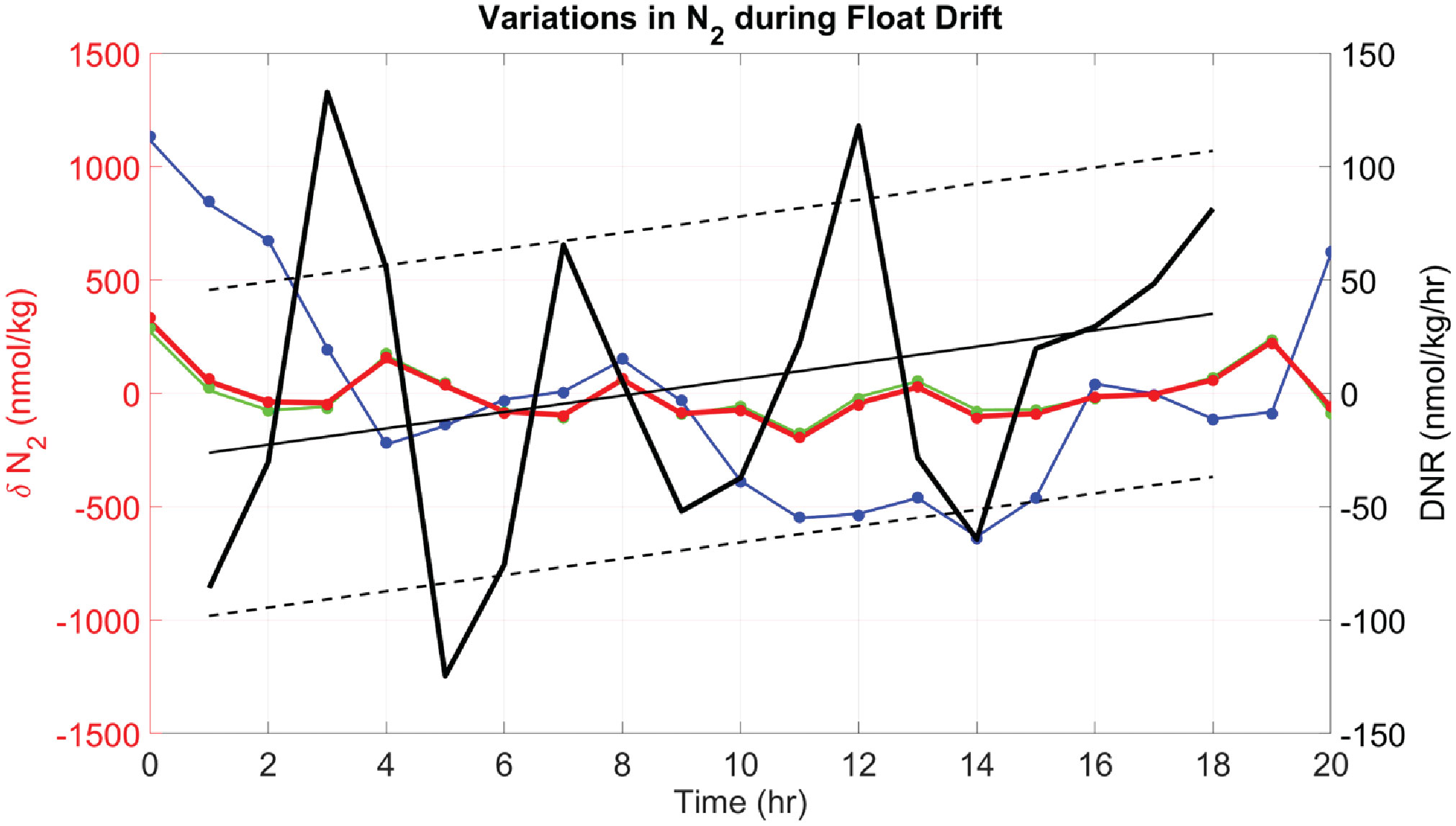
Figure 6 Deviations in water mass N2 from the mean (δN2) during the Lagrangian drift of a float on mean isopycnal of 26.474 kg/m3 and P = 242 ± 4 dbar (F89 starting 31-Dec-2020 at 09:00 GMT). Different calculations of δN2, using a specified ΔN2 and O2, are shown: 1) Δ with measured O2 (red line), 2) Δ with measured O2 (green line), 3) with measured O2 (blue line), and 4) similar calculations as (1) – (3) but assuming anoxia (dots, using same color code). Note that since the plots show deviations from the mean, the mean values of δN2 zero. The Lagrangian rate of change of Δ is shown (left), calculated as local denitrification rate DNR (thick black line) using Eqn. 9, with corrections based on the local vertical gradient. A linear regression fit (thin black line) highlights slowly varying changes in the rates, with ±1 std deviation of the points (black dashed lines) as an indicator of variability. Notice that DNR is negative during the first half of the time series and changes to positive values during the second half of the time series.
4 Discussion
The amplitude (6 ± 1 µmolN2/kg), profile shape, and depth distribution of the biogenic N2 with a peak at 300 m just below the oxycline agree very well with the prior detailed study of Fuchsman et al. (2018) for the ETNP ODZ core. This same study also noted significant and unexplained mismatches in excess and biogenic N2 of 1–2 µmolN2/kg near 15 °N. The authors hypothesized that water mass mixing did not following their empirical ‘background’ (or ‘outside ODZ’) values. Similarly, we found these anomalies at lower latitudes, specially 12 °N, but our water mass mixing approach provides a path toward resolving them. Southern source waters to the ODZ have different preformed excess N2 values at the same density range as waters further north around 17 °N yet span the same density range. A simple density parameterization of ‘background’ excess N2 is thus not sufficient to explain all variability across the entire ODZ. Our approach to reconstruct the equivalent abiotic excess N2 from a mixture of various water types with different preformed excess N2 values should ultimately provide improved biogenic N2 estimates at all latitudes by either method. The relatively small latitudinal dependence of Δ we found by comparing our method applied at 17 °N to observations from 12 °N is expected to be resolved by properly accounting of all water types in the model at 12 °N. Correctly predicting Δ over the entire ETNP ODZ based on a linear mixing model of different water types is an overarching goal.
Our primary nutrient-based estimates of biogenic N2 were used in calibrating our novel gas tension-based estimates, and so a current weakness is the lack of a second independent estimate for comparison. Since many more hydrocasts were taken during both cruises that are not yet fully analyzed, we plan on using these shipboard data at other stations to both calibrate (ie., quantify preformed excess N2) and validate (ie., quantify absolute accuracy). Accuracy and calibration drift is not expected to be limited by the raw measurement of gas tension, although dissolved O2 could introduce comparable errors at either high O2 levels or if the O2 sensor has a significant zero reading offset (>2 µM). To perform the extended analysis over the entire ETNP ODZ and synthesize all our observations, we want to step back and refine a procedure that identifies water types and their values from the ‘broken stick’ analysis of multi-conservative parameter data. Work is in progress to fully automate this procedure with the expectation that the water types and property values can be determined with quantified confidence intervals, a non-trivial task given the fitting needs to be done on scattered data in multi-dimensions with many unconstrained break-points. An alternative approach would be to use a regional numerical model of the ODZ that includes dissolved Ar and a representation of abiotic N2, conservatively redistributes these quantities within the model domain, and is tuned to the observations inside and outside the anoxic core. This would facilitate inclusion of N2/Ar measurements and make better connections between this method and those of Fuchsman et al. (2018) and Chang et al. (2012). The water masses created by mixing of source water types would be subject to parameterization of diapycnal and isopycnal mixing in the model.
Regarding the potential of floats to directly measure in situ denitrification rates (DNR), our first attempt amounts to a test of the procedure given the paucity of the data presented here and the low denitrification rates of the offshore region. It seems clear, however, that improved mapping of Δ and understanding of mixing at the float are prerequisites to inspecting additional data we have collected for scientifically interesting results. There will likely be tradeoffs while trying to reduce uncertainty by using longer averaging periods versus the potential for the float to slip out of the water mass under study and into a different water mass of similar density during the drift. Analysis of longer duration float-drift data is clearly required, but the initial results are encouraging since they suggest that the higher denitrification rates typical of the more productive coastal waters of the ETNP (up to 20 nmolN2/kg/day) should be resolvable using this method by extending the float drift period to more than 16 days. This is a great start.
Lastly, regarding our experiences using the shipboard GTD at sea, we note that each hydrocast took approximately 2.5 hrs longer due to the time required to equilibrate the GTD at the 12 sampling depths – this could be reduced to approximately 1 hr if analysis relied upon deconvolution of the data but more time would need to be spent determining the response time characteristics of the mounted GTD. The same ship’s GTD used on cruise SR2011 was used on the first half of the cruise SR2114 but succumbed to a small crustacean that got trapped in the plenum against the thin membrane and punctured it and had to be swapped out for a spare.
5 Summary
We report for the first time direct autonomous vertical profile measurements of gaseous dissolved biogenic N2 and dissolved O2 made on two profiling floats. The profiles were collected near 17 °N in the ETNP ODZ. The data show peaks in biogenic N2 just below the oxycline in the mesopelagic and continues to decrease until oxygen begins to increase in the deeper intermediate waters. Our measurements are the result of a new method (calculated using Eqn. 4) we have developed to autonomously determine biogenic N2 on floats, and potentially other oceanographic platforms, based on measurement of N2 by the gas tension method. Conservative ‘linear-mixing’ of multiple water types is used to predict abiotic dissolved N2 in a mixed water mass (i.e., a mixture of several source water types). We have defined, measured, and used a new conservative quantity which we call ‘preformed excess N2’. We calibrated our method (see Eqn. 8) at 17 °N in the anoxic core region using shipboard measured gas tension, temperature, salinity, dissolved oxygen, and nutrients, and used argon as a constraint. The RMSE of the new method was assessed at ±19%. The method can be improved by reducing and quantifying uncertainty in how water types and their conservative preformed N2 are determined. Our shipboard sampling targeted and successfully found northern and southern source waters to the ETNP ODZ. The southern waters near 12 °N had not been sampled before for argon, gas tension or preformed excess N2 and were found to contain very low O2 (5 ± 1.3 µmol/kg) and near zero biogenic N2. Our new method can also be applied to Lagrangian isopycnal data to determine in situ biogenic N2 production rates. Our first attempt shows that our new method has a signal-to-noise ratio that should be useful for assessing productive nearshore waters of the ETNP ODZ but needs improvement for offshore waters with significantly lower denitrification rates.
Data availability statement
The original contributions presented in the study are included in the article/Supplementary Material. Further inquiries can be directed to the corresponding author.
Author contributions
The first three authors have worked equally to formulate the methods and apply them to the data. All authors have collaborated over the last 6-8 years to measure dissolved gases in the ETNP during three cruises. CM was responsible for gas tension derived N2, EAD for floats with O2, MA for nutrients and at sea mass-spectrometry as well as being Chief Scientist on the cruises, RH for Ar, and EG-R for STOX O2. Each have contributed to data planning, collection, processing, and QC of their data and sharing for this manuscript. All authors contributed to the article and approved the submitted version.
Funding
This work was funded by NSF under grants OCE-1153295/1154741/1851210/1851361. EG-R was supported by the Ramon y Cajal Program (RYC2019-027675-I) and project number PID2020-117340RA-I00 from the Spanish Ministry of Science.
Acknowledgments
We are grateful to: Nick Michel-Hart and Kevin Zack (APL/UW) who significantly improved the production GTD for this project; Robert Daniels and Trina Litchendorf (APL/UW) for float preparations and field support; and Mark Barry and Bruce Johnson (Pro-Oceanus Systems, Inc.); employees of MRV Inc. for customizing their floats throughout the pandemic. We thank the water sampling teams during the cruises who enabled the collection of the data: Valentina Giunta, Darcy Perin, Neeharika Verma, Siddhant Kerhalkar, Alanna Mnich, Jenn Crandall, and Sergio Cambronero and C. Erinn Raftery for Ar analysis. We thank Steve Riser and Dana Swift (UW) who helped get earlier versions of GTD-equipped float deployed, Andrew Reed (WHOI) who during his PhD worked on estimating bioN2 from the first float data and Figure 2 modified from his thesis (Reed, 2018); Bonnie Chang (CICOES/UW) and Clara Fuchsman (UMCES) for sharing their earlier ETNP argon data. We thank the reviewers for significantly improving the manuscript. We also thank the Captain and crew of the RV Sally Ride for taking us to the ETNP ODZ twice.
Conflict of interest
CM is a co-founder and Vice President of the company Pro-Oceanus Systems, Inc. PSI who manufactures the GTDs used in this work – his potential conflict of interest is managed by a plan developed by the UW’s Office of Research Compliance.
The remaining authors declare that the research was conducted in the absence of any commercial or financial relationships that could be construed as a potential conflict of interest.
Publisher’s note
All claims expressed in this article are solely those of the authors and do not necessarily represent those of their affiliated organizations, or those of the publisher, the editors and the reviewers. Any product that may be evaluated in this article, or claim that may be made by its manufacturer, is not guaranteed or endorsed by the publisher.
Supplementary material
The Supplementary Material for this article can be found online at: https://www.frontiersin.org/articles/10.3389/fmars.2023.1134851/full#supplementary-material
References
Altabet M. A., Bourbonnais A. (2019). N-loss stoichiometry in a Peru ODZ eddy. J. Mar. Res. 77 (2), 169–189. doi: 10.1357/002224019828474269
Babbin A. R., Buchwald C., Morel F. M., Wankel S. D., Ward B. B. (2020). Nitrite oxidation exceeds reduction and fixed nitrogen loss in anoxic pacific waters. Mar. Chem. 224, 103814. doi: 10.1016/j.marchem.2020.103814
Babbin A. R., Keil R. G., Devol A. H., Ward B. B. (2014). Organic matter stoichiometry, flux, and oxygen control nitrogen loss in the ocean. Science 344 (6182), 406–408. doi: 10.1126/science.1248364
Banse K., Naqvi S. W. A., Postel J. R. (2017). A zona incognita surrounds the secondary nitrite maximum in open-ocean oxygen minimum zones. Deep Sea Res. Part I: Oceanographic Res. Pap. 127, 111–113. doi: 10.1016/j.dsr.2017.07.004
Berg J. S., Ahmerkamp S., Pjevac P., Hausmann B., Milucka J., Kuypers M. M. (2022). How low can they go? aerobic respiration by microorganisms under apparent anoxia. FEMS Microbiol. Rev. 46 (3), fuac006. doi: 10.1093/femsre/fuac006
Bianchi D., Weber T. S., Kiko R., Deutsch C. (2018). Global niche of marine anaerobic metabolisms expanded by particle microenvironments. Nat. Geosci. 11 (4), 263–268. doi: 10.1038/s41561-018-0081-0
Bristow L. A., Dalsgaard T., Tiano L., Mills D. B., Bertagnolli A. D., Wright J. J., et al. (2016). Ammonium and nitrite oxidation at nanomolar oxygen concentrations in oxygen minimum zone waters. Proc. Natl. Acad. Sci. 113 (38), 10601–10606. doi: 10.1073/pnas.1600359113
Callbeck C. M., Lavik G., Stramma L., Kuypers M. M., Bristow L. A. (2017). Enhanced nitrogen loss by eddy-induced vertical transport in the offshore Peruvian oxygen minimum zone. PloS One 12 (1), e0170059. doi: 10.1371/journal.pone.0170059
Chang B. X., Devol A. H., Emerson S. R. (2010). Denitrification and the nitrogen gas excess in the eastern tropical south pacific oxygen deficient zone. Deep Sea Res. Part I: Oceanographic Res. Pap. 57 (9), 1092–1101. doi: 10.1016/j.dsr.2010.05.009
Chang B. X., Devol A. H., Emerson S. R. (2012). Fixed nitrogen loss from the eastern tropical north pacific and Arabian Sea oxygen deficient zones determined from measurements of N2: ar. Global Biogeochemical Cycles 26 (3). doi: 10.1029/2011GB004207
Codispoti L. A., Brandes J. A., Christensen J. P., Devol A. H., Naqvi S. W. A., Paerl H. W., et al. (2001). The oceanic fixed nitrogen and nitrous oxide budgets: moving targets as we enter the anthropocene? Scientia Marina 65 (S2), 85–105. doi: 10.3989/scimar.2001.65s285
Codispoti L. A., Richards F. A. (1976). An analysis of the horizontal regime of denitrification in the eastern tropical north pacific 1. Limnol. Oceanogr. 21 (3), 379–388. doi: 10.4319/lo.1976.21.3.0379
Dalsgaard T., Stewart F. J., Thamdrup B., De Brabandere L., Revsbech N. P., Ulloa O., et al. (2014). Oxygen at nanomolar levels reversibly suppresses process rates and gene expression in anammox and denitrification in the oxygen minimum zone off northern Chile. MBio 5 (6), e01966–e01914. doi: 10.1128/mBio.01966-14
Deutsch C., Berelson W., Thunell R., Weber T., Tems C., McManus J., et al. (2014). Centennial changes in north pacific anoxia linked to tropical trade winds. Science 345 (6197), 665–668. doi: 10.1126/science.1252332
Devol A. H. (2015). Denitrification, anammox, and N2 production in marine sediments. Annu. Rev. Mar. Sci. 7, 403–423. doi: 10.1146/annurev-marine-010213-135040
Emerson S. R., Hamme R. C. (2022). Chemical oceanography: element fluxes in the Sea (Cambridge: Cambridge University Press).
Engel A., Kiko R., Dengler M. (2022). Organic matter supply and utilization in oxygen minimum zones. Annu. Rev. Mar. Sci. 14, 355–378. doi: 10.1146/annurev-marine-041921-090849
Evans N., Boles E., Kwiecinski J. V., Mullen S., Wolf M., Devol A. H., et al. (2020). The role of water masses in shaping the distribution of redox active compounds in the Eastern tropical north pacific oxygen deficient zone and influencing low oxygen concentrations in the eastern pacific ocean. Limnol. Oceanogr. 65 (8), 1688–1705. doi: 10.1002/lno.11412
Fuchsman C. A., Devol A. H., Casciotti K. L., Buchwald C., Chang B. X., Horak R. E. (2018). An N isotopic mass ballance of the Eastern tropical north pacific oxygen deficient zone. Deep Sea Res. Part II: Topical Stud. Oceanogr. 156, 137–147. doi: 10.1016/j.dsr2.2017.12.013
Garcia H. E., Locarnini R. A., Boyer T. P., Antonov J. I., Baranova O. K., Zweng M. M., et al. (2014). World ocean atlas 2013, volume 4: dissolved inorganic nutrients (phosphate, nitrate, silicate). Ed. Levitus S., 25, A. Mishonov Technical Ed. (Natl. Cent. Environ. Inf.:Silver Spring, MD)
Garcia-Robledo E., Padilla C. C., Aldunate M., Stewart F. J., Ulloa O., Paulmier A., et al. (2017). Cryptic oxygen cycling in anoxic marine zones. Proc. Natl. Acad. Sci. 114 (31), 8319–8324. doi: 10.1073/pnas.1619844114
Hamme R. C., Emerson S. R. (2004). The solubility of neon, nitrogen, and argo in distilled water and seawater. Deep-Sea Res. I 51, 1517–1528. doi: 10.1016/j.dsr.2004.06.009
Hamme R. C., Emerson S. R., Severinghaus J. P., Long M. C., Yashayaev I. (2017). Using noble gas measurements to derive air-sea process information and predict physical gas saturations. Geophys. Res. Lett. 44, 1–9. doi: 10.1002/2017GL075123
Hamme R. C., Nicholson D. P., Jenkins W. J., Emerson S. R. (2019). Using noble gases to assess the ocean’s carbon pumps. Annu. Rev. Mar. Sci. 11, 75–103. doi: 10.1146/annurev-marine-121916-063604
Hamme R. C., Severinghaus J. P. (2007). Trace gas disequilibria during deep-water formation. Deep Sea Res. I 54, 939–950. doi: 10.1016/j.dsr.2007.03.008
Horak R. E., Ruef W., Ward B. B., Devol A. H. (2016). Expansion of denitrification and anoxia in the eastern tropical north pacific from 1972 to 2012. Geophys. Res. Lett. 43 (10), 5252–5260. doi: 10.1002/2016GL068871
Ito T., Hamme R. C., Emerson S. (2011). Temporal and spatial variability of noble gas tracers in the north pacific. J. Geophys. Res.: Oceans 116 (C8). doi: 10.1029/2010JC006828
Ito T., Minobe S., Long M. C., Deutsch C. (2017). Upper ocean O2 trends: 1958–2015. Geophys. Res. Lett. 44 (9), 4214–4223. doi: 10.1002/2017GL073613
Kwiecinski J. V., Babbin A. R. (2021). A high-resolution atlas of the eastern tropical pacific oxygen deficient zones. Global Biogeochemical Cycles 35 (12), e2021GB007001. doi: 10.1029/2021GB007001
Loeffler A., Schneider B., Schmidt M., Nausch G. (2011). Estimation of denitrification in Baltic Sea deep water from gas tension measurements. Mar. Chem. 125 (1-4), 91–100. doi: 10.1016/j.marchem.2011.02.006
McNeil C., D’Asaro E., Johnson B., Horn M. (2006). A gas tension device with response times of minutes. J. Atmos. Oceanic Technol. 23 (11), 1539–1558. doi: 10.1175/JTECH1974.1
McNeil C. L., D’Asaro E. A., Reed A., Altabet M. A., Bourbonnais A., Beaverson C. (2018). Innovative nitrogen sensor maps the north pacific oxygen minimum zone. – 31 (91), 96.
McNeil C. L., Johnson B. D., Farmer D. M. (1995). In-situ measurement of dissolved nitrogen and oxygen in the ocean. Deep Sea Res. Part I: Oceanographic Res. Pap. 42 (5), 819–826. doi: 10.1016/0967-0637(95)97829-W
Penn J. L., Weber T., Chang B. X., Deutsch C. (2019). Microbial ecosystem dynamics drive fluctuating nitrogen loss in marine anoxic zones. Proc. Natl. Acad. Sci. 116 (15), 7220–7225. doi: 10.1073/pnas.1818014116
Reed A. (2018). A gas tension device & method for denitrification studies in oxygen minimum zones (School of Oceanography at University of Washington). PhD Thesis.
Reed A., McNeil C., D’Asaro E., Altabet M., Bourbonnais A., Johnson B. (2018). A gas tension device for the mesopelagic zone. Deep Sea Res. Part I: Oceanographic Res. Pap. 139, 68–78. doi: 10.1016/j.dsr.2018.07.007
Revsbech N. P., Larsen L. H., Gundersen J., Dalsgaard T., Ulloa O., Thamdrup B. (2009). Determination of ultra-low oxygen concentrations in oxygen minimum zones by the STOX sensor. Limnol. Oceanogr.: Methods 7 (5), 371–381. doi: 10.4319/lom.2009.7.371
Revsbech N. P., Thamdrup B., Dalsgaard T., Canfield D. E. (2011). “Construction of STOX oxygen sensors and their application for determination of O2 concentrations in oxygen minimum zones,” in Methods in enzymology, vol. 486. (Academic Press), 325–341).
Richards F. A. (1965). “Anoxic basins and fjords,” in Chemical oceanography, vol. 1. Eds. Riley J. P., Skirrow G. (New York:Academic Press) 611–645.
Stanley R. H., Jenkins W. J. (2013). “Noble gases in seawater as tracers for physical and biogeochemical ocean processes,” in The noble gases as geochemical tracers (Berlin, Heidelberg: Springer), 55–79.
Tiano L., Garcia-Robledo E., Dalsgaard T., Devol A. H., Ward B. B., Ulloa O., et al. (2014). Oxygen distribution and aerobic respiration in the north and south eastern tropical pacific oxygen minimum zones. Deep Sea Res. Part I: Oceanographic Res. Pap. 94, 173–183. doi: 10.1016/j.dsr.2014.10.001
Keywords: denitrification, biogenic nitrogen, oceanographic floats, gas tension device, argon
Citation: McNeil CL, D’Asaro EA, Altabet MA, Hamme RC and Garcia-Robledo E (2023) Autonomous observations of biogenic N2 in the Eastern Tropical North Pacific using profiling floats equipped with gas tension devices. Front. Mar. Sci. 10:1134851. doi: 10.3389/fmars.2023.1134851
Received: 31 December 2022; Accepted: 15 May 2023;
Published: 12 June 2023.
Edited by:
Claire Mahaffey, University of Liverpool, United KingdomReviewed by:
Wei-Jen Huang, National Sun Yat-sen University, TaiwanSamuel T. Wilson, University of Hawaii at Manoa, United States
Clara A. Fuchsman, University of Maryland, College Park, United States
Copyright © 2023 McNeil, D’Asaro, Altabet, Hamme and Garcia-Robledo. This is an open-access article distributed under the terms of the Creative Commons Attribution License (CC BY). The use, distribution or reproduction in other forums is permitted, provided the original author(s) and the copyright owner(s) are credited and that the original publication in this journal is cited, in accordance with accepted academic practice. No use, distribution or reproduction is permitted which does not comply with these terms.
*Correspondence: Craig L. McNeil, Y21jbmVpbEB1dy5lZHU=