 MyeongHee Han
 Yeon S. Chang
 Jeseon Yoo1,4
95% of researchers rate our articles as excellent or good
Learn more about the work of our research integrity team to safeguard the quality of each article we publish.
Find out more
ORIGINAL RESEARCH article
Front. Mar. Sci. , 29 June 2023
Sec. Physical Oceanography
Volume 10 - 2023 | https://doi.org/10.3389/fmars.2023.1133588
This article is part of the Research Topic Air-Sea Interaction and Oceanic Extremes View all 31 articles
In 2021 the East Sea experienced its highest July sea level (65.09 cm), as well as the highest July sea surface and atmospheric temperatures, in the 29 years between 1993 and 2021. We present several methodologies to identify the more important causes of sea level change (SLC) in a semi-enclosed sea and explore the critical fluctuation of ocean mass transport divergence during a period of rapid sea level rise. Based on satellite altimeter data in the East Sea, the SLC, as reflected in the absolute dynamic topography (ADT), which is the ADT difference between the last and first days of a month, was 7.18 cm in July 2021. This may reflect a combination of oceanic and atmospheric factors: ocean heat transport divergence among the Korea, Tsugaru, and Soya Straits was found to contribute 2.32 cm of SLC, atmospheric heat flux at the sea surface contributed 2.87 cm of SLC, and mass divergence (including errors) accounted for 1.98 cm of SLC. The monthly mean sea level (ADT) variation in the East Sea should be examined in terms of the oceanic and atmospheric fluxes, and the SLC sources can additionally be divided into heat and others (mass + errors). The proportional contribution of heat to SLC from 1994 to 2021 was 97.4%. Although the contributions of mass and errors were small, there were substantial temporal fluctuations, as their standard deviation reached up to 96.7% of that of SLC in ADT. In the near future, a more precise analysis of the contributions of mass and errors to SLC is required.
For decades, measurements of sea level (SL) variability using in situ and remote observations (Vivier et al., 1999; Calafat and Chambers, 2013) have contributed to the understanding of ocean status and phenomena. For example, SL can be an indicator of ocean warming associated with climate change as it changes due to the thermal expansion of seawater (Widlansky et al., 2020). SL data from satellite altimetry or sea surface temperature (SST) have also been widely used to map ocean surface currents through the construction of geostrophic structures (Ducet et al., 2000; González-Haro et al., 2020). Therefore, elucidating SL variability is essential for many applications and analyzing the factors that cause variability will contribute to a better understanding of ocean dynamics at the global and regional levels.
SL fluctuates both spatially and temporally. The global mean SL (MSL) has been increasing for more than a hundred years owing to climate change (Church and White, 2011; Haigh et al., 2014; Slangen et al., 2014). However, SL variability exhibits locality, as variation rates that differ from the global rate have been observed at regional scales (Katsman et al., 2008; Sterlini et al., 2016). Regional SL also shows temporal variations ranging from seasonal to decadal timescales (Kim and Yoon, 2010; Dangendorf et al., 2013). Therefore, understanding the conditions that contribute to temporal SL variation in specific parts of the ocean is critical for predicting the effects of climate change in those regions.
Multiple factors contribute to these SL variations (Vivier et al., 1999). The SL trends ± their standard deviations of total, mass, and steric components in global MSL were 3.05 ± 0.24, 1.75 ± 0.12, and 1.15 ± 0.12 mm year-1 from 1993 to 2016, respectively (Horwath et al., 2022). The mass increase due to the melting of glaciers and polar ice caps has been shown to have raised the global SL considerably (Jacob et al., 2012), and ocean thermal expansion is one of the primary mechanisms underlying SL variability, both globally (Widlansky et al., 2020) and regionally (Fasullo and Gent, 2017; Cazenave et al., 2018). SL variations have also been caused by temporal variations in seawater temperature caused by interannual-to-interdecadal phenomena, such as the Pacific Decadal Oscillation (Casey and Adamec, 2002), or by shorter seasonal heating of ocean surface water (Leuliette and Wahr, 1999). Other mechanisms include atmospheric forcing due to pressure, such as the North Atlantic Oscillation (Wakelin et al., 2003; Yan et al., 2004), and wind forcing by planetary-scale surface winds, such as Rossby waves (Qiu and Chen, 2006). In addition to the near-annual period of Rossby waves, Ekman pumping via wind stress curl contributes to local SL fluctuation (Vivier et al., 1999; Xu and Oey, 2015).
In this study, we analyzed the factors that contributed to SL in the East Sea (ES) in July from 1994 to 2021 and focused on July 2021 when there was the highest July MSL from 1993 to 2021, as measured by satellite altimeters. The ES is a semi-enclosed sea bounded by the Korean Peninsula and the Japanese Islands, with a relatively shallow and narrow entrance (Korea Strait; KS) through which a branch of the Kuroshio Current flows into the ES and exits via the Tsugaru and Soya Straits (TS and SS) and into the Sea of Okhotsk and the North Pacific. Therefore, the difference in seawater transports among these straits can cause SL variation. Furthermore, the ES, being located in the mid-latitudes, exhibits clear seasonal variation in seawater temperature, resulting in a high SL in summer and low SL in winter (Han et al., 2020a). Unlike that in the open ocean, the SL in the ES can be influenced by a variety of factors, including the mechanisms described above.
The aim of this study was to analyze the factors that contributed to the SL variances over 29 years and, in particular, the extraordinary SL variance in July 2021, by comparing SL values observed in July of the previous years. To achieve this, we used satellite absolute dynamic topography (ADT; daily reprocessed allsat level 4) (CMEMS_portal, 2023) from the Archiving, Validation and Interpretation of Satellite Oceanographic data and the Copernicus Marine Environment Monitoring Service (AVISO/CMEMS), as well as reanalysis data from the HYbrid Coordinate Ocean Model (HYCOM) reanalysis and analysis (GOFS 3.1 GLBb0.08, HYCOM_GOFS_3.1_Analysis, 2023; HYCOM_GOFS_3.1_Reanalysis, 2023) and the European Centre for Medium-Range Weather Forecasts Reanalysis v5 (ERA5) (ERA5_monthly_averaged, 2023). We believe this study is valuable not only in terms of identifying the mechanisms that cause unusual SL patterns in the ES at specific times but also for understanding their relationship to long-term phenomena related to climate change in this region. To the best of our knowledge, ours is the first study to deconstruct the causes of sea level change (SLC) in the ES.
The remainder of this paper is structured as follows. The methods used to obtain the results are discussed in Section 2, along with a background description of the mechanisms that may contribute to SL variation. The results of the analyses are presented in Section 3, and in Section 4 we discuss the results.
The ES is a marginal sea enclosed by the Korean Peninsula and the Japanese Islands, ranging from 35°N to 52°N and 127°E to 143°E (Figure 1). The KS, which has a width of approximately 160 km, connects to the East China Sea at the southern end (Teague et al., 2002), through which the Tsushima Current, a branch of the Kuroshio Current, enters the ES. The inflow water is divided into two main branches: one flowing north along the east coast of the Korean Peninsula and the other flowing northeast along the west coast of the Japanese Islands. Both branches circulate and meander within the ES, mostly in the southern ES, before flowing into the North Pacific and the Sea of Okhotsk through the TS and SS (Han et al., 2020a; Han et al., 2020b).
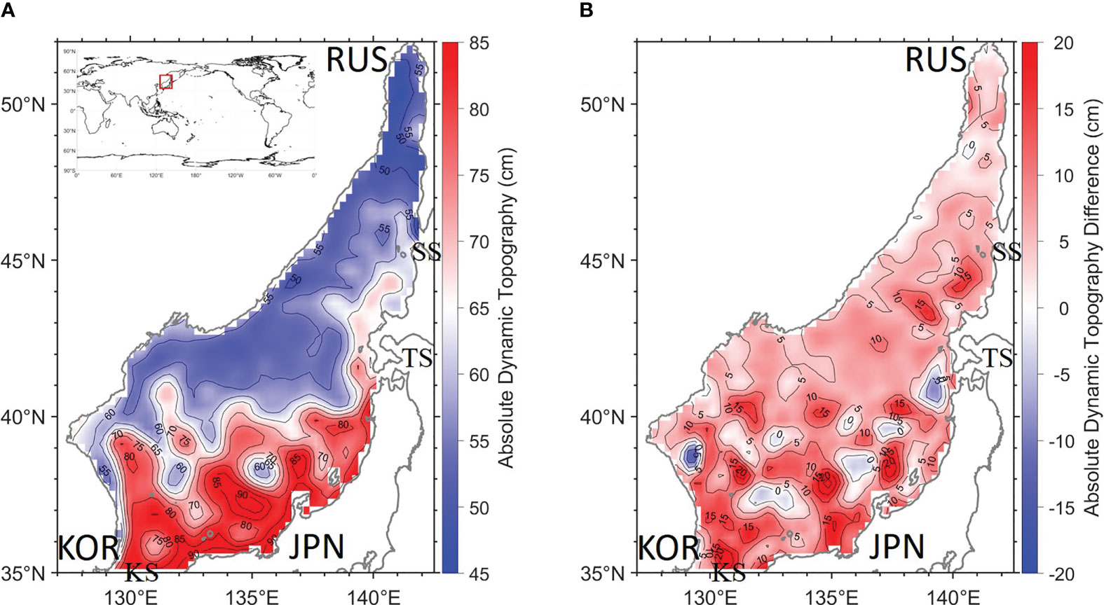
Figure 1 (A) Monthly mean sea level (MSL) in absolute dynamic topography (ADT) () in the East Sea (ES) in July 2021 and (B) sea level change (SLC) in ADT () from July 1 (00:00 UTC) to August 1 (00:00 UTC) in 2021 (ADT difference between 00:00 UTC August 1 and 00:00 UTC July 1 in 2021). The iso-ADT interval is 5 cm, and coastlines are drawn in gray. KOR, RUS, and JPN indicate Korea, Russia, and Japan, respectively. KS, TS, and SS denote Korea, Tsugaru, and Soya Straits, respectively. The ES is represented by a red solid rectangle on the map (upper left in (A)).
There is a marked seasonal variation of SL in the ES, with high values observed in summer and fall and low values observed in winter and spring due to the steric effect of seawater, mass exchange among the atmosphere and the three straits, and atmospheric pressure differences; the average SL variation is 30.4 cm between summer and winter from 1993 to 2018 (Han et al., 2020a). Furthermore, SL has gradually increased in the ES for decades owing to climate change, with an average increase rate of 3.78 mm year-1 from 1993 to 2017 (Han et al., 2020b). In addition to these seasonal variations and decadal trends in SL, an extreme value of the monthly MSL (from ADT measures) was recorded in July 2021; the SL was found to be 65.09 cm, which was the highest compared with previous July measurements of SL from 1993 to 2021. We present in Figure 1A) the monthly mean of the ADT in July 2021 contoured in the ES with a 5-cm interval, as measured by satellites. The ADT was high, particularly in the southern part of the ES, where mesoscale eddies were formed, and the iso-ADT lines fluctuated considerably around the eddies (Figure 1A). We calculated the ADT difference between the last and first days of July to eliminate the effect of previous months (Figure 1B). We found that the increase in ADT was higher in the southern ES than in the northern ES. As shown in Figure 2, the monthly mean ADT, atmospheric temperature (AT) at 2 m above the sea surface, and SST are compared in July of each year from 1993 to 2021. The ADT, AT, and SST reached their highest values in July 2021 (65.09 cm, 23.04°C, and 22.00°C, respectively). Thus, the highest recorded SL in July 2021 could be attributed to extreme values of heat flux from the atmosphere into the ocean and seawater temperature, as well as the rising SL trend due to global warming. In this study, we focused on the July ADT in 2021, as well as corresponding measures of ADT over the 29 years, and examined the factors that contributed to this unusually large increase.
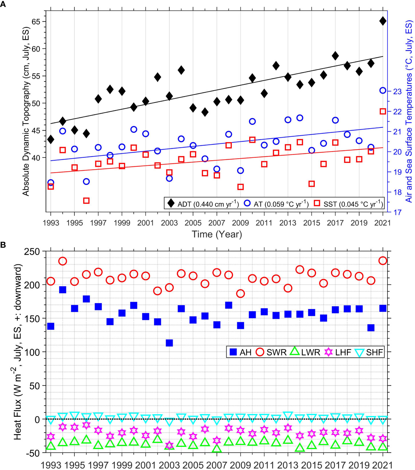
Figure 2 (A) July MSL in ADT (, m, black filled diamond, left y-axis), air temperature (°C, at 2 m above the sea surface, blue open circle, right y-axis), and sea surface temperature (°C, at 0 m, red open square, right y-axis) from 1993 to 2021. The solid lines represent their linear trends. (B) July atmospheric net heat flux (AH, W m-2, positive means downward, blue-filled square), July shortwave radiation flux (SWR, W m-2, positive means downward, red open circle), July longwave radiation flux (LWR, W m-2, positive means downward, green open upward triangle), July latent heat flux (LHF, W m-2, positive means downward, magenta hexagon), and July sensible heat flux (SHF, W m-2, positive means downward, cyan open downward triangle) from 1993 to 2021.
The authors of previous studies (Pinardi et al., 2014; Han et al., 2020a; Han et al., 2020b) have established that increasing the heat and mass in a semi-enclosed sea, such as the ES, raises the SL. For example, SL increases and decreases with the rise and fall in AT and SST if the effects of mass and atmospheric pressure on SL are negligible. The temperature of the water that flows into the ES through the KS is higher than that of the water in the ES, generally, and the water that flows through the TS/SS, because the water in the KS originates from lower latitudes. If we assume that the mass transport flows into and out of the ES are identical (although this is not actually the case, the seawater entering from the KS is warmer than seawater exiting from the TS/SS. Therefore, the temperature difference between the KS and TS/SS can increase the temperature of the ES, which is then released from the ocean into the atmosphere via the sea surface. If we assume that the heat released into the atmosphere is constant over time (although this is not the case, as shown in Figure 2B), the seawater heat difference anomaly between the KS and TS/SS can contribute to the SL variation in the ES due to thermal expansion and contraction of the upper layer of the seawater. In contrast, if the difference in heat transport between the KS and TS/SS is assumed to be identical (although this is not actually the case, the SL in the ES would increase or decrease in response to changes in the surface net incoming heat flux, reflected in the corresponding expansion and contraction of the upper layer of water in the ES.
Another consideration is the changes in mass transport. As shown in Figure 1, a branch of the Kuroshio Current flows into the ES via the KS, and seawater flows out via the two narrower straits, TS and SS, because the mass transport through the Tatarsky Strait and other gaps between the ES and surrounding waters can be negligible (Hirose et al., 1996; Lyu et al., 2002). Therefore, the difference in mass transport among these straits can affect the SL of the ES. Furthermore, the length of time that seawater stays in the ES after entering through the KS could be prolonged when the pathways of the main currents are changed by the formation of mesoscale eddies, which leads to an increased residence time of these currents in the ES. Therefore, the extended residence time of the incoming water could be one of the reasons the SL is raised when the incoming mass transport through the KS exceeds the outgoing mass transport through the TS/SS. In the present study, we examined the abovementioned factors to determine what led to the extreme SL values in July 2021.
The CMEMS dataset provides ADT of a 0.25° horizontal grid from all satellite altimeter missions, in two formats: near-real time and reprocessed data. We analyzed the reprocessed level 4 daily ADT (CMEMS_portal, 2023) in the ES in July over 29 years (1993 to 2021) to calculate the monthly MSL (for example, July MSL is the mean of daily ADT values from July 1 to July 31) and monthly sea level change (SLC; for example, July SLC is calculated by subtracting ADT at 00:00 UTC on July 1 from ADT at 00:00 UTC on August 1) as follows:
where , , and ND indicate the monthly MSL as reflected in ADT (m), daily ADT (m), and number of days in a month, respectively. The MSL of the ES was calculated using area weighting because the longitudinal angular distance decreases as the latitude increases.
where represents the monthly SLC as reflected in ADT within a month (m). and represent the daily ADT values on the first (e.g., 00:00 UTC on July 1) and last (e.g., 00:00 UTC on August 1) days of the month (m). represents the monthly SLC in Atmospheric sea surface net Heat flux (AH, m) in Eq. (3). represents the monthly SLC in Oceanic lateral Heat transport divergence (OH, m) among the KS, TS, and SS in Eq. (4). represents the monthly SLC in oceanic Mass transport divergence including other Errors (ME) in Eq. (5). Therefore, SLCADT was obtained by calculating the difference between the daily ADT values of the last and first days of the month (). This difference is equal to the sum of the monthly SLC value attributed to atmospheric heat, oceanic heat, and oceanic mass including other errors (. To calculate a mixed layer depth at which the water temperature first drops by 0.02°C below the SST (Cummings and Smedstad, 2013), we analyzed the daily mean SST from the Optimum Interpolated Sea Surface Temperature dataset (OISST; ver. 2; obtained from the National Oceanic and Atmospheric Administration [NOAA] National Centers for Environmental Information [NCEI] (NCEI_OISST, 2023)), which consists of data in a horizontal 0.25° grid (Reynolds et al., 2007), and the monthly mean water potential temperature, salinity, and water potential density from HYCOM global reanalysis and analysis of a horizontal 0.08° grid (GOFS 3.1 GLBb0.08, HYCOM_GOFS_3.1_Analysis, 2023; HYCOM_GOFS_3.1_Reanalysis, 2023). We examined the monthly mean ERA5 data (ERA5_monthly_averaged, 2023) of a horizontal 0.25° grid published by the European Centre for Medium-Range Weather Forecasts (ECMWF). These ERA5 data include sea surface shortwave radiation flux (SWR), longwave radiation flux (LWR), latent heat flux (LHF), sensible heat flux (SHF), and AT at 2 m above the sea surface, which can affect the SL of the ES (Hersbach et al., 2020). The thermal expansion of the SLC ([m]) caused by atmospheric sea surface net heat flux ( [W m-2]; sum of SWR, LWR, LHF, and SHF from the atmosphere to ocean) was calculated as follows:
where , , , and represent SWR, LWR, LHF, and SHF, respectively, all reported in W m-2. , , , , and represent the sea surface horizontal area in the ES (~1012 m2), thermal expansion coefficient for seawater (°C-1), specific heat capacity for seawater (~4,000 J kg-1°C-1), water potential density (kg m-3) at the middle depth between the surface and mixed layer depth, and time (a month in seconds), respectively. , , , , , and represent longitude, the westernmost and easternmost points, latitude, and the southernmost and northernmost points (°), respectively. The in Eq. (3) is the sea surface integral of vertical contraction/expansion of the sea water caused by surface net heat flux from the atmosphere to ocean in the ES.
The monthly mean horizontal water velocity with water potential temperature, salinity, and water potential density from HYCOM global reanalysis and analysis of a horizontal 0.08° grid (GOFS 3.1 GLBb0.08, HYCOM_GOFS_3.1_Analysis, 2023; HYCOM_GOFS_3.1_Reanalysis, 2023) were also used to calculate , as shown in Eq. (4):
where , , , and represent the OH among the KS, TS, and SS (J s-1); meridional velocity in the KS (m s-1); and zonal velocities in the TS and SS (m s-1), respectively. , , , , , , and represent water potential temperatures in the KS, TS, and SS (°C), reference temperature which we take to be 0°C, and thermal expansion coefficients in the KS, TS, and SS (°C-1), respectively. , , , and represent depths in the KS, TS, and SS (m) and depth (m), respectively. The first term of the last right-hand side of Eq. (4) is the SLC caused by the vertical sectional integral of incoming heat transport that passes through the KS into the ES, and the second and third terms are the SLCs caused by the vertical sectional integrals of outgoing heat transports that pass through the TS and SS out of the ES, respectively. is calculated as shown in Eq. (5)
The in Eq. (5) is the SLC attributed to oceanic mass transport divergence including other errors and is computed by subtracting the SLCs attributed to the atmospheric and oceanic net heat fluxes from the SLC in ADT.
As described in Section 2.1.2, one of the main mechanisms that may contribute to SL elevation in the ES is thermal expansion caused by excessive incoming heat into the water, as illustrated in Figure 2A), which shows the SST and AT at 2 m above the sea surface compared with the calculated using Eq. (1) in July for 29 years. SST and AT were both significantly higher in 2021 (23.04°C and 22.00°C, respectively) than in the previous years. In contrast, the wind speed in July 2021 was less than 2 m s-1, which was lower than the average of the previous years (not shown). The results in Figure 2A) (SST and AT) indicate that thermal expansion may be a major cause of the high SL in July 2021, whereas the low wind speed could indicate the possibility of high atmospheric pressure and/or no strong atmospheric pressure gradients in the ES during the corresponding month.
To investigate this possibility, the monthly mean data of the AH, SWR, LWR, LHF, and SHF were estimated using ERA5; the July data are compared in Figure 2B). In the 29-year dataset, SWR (235.62 W m-2, red open circle) was at its highest in July 2021. In contrast, no discernible anomalies were observed in the AH, LWR, LHF, and SHF values in 2021. The significant SWR in 2021 indicates that incoming solar radiation into seawater increased in the corresponding month, most likely due to clear weather with little cloud cover, resulting in higher SST and AT, as shown in Figure 2A). This is an unusual occurrence considering that July is typically the rainy season on the Korean Peninsula.
We compared the July using Eq. (1) with the in May, June, and August, as shown in Figure 3A). The monthly MSL trends in May, June, July, and August were 0.40, 0.43, 0.44, and 0.49 cm yr-1, respectively (Figure 3A). The MSLs in 2021 (June, July, and August) are the maxima from 1993 to 2021, except for the MSL in May, because the have increasing trends (global warming). During the 29-year time period, the highest in July (2021) may have been caused by the highest in June (see Figure 3A). We calculated the SLC for each month () using Eq. (2), as shown in Figure 3B), to investigate the net monthly SLC without the influence of previous months. The in 2021 were as follows (in cm): −2.60 (February), −1.42 (March), 5.13 (April), −1.10 (May), 8.83 (June), 7.18 (July), and −5.94 (August) (Figure 3B). The in June (8.83 cm) and July (7.18 cm) in 2021 were the highest SLC in June and fifth highest in July, respectively, for the 29-year period (1993–2021). Thus, the highest in July 2021 (Figure 2A) is due to the in June and July 2021 (sum of red and green bars in 2021 in Figure 3B). The in July in the ES is a cumulative consequence of the water volume, both during the previous month and in July itself; therefore, the of the previous month can affect the of the next month in a semi-enclosed basin such as the ES. Additionally, the highest in August 1994 excluding the trend (the height from the dotted blue line to blue open square in Figure 3A) is the sum of the in June, July, and August of that year (sum of red, green, and blue bars in 1994 in Figure 3B) because in May is sufficiently negative to cancel out the positive in March and April.

Figure 3 (A) Monthly MSL in ADT ( ) in May (black open diamond), June (red open circle), July (green triangle), and August (blue square) from 1993 to 2021. The dashed lines represent their trends. (B) SLC in ADT ( ) in February (yellow), March (magenta), April (cyan), May (black), June (red), July (green), and August (blue) from 1993 to 2021.
There are two sources of SLC in the ES: the atmosphere and the ocean. The sources of heat and mass from the atmosphere are the AH and precipitation minus evaporation, respectively. If we ignore the effects of precipitation minus evaporation on SL in the ES, we can compute the atmospheric effect on SL () based on the AH using Eq. (3). Based on HYCOM and ERA5 reanalysis data, the contribution of AH to SL in 2021 can be determined by the thermal expansion of seawater from the surface to the mixed layer depth in May (Figure 4B), June (Figure 4F), July (Figure 4J), and August (Figure 4N). The can be averaged in the ES in May, June, July, and August 2021 (blue open square in Figure 5) and can be extended from 1994 to 2021 as July to compare them only in July during the observational period in Figure 6. Regardless of the values in June (2.35 cm) and July (2.87 cm) in 2021 in Figures 4F, J), its direct contribution to the in July 2021 was estimated to be less than 3 cm. Therefore, the thermal expansion caused by the increased heat transfer from the atmosphere to the ocean may not be a controlling factor for the extreme in the ES in July 2021 as well as for the from 1993 to 2021; thus, additional factors need to be considered. From 1994 to 2021, the mean ± standard deviations of the and were 4.57 ± 2.79 and 2.48 ± 0.27 cm, respectively, and the ratio of to was 54.32 ± 9.84% (Figure 6).
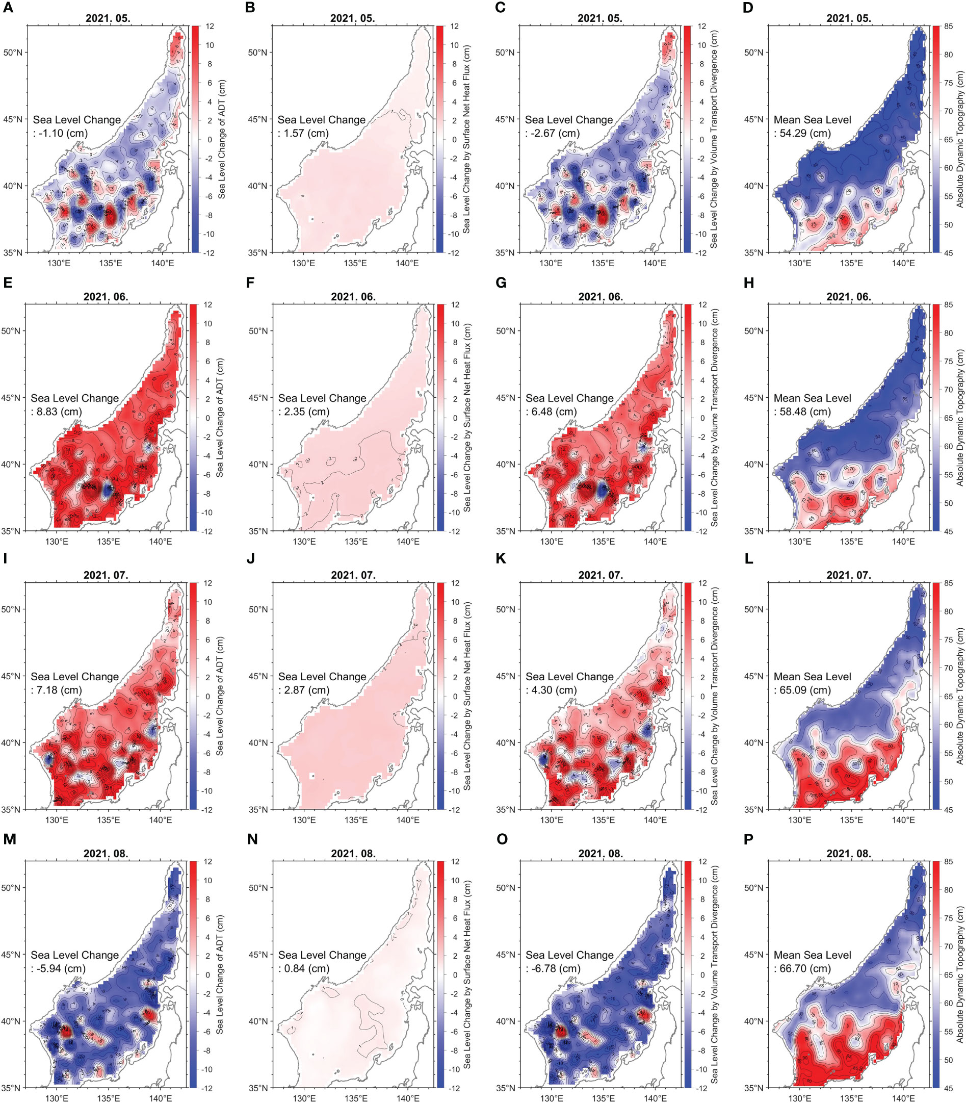
Figure 4 Horizontal SLC in ADT () in (A) May, (E) June, (I) July, and (M) August in 2021. Horizontal SLC in AH () in (B) May, (F) June, (J) July, and (N) August 2021. SLC in ADT minus SLC in AH () in (C) May, (G) June, (K) July, and (O) August 2021. MSL in ADT () in (D) May, (H) June, (L) July, and (P) August 2021.
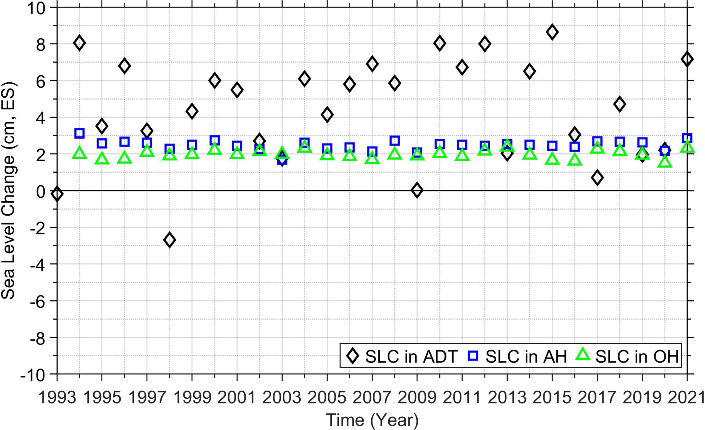
Figure 5 SLC in ADT (, black open diamond), AH (, blue open square), and OH (, green open triangle) in July from 1993 to 2021.
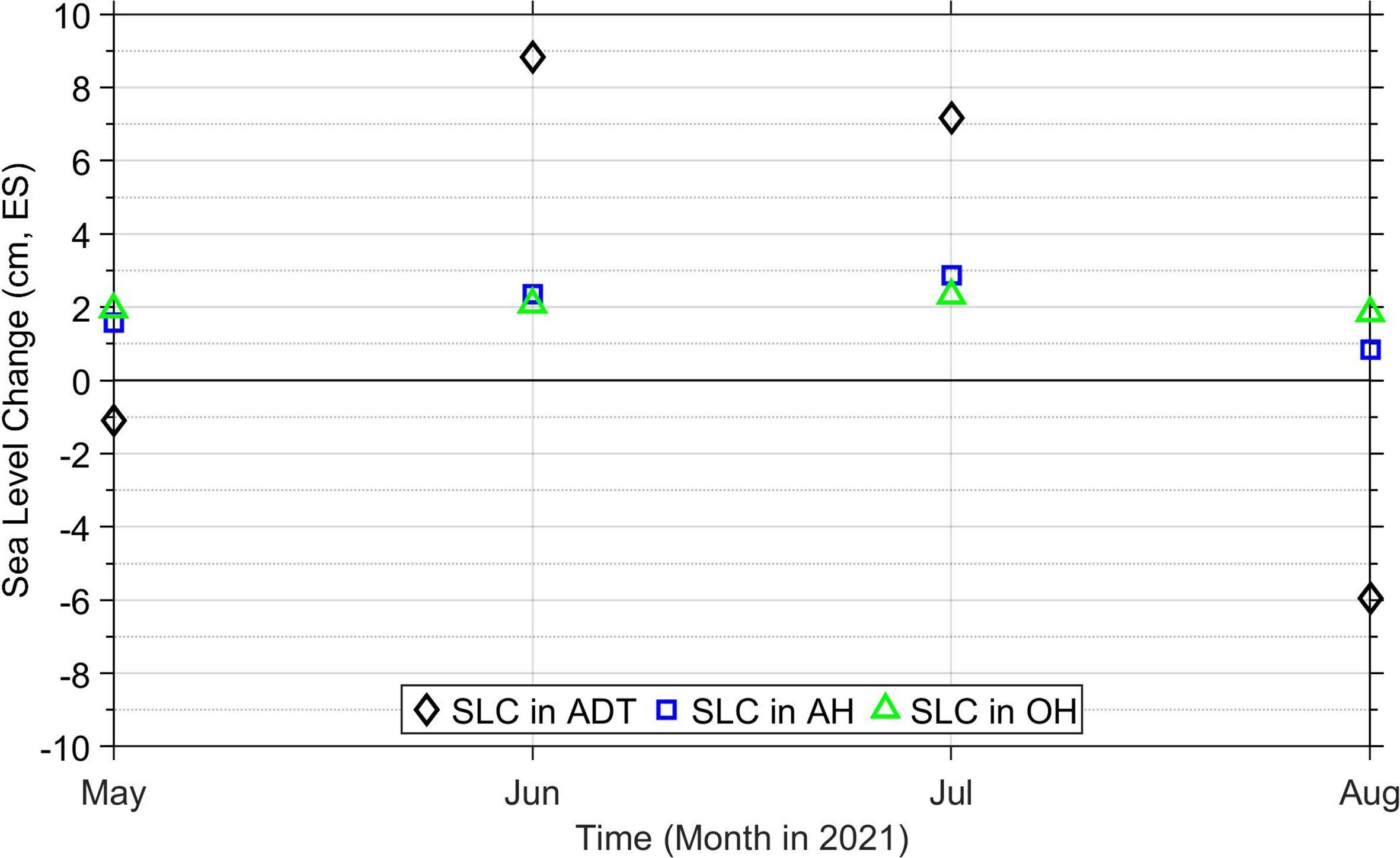
Figure 6 SLC in ADT (, black open diamond), AH (, blue open square), and OH (, green open triangle) in May, June, July, and August 2021.
We present in Figure 4 the horizontal distributions of the monthly (May, June, July, and August) values of (Eq. (2)), (Eq. (3)), (, Eqs. (4) and (5)), and from satellite data (Eq. (1)). In contrast to the flat horizontal , the resembles the total . Values for were estimated to be 6.48 cm (June) and 4.30 cm (July) in 2021, which were 2.8 (6.48 cm/2.35 cm) and 1.5 (4.30 cm/2.87 cm) times larger than the in June and July, respectively.
In addition to these results, we calculated the during May, June, July, and August among the KS, TS, and SS using the HYCOM reanalysis and analysis data (Figure 5). Accordingly, in June and July 2021, the values of were 2.08 and 2.32 cm (green open triangle, Figure 5), respectively. Thus, there was more heat from incoming seawater in July than in June. We found that the highest , which occurred in July 2021 (65.09 cm), was caused not only by in July (2.32 cm) but also by in June (2.08 cm), because seawater can accumulate in a semi-enclosed sea over time. Furthermore, the data shown in Figure 5 were only estimated from May to August, given that the highest (July 2021) was primarily controlled by atmospheric and oceanic net heat fluxes (and ) in June and July.
In the 29-year data period, the highest July occurred in 2021 (black-filled diamond in Figure 2A) due to the trend (0.44 cm year-1, Figure 2A), the high in June (8.83 cm; Figure 4E, black open diamond in Figure 5), and the high (2.35 and 2.87 cm in June and July; blue open square in Figure 5) and (2.08 and 2.32 cm in June and July; green open triangle in Figure 5) in June and July 2021. Thus, the highest July , in 2021, was the result of the in the previous month (June), along with the values affected by oceanic and atmospheric effects. From 1994 to 2021, the mean ± standard deviation of the was 1.97 ± 0.22 cm, and the relative contribution of to was 43.06 ± 8.02% (Figure 6). The standard deviation of is 2.70 cm and 96.73% (2.70 cm/2.79 cm) of that of from 1994 to 2021, which means that the variance of ocean mass transport divergence including other errors is large and similar to that of .
In this study, we have investigated several factors that possibly contributed to the extreme (65.09 cm) in July 2021, as well as the atmospheric and oceanic factors affecting July , in general, over the 29 years of the dataset. The in July 2021, as estimated using satellite observations, was approximately 7.18 cm, which was the fifth highest among July observations over 29 years (Figure 3). The in June was approximately 8.83 cm, which was the highest June over the 29-year period (Figure 3) and affected the in July because the latter included the former. Although both SST and AT increased significantly—likely due to mostly clear skies, which caused the unusually high SWR level in the corresponding month—the was estimated to be 40.0% of in July 2021, which is less than the average value (54.32%) over the 29 years. In July, the atmospheric source of sea level change () was the highest among the sources of sea level change (, , and ). However, the sources from others (and ) accounted for approximately 60.0% of in July 2021.
One of the major factors that contributed to the MSL peak in July 2021 may have been the increase in the mass transport divergence including errors (, 4.40 cm) in June in the ES. Owing to the unusual atmospheric phenomena of high MSL atmospheric pressure patterns in the northwestern Pacific, the Ekman transport into the ES caused by wind stress anomaly and its curl distribution around the ES may have contributed to an increase in the seawater that enters the ES via the KS but decrease in the seawater that exits the ES through the TS and SS (not shown), resulting in an increase in the seawater and ADT in the ES. Additional evidence of this process can be found in the distribution shown in Figure 1A, where several mesoscale eddies developed in the southern part of the ES and the iso-ADT lines showed strong meandering around the eddies. Enhancement of the meandering of the currents and formation of more eddies could make the seawater remain in the ES, with a longer residence time, resulting in increased , and .
In calculating , the right-hand side of Eq. (5), , was used instead of using reanalysis data, namely, HYCOM, because of the uncertainty of the reanalysis data. In the case of HYCOM, for example, the accuracy of mass transport divergence calculation might not be satisfactory in the ES, because the horizontal resolution of 0.08° could be too coarse to be applied within this relatively small-sized marginal sea, although the resolution is sufficiently fine to be applied to the global ocean. Another possibility for the uncertainty might be the regridding. The HYCOM output was interpolated in the new grids that were different from the original modeling grids in the ES, which might have increased the error. In addition, the velocity and density data were assimilated in HYCOM. Therefore, small changes in these data could have a significant impact, especially in calculating the mass transport divergence, compared with the other parameter (heat transport divergence) evaluated in this study. Owing to these reasons, the final output did not satisfy the mass or volume balance within the ES as the mean ± standard deviation of the based on ocean mass transport divergence among straits calculated from HYCOM was 5.56 ± 5.36 cm, which is larger than that of the (4.57 ± 2.79 cm) over the 29 years. Thus, we have used in Eq. (5), not directly calculation from HYCOM. In addition, could have errors from satellite ADT data which were interpolated spatially using tracked satellite data, from sea surface heat flux data of ERA 5 reanalysis data, and from ocean heat transport of HYCOM reanalysis data.
The increase in the input mass of seawater through KS might induce an additional increase for the in the ES if precipitation minus evaporation plus runoff is negligible. Because the KS is located at the southwestern end of the ES, the seawater that enters into the ES is a part of the branch of the Kuroshio Current, Tsushima Warm Current, and had a higher temperature than that of the seawater in the ES. Therefore, the increase in mass transport in the KS is followed by an increase in heat and mass into the ES. Alternatively, the decrease in output mass transport through TS and SS might induce heat and mass increases in the ES since the heat and mass could stay longer in the ES. This impact of heat transport was significant, as the estimated between the KS and TS/SS was 2.32 cm, accounting for approximately 32.3% of the in July 2021. Also, the increase in was 2.87 cm, accounting for approximately 40.0% of in July 2021 (Table 1). Therefore, our findings suggest that atmospheric and oceanic heat fluxes may be the two major mechanisms underlying SL variation in the ES. However, the factors that influence ocean mass transport remain unclear. The unusually high and low atmospheric pressure anomalies in the ES and East China Sea, respectively, in July 2021 may be one of the controlling factors for the ; however, this is not always the case in other years. In the ES, rainy season usually begins in late June or early July, and generally, there is low atmospheric pressure. Therefore, the existence of high atmospheric pressure in July 2021 was unusual, and future research may be required to investigate the relationship between atmospheric pressure, rainfall, and the SL pattern in the ES during this season.
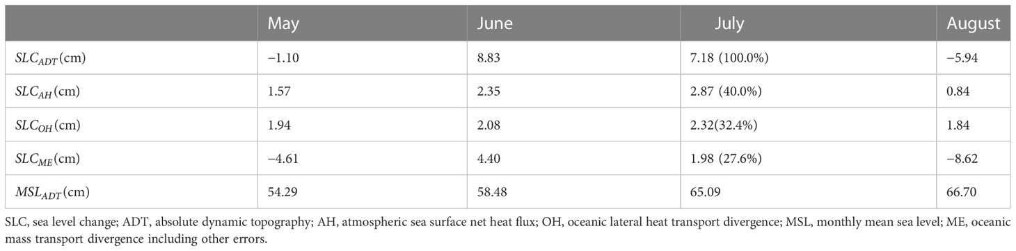
Table 1 SLCs in ADT (), AH (), OH (), and ME (), and MSL in ADT () in May, June, July, and August 2021.
Climate indices, such as the Arctic Oscillation Index (AOI, Rigor et al., 2002), East Asian Summer Monsoon Index (EASMI, Zhao et al., 2015; Huang and Zhao, 2019), North Pacific Gyre Oscillation (NPGO, Di Lorenzo et al., 2008), North Pacific Index (NPI, Trenberth and Hurrell, 1994)), Oceanic Niño Index (ONI, Hafez, 2016), and Pacific Decadal Oscillation (PDO, Di Lorenzo et al., 2008), in July from 1994 to 2021 were used to compare the variabilities in , , and Only and EASMI, and EASMI, and and PDO were significantly correlated (correlation coefficients (R): −0.47 (p-value = 0.01), −0.52 (p-value = 0.00), and −0.37 (p-value = 0.05) (Figures 7 and 8). The first and second correlation coefficients indicate that the effects of thermosteric sea level fluctuations from the atmosphere and surrounding seas and ocean into the ES ( and ) are related to the East Asian summer monsoon (EASM). The EASMI was calculated with a mean zonal wind at 200 hPa as it is related to horizontal vorticity and vertical motion of the air (Zhao et al., 2015). These air motions are related to precipitation, especially the mei-yu–changma–baiu rainfall in July, which could release condensational heat in the atmosphere (Zhao et al., 2015), and to the subtropical ocean and north Pacific SST (Lee et al., 2008). Thus, thermosteric SLC caused by the atmospheric and oceanic heat ( and ) related to the EASM changes with EASMI significantly as showed in correlation coefficients above. In addition, the thermosteric SLC caused by heat transport divergence from the surrounding seas and ocean into the ES () is related to the PDO negatively, which means the sea level rises when the PDO is negative. The SST anomaly in the western Pacific is positive when the PDO is negative, indicating that there is higher heat in the seas and ocean around the ES than that when the PDO is not negative. Consequently, When the PDO is negative, the SST in the western Pacific rises above average and the Kuroshio weakens, allowing the strong Tsushima Warm Current to enter the ES to a greater degree. As a result, the thermosteric SLC () in the ES increases when the PDO is negative (Gordon and Giulivi, 2004; Han and Huang, 2008; Andres et al., 2009).
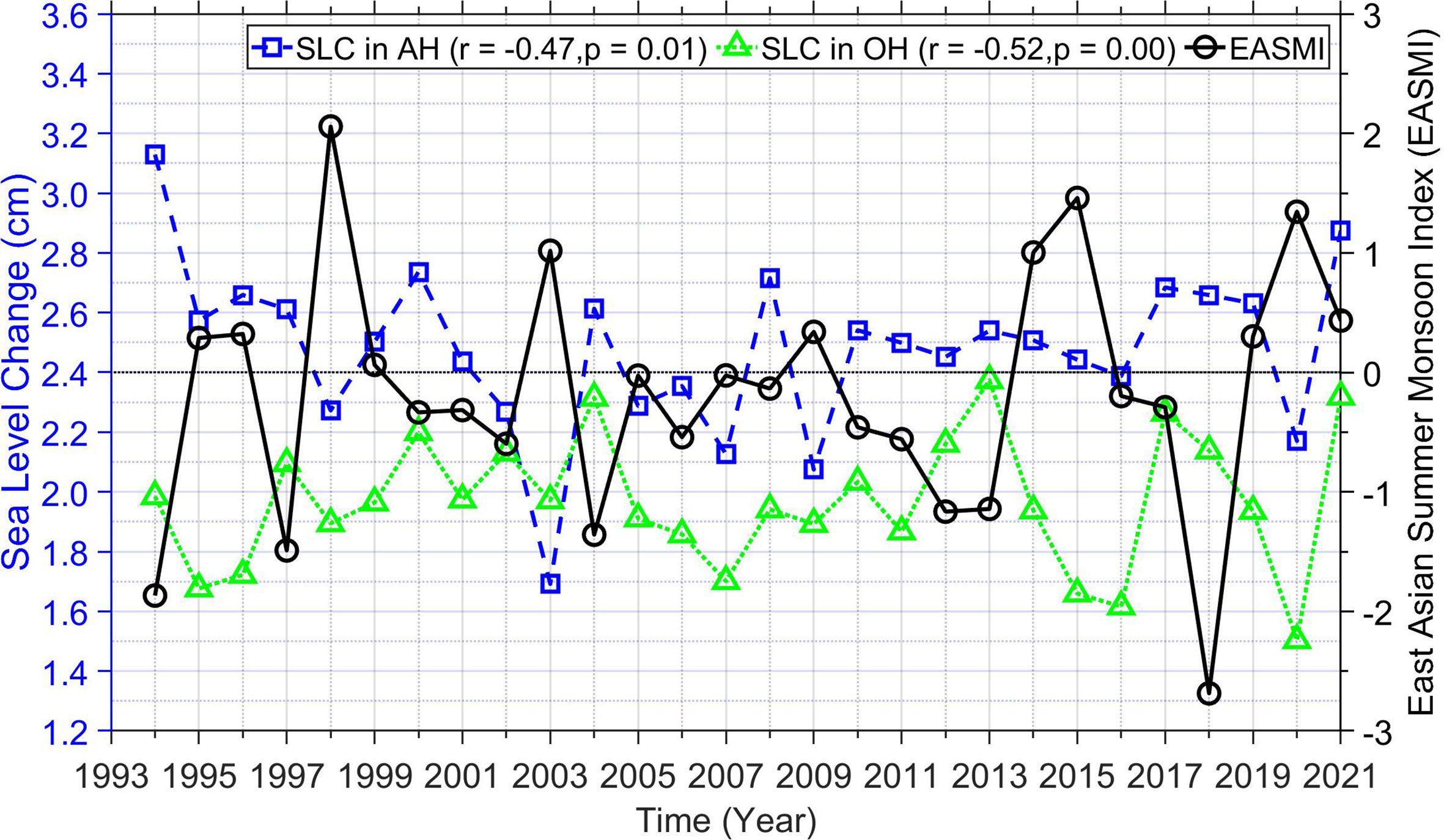
Figure 7 SLC in AH (, blue open square, left Y-axis) and OH (, green open triangle, left Y-axis), and the East Asian Summer Monsoon Index (EASMI; black open circle, right Y-axis) in July from 1994 to 2021. The correlations between and EASMI and between and EASMI are −0.47 (p-value = 0.01) and −0.52 (p-value = 0.00), respectively.

Figure 8 SLC in OH (, green open triangle, left Y-axis) and Pacific Decadal Oscillation (PDO; black open square, right Y-axis) in July from 1994 to 2021. The correlation coefficient between and PDO is −0.37 (p-value = 0.05).
The causes of SL variation in a semi-enclosed sea are more complex than those in an open ocean. The thermosteric effect of seawater caused by the ocean and atmosphere is closely related to in a semi-enclosed sea. The values in Table 1 show that heat contributed 72.4% in 2021. From 1994 to 2021, the percentage of caused by heat was 97.4% (Figure 9). The mean ± standard deviation of the was 0.12 ± 2.70 cm, and the relative contribution of to was 2.62 ± 96.73%, which shows a severe undulation of the ocean mass transport divergence in the ES including other errors. Seawater can accumulate and remain in a semi-enclosed sea over time; thus, previous due to mass and heat (e.g., 1 month before) can influence future SLs (e.g., 1 month later). Therefore, to understand the SL and its warming trend, we must take the previous mass and heat fluxes into consideration. Furthermore, the SL variation in the ES is related to the EASM and PDO, indicating the influence of regional and global climate change at the local sea level in a warming climate. In this study, we proposed several methods for deconstructing the causes of in a semi-enclosed sea during a period of rapid SL rise. Our results provide a foundation for future SLC research in this area; for example, to understand SLC well, precise mass calculation from the atmosphere, the land, and the ocean to the ES should be investigated, as well as error computation of heat from the atmosphere and the ocean to the ES in the near future.
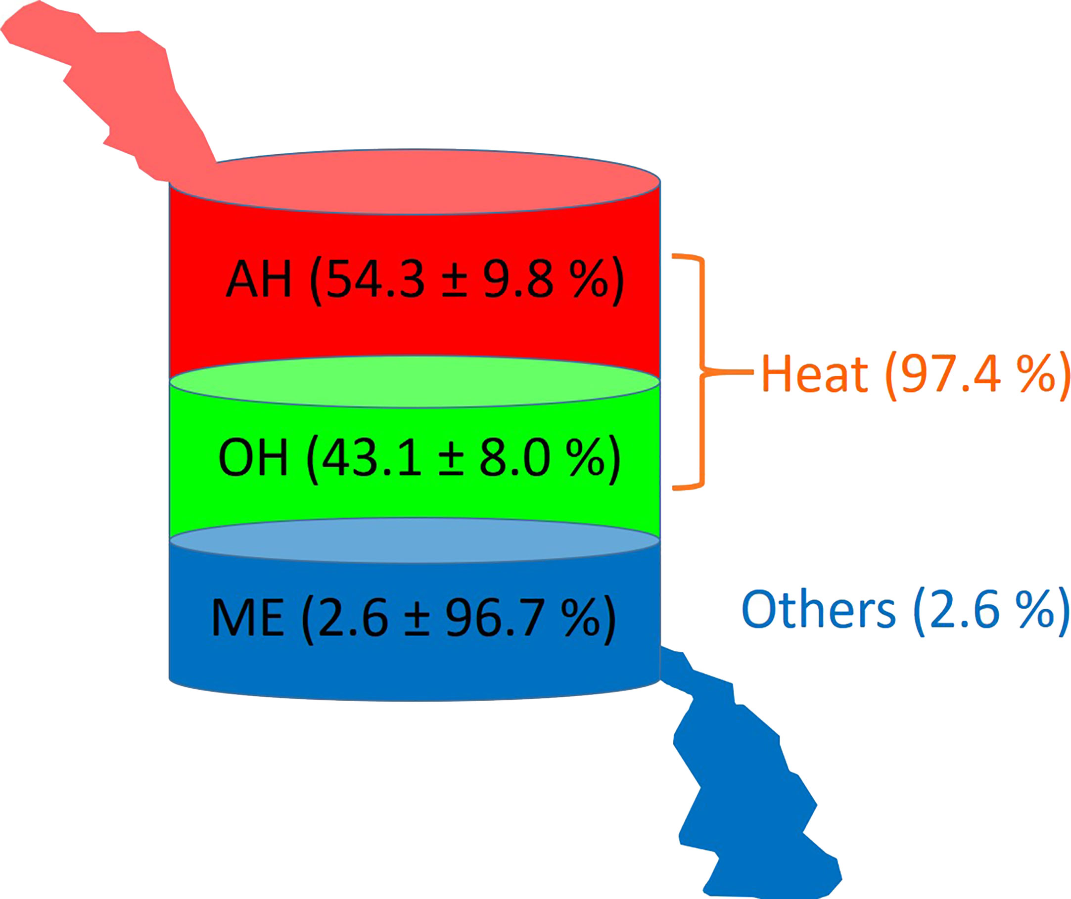
Figure 9 Schematic of the sources of SLC in July, from 1994 to 2021 in the ES. Relative contribution of atmospheric and oceanic heat was 54.3% and 43.1%, respectively, and heat and other sources (mass + errors) accounted for 97.4% and 2.6%, respectively.
The original contributions presented in the study are included in the article/Supplementary Material. Further inquiries can be directed to the corresponding author.
MH conceived of the study and performed all data analyses. MH, YC, and JY contributed to the writing of the manuscript as well as the conceptualization and interpretation of the results.
This research was supported by Korea Institute of Marine Science & Technology Promotion (KIMST) funded by the Ministry of Oceans and Fisheries [(20220431, Development of Simulation Technology for Maritime Spatial Policy), (20210607, Establishment of the Ocean Research Station in the Jurisdiction Zone and Convergence Research), and (20220033, Assessment and Long-Term Projections of Ocean Climate Change)].
Satellite altimetry data (SSALTO/DUACS altimeter products) produced and distributed by the CMEMS (http://www.marine.copernicus.eu), OISST data from the NOAA Physical Science Laboratory (https://psl.noaa.gov/data/gridded/data.noaa.oisst.v2.highres.html), and surface heat flux data from the ECMWF Reanalysis v5 (http://www.ecmwf.int/) were used in this study. The National Ocean Partnership Program and Office of Naval Research have provided funding for the development of HYCOM. Data assimilation products using HYCOM are funded by the U.S. Navy. Computer time was made available by the DoD High-Performance Computing Modernization Program. The output is publicly available at https://hycom.org. We thank H-. W. Kang and Y. S. Kim for their helpful advice and suggestions in the project design and data analysis.
The authors declare that the research was conducted in the absence of any commercial or financial relationships that could be construed as a potential conflict of interest.
All claims expressed in this article are solely those of the authors and do not necessarily represent those of their affiliated organizations, or those of the publisher, the editors and the reviewers. Any product that may be evaluated in this article, or claim that may be made by its manufacturer, is not guaranteed or endorsed by the publisher.
Andres M., Park J. H., Wimbush M., Zhu X. H., Nakamura H., Kim K., et al. (2009). Manifestation of the pacific decadal oscillation in the kuroshio. Geophysical Res. Lett. 36 (16). doi: 10.1029/2009GL039216
Calafat F., Chambers D. (2013). Quantifying recent acceleration in sea level unrelated to internal climate variability. Geophysical Res. Lett. 40 (14), 3661–3666. doi: 10.1002/grl.50731
Casey K. S., Adamec D. (2002). Sea Surface temperature and sea surface height variability in the north pacific ocean from 1993 to 1999. J. Geophysical Research: Oceans 107 (C8), 14–11-14-12. doi: 10.1029/2001JC001060
Cazenave A., Palanisamy H., Ablain M. (2018). Contemporary sea level changes from satellite altimetry: what have we learned? what are the new challenges? Adv. Space Res. 62 (7), 1639–1653. doi: 10.1016/j.asr.2018.07.017
Church J. A., White N. J. (2011). Sea-Level rise from the late 19th to the early 21st century. Surveys geophysics 32 (4), 585–602. doi: 10.1007/s10712-011-9119-1
CMEMS_portal (2023) Cmems_obs-sl_glo_phy-ssh_my_allsat-l4-duacs-0.25deg_P1D. Available at: ftp://my.cmems-du.eu/Core/SEALEVEL_GLO_PHY_L4_MY_008_047/cmems_obs-sl_glo_phy-ssh_my_allsat-l4-duacs-0.25deg_P1D (Accessed 28 February, 2023).
Cummings J. A., Smedstad O. M. (2013). “Variational data assimilation for the global ocean,” in Data assimilation for atmospheric, oceanic and hydrologic applications, vol. II. (Springer), 303–343.
Dangendorf S., Mudersbach C., Wahl T., Jensen J. (2013). Characteristics of intra-, inter-annual and decadal sea-level variability and the role of meteorological forcing: the long record of cuxhaven. Ocean Dynamics 63 (2), 209–224. doi: 10.1007/s10236-013-0598-0
Di Lorenzo E., Schneider N., Cobb K. M., Franks P., Chhak K., Miller A. J., et al. (2008). North pacific gyre oscillation links ocean climate and ecosystem change. Geophysical Res. Lett. 35 (8). doi: 10.1029/2007GL032838
Ducet N., Le Traon P.-Y., Reverdin G. (2000). Global high-resolution mapping of ocean circulation from TOPEX/Poseidon and ERS-1 and-2. J. Geophysical Research: Oceans 105 (C8), 19477–19498. doi: 10.1029/2000JC900063
ERA5_monthly_averaged (2023) ERA5 monthly averaged data on single levels from 1959 to present. Available at: https://cds.climate.copernicus.eu/cdsapp#!/dataset/reanalysis-era5-single-levels-monthly-means?tab=form (Accessed 28 February, 2023).
Fasullo J. T., Gent P. R. (2017). On the relationship between regional ocean heat content and sea surface height. J. Climate 30 (22), 9195–9211. doi: 10.1175/JCLI-D-16-0920.1
González-Haro C., Isern-Fontanet J., Tandeo P., Garello R. (2020). Ocean surface currents reconstruction: spectral characterization of the transfer function between SST and SSH. J. Geophysical Research: Oceans 125 (10), e2019JC015958. doi: 10.1029/2019JC015958
Gordon A. L., Giulivi C. F. (2004). Pacific decadal oscillation and sea level in the Japan/East Sea. Deep Sea Res. Part I: Oceanographic Res. Papers 51 (5), 653–663. doi: 10.1016/j.dsr.2004.02.005
Hafez Y. (2016). Study on the relationship between the oceanic nino index and surface air temperature and precipitation rate over the kingdom of Saudi Arabia. J. Geosci. Environ. Prot. 4 (05), 146. doi: 10.4236/gep.2016.45015
Haigh I. D., Wahl T., Rohling E. J., Price R. M., Pattiaratchi C. B., Calafat F. M., et al. (2014). Timescales for detecting a significant acceleration in sea level rise. Nat. Commun. 5 (1), 1–11. doi: 10.1038/ncomms4635
Han M., Cho Y.-K., Kang H.-W., Nam S., Byun D.-S., Jeong K.-Y., et al. (2020a). Impacts of atmospheric pressure on the annual maximum of monthly Sea-levels in the northeast Asian marginal seas. J. Mar. Sci. Eng. 8 (6), 425. doi: 10.3390/jmse8060425
Han G., Huang W. (2008). Pacific decadal oscillation and sea level variability in the bohai, yellow, and East China seas. J. Phys. Oceanography 38 (12), 2772–2783. doi: 10.1175/2008JPO3885.1
Han M., Nam S., Cho Y.-K., Kang H.-W., Jeong K.-Y., Lee E. (2020b). Interannual variability of winter Sea levels induced by local wind stress in the northeast Asian marginal seas: 1993–2017. J. Mar. Sci. Eng. 8 (10), 774. doi: 10.3390/jmse8100774
Hersbach H., Bell B., Berrisford P., Hirahara S., Horányi A., Muñoz-Sabater J., et al. (2020). The ERA5 global reanalysis. Q. J. R. Meteorological Soc. 146 (730), 1999–2049. doi: 10.1002/qj.3803
Hirose N., Kim C.-H., Yoon J.-H. (1996). Heat budget in the Japan Sea. J. Oceanography 52, 553–574. doi: 10.1007/BF02238321
Horwath M., Gutknecht B. D., Cazenave A., Palanisamy H. K., Marti F., Paul F., et al. (2022). Global sea-level budget and ocean-mass budget, with a focus on advanced data products and uncertainty characterisation. Earth System Sci. Data 14 (2), 411–447. doi: 10.5194/essd-14-411-2022
Huang G., Zhao G. (2019). The East Asian summer monsoon index, (1851–2021). Natl. Tibetan Plateau/Third Pole Environ. Data Center. doi: 10.11888/Meteoro.tpdc.270323
HYCOM_GOFS_3.1_Analysis (2023) HYCOM GOFS 3.1 analysis. Available at: ftp://ftp.hycom.org/datasets/GLBb0.08/expt_93.0/data/meanstd/ (Accessed 28 February, 2023).
HYCOM_GOFS_3.1_Reanalysis (2023) HYCOM GOFS 3.1 reanalysis. Available at: ftp://ftp.hycom.org/datasets/GLBb0.08/expt_53.X/data/meanstd/ (Accessed 28 February, 2023).
Jacob T., Wahr J., Pfeffer W. T., Swenson S. (2012). Recent contributions of glaciers and ice caps to sea level rise. Nature 482 (7386), 514–518. doi: 10.1038/nature10847
Katsman C. A., Hazeleger W., Drijfhout S. S., van Oldenborgh G. J., Burgers G. (2008). Climate scenarios of sea level rise for the northeast Atlantic ocean: a study including the effects of ocean dynamics and gravity changes induced by ice melt. Climatic Change 91 (3), 351–374. doi: 10.1007/s10584-008-9442-9
Kim T., Yoon J.-H. (2010). Seasonal variation of upper layer circulation in the northern part of the East/Japan Sea. Continental shelf Res. 30 (12), 1283–1301. doi: 10.1016/j.csr.2010.04.006
Lee E., Chase T. N., Rajagopalan B. (2008). Seasonal forecasting of East Asian summer monsoon based on oceanic heat sources. Int. J. Climatology 28 (5), 667–678. doi: 10.1002/joc.1551
Leuliette E. W., Wahr J. M. (1999). Coupled pattern analysis of sea surface temperature and TOPEX/Poseidon sea surface height. J. Phys. Oceanography 29 (4), 599–611. doi: 10.1175/1520-0485(1999)029<0599:CPAOSS>2.0.CO;2
Lyu S. J., Kim K., Perkins H. T. (2002). Atmospheric pressure-forced subinertial variations in the transport through the Korea strait. Geophysical Res. Lett. 29 (9), 8–1-8-4. doi: 10.1029/2001GL014366
NCEI_OISST (2023) National oceanic and atmospheric administration (NOAA) national centers for environmental information (NCEI) OISST. Available at: https://www.ncei.noaa.gov/data/sea-surface-temperature-optimum-interpolation/v2.1/access/avhrr/ (Accessed 28 February, 2023).
Pinardi N., Bonaduce A., Navarra A., Dobricic S., Oddo P. (2014). The mean sea level equation and its application to the Mediterranean Sea. J. Climate 27 (1), 442–447. doi: 10.1175/JCLI-D-13-00139.1
Qiu B., Chen S. (2006). Decadal variability in the large-scale sea surface height field of the south pacific ocean: observations and causes. J. Phys. oceanography 36 (9), 1751–1762. doi: 10.1175/JPO2943.1
Reynolds R. W., Smith T. M., Liu C., Chelton D. B., Casey K. S., Schlax M. G. (2007). Daily high-resolution-blended analyses for sea surface temperature. J. Climate 20 (22), 5473–5496. doi: 10.1175/2007JCLI1824.1
Rigor I. G., Wallace J. M., Colony R. L. (2002). Response of sea ice to the Arctic oscillation. J. Climate 15 (18), 2648–2663. doi: 10.1175/1520-0442(2002)015<2648:ROSITT>2.0.CO;2
Slangen A., Carson M., Katsman C., Van de Wal R., Köhl A., Vermeersen L., et al. (2014). Projecting twenty-first century regional sea-level changes. Climatic Change 124 (1), 317–332. doi: 10.1007/s10584-014-1080-9
Sterlini P., de Vries H., Katsman C. (2016). Sea Surface height variability in the north East Atlantic from satellite altimetry. Climate Dynamics 47 (3), 1285–1302. doi: 10.1007/s00382-015-2901-x
Teague W. J., Jacobs G., Perkins H., Book J., Chang K., Suk M. (2002). Low-frequency current observations in the Korea/Tsushima strait. J. Phys. Oceanography 32 (6), 1621–1641. doi: 10.1175/1520-0485(2002)032<1621:LFCOIT>2.0.CO;2
Trenberth K. E., Hurrell J. W. (1994). Decadal atmosphere-ocean variations in the pacific. Climate Dynamics 9 (6), 303–319. doi: 10.1007/BF00204745
Vivier F., Kelly K. A., Thompson L. (1999). Contributions of wind forcing, waves, and surface heating to sea surface height observations in the pacific ocean. J. Geophysical Research: Oceans 104 (C9), 20767–20788. doi: 10.1029/1999JC900096
Wakelin S., Woodworth P., Flather R., Williams J. (2003). Sea-Level dependence on the NAO over the NW European continental shelf. Geophysical Res. Lett. 30 (7). doi: 10.1029/2003GL017041
Widlansky M. J., Long X., Schloesser F. (2020). Increase in sea level variability with ocean warming associated with the nonlinear thermal expansion of seawater. Commun. Earth Environ. 1 (1), 1–12. doi: 10.1038/s43247-020-0008-8
Xu F.-H., Oey L.-Y. (2015). Seasonal SSH variability of the northern south China Sea. J. Phys. Oceanography 45 (6), 1595–1609. doi: 10.1175/JPO-D-14-0193.1
Yan Z., Tsimplis M. N., Woolf D. (2004). Analysis of the relationship between the north Atlantic oscillation and sea-level changes in northwest Europe. Int. J. Climatology: A J. R. Meteorological Soc. 24 (6), 743–758. doi: 10.1002/joc.1035
Keywords: sea level, East Sea, heat transport, mass transport, surface heat flux, interannual variability
Citation: Han M, Chang YS and Yoo J (2023) Deconstructing the causes of July sea level variability in the East Sea from 1994 to 2021. Front. Mar. Sci. 10:1133588. doi: 10.3389/fmars.2023.1133588
Received: 29 December 2022; Accepted: 06 June 2023;
Published: 29 June 2023.
Edited by:
Leonie Esters, University of Bonn, GermanyReviewed by:
Xianqing Lv, Ocean University of China, ChinaCopyright © 2023 Han, Chang and Yoo. This is an open-access article distributed under the terms of the Creative Commons Attribution License (CC BY). The use, distribution or reproduction in other forums is permitted, provided the original author(s) and the copyright owner(s) are credited and that the original publication in this journal is cited, in accordance with accepted academic practice. No use, distribution or reproduction is permitted which does not comply with these terms.
*Correspondence: Yeon S. Chang, eWVvbnNjaGFuZ0BraW9zdC5hYy5rcg==
Disclaimer: All claims expressed in this article are solely those of the authors and do not necessarily represent those of their affiliated organizations, or those of the publisher, the editors and the reviewers. Any product that may be evaluated in this article or claim that may be made by its manufacturer is not guaranteed or endorsed by the publisher.
Research integrity at Frontiers
Learn more about the work of our research integrity team to safeguard the quality of each article we publish.