TSI-SD: A time-sequence-involved space discretization neural network for passive scalar advection in a two-dimensional unsteady flow

Numerical simulation of fluid is a great challenge as it contains extremely complicated variations with a high Reynolds number. Usually, very high-resolution grids are required to capture the very fine changes during the physical process of the fluid to achieve accurate simulation, which will result in a vast number of computations. This issue will continue to be a bottleneck problem until a deep-learning solution is proposed to utilize large-scale grids with adaptively adjusted coefficients during the spatial discretization procedure—instead of traditional methods that adopt small grids with fixed coefficients—so that the computation cost is dramatically reduced and accuracy is preserved. This breakthrough will represent a significant improvement in the numerical simulation of fluid. However, previously proposed deep-learning-based methods always predict the coefficients considering only the spatial correlation among grids, which provides relatively limited context and thus cannot sufficiently describe patterns along the temporal dimension, implying that the spatiotemporal correlation of coefficients is not well learned. We propose the time-sequence-involved space discretization neural network (TSI-SD) to extract grid correlations from spatial and temporal views together to address this problem. This novel deep neural network is transformed from a classic CONV-LSTM backbone with careful modification by adding temporal information into two-dimensional spatial grids along the x-axis and y-axis separately at the first step and then fusing them through a post-fusion neural network. After that, we combine the TSI-SD with the finite volume format as an advection solver for passive scalar advection in a two-dimensional unsteady flow. Compared with previous methods that only consider spatial context, our method can achieve higher simulation accuracy, while computation is also decreased as we find that after adding temporal data, one of the input features, the concentration field, is redundant and should no longer be adopted during the spatial discretization procedure, which results in a sharp decrease of parameter scale and achieves high efficiency. Comprehensive experiments, including a comparison with SOTA methods and sufficient ablation studies, were carried out to verify the accurate and efficient performance and highlight the advantages of the proposed method.

1 Introduction

Fluid is an indispensable component in the atmosphere and ocean. Additionally, It is of great importance to meteorological services, which attempt to identify safe aerospace and shipping routes. Fluid research is mainly based on numerical simulation by solving partial differential equations Lumley (1979). Mainstream methods include the finite difference method Rai and Moin (1991) and the finite volume method Leschziner (1989) 34. Owing to the rapid variations with a high Reynolds number Kraichnan (1959), the numerical solution requires high-resolution spatial grids to ensure the accuracy of the simulation. In addition, when the Reynolds number folds by ten, the computation load will fold by 1,000. Although current high-performance computing can provide powerful computation ability for these extremely complicated variations, as real-time simulation is always required for emergent forecasting, improving efficiency only in computation power will always be limited and insufficient. Efforts should be made to optimize from the perspective of algorithm architecture.

A scale of previous works has been carried out to reduce the computation load from the perspective of decreasing the resolution of the grids. As early as 1982, Brown et al. Brown (1982) applied a multigrid method to accelerate the numerical solution process of the three-dimensional transonic potential flow. The multigrid method was considered a classic method to reduce computational costs in the traditional numerical solution process because it uses different mesh divisions for different regions instead of high-resolution mesh modeling. Inspired by this thought, Mazhukin et al. Mazhukin et al. (1993) proposed a dynamically adaptive grid method based on a time-dependent coordinate transformation from the physical to a computational space for solving partial differential equations. Additionally, Jin et al. Jin et al. (2014) proposed the application of a coarse grid projection scheme. This method solved the momentum equation on the fine grid level and the pressure equation on the coarse grid level. Therefore, a satisfactory numerical solution should not only retain the simulating accuracy but also improve the computation’s efficiency.

This tradeoff issue has been a bottleneck problem for a long period and will remain until a deep-learning solution that utilizes a neural network to take the place of the classic numerical methods module during the spatial discretization procedure is proposed. We use the central difference RUMSEY and VATSA (1993) as an example of traditional numerical methods for spatial discretization and illustrate its basic idea in Figure 1A. To calculate the value of point x at time t, generally, we use neighborhood grid points around x at time t-1,

FIGURE 1

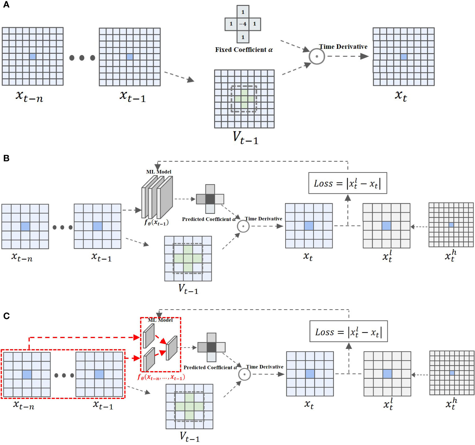
Figure 1 This figure shows three methods used to solve the spatial derivative during spatial discretization. (A) Figure 1(a) shows a traditional numerical method. (B) Figure 1(b) shows the deep-learning-based method. (C) Figure 1(c) shows our method. (A) The traditional numerical method: in the spatial discretization part, the central difference method is used to calculate the spatial derivative with a fixed spatial discretization coefficient, and then the temporal derivative is calculated in the temporal discretization process to obtain the numerical solution. (B)The Deep-learning-based method: In the spatial discretization part, predict the spatial discretization coefficient and calculate the spatial derivative based on the deep learning algorithm and the grid value at time t-1, and then calculate the temporal derivative in the temporal discretization process to obtain a numerical solution. (C). Our method: In the spatial discretization part, predict the spatial discretization coefficient and calculate the spatial derivative based on the deep learning algorithm and the grid value of the time series {t − n, …, t − 1}, and then calculate the time derivative in the time discretization process to obtain a numerical solution.

$\begin{array}{ll}SD={\sum }^{}\alpha V(x_{neigborhood},t-1)& (1)\end{array}$

where SD is the calculated spatial derivative, and V is a template composed of values at points around x within a certain distance at time t-1 α are fixed coefficients with regard to the corresponding truncation error Lantz (1971). Here, to capture the very subtle variations that occur in the physical movement of unsteady flow, traditional methods usually adopt grids with very high resolution, which leads to an extremely large computation cost. However, the deep-learning method addresses this problem by adopting large-scale grids with adaptively adjusted coefficients instead of traditional methods that adopt small grids with fixed coefficients, as shown in Figure 1B.

$\begin{array}{ll}SD={\sum }^{}{f}_{\theta }(x_{t-1})V(x_{neigborhood},t-1)& (2)\end{array}$

However, these previously proposed deep-learning-based methods predicted the coefficients only considering spatial correlation among grids, which provided relatively limited context and thus could not describe patterns along the temporal dimension sufficiently, implying that the spatiotemporal correlation of coefficients was not well learned. We propose a novel algorithm to extract grid correlations from spatial and temporal views together to address this problem. We simply illustrate our algorithm in Figure 1C. In our neural network, we added temporal neighborhoods to help predict grid coefficients:

$\begin{array}{ll}SD={\sum }^{}{f}_{\theta }(x_{t-1},x_{t-2},\dots )V(x_{neigborhood},t-1)& (3)\end{array}$

where {x_t−n,…,x_t−1} denotes grid values along the time dimension within a certain range. By adding temporal consideration, we can learn a better mapping function to predict the spatial grid coefficients and achieve a more accurate simulation result. Moreover, we also find that the concentration field, which was used as one of the inputs of the neural network, turns out to be redundant after we add temporal data. Thus, we optimized our method and produced a more efficient neural network with fewer parameters and better accuracy.

Thus, in this paper, we propose a novel time-sequence-involved space discretization neural network (TSI-SD) by taking temporal influence into consideration, which achieves an accurate and efficient simulation result of unsteady flow. Specifically, we produced the proposed neural network based on a classic CONV-LSTM backbone with careful modification by adding temporal information into two-dimensional spatial grids along the x-axis and y-axis separately at the first step and then fusing them together through a post-fusion neural network. After that, we combined the TSI-SD with the finite volume format as an advection solver for passive scalar advection in a two-dimensional unsteady flow. Compared with previous methods that only consider spatial context, our method can achieve higher simulation accuracy, while computation is also decreased after redundant input is removed.

Finally, we highlight the contribution of this paper as follows:

● We optimized the framework of the deep-learning-based numerical simulation methods of unsteady flow. As far as we are aware, we are the first to utilize the temporal relationship to help predict spatial coefficients. Moreover, we also simplified the neural networks by means of decreasing the parameter’s scale. Quite simply, our method achieved better accuracy and efficiency compared with existing methods.

● We designed a novel neural network TSI-SD and produced an effective spatial coefficients prediction method that takes both temporal and spatial perspectives into consideration. Our novel framework modeled spatial correlations and temporal correlations and then combined the two aspects properly with a well-designed post-fusion neural network.

● Comprehensive comparisons and ablation studies were carried out with three public datasets, i.e., the numerical solution datasets of the advection equation based on the Vanleer format under the random velocity field, deformed flow velocity field, and the constant velocity field. Sufficient results and explanations were provided and discussed to verify the improvement in both the accuracy and efficiency of the proposed idea.

2 Related work

2.1 Traditional discretization methods of fluid flow simulation

Many researchers have made outstanding contributions in the field of traditional discretization methods of fluid flow simulation Bristeau et al. (1985); Ferziger et al. (2002); Peyret and Taylor (2012); Fletcher (2012); Toro (2013). Based on these theories, Molenkamp et al. Molenkamp (1968) calculated the numerical solution of the convection equation using various finite-difference approximations, and determined that only the Roberts–Weiss approximation convected the initial distribution correctly, but required a huge computational cost. Mikula et al. Mikula et al. (2014) proposed an inflow implicit/outflow explicit finite volume method based on finite volume space discretization and semi-implicit time discretization to solve advection equations. The basic idea is that outflows from cells are handled explicitly, and inflows are handled implicitly. The method achieved outstanding results in terms of stability and computational accuracy. Zhao et al. Zhao et al. (2019) proposed a new improved finite volume method for solving one-dimensional advection equations under the framework of the second-order finite volume method. The method first applied the scalar conservation law to the elements in the finite volume method (FVM) to ensure its conservation in time and space and to ensure advection (i.e., conservation of transport physical quantities); then the time integral values of adjacent grid boundaries are equalized; finally, the equation is established to obtain a numerical solution. Experiments showed that this method has better stability and fewer disspation than the traditional FVM and can maintain the accuracy of the solution. Akitoshi Takayasu et al. Takayasu et al. (2019) proposed a verification calculation method for one-dimensional advection equations with variable coefficients, which was based on spectral methods and semigroup theory. They mainly provided a method for verification calculation using the C₀ semigroup on the complex sequence space l²,which comes from the solution of the Fourier series. Experiments showed that the given strict error proved the correctness of the exact solution, and the solution has high precision and fast solution speed. Although traditional discretization method shave achieved high solution accuracy, they have the problem of high computational cost if outstanding solution accuracy is desired.

2.2 Traditional discretization acceleration techniques for fluid flow simulation

To solve the problem of high computational cost while calculating high-precision solutions in traditional discretization methods, researchers have proposed acceleration techniques to speed up the numerical discretization solution. Multigrid technology stood out among various approaches Dwyer et al. (1982); Brown (1982); Berger and Oliger (1984); Phillips and Schmidt (1984); Phillips and Schmidt (1985); Zhang (1997); Mazhukin et al. (1993); Jin et al. (2014). Among them, Brown et al. Brown (1982) used the multigrid mesh-embedding technique to solve three-dimensional transonic potential flow. They used small grids to model regions of large local gradients and large-scale grids to model regions with relatively small gradients. Their method improved the speed of solving equation discretization schemes. Phillips et al. Phillips and Schmidt (1984) proposed a multilevel multigrid method combined with a Taylor series interpolation scheme as the best discretization acceleration scheme after comparing the use of simple multigrid and multilevel multigrid methods. Based on the previous method, Phillips Phillips and Schmidt (1985) used multigrid combined with multilevel acceleration technology to realize the accelerated solution of scalar conservation equations. In addition, they proposed a fast finite difference solution to the passive scalar advection-diffusion equation. Although these acceleration methods reduced the computational cost while maintaining high accuracy, high computational cost remained a problem due to the need to retain high solution grid modeling in some complex fluid regions.

2.3 Discretization methods and acceleration techniques combining deep-learning with traditional numerical methods

In recent years, machine learning has been used in the numerical solution of partial differential equations, which have made enormous progress. The combination of machine learning and traditional discretization methods improved the accuracy of the solution and accelerated the numerical calculation Raissi et al. (2019); Ji et al. (2021); Vinuesa and Brunton (2021); Patel et al. (2021); Eliasof et al. (2021); Cai et al. (2022). Based on these methods, O. Obiols-Sales et al. Obiols-Sales et al. (2020) proposed a coupled deep learning and physics simulation framework (CFDNet) to accelerate the convergence of Reynolds-averaged Navier–Stokes simulations. CFDNet was designed to use a single convolutional neural network at its core to predict the main physical properties of fluids, including velocity, pressure, and eddy viscosity. In this paper, CFDNet was evaluated for various use cases, and the results showed that CFDNet significantly speeded up the numerical solution and proved that CFDNet generalized well. Vadyala Shashank Reddy et al. Vadyala et al. (2022) determined the numerical solution of the one-dimensional advection equation using different finite-difference approximations and physical informatic neural networks (PINNs). They trained a neural network to solve supervised learning tasks that obeyed any given laws of physics described by general non-linear partial differential equations. The PINNs approximation was compared with other schemes through experiments, and the results showed that the prediction results obtained by the PINNs approximation were the most accurate. Pathak et al. Pathak et al. (2020) proposed a hybrid ML-PDE solver that combined machine learning and traditional solving methods of the partial differential equation. It can obtain meaningful high-resolution solution trajectories while solving system PDEs at lower resolutions. The ML part of the solver extracted spatial features by using u-net as the model structure to predict the error accumulated in the short time interval between the evolution of the coarse grid and the solution of the system at a higher resolution. The predicted error can optimize the solution generated by the coarse grid to obtain a solution close to that generated by the fine grid, enabling high-precision solutions at low accuracy. Y. Bar-Sinai Bar-Sinai et al. (2019) designed a data-driven discretization scheme using a deep-learning algorithm. They used neural networks to estimate spatial derivatives that were optimized end-to-end to best satisfy equations on low-resolution grids. The resulting numerical method was very accurate, eventually achieving the same computational accuracy as the standard finite difference method at 4 to 8 times coarser resolution than the standard finite difference method. Zhuang [38] improved the model structure and loss function based on Y. Bar-Sinai and applied it to passive scalar advection in a two-dimensional unsteady flow. They used a convolutional neural network to learn spatial discretization coefficients to calculate spatial derivatives. Then, they combined them with traditional numerical methods to calculate time derivatives to obtain the numerical solution of partial differential equations. This method achieved a high-precision solution with a low computational cost. Ranade et al., 2021 developed DiscretizationNet, a machine learning-based PDE solver that combined essential features of existing PDE solvers with ML techniques. They used a discretization-based scheme to approximate spatiotemporal partial derivatives and a CNN-based generative encoder-decoder model with PDE variables as input and output features for iteratively generating equation solutions. Although these methods addressed the problem of traditional methods, their solution accuracy was limited due to the problems of ignoring spatiotemporal characteristics and input redundancy.

3 Proposed method

3.1 Problem description

If the velocity field is divergence-free, the advective form of the scalar concentration field $C(\overrightarrow{x},t)$ for a given velocity field $\overrightarrow{u}(\overrightarrow{x},t)$ is as follows Zhuang et al. (2021):

$\begin{array}{ll}\frac{\partial C}{\partial t}+\overrightarrow{u}·\nabla C=0& (4)\end{array}$

The objective of the numerical solution for the passive scalar advection in 2-D unsteady flow is to predict the concentration field distribution at each time step in the future under the influence of the randomly changing velocity field given the initial concentration field. In this paper, we predict the concentration field distribution results in the 32 time steps to demonstrate the ability of our model to make multi-step predictions. We employ a rolling forecasting scheme in which we input multiple velocity fields between t₀ and t₁ into the prediction model and combine the concentration field distribution at t₀ to predict the concentration field distribution at t₁ .Then, we input multiple velocity fields between t₁ and t₂ into the model and combine the concentration field distribution at t₁, predicted by our model to predict the concentration field distribution at t₂. According to this calculation rule, we use multiple velocity fields between t_n and t_n+1 and the concentration field distribution predicted at time t_n to predict the concentration field distribution at t_n+1.By repeating this process, we can get the passive scalar advection solution at each time in the future. Therefore, the key to our multi-step prediction method is to recursively predict the concentration field distribution at a single step, i.e., the numerical solution of passive scalar advection at the next time step. We propose the time-sequence-involved space discretization neural network (TSI-SD) to predict the space discretization coefficient for the space derivative and then combine the finite volume method to calculate the numerical solution of the next time step.

3.2 Main framework of TSI-SD

The framework of the proposed method is shown in Figure 2. This is a fusion framework of deep learning (TSI-SD) and a traditional numerical method (FVM) for end-to-end numerical solutions of passive scalar advection equations. It consists of three modules: the spatial discretization coefficient prediction module (SDCPM), the concentration template extraction module (CTEM), and the concentration solver module based on finite volume numerical format (CSM). For the set of multiple velocity fields between the time steps t_n and t_n+1, wedecompose each velocity field into two sub-velocity fields in the horizontal and vertical directions (along the x-axis and y-axis) to obtain the velocity field set in the two directions. In the next step, we build the time-sequence-involved space discretization neural network (TSI-SD) in the SDCPM. TSI-SD extracts the spatiotemporal features from the decomposed velocity field sets in the two directions separately and then fuses them to obtain the spatial discretization coefficient of each grid point. After that, we input the coefficients into the CSM and combine them with the surrounding point concentration template of each grid point obtained by the CTEM to calculate the spatial derivative. Finally, we could calculate the concentration of each grid point at the next moment t_n+1,, that is, the concentration field of t_n+1 by the FVM in the CSM.

FIGURE 2

Figure 2 The framework of our approach. This framework is utilized for the solution of the passive scalar advection equation in a two-dimensional unsteady flow. It contains three modules: SDCPM, CTEM and CSM. SDCPM: This module receives multiple velocity field information at different times, extracts spatiotemporal features in two spatial dimensions (along the x-axis and y-axis), and finally fuses them in the spatial dimension to predict the spatial discretization coefficient of each grid point; CTEM: This module extracts the surrounding point concentration template of each grid point corresponding to the size of its spatial discretization coefficient template; CSM: This module calculates numerical solutions to the advection equations based on the finite volume method(FVM).

The equation-solving process can be roughly described in the following three steps:

1. Extract spatiotemporal features from the input velocity fields and predict spatial discretization coefficients;

2. Extract the surrounding point concentration template for each grid point; and

3. Fuse the predicted spatial discretization coefficient and the concentration template to obtain the spatial derivative, which is used to calculate the distribution of the concentration field, i.e., the numerical solution of the equation at the next time step by the finite volume method.

Next, we will provide details of our proposed framework for end-to-end numerical solutions of passive scalar advection equations. First, we introduce the SDCPM and the TSI-SD in the section entitled ‘Spatial Discretization Coefficient Prediction Module’. Then, we describe in detail our proposed CTEM and CSM modules in the Concentration Template Extraction Module’ and ‘Concentration Solver Module Based on Finite Volume Numerical Format’ sections, respectively. Finally, we discuss the loss function in the ‘Loss Function’ section 3.6

3.3 Spatial discretization coefficient prediction module

In this module, we design the time-sequence-involved space discretization neural network to predict the spatial discretization coefficients, and the prediction function is

$\begin{array}{ll}\overrightarrow{\alpha }=f(U,W),& (5)\end{array}$

where U s the set of multiple two-dimensional velocity fields between t nd t+1, of which size is nW s the weight of our neural network. The time interval between the velocity fields is $\frac{1}{n}$

$\begin{array}{ll}U=\left\{u_t,u_{t+\frac{1}{n}},\dots ,u_{t+1-\frac{1}{n}}\right\}& (6)\end{array}$

We decompose U into velocity field groups U_x in the horizontal direction (along the x-axis) and U_y in the vertical direction (along the y-axis),

$\begin{array}{ll}{U}_x=\left\{u_t^x,u_{t+\frac{1}{n}}^x,\dots ,u_{t+1-\frac{1}{n}}^x\right\}& (7)\end{array}$

$\begin{array}{ll}{U}_y=\left\{u_t^y,u_{t+\frac{1}{n}}^y,\dots ,u_{t+1-\frac{1}{n}}^y\right\}& (8)\end{array}$

Then, we extract the spatiotemporal features separately for the decomposed velocity field sets in the two directions. Taking U_x as an example, we input the velocity field at each time step from the velocity field set $\left\{u_t^x,u_{t+\frac{1}{n}}^x,\dots ,u_{t+1-\frac{1}{n}}^x\right\}$as the spatial feature of each time step into the different conv-lstm structural unit,

$\begin{array}{ll}{S}_k=u_k^x,& (9)\end{array}$

and S_k is regarded as the spatial feature at time $t+\frac{1}{k}$. A CONV-LSTM structural unit contains convolution operations and long-short-term memory unit processing operations. The calculation steps can be written in the following form,

$\begin{array}{ll}{i}_k=Sigmoid(Conv(S_k;w_{xi})+Conv(h_{k-1};w_{hi})+b_i)& (10)\end{array}$

$\begin{array}{ll}{f}_k=Sigmoid(Conv(S_k;w_{xf})+Conv(h_{k-1};w_{hf})+b_f)& (11)\end{array}$

$\begin{array}{ll}{g}_k=Tanh(Conv(S_k;w_{xg})+Conv(h_{k-1};w_{hg})+b_g)& (12)\end{array}$

$\begin{array}{ll}{c}_k=f_k\odot c_{k-1}+i_k\odot g_k=f_k·c_{k-1}+i_k\odot g_k& (13)\end{array}$

$\begin{array}{ll}{o}_k=Sigmoid(Conv(S_k;w_{xo})+Conv(h_{k-1};w_{ho})+b_o)& (14)\end{array}$

$\begin{array}{ll}{h}_k=o_k\odot Tanh(c_k)& (15)\end{array}$

where i_k is the input gate, which is used to calculate how much information of the current state to retain. f_x is the forget gate, and its function is to calculate how much of the output information of the previous moment is discarded. g_x is theinformation extracted from the current state. C_k-1 is the information of the previous moment. C_k is the final state at the current moment, calculated by f_k, c_k-1, g_k, and i_k. o_ki the output gate, which is used to calculate how much information needs to be output (to the cell at the next moment). h_k is the final output information of the state, which is calculated by o_k and c_k. w_xi,w_hi,w_xf,w_hf,w_xg,w_hg,w_xg,w_ho,b_i,b_f,b_g,and b_o are the weights designed in our neural network, and these weights will be updated during the model training process.

After the information processing and transmission of n conv-lstm structural units, the information $h_{t+1-\frac{1}{n}}$ output by the last unit is obtained. The final spatiotemporal fusion information I_x of the horizontal velocity field is calculated by using the output information.

$\begin{array}{ll}{I}_x=conv(h_{t+1-\frac{1}{n}})& (16)\end{array}$

In the same way, we obtain the final spatiotemporal fusion information I_y f the vertical velocity field.

After obtaining the spatiotemporal fusion information I_x and I_y in two directions, it is necessary to re-fuse the spatiotemporal features in the horizontal and vertical directions on I_x and I_y concat(), is a feature merging operation that integrates two features in a new dimension. After the feature merging operation, convolution is performed on the merged features to process the spatial information of the merged spatiotemporal features. Finally, the spatial discretization coefficient matrix α is obtained.

$\begin{array}{ll}\alpha =conv(concat(I_x,I_y))& (17)\end{array}$

The dimension of the α matrix is (s,s,template_size*2) , where s is the side length of the input two-dimensional velocity field, and (s, s) is the dimension of the two-dimensional velocity field. template_size is the number of weights required for each grid point. We divide α into the grid upper boundary space discretization coefficient α_up and the grid right boundary space discretization coefficient α_right with dimensions (s, s, template_size).

3.4 Concentration template extraction module

This module and the next module follow the numerical solution part of the traditional advection equation adopted by Zhuang et al. Zhuang et al. (2021), and adopt the spatial derivative of the classical Euler algorithm.

$\begin{array}{ll}\frac{\partial C}{\partial x}{\mid }_{x=x_i}=\sum _{j=0}^n{\alpha }_j{C}_{i+j}& (18)\end{array}$

In the previous part, we calculated the spatial discretization coefficient templates α_up and α_right, the dimensions of which are (s, s, template_size). Therefore, we need to find the surrounding grid point concentration templates C_up and C_right corresponding to the position of the coefficient template, the dimensions of which are both (s, s, template_size), which indicates that the number of surrounding grid point concentrations required for each point in the two-dimensional space field is template_size. As shown in Figure 3, we input the two-dimensional concentration field C_t at time t, and its dimension is (s, s). We model the upper and right boundaries of each point in the two-dimensional matrix and obtain the concentration values of m*n grid points around it as the grid point concentration template, where

FIGURE 3

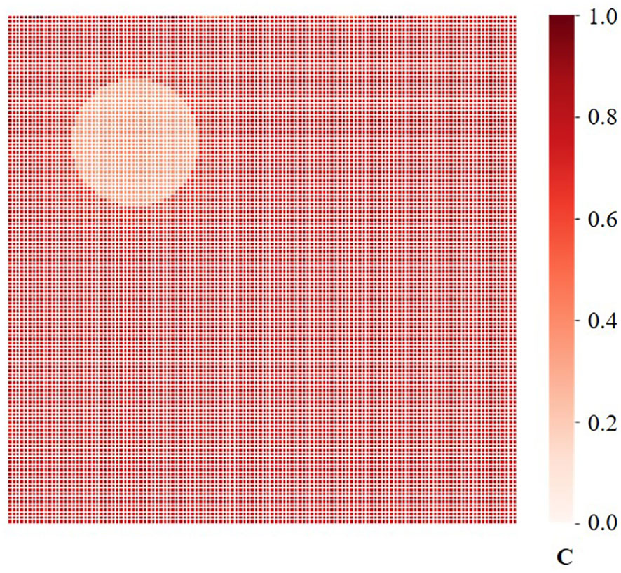
Figure 3 Design of the initial concentration field. The size of the concentration field is [0,1]×[0,1], and the concentration value is between 0 and 1.

$\begin{array}{ll}template\_size=m*n,& (19)\end{array}$

m and n are the length and width of the two-dimensional grid point concentration template. Finally, we obtain C_up and C_right with dimensions (s, s, template_size).

3.5 Concentration solver module based on finite volume numerical format

In this module, we first calculate the upper boundary concentration C_{up_edge} and the right boundary concentration C_{up_edge}

$\begin{array}{ll}{C}_{up\_edge}=SUM({\alpha }_{up}\odot C_{up})& (20)\end{array}$

$\begin{array}{ll}{C}_{right\_edge}=SUM({\alpha }_{right}\odot C_{right})& (21)\end{array}$

SUM() is the defined summation of the last dimension of the matrix, i.e., after the matrix of (s, s, template_size) is obtained through the dot product operation, the last dimension is summed to obtain the boundary concentration C_edge with dimension size (s, s) .The lower boundary concentration C_{lower_edge} and the left boundary concentration C_{left_edge} of the grid point can be directly obtained from the upper boundary concentration of the adjacent grid below its position and the right boundary concentration of the adjacent grid to the left of its position. Then, we can obtain the boundary velocity u_edge bythe same method as the calculation of the concentration boundary and boundary flux via C_edge u_edge. After obtaining the flux at the four boundaries of the grid, the traditional finite volume method is used to calculate the time derivative to obtain the concentration field distribution at the next time step, as shown in Figure 2.

3.6 Loss function

The format of the mean absolute error (MAE) used to train our model is as follows:

$\begin{array}{ll}MAE=\frac{1}{n}\sum _{i=1}^n\mid {\widehat{C}}_{t+1}-C_{t+1}\mid & (22)\end{array}$

where C_t+1 is the concentration field at time t+1 redicted by our model, and ${\widehat{C}}_{t+1}$ is the high-precision numerical solution at 16*16 low resolution grids. The numerical solution is calculated using 128*128 high resolution grids by the second-order Vanleer format and then transformed to the solution at 16*16 low resolution grids by the dimensionality reduction method Zhuang et al. (2021).

4 Experiments

In this section, we first briefly describe the datasets and implementation details. Additionally, we carry out a number of experiments, including comparisons with state-of-the-art (SOTA) methods and sufficient ablation studies, to demonstrate the excellent performance and advantages of our method.

4.1 Datasets

We used the theory of divergence-free velocity field described by Saad and Sutherland (2016) to generate a divergence-free random velocity field set with the resolution of 128*128. Then, the set was divided into two parts of divergence-free random velocity field sets: the training part and the test part. These two parts were completely different to ensure the generalization of the model.

For the training set, we generated a variety of random initial concentration fields and used the second-order Vanleer numerical format to calculate the numerical solution of the equation, i.e., the concentration fields at multiple time steps with the resolution of 128*128 based on the set of divergence-free random velocity fields in the training part. It is worth noting that for the C_t+1) to be generated, our model needs to input the velocity field i at time $t,t+\frac{1}{n},\dots ,t+1-\frac{1}{n}$. Therefore, we set the time step length of the velocity field to be smaller than the concentration field in the generation process to ensure that the velocity field in the time interval from t to t+1 could be generated. Next, we sampled both the velocity field and the concentration field at intervals to obtain a high-precision velocity field and concentration field with a resolution of 16*16 using the dimensionality reduction method Zhuang et al. (2021). Each training sample included an input part and an output part. The input part was the velocity field and the concentration field C_t at time t at multiple time steps in the time interval from t to t+1,and the output part was the concentration field C_t+1. The test set generation process was consistent with the training set, but it was necessary to ensure that the random initial concentration field generated in the test set was different from the training set.

The initial and boundary conditions for the velocity and concentration fields were set as follows. The size of the two-dimensional velocity field and the two-dimensional concentration field were both [0,1] × [0,1]. Our velocity field was a divergence-free random velocity field, and the magnitude of the velocity was limited between -1 and 1. The concentration field used periodic boundary conditions, and its initial condition is to

set the concentration value range between 0 and 1. The calculation process is shown in formulas (23)-(27).

$\begin{array}{ll}r(x,y)=min(1,4*\sqrt{{(x-\frac{1}{4})}^2+{(y-\frac{1}{4})}^2})& (23)\end{array}$

$\begin{array}{ll}{C}_1(x,y)=\frac{1}{2}[1+cos(\pi r)]& (24)\end{array}$

$\begin{array}{ll}{C}_2(x,y)=0.9-0.8*C_1^2& (25)\end{array}$

$\begin{array}{ll}{C}_3(x,y)=1& (26)\end{array}$

$\begin{array}{ll}C(x,y)=1-0.3*(C_1+C_2+C_3)& (27)\end{array}$

The C(x, y) is as shown in Figure 3. C represents the concentration value.

4.2 Comparison with SOTA methods

In this part, four SOTA numerical solution methods for passive scalar advection in a two-dimensional unsteady flow were selected as our baseline: (1) traditional solvers based on 16*16 resolution grids using the second-order Vanleer discretization format(Vanleer 16*16) Lin et al. (1994); (2) traditional solvers based on 32*32 resolution grids using the second-order Vanleer discretization format (Vanleer 32*32) Lin et al. (1994); (3) traditional solvers based on 64*64 resolution grids using the second-order Vanleer discretization format (Vanleer 64*64) Lin et al. (1994); and (4) a hybrid solver based on a CNN and the finite volume method (CNN+FVM) Zhuang et al. (2021).

We first compared our TSI-SD method with traditional solvers, in which TSI-SD uses a 16*16 low-resolution grid. As shown in Figure 4, the TSI-SD method maintained the smallest prediction error over 32 time steps, which demonstrates that our method achieved a higher solution accuracy than the traditional method at a resolution of 4× lower than the traditional method.

FIGURE 4

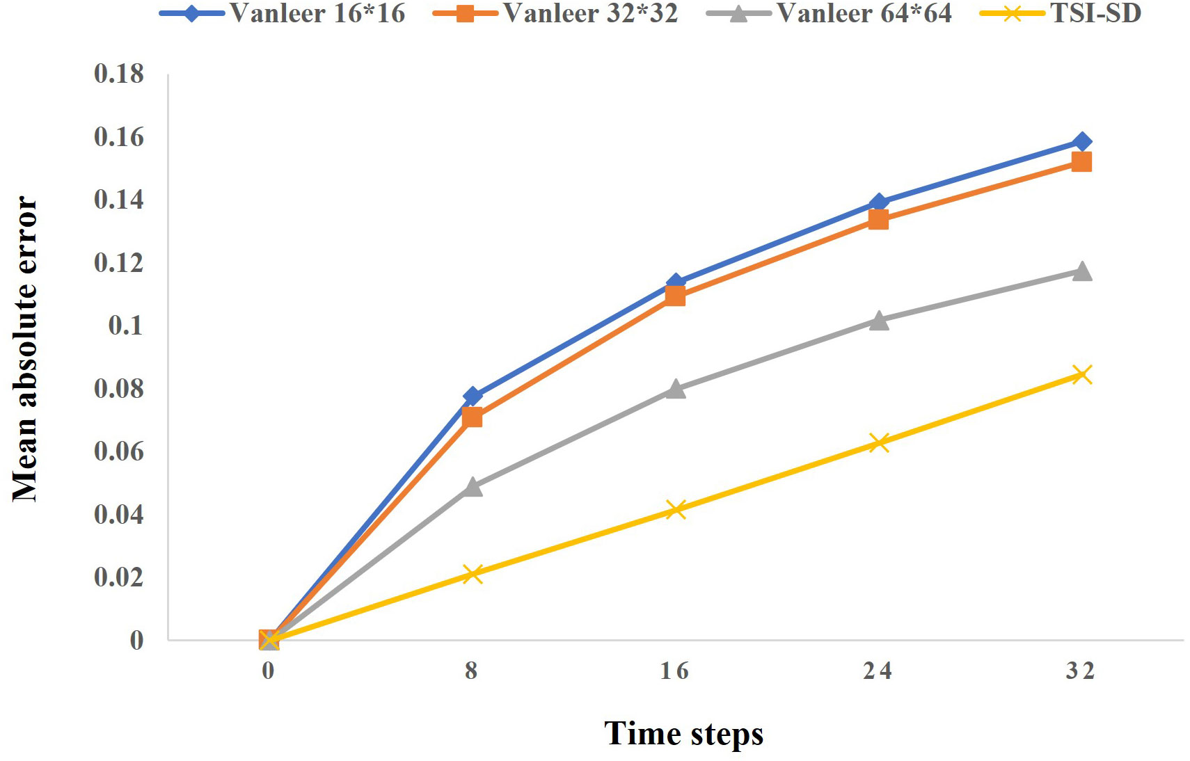
Figure 4 Results of our solver compared to traditional solvers. The yellow line represents our error in the 32-step iteration prediction, and the remaining three lines represent the error of the traditional solver at different resolutions.

Then, we compared TSI-SD with the CNN-FVM solver trained based on the previous spatial discretization scheme Zhuang et al. (2021). The CNN-FVM method is currently one of the most outstanding methods for solving partial differential equations in deep learning. It has been proven to achieve very good prediction and solution results in various partial differential equations, such as Burgers’ equation Bar-Sinai et al. (2019), and the advection equation Zhuang et al. (2021), Additionally, the method has been proven effective at solving complex Navier–Stokes equations Kochkov et al. (2021),and results are as accurate as baseline solvers, with 8–10× finer resolution in each spatial dimension, resulting in 40- to 80-fold computational speedups. The original CNN-FVM solver has a prediction error of 0.0043, a single-step prediction time of 0.2712s, and a single-sample training time of 4 ms per round during the training process. Our single-step solver had an error of 0.0029, a single-step prediction time of 0.2474s, and a single-sample training time of 2ms per round during training. Our single-step error was 32.56% lower than the previous method, and the iterative prediction error after 32 steps was greatly reduced. As shown in Figure 5, our method also outperformed the CNN-FVM solver in continuous prediction results within 32 time steps.

FIGURE 5

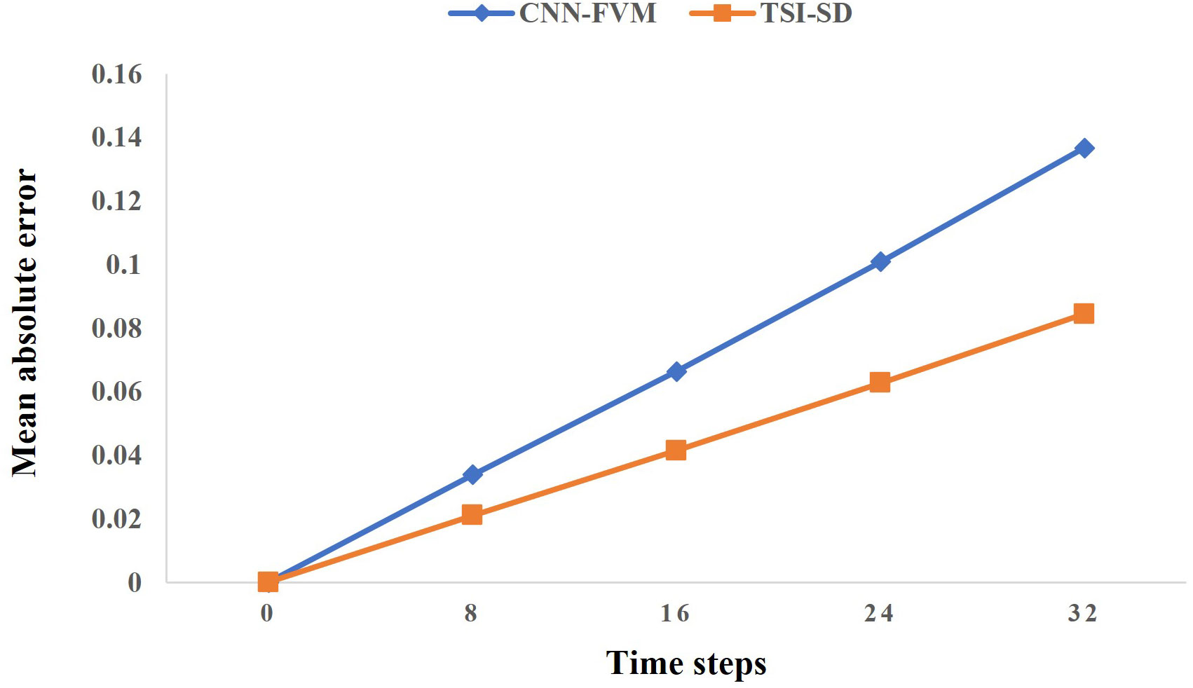
Figure 5 Results of our solver compared to CNN-FVM solvers by Zhuang Zhuang et al. (2021). The orange line represents our error in the 32-step iteration prediction, and the blue line represents the error of CNN-FVM solver.

The reason why our solver outperformed the CNN-FVM solver in training time, prediction time, and prediction accuracy is as follows. In the spatial discretization coefficent prediction part, the inputs of the CNN solver’s prediction deep-learning model are the concentration field with (batch_size,1,grid,_size,grid_size) and the two velocity field (along the x-axis and y-axis) at a time step with (batch_size,2,grid,_size,grid_size). The input to our TSI-SD was the horizontal velocity fields along the x-axis at two time steps with (batch_size,2,grid,_size,grid_size) and the vertical velocity fields along the y-axis at two time steps with (batch_size,2,grid,_size,grid_size), so our input size was larger than the previous input size. However, in the model part, the CNN-FVM solver used a five-layer convolutional neural network to process the data collected by the concentration field and the velocity field with (batch_size,3,grid,_size,grid_size) .We used the structure of a 1-layer

convolutional neural network to process the horizontal and vertical velocity fields respectively, and then a one-layer convolutional neural network was used to process the integrated features. After inference analysis, our model parameters were fewer than the original model parameters, which resulted in a shorter training time and prediction time in our model compared with the original model training time. This was also confirmed by a saved parameter file size comparison.

Finally, we demonstrated the evolution prediction effect of an initial concentration field under different models after 32 iterations. As shown in Figure 6, the third row shows the prediction effect of our model. The first row is our high-precision numerical solution generated using a 128*128 high-resolution grid. The second row shows how we use the averaging operation to obtain a high-precision numerical solution at a low resolution of 16*16, which is used as the ground truth of our model. The fourth and fifth rows are the results obtained using the second-order Vanleer 16*16 and CNN-FVM solvers. Figure 5 shows that our model is better than the CNN-FVM and traditional second-order Vanleer 16*16 solvers. In Figure 6, C represents the concentration value.

FIGURE 6

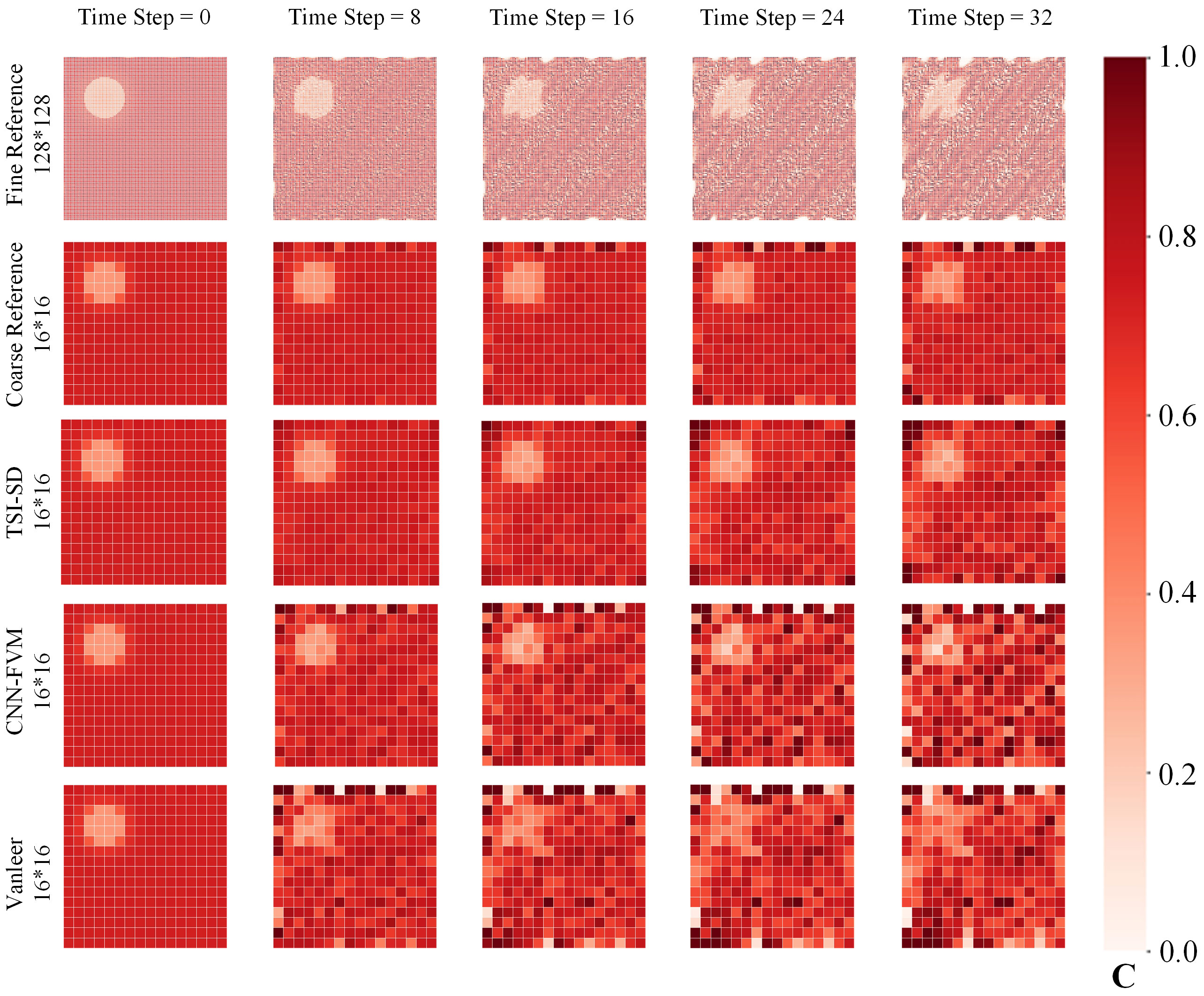
Figure 6 Visualization of evolution prediction effect of an initial concentration field under different models after 32 iterations. The first row represents the change in the concentration field calculated after 32 steps using a traditional 128*128 high-resolution solver. The second row represents the transformation of the 128x128 high-resolution solver solution into a 16x16 training set. The third row represents the prediction results of our model after training. The fourth row represents the prediction results of the CNN-FVM solver. The fifth row uses a traditional 16*16 low-resolution solver to calculate the change in the concentration field after 32 steps.

4.3 Comparison between models using velocity fields at different times as spatiotemporal features

In this part, we used different sets of time steps as the time series information input to TSI-SD, so that our model could extract different time features to predict the spatial discretization coefficient. The best prediction result represents the velocity fields at the selected time steps that have the greatest influence on the coefficients. Figure 7 shows that when the set of fine velocity fieldd $\left\{u_t,u_{t+\frac{1}{n}},\dots ,u_{t+1-\frac{1}{n}}\right\}$ was selected to replace velocity field set {u_t−n+1,…,u_t−1,u_t} to predict u_t+1 could reduce the prediction error of the model. The experimental result demonstrates that the set of fine velocity fields extracts spatiotemporal features more effectively. That is because the time interval of the velocity field set we chose was close to the time of the predicted concentration field, so the correlation between the velocity field set and the predicted concentration field was strong. The model could learn the spatiotemporal influence of the velocity field on the concentration field from this set of velocity fields, which could accurately predict the spatial discretization coefficient. Meanwhile, the prediction error of the velocity field using $\left\{u_t,u_{t+\frac{1}{2}}\right\}$ is the best, and experiments demonstrated that it involves lower computational cost; therefore, so we finally choose the

FIGURE 7

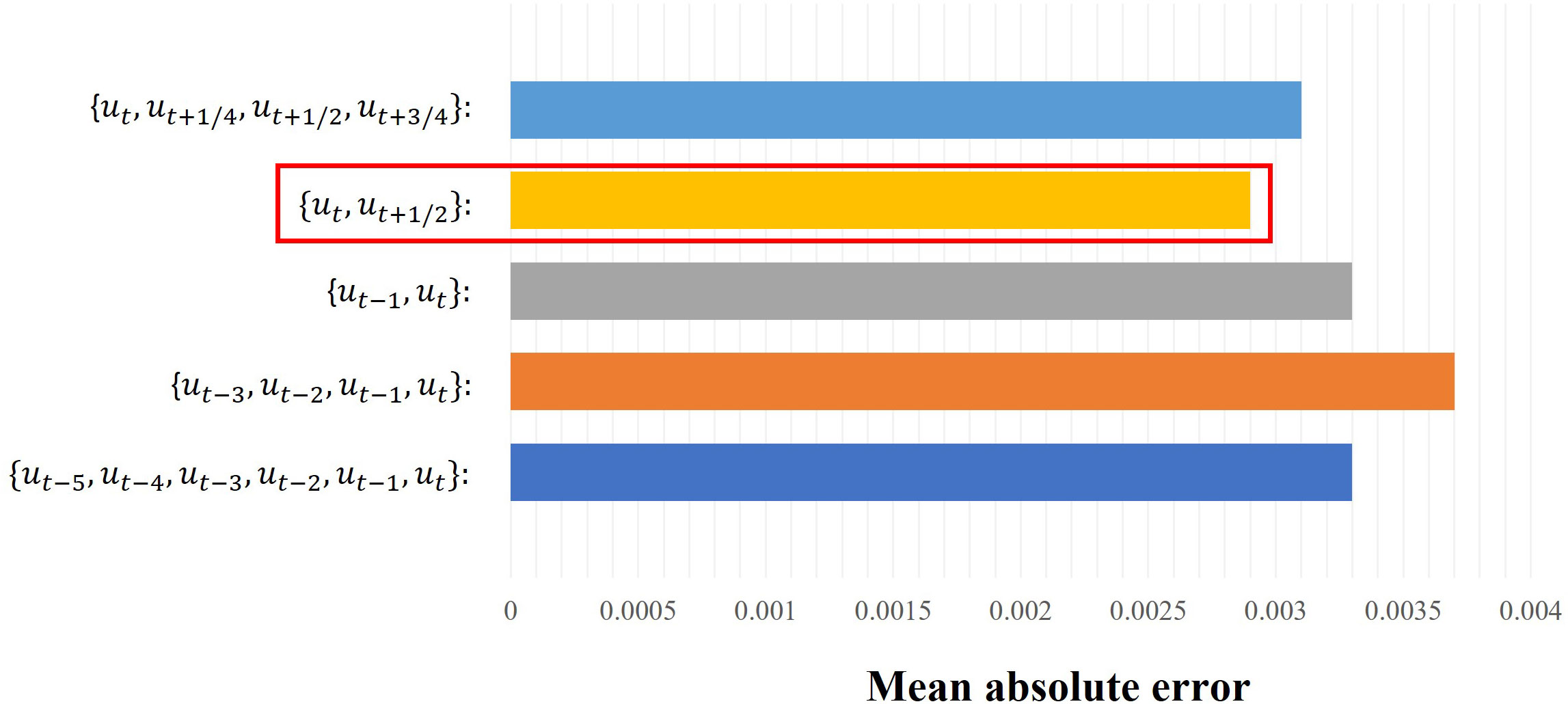
Figure 7 Mean absolute error comparison of the prediction results of models using different sets of time steps as the time series information input to TSI-SD. For the y-axis, the different colors represent different input sets of time steps. The legend represents mean absolute error and the red box shows the best result ( $\left\{u_t,u_{t+\frac{1}{2}}\right\}$).

velocity field of $\left\{u_t,u_{t+\frac{1}{2}}\right\}$ as the velocity field input of our final model. We think that for the 16*16 lower resolution grid, the model learned the time-space correlation between the velocity field set and the concentration field well through the analysis of the velocity fields at two times through a large amount of training data, which is also consistent with the experimental results as shown. In future studies, we will conduct more experiments on higher-resolution grids to obtain the optimal number of time steps after increasing computing power.

4.4 Performance and analysis of TSI-SD with other flow fields

In this section, we carried out an experiment to prove the excellent performance of our model under a constant velocity field and a two-dimensional deforming flow velocity field. We generated the concentration under a constant velocity field, and the two-dimensional deformation flow concentration field under the velocity field:

$\begin{array}{ll}u(x,y,t)=si{n}^2(\pi x)sin(2\pi y)cos(\frac{\pi t}{T})& (28)\end{array}$

$\begin{array}{ll}v(x,y,t)=si{n}^2(\pi y)sin(2\pi x)cos(\frac{\pi t}{T})& (29)\end{array}$

The predicted performance is shown in Figure 8 and Figure 9. C represents the concentration value. Our model achieved outstanding prediction results in the iterations of 32 time steps. However, at the same time,

FIGURE 8

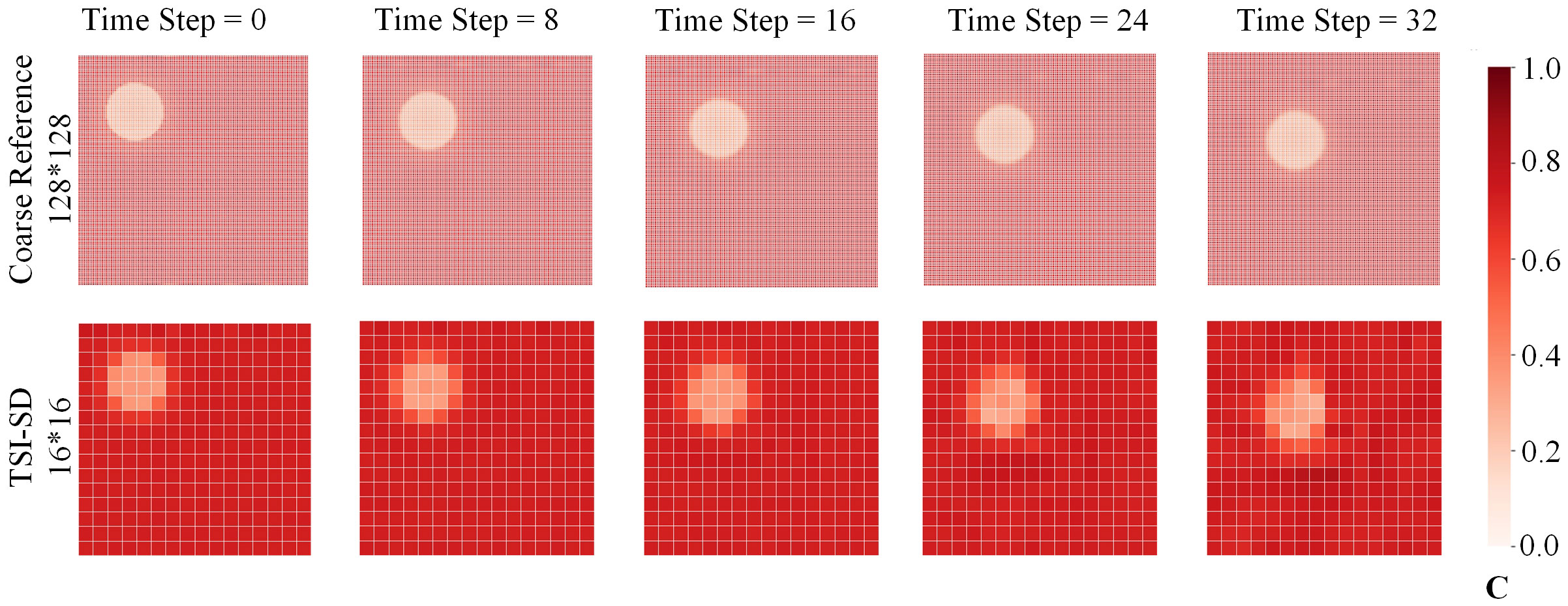
Figure 8 The predicted performance of our model in a constant velocity field of v_x=1 and v_y=1. The first row is the iterative solution of our 128*128 high-resolution solver after 32 time steps, and the second row is the iterative solution of our 16*16 solver after 32 time steps.

FIGURE 9

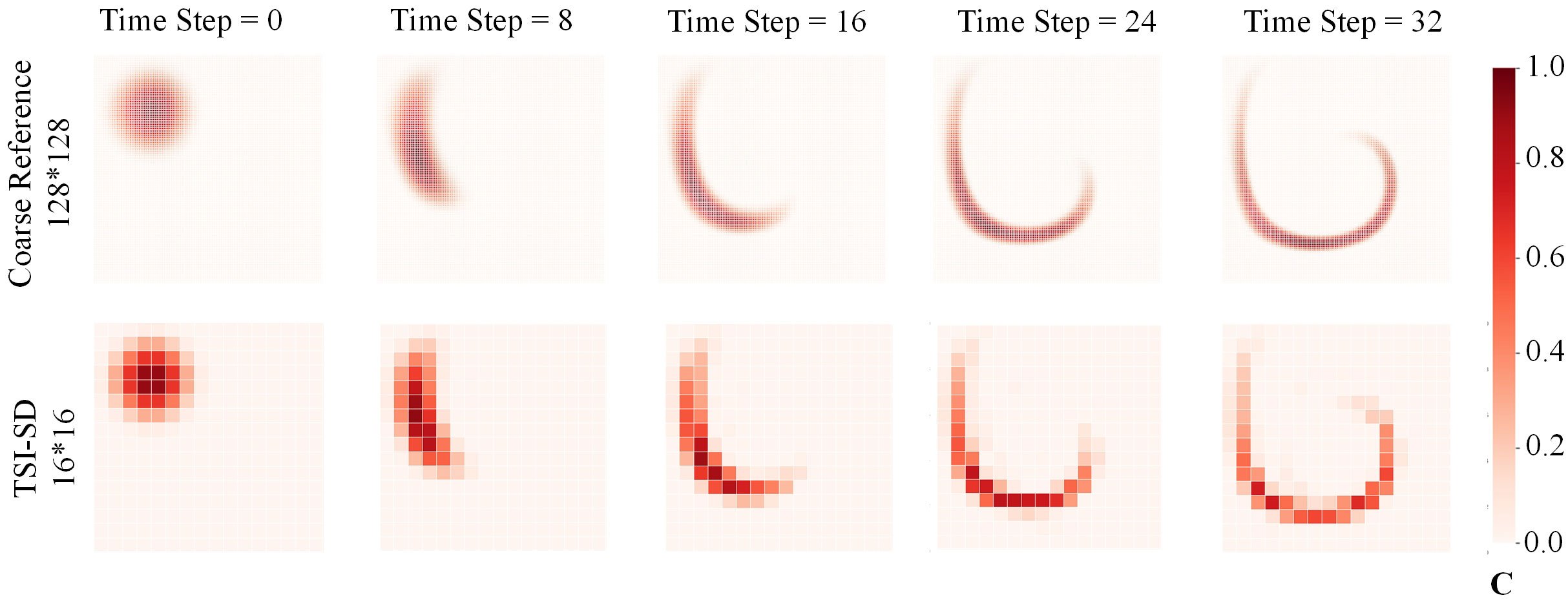
Figure 9 The predicted performance of our model in a deforming flow velocity field. The first row is the iterative solution of our 128*128 high-resolution solver after 32 time steps, and the second row is the iterative solution of our 16*16 solver after 32 time steps.

there are also the following problems: even under a simple constant velocity field, the prediction effect will become worse and worse with the long-term iteration due to the accumulation of errors predicted by the model at each time step. We will try to fix this in the future.

4.5 Comparison of the performance of models with or without the concentration field as an input feature

In this part, we verified the advantage of only taking the velocity field as the input feature on our model. A contrast model that adds the concentration field as feature input was designed to prove our inference. The contrast model was identical to ours except that the concentration field features were fused with the spatiotemporal features extracted from the horizontal and vertical velocity fields (along the x-axis and y-axis) in the fusion module. Figure 10 shows that the iteration errors on 32 time steps of our model are lower than those of the contrast model. Therefore, we proved that the input of the concentration field information was redundant and verified our conclusion: the spatial discretization coefficients are strongly correlated with the velocity field at multiple time steps before, while the concentration field information becomes redundant when predicting the coefficients. In other words, the change in the velocity field is the main factor for the change in the concentration field. Our model extracts effective spatiotemporal features from the velocity field set to learn the influence of the change of the velocity field set on the change of the concentration field, which is very helpful for predicting the spatial discretization coefficient.

FIGURE 10

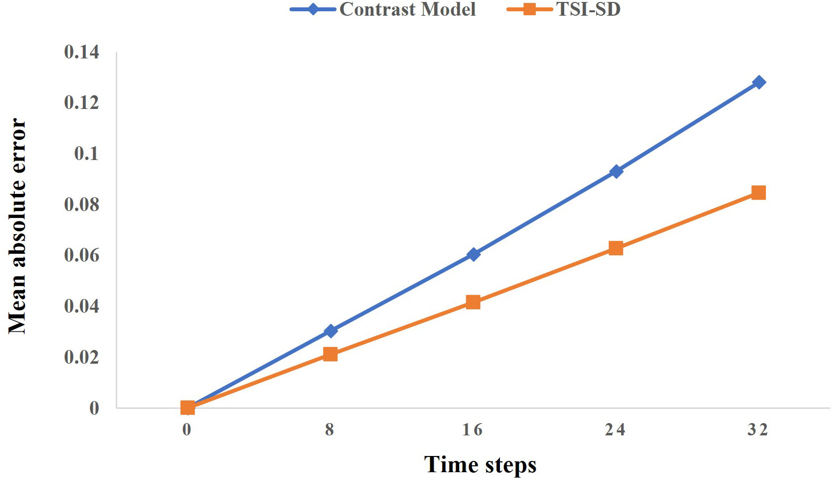
Figure 10 Results of our solver compared to the solver of adding concentration field as the model input. The orange line represents our error in the 32-step iteration prediction, and the blue line represents the error of the contrast model.

4.6 Experimental exploration of whether TSI-SD has up-wind properties

In this part, we proved that the spatial discretization coefficients predicted by our model have upwind properties on a constant velocity field. A two-dimensional velocity field U₁ with a horizontal velocity field (along the x-axis) of +1 and a vertical velocity field (along the y-axis) of +1, and a two-dimensional velocity field U₂ with a horizontal velocity field of -1 and a vertical velocity field of -1, were designed to prove our model’s upwind properties on a constant velocity field. Under the two velocity fields, the visualization process of the concentration coefficients of the upper and right boundaries of grid points A and B was completed.

As shown in Figure 11, C represents the concentration value and Coefficient represents the coefficient value. For the upper boundary, the concentration on the right boundary of the constant velocity field is mainly determined by the concentration of the two adjacent grids. When the horizontal speed is +1 (i.e., the direction is to the right), the grid coefficient on the left of the right boundary of grid A is greater than the grid coefficient on the right; when the horizontal speed is −1 (i.e., the direction is to the left), the grid coefficient on the left of the right boundary of grid A is smaller than the grid coefficient on the right. For the right boundary, the concentration on the upper boundary of the constant velocity field is also mainly determined by the concentration of the two adjacent grids. When the vertical speed is +1 (i.e., the direction is downward), the grid coefficient above the lower boundary of grid A is greater than the grid coefficient below; when the horizontal speed is −1 (i.e., the direction is upward), the grid coefficient above the lower boundary of grid A is smaller than the grid coefficient below.

FIGURE 11

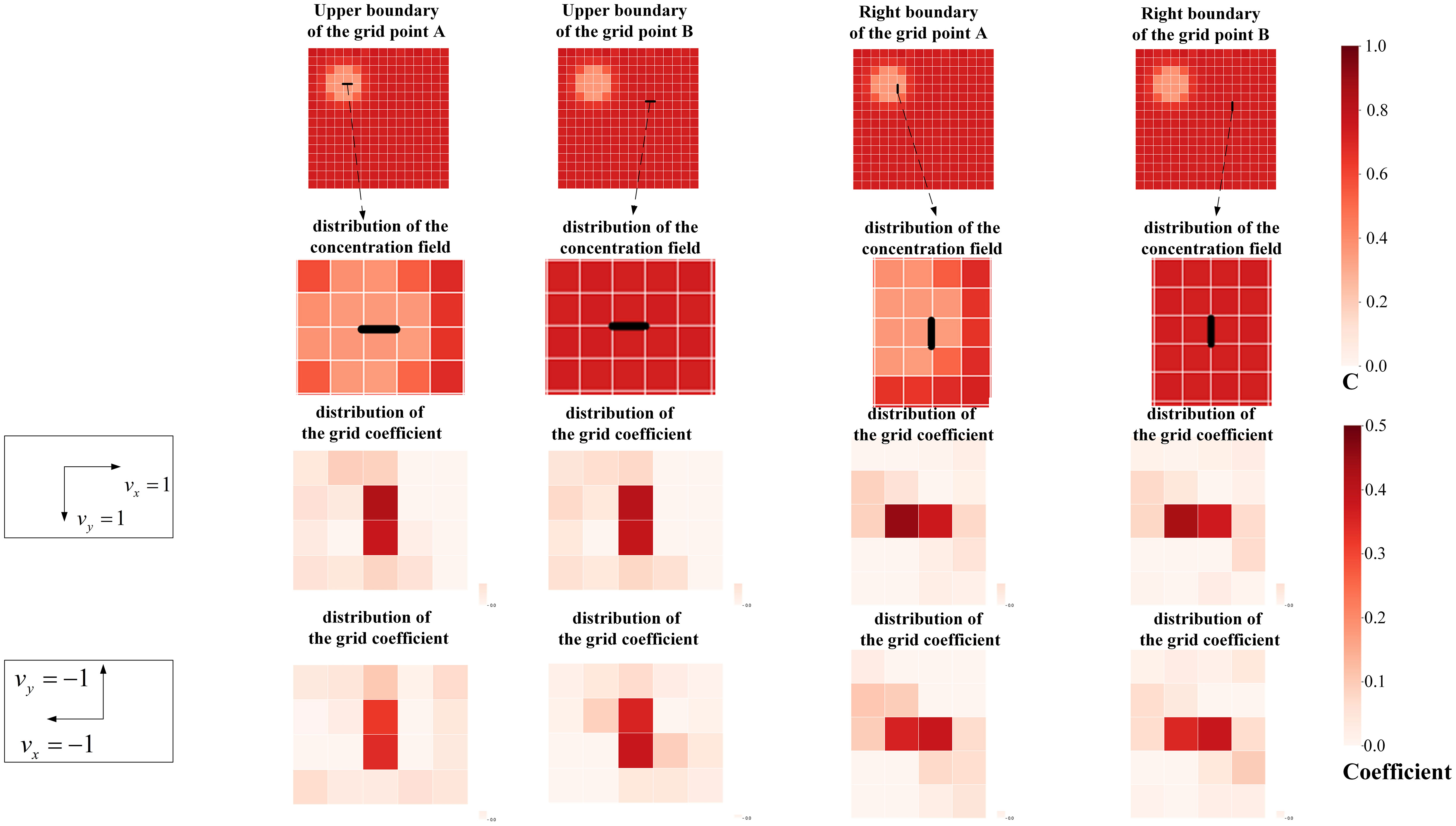
Figure 11 The comparison of prediction results of models using different temporal layers as features. The first line selects two spatial points with significant differences in surrounding concentrations from the spatial field and extracts the upper and right boundaries of the two points. The second row is the spatial discretization coefficient predicted by each boundary. The third row is a heat map made according to the different position coefficients in the coefficient template when the horizontal velocity field is +1, and the vertical velocity field is +1. The third row is a heat map made according to the different position coefficients in the coefficient template when the horizontal velocity field is -1, and the vertical velocity field is -1.

The concentration coefficient of another spatial grid point B is almost the same as that exhibited by A. Therefore, our grid coefficient has nothing to do with the distribution of the concentration field, but only with the distribution of the velocity field. The concentration field distributions at point A and point B are completely inconsistent, but under the same velocity field, the predicted spatial discretization coefficient distributions are basically the same, which proves that there is no significant correlation between the concentration field distribution and the spatial discretization coefficient.

5 Conclusion

We have presented a time-sequence-involved space discretization neural network of passive scalar advection in a two-dimensional unsteady flow. It can obtain adaptive spatial discretization derivatives according to the spatiotemporal property of the current environment. Then, we combined it with the finite volume method to form an advection equation solver that can calculate high-resolution solutions on low-resolution grids.

The highlight of our approach is the transformation of a novel deep neural network from the classic CONV-LSTM backbone. The network resolves spatiotemporal features by adding temporal information to a two-dimensional spatial grid along the x- and y-axes, and then fuses them through a post-fusion neural network. Through spatiotemporal feature fusion, we can predict more accurate spatial discretization coefficients and more accurate solutions. Additionally, we have made improvements in reducing computational costs. Finally, we compared our method with other traditional SOTA methods and demonstrated that it achieves better accuracy than traditional solvers on meshes with 4× lower resolution. In addition, compared with other deep-learning methods, our method has advantages in terms of both computational cost and accuracy.

The following problems were also encountered: (1) the problem of iterative error being too big after multiple time steps—we have proposed some solutions, such as re-iteration with ground-truth values after iterating over some time steps, which will be implemented in future work; and (2) low computing power leads to poor model generalization—in the future, we will seek to obtain more computing power to make our model more generalizable.

Data availability statement

The raw data supporting the conclusions of this article will be made available by the authors, without undue reservation.

Author contributions

NS carried out the methodology, data processing, modeling, and writing of the original draft. HT performed the conceptualization, validation, and review, and optimized the model framework. HG, JS, and YY performed the validation and investigation. ZW carried out the writing review. JN contributed to the conceptualization, writing review and editing, and supervision. All authors contributed to the article and approved the submitted version.

Funding

This work was supported in part by the National Key Research and Development Program of China (2021YFF0704000), the National Natural Science Foundation of China (62172376), and Fundamental Research Funds for the Central Universities (202042008).

Acknowledgments

We thank two reviewers for their useful comments. We are very grateful to Prof. Song (Dehai Song, Key Laboratory of Physical Oceanography, Ocean University of China, Qingdao, China) for providing us with data and ideological support and help.

Conflict of interest

The authors declare that the research was conducted in the absence of any commercial or financial relationships that could be construed as a potential conflict of interest.

Publisher’s note

All claims expressed in this article are solely those of the authors and do not necessarily represent those of their affiliated organizations, or those of the publisher, the editors and the reviewers. Any product that may be evaluated in this article, or claim that may be made by its manufacturer, is not guaranteed or endorsed by the publisher.

References

Bar-Sinai Y., Hoyer S., Hickey J., Brenner M. P. (2019). Learning data-driven discretizations for partial differential equations. Proc. Natl. Acad. Sci. 116, 15344–15349. doi: 10.1073/pnas.1814058116

CrossRef Full Text | Google Scholar

Berger M. J., Oliger J. (1984). Adaptive mesh refinement for hyperbolic partial differential equations. J. Comput. Phys. 53, 484–512. doi: 10.1016/0021-9991(84)90073-1

CrossRef Full Text | Google Scholar

Bristeau M., Pironneau O., Glowinski R., Periaux J., Perrier P., Poirier G. (1985). On the numerical solution of nonlinear problems in fluid dynamics by least squares and finite element methods (ii). application to transonic flow simulations. Comput. Methods Appl. Mechan Eng. 51, 363–394. doi: 10.1016/0045-7825(85)90039-8

CrossRef Full Text | Google Scholar

Brown J. (1982). “A multigrid mesh-embedding technique for three-dimensional transonicpotential flow analysis,” in 20th aerospace sciences meeting [Orlando, FL,U.S.A: American Institute for Aeronautics and Astronautics (AIAA)], 107. doi: 10.2514/6.1982-107.

CrossRef Full Text | Google Scholar

Cai S., Mao Z., Wang Z., Yin M., Karniadakis G. E. (2022). Physics-informed neural networks (pinns) for fluid mechanics: A review. Acta Mechan Sin. [Orlando, FL, U.S.A.: American Institute for Aeronautics and Astronautics (AIAA)], 1–12. doi: 10.1007/s10409-021-01148-1

CrossRef Full Text | Google Scholar

Dwyer H. A., Smooke M. D., Kee R. J. (1982). Adaptive gridding for finite difference solutions to heat and mass transfer problems (Fort Belvoir, Virginia: California Univ Davis Dept Of Mechanical Engineering).

Google Scholar

Eliasof M., Haber E., Treister E. (2021). Pde-Gcn: Novel architectures for graph neural networks motivated by partial differential equations. Adv. Neural Inf. Process. Syst. 34, 3836–3849. doi: 10.48550/arXiv.2108.01938

CrossRef Full Text | Google Scholar

Ferziger J. H., Perić M., Street R. L. (2002). Computational methods for fluid dynamics (Cham, Switzerland: Springer), 3.

Google Scholar

Fletcher C. A. (2012). Computational techniques for fluid dynamics: Specific techniques for different flow categories (Springer-Verlag Berlin Heidelberg New York: Springer Science & Business Media).

Google Scholar

Ji W., Qiu W., Shi Z., Pan S., Deng S. (2021). Stiff-pinn: Physics-informed neural network for stiff chemical kinetics. J. Phys. Chem. A 125, 8098–8106. doi: 10.1021/acs.jpca.1c05102

PubMed Abstract | CrossRef Full Text | Google Scholar

Jin M., Liu W., Chen Q. (2014). Accelerating fast fluid dynamics with a coarse-grid projection scheme. HVAC&R Res. 20, 932–943. doi: 10.1080/10789669.2014.960239

CrossRef Full Text | Google Scholar

Kochkov D., Smith J. A., Alieva A., Wang Q., Brenner M. P., Hoyer S. (2021). Machine learning–accelerated computational fluid dynamics. Proc. Natl. Acad. Sci. 118, e2101784118. doi: 10.1073/pnas.2101784118

CrossRef Full Text | Google Scholar

Kraichnan R. H. (1959). The structure of isotropic turbulence at very high reynolds numbers. J. Fluid Mechan 5, 497–543. doi: 10.1017/S0022112059000362

CrossRef Full Text | Google Scholar

Lantz R. (1971). Quantitative evaluation of numerical diffusion (truncation error). Soc. Petroleum Engineers J. 11, 315–320. doi: 10.2118/2811-PA

CrossRef Full Text | Google Scholar

Leschziner M. (1989). Modeling turbulent recirculating flows by finite-volume methods–current status and future directions. Int. J. Heat Fluid Flow 10, 186–202. doi: 10.1016/0142-727X(89)90038-6

CrossRef Full Text | Google Scholar

Lin S.-J., Chao W. C., Sud Y., Walker G. (1994). A class of the van leer-type transport schemes and its application to the moisture transport in a general circulation model. Monthly Weather Rev. 122, 1575–1593. doi: 10.1175/1520-0493(1994)122<1575:ACOTVL>2.0.CO;2

CrossRef Full Text | Google Scholar

Lumley J. L. (1979). Computational modeling of turbulent flows. Adv. Appl. mechanics 18, 123–176. doi: 10.1016/S0065-2156(08)70266-7

CrossRef Full Text | Google Scholar

Mazhukin V., Bobeth M., Semmler U. (1993). A dynamically adaptive grid method for solving one-dimensional non-stationary partial differential equations. (Dresden, Germany: Max-Planck-Gesellschaft zur Förderung der Wissenschaften eV). 1–18.

Google Scholar

Mikula K., Ohlberger M., Urbán J. (2014). Inflow-implicit/outflow-explicit finite volume methods for solving advection equations. Appl. Numerical Math. 85, 16–37. doi: 10.1016/j.apnum.2014.06.002

CrossRef Full Text | Google Scholar

Molenkamp C. R. (1968). Accuracy of finite-difference methods applied to the advection equation. J. Appl. Meteorol. Climatol. 7, 160–167. doi: 10.1175/1520-0450(1968)007<0160:AOFDMA>2.0.CO;2

CrossRef Full Text | Google Scholar

Obiols-Sales O., Vishnu A., Malaya N., Chandramowliswharan A. (2020). “Cfdnet: A deep learning-based accelerator for fluid simulations,” in Proceedings of the 34th ACM international conference on supercomputing (Barcelona, Spain), 1–12. doi: 10.1145/3392717.3392772

CrossRef Full Text | Google Scholar

Patel R. G., Trask N. A., Wood M. A., Cyr E. C. (2021). A physics-informed operator regression framework for extracting data-driven continuum models. Comput. Methods Appl. Mechan Eng. 373, 113500. doi: 10.1016/j.cma.2020.113500

CrossRef Full Text | Google Scholar

Pathak J., Mustafa M., Kashinath K., Motheau E., Kurth T., Day M. (2020). Using machine learning to augment coarse-grid computational fluid dynamics simulations. arXiv preprint arXiv:2010.00072. doi: 10.48550/arXiv.2010.00072

CrossRef Full Text | Google Scholar

Peyret R., Taylor T. D. (2012). Computational methods for fluid flow (New York, USA: Springer Science & Business Media).

Google Scholar

Phillips R., Schmidt F. (1984). Multigrid techniques for the numerical solution of the diffusion equation. Numerical Heat Transfer 7, 251–268. doi: 10.1080/01495728408961824

CrossRef Full Text | Google Scholar

Phillips R., Schmidt F. (1985). Multigrid techniques for the solution of the passive scalar advection-diffusion equation. Numerical heat transfer 8, 25–43. doi: 10.1080/01495728508961840

CrossRef Full Text | Google Scholar

Rai M. M., Moin P. (1991). Direct simulations of turbulent flow using finite-difference schemes. J. Comput. Phys. 96, 15–53. doi: 10.1016/0021-9991(91)90264-L

CrossRef Full Text | Google Scholar

Raissi M., Perdikaris P., Karniadakis G. E. (2019). Physics-informed neural networks: A deep learning framework for solving forward and inverse problems involving nonlinear partial differential equations. J. Comput. Phys. 378, 686–707. doi: 10.1016/j.jcp.2018.10.045

CrossRef Full Text | Google Scholar

Ranade R., Hill C., Pathak J. (2021). Discretizationnet: A machine-learning based solver for navier–stokes equations using finite volume discretization. Comput. Methods Appl. Mechan Eng. 378, 113722. doi: 10.1016/j.cma.2021.113722

CrossRef Full Text | Google Scholar

RUMSEY C., VATSA V. (1993). “A comparison of the predictive capabilities of several turbulence models using upwind and central-difference computer codes,” in 31st aerospace sciences meeting [Reno, NV, U.S.A.: American Institute for Aeronautics and Astronautics (AIAA)], 192.

Google Scholar

Saad T., Sutherland J. C. (2016). Comment on “diffusion by a random velocity field”[phys. fluids 13, 22 (1970)]. Phys. Fluids 28, 22. doi: 10.1063/1.4968528

CrossRef Full Text | Google Scholar

Takayasu A., Yoon S., Endo Y. (2019). Rigorous numerical computations for 1d advection equations with variable coefficients. Japan J. Ind. Appl. Math. 36, 357–384. doi: 10.1007/s13160-019-00345-7

CrossRef Full Text | Google Scholar

Toro E. F. (2013). Riemann Solvers and numerical methods for fluid dynamics: a practical introduction (Springer-Verlag Berlin Heidelberg New York: Springer Science & Business Media).

Google Scholar

Vadyala S. R., Betgeri S. N., Betgeri N. P. (2022). Physics-informed neural network method for solving one-dimensional advection equation using pytorch. Array 13, 100110. doi: 10.1016/j.array.2021.100110

CrossRef Full Text | Google Scholar

Vinuesa R., Brunton S. L. (2021). The potential of machine learning to enhance computational fluid dynamics. arXiv preprint arXiv:2110.02085. doi: 10.1038/s43588-022-00264-7

CrossRef Full Text | Google Scholar

Zhang J. (1997). Multigrid acceleration techniques and applications to the numerical solution of partial differential equations (The George Washington University).

Google Scholar

Zhao S., Zhou J., Jing C., Li L. (2019)Improved finite volume method for solving 1-d advection equation (IOP Publishing) (Accessed Journal of Physics: Conference Series).

Google Scholar

Zhuang J., Kochkov D., Bar-Sinai Y., Brenner M. P., Hoyer S. (2021). Learned discretizations for passive scalar advection in a two-dimensional turbulent flow. Phys. Rev. Fluids 6, 064605. doi: 10.1103/PhysRevFluids.6.064605

CrossRef Full Text | Google Scholar