 Yuhang Zheng
 Wei Zhuang
 Yan Du
- 1State Key Laboratory of Marine Environmental Science, College of Ocean and Earth Sciences, Xiamen University, Xiamen, China
- 2State Key Laboratory of Tropical Oceanography, South China Sea Institute of Oceanology, Chinese Academy of Sciences, Guangzhou, China
- 3College of Marine Science, University of Chinese Academy of Sciences, Beijing, China
The tropical western Pacific and the adjacent South China Sea are home to many low-lying islands and coastal zones that are vulnerable to flood hazards resulting from extreme sea level (ESL) changes. Based on the hourly sea level recorded by 15 tide gauges during the period 1980-2018, this study evaluates the historical trend of ESLs over this region. On this basis, a regression model for hourly future sea-level prediction is established by combining the atmospheric reanalysis products, the tidal harmonics, and the outputs of three climate models archived by the Coupled Model Intercomparison Project Phase 6 (CMIP6) to evaluate the future ESL changes in 1.5 °C and 2.0 °C warmer climates. The historical trend of ESLs show that the ESLs along the coasts and islands of the tropical western Pacific have significantly risen during the past decades, which is mainly contributed by the mean sea level rise. And results from the historical observations and the prediction model show that in a warming climate from 1980 to 2050, both the mean sea levels and ESLs rise with fluctuations. The mean sea level change plays an important role in the secular trend of ESLs, while the interannual-to-decadal variability of ESLs is significantly affected by tides and extreme weather events. Under the warming scenario of 1.5°C, the changes in the return levels of ESL relative to the historical period are generally small at most tide gauge sites. Compared with the situations under 1.5°C warming, the return levels of ESL at most selected tide gauges will rise more significantly under the 2.0°C warming scenario, so the frequency of the current 100-year return level will reduce to less than 10 years at most stations. The above results suggest that this additional 0.5°C warming will cause a huge difference in the ESLs along the coasts and islands of the tropical western Pacific. As proposed in the Paris climate agreement, it is very necessary to limit anthropogenic warming to 1.5°C instead of 2.0°C, which will substantially reduce the potential risk of flood disasters along the coasts and islands of the tropical western Pacific.
Introduction
The extreme sea level (ESL) is defined as the maximum sea level during a selected period, usually a year, and its variability is mainly triggered by the combined effects of mean sea level, tides, and storm surges (Marcos et al., 2015). For instance, strong ESL events often occur when high tides coincide with storm surges due to atmospheric forcing, often leading to the most hazardous coastal flooding and causing devastating damage to coastal ecosystems and human livelihoods (Vousdoukas et al., 2018). Therefore, in recent years, the changes in ESLs have been extensively investigated at both global and regional scales (e.g. Cayan et al., 2008; Feng et al., 2015; Feng and Jiang, 2015; Wahl et al., 2017; Rasmussen et al., 2018; Kirezci et al., 2020). There is considerable evidence that ESL has generally risen globally over the past few decades and that changes in ESL, especially its secular trend, are highly correlated with changes in mean sea level in many coastal regions (Marcos et al., 2009; Menéndez and Woodworth, 2010; Weisse et al., 2014). Meanwhile, future projections by climate models suggest that the increase in the occurrence frequency of ESL caused by anthropogenic warming is more significant in tropical oceans than in mid-high latitudes (Vousdoukas et al., 2018; Tebaldi et al., 2021).
The tropical western Pacific is characterized by the highest sea surface temperature in the global ocean, bearing frequent storms and typhoon activities. It is also a region containing strong variability of interannual-to-decadal climate modes, like El Niño and Southern Oscillation (ENSO) and Pacific Decadal Oscillations (PDO). Strong sea level variability, induced by storm surges, tides, and lower-frequency climate modes, leads to more coastal inundation in low-lying, highly-populated coastal regions of the tropical western Pacific. The tropical western Pacific contains many low-lying islands and coastal areas with heavy concentrations of population and economic activity, where the impact of ESL will be particularly severe for this region. Some studies on global ESL have already specifically depicted the ESL variability in the tropical western Pacific and adjacent Asian waters. Vousdoukas et al. (2018) predicted that compared with the status during 1980-2014, ESL in 2100 would increase by 57 cm in the southeast Asia waters and by 59 cm in the south Pacific, the highest rise in the globe, under the moderate warming scenario of RCP4.5. The work further pointed out that the rise in ESL was mainly driven by the thermal expansion of ocean water, followed by contributions from ice mass loss from glaciers and ice sheets in Greenland and Antarctica. Tebaldi et al. (2021) pointed out that in 2100, the frequency of the current 100-year return level will change to one year at most of the stations in the southeast Asia waters under the scenario of 1.5°C warming. Wahl et al. (2017) predicted that under RCP4.5, the frequency of the current 100-year return level in the tropical western Pacific islands would change to 1-5 years by 2050, and those in most stations along the tropical western Pacific coast would change to 5-20 years by 2050, only those in a small number of stations would change to 20-50 years.
The Paris Climate Agreement aims to hold global warming well below 2.0°C and to pursue efforts to limit it to 1.5°C above pre-industrial temperature. (UNFCCC, 2015a). However, a recent literature review under the United Nations Framework Convention on Climate Change (UNFCCC) found the notion that ‘up to 2.0°C of warming is considered safe, is inadequate’ and that ‘limiting global warming to below 1.5°C would come with several advantages (UNFCCC, 2015b)’. Recently, increasing studies have been performed to investigate the extreme climate events (i.e., ESL, marine heat wave, drought risk) at the 1.5°C and 2.0°C global warming, and most results indicated the superiority of limiting warming to 1.5°C rather than 2.0°C (Lehner et al., 2017; Dosio et al., 2018; Rasmussen et al., 2018; Feng et al., 2018b; Tebaldi et al., 2021). However, the difference in ESL under these two warming scenarios has not yet been well understood in the tropical western Pacific.
To further clarify the ESL characteristics in the western Pacific and the adjacent South China Sea (SCS), the return periods and return levels of ESLs were systematically investigated in this study using the tide gauge sea level observations, the atmospheric reanalysis products, and the state-of-the-art climate models. Particular attention is paid to the different ESL responses to 1.5°C and 2.0 °C warming levels. As the SCS is often treated as a part of the western Pacific, hereafter, we name the whole study region as the tropical western Pacific. The rest of this paper is organized as follows. Section “Data and Methods” describes the datasets and methods used in this study. In Section “Results”, we explore the historical ESL variability and the future ESL changes at 1.5°C and 2°C warming levels. Contributions of potential influential factors are also evaluated. Lastly, our results are summarized and discussed in Section “Conclusion and Discussion”.
Data and methods
Tide gauge data
The tide gauge sea level data used in this study are collected and distributed by University of Hawaii Sea Level Center, one of the primary data centers in the Global Sea Level Observing System. The accuracy and completeness of the data are critical for correct estimations of ESL changes. So only hourly Research Quality (RQ) data with more rigorous quality control are adopted in this study. Given that the earlier tide gauge data has lower completeness, we focused on the RQ data during the period January 1980 - December 2018 and required the time series to contain at least 25 years of data, resulting in 15 stations. The locations and names of the selected tide gauge stations are shown in Figure 1. In addition, obvious spurious records or abnormal data spikes in the sea-level time series of all tide gauges were checked by visual inspections and then further corrected or eliminated. For instance, in the sea-level records of a few stations (e.g. Hir, Lgp), an overall drift with anomalously large amplitude occurs after a certain point in time, probably due to the artificial relocation of tide gauge. To correct these abrupt sea-level shifts, the abnormal differences between adjacent records were replaced by the differences between their corresponding climatological mean values during 1980-2018.
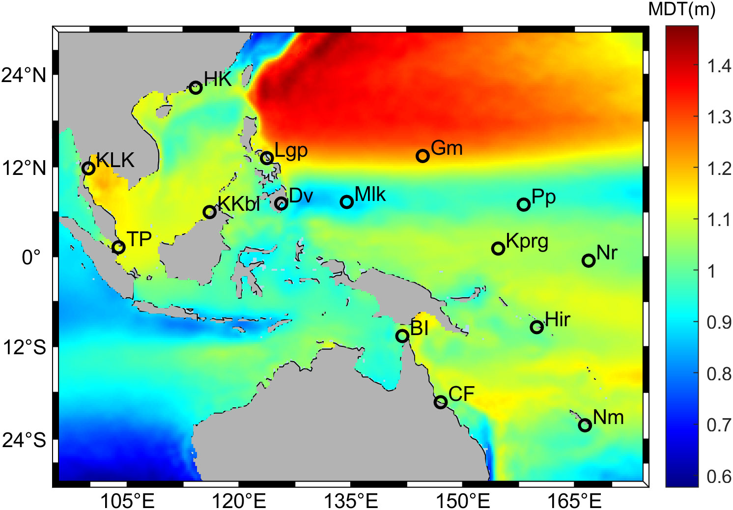
Figure 1 Mean dynamic topography over the study region based on the CNES-CLS18 dataset (Mulet et al., 2021) and the locations of 15 selected tide gauges: Pohnpei (Pp), Nauru (Nr), Malakal (Mlk), Honiara(Hir), Noumea (Nm), Kapingamarangi (Kprg), Guam (Gm), KoLaK (KLK), HongKong (HK), Booby Island (BI), Cape Ferguson (CF), Legaspi (Lgp), Davao (Dv), Kota Kinabalu (KKbl), Tanjong Pagar (TP).
Percentile analysis method and ensemble empirical mode decomposition
The percentile analysis method has been widely used to assess ESL changes (Marcos and Woodworth, 2017; Feng et al., 2018b; Feng et al., 2019). It gives the percentiles below which a certain percentage of the data in a dataset is found. In this study, this method is applied to extract 99.9%, 99%, and 90% percentiles of the observed sea level each year to reveal interannual and longer-term variability of ESLs.
The sea level tendency can be estimated by analyzing its oscillatory behavior, which means extracting periodic components from original observations successively until no periodic component is left (Jevrejeva et al., 2006). Due to the empirical, intuitive, direct, and adaptive characteristics, the empirical mode decomposition (EMD) method is suitable for estimating the accurate long-term trend of the sea level data (Huang et al., 1998; Huang et al., 1999). The EMD method decomposes an arbitrary time series X(t) into a finite and often small number of intrinsic mode functions (IMFs), defined as any function with an equal number of extreme and zero-crossing. Then X(t) can be described as:
where, n is the number of IMFs, and rn is the residual (Huang et al., 1998).
Ensemble empirical mode decomposition (EEMD) is the improved method to obtain IMFs with more direct physical meaning and greater uniqueness (Wu and Huang, 2009). EEMD was estimated by averaging numerous EMD runs with the addition of some white noise and has been widely used to get the long-term change of the mean sea levels recently (Chen et al., 2017; Feng et al., 2019; Ezer and Dangendorf, 2020). By averaging the different decompositions, the noise was averaged out and the true decomposition was calculated with a confidence estimate.
Extreme value analysis method
The risks associated with ESLs can be assessed from the estimates of return levels and return periods. Return level is defined as the sea level that occurs at a specific frequency. A return period refers to the average time between a specific sea-level return level being exceeded at a particular location. We obtained return levels and return periods by the transformed-stationary approach for non-stationary extreme value analysis (Mentaschi et al., 2016). The first step of this approach is the input of the initial ESL time series. We did this based on the classical annual maximum method, which defines the maximum values of each year in the hourly sea level time series as the ESLs. And the second step is to analyze the extreme value distribution of the input data. Compared with the traditional non-stationary extreme analysis method, this approach separates the detection of non-stationarity of the time series from the fitting of extreme distribution. It consists of (i) transforming a non-stationary time series into a stationary one, to which the stationary theory can be applied, and (ii) reverse transforming the result into a non-stationary extreme value distribution by means of some frequency analysis methods, such as the Gumbel, Weibull, and generalized extreme value (GEV) distributions. This study used the GEV distribution model to analyze the return levels of ESLs since it frequently outperforms other alternative methods (Feng and Jiang, 2015) and has been widely used to investigate various types of extreme events (Dosio et al., 2018; Vousdoukas et al., 2018; Takbash and Young, 2020). The detailed theoretical background and equations for the GEV distribution and the transformed-stationary approach can be found in Huang et al. (2008) and Mentaschi et al. (2016).
A model of hourly sea level
Since the prediction of future ESLs by extreme value analysis method requires hourly sea level data, this study adopted a two-stage procedure to realize the future ESL projections: first, an hourly regression model on sea level was established for each station based on the observational data and CMIP6 historical simulations; then, using these regression models, we projected future hourly sea level and evaluated the corresponding ESL variability under 1.5°C and 2.0°C warming scenarios. It has been pointed out that both atmospheric pressure effect and wind forcing can cause sea level change, and the greatest influence on short-period non-tidal sea level variability comes from inverse barometer effects, with wind stress contributing only incrementally (Cayan et al., 2008; Feng and Jiang, 2015; Muis et al., 2017). Following Vousdoukas et al. (2018), we define hourly sea level (HSL) as:
where, MSL represents the yearly-mean sea level, ηTIDE is the astronomical tide level, and ηCE is the water level fluctuations due to climate extremes, i.e., wind-waves and storm surges. The historical MSL is defined as the yearly-mean sea level computed from tide gauge data, and the future MSL is calculated mainly based on the dynamic sea level (labelled as ‘ZOS’) and the global mean thermosteric sea level change (labelled as ‘ZOSTOGA’) data provided by the CMIP6 models. The ‘ZOS’ and ‘ZOSTOGA’ data are de-drifted by removing their respective secular trends in the corresponding pre-industrial control runs. In addition, the influences of ocean mass change due to the freshwater imports from glaciers, Antarctic ice sheet, Greenland ice sheet, and land water have also been considered. The annual forecast values of these factors estimated in some previous studies are directly used in this study(Wada et al., 2012; Slangen et al., 2014; Marzeion et al., 2020; Edwards et al., 2021). The past and future ηTIDE are calculated by the tidal harmonic constants of 27 components given by the FES2014 tidal model (Lyard et al., 2021). For the historical period of 1980-2018, the values of HSL are directly derived from tide gauge observations, so the historical non-tidal sea level residuals ηres can be obtained by subtracting MSL and ηTIDE from HSL, and it corresponds to atmospherically forced ηCE in the Equation (2).
Following Cayan et al. (2008), we used the historical observations to establish one multiple linear regression model for each station that correlated ηres with the sea level fluctuations ηCE driven by local sea level pressure (SLP) and sea surface wind stress forcing. The hourly SLP and wind stress are derived from the ERA5 reanalysis dataset. The correlation coefficients and F-test statistics between the predicted ηCE and the calculated ηres are shown in Table 1. The general correlation coefficients of coastal stations (i.e., Nm, KLK, BI, CF) are mostly higher than those of islands. Some of them even exceed 0.7. Due to the large amount of data involved in the regression (at least 236688 hourly records in 39 years), the correlation coefficients of islands located in the open ocean (i.e., Pp, Nr, Mlk, Hir, Kprg) are relatively low but still reach more than 0.2. The F-test statistics of all 15 stations are much higher than the critical F value of 1.0, so the multiple linear regression model is generally significant. It can also be seen from Table 1 that the contribution ratios of SLP to ηCE at 15 stations are more than 97%, which, as also suggested by Cayan et al. (2008), reflects the dominant role of the barometric effect.
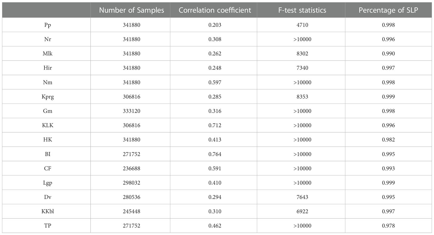
Table 1 The number of samples and the multiple linear regression model results for each tide-gauge station.
The future ηCE projection is mainly based on the SLP and wind stress simulated by three CMIP6 numerical models under ssp2-4.5 scenario (Table 2). We chose these three CMIP6 numerical models because their outputs contain all of the variables with the necessary temporal resolutions for sea level estimations. In addition, the historical simulations of these three models reasonably reproduce the mean and variance patterns of SLP and wind stress shown in the results of ERA5 reanalysis (Figures not shown). The future simulations of these three models begin in 2015. Since the model outputs only provide daily SLP and wind stress, the data need to be interpolated hourly to meet the requirement of future ηCE prediction. To synthesize hourly SLP and wind stress, we extracted the high-frequency signals with a period shorter than 24 hours from the hourly SLP and wind stress time series of the ERA5 product and interpolated these hourly time series to the corresponding daily outputs of CMIP6 models. Then, with reference to the ERA5 reanalysis data, the varying amplitudes of the interpolated data were adjusted proportionally to ensure that the variance of both datasets was the same. Then the interpolated SLP and wind stress data were input into the sea level regression model for each tide gauge station to predict the future hourly ηCE during 2015-2050. The HSL in the future was finally obtained by adding the predicted annual mean MSL and hourly ηTIDE and ηCE at each station through Equation (2).
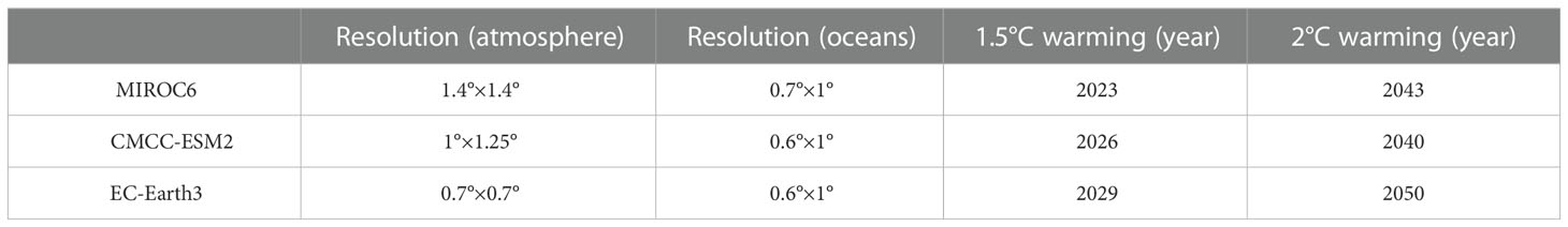
Table 2 The selected CMIP6 simulations and projected year of warming.
Results
Historical ESL variability
The 99.9%, 99%, and 90% levels of observed sea level have been calculated at all 15 tide gauges (Figure 2). The results show that the three percentile levels of each station are similar, but the fluctuation amplitude of ESL is the largest at 99.9% level and the smallest at 90% level. Except for Pp, KLK, Dv, and KKbl, the three percentile levels of ESL at all other stations rise with fluctuations. At the same time, the ESLs of all tide gauges show obvious interannual-to-decadal variability, among which the varying amplitudes at HK and BI stations are the most obvious, with a range of more than 0.3 m.
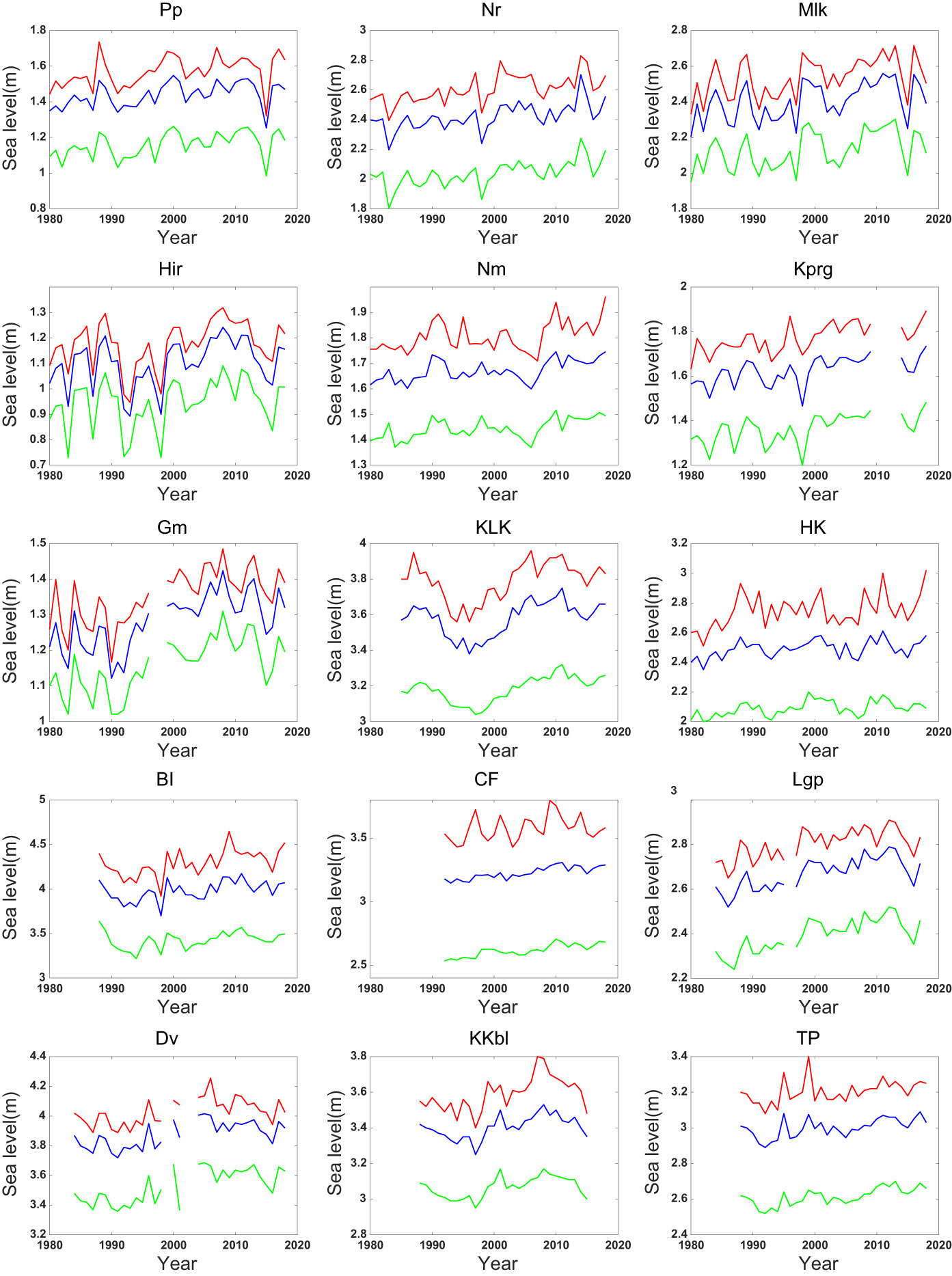
Figure 2 99.9% (red lines), 99% (blue lines), and 90% levels (green lines) of the observed sea levels at 15 tide gauges.
The EEMD method is used to further extract the long-term nonlinear trends of ESLs in coastal and island zones of the tropical western Pacific. As seen in Figure 3, ESLs along the coasts and islands of the tropical western Pacific generally present rising trends during 1980-2018. But the detailed tendency features of ESLs at different tide gauges are distinct. At Hir and KLK, the growing trends are almost linear. At Nm, Gm, BI, and CF, the growing trends are not obvious initially but strengthen gradually. At Nr, Mlk, Kprg, HK, Lgp, and Dv, the rising trends weaken gradually. At Pp, KKbl, and TP, the ESLs show obvious rising trends before 2005 and then shift to decline afterward. It should be noted that the long-term trend derived via EEMD method may be significantly influenced by extreme anomalies in some specific years. For example, at Pp, the decline trend after 2000 is primarily caused by the large negative anomalies of sea level in 2015.
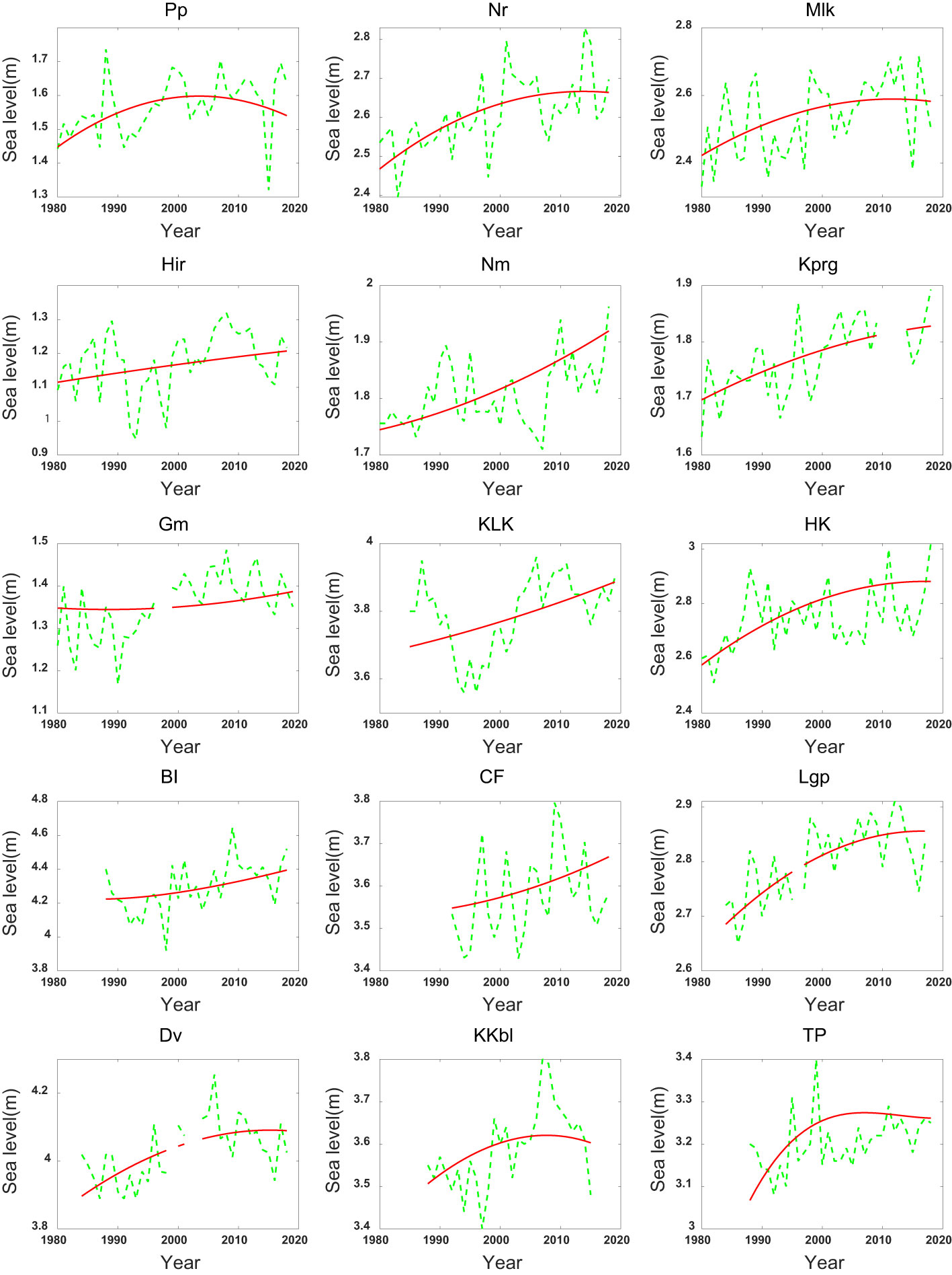
Figure 3 Long term trends of the ESLs at 15 tide gauges (red lines), 99.9% levels of the observed sea levels (green lines).
To evaluate the potential impacts of mean sea level variability on the ESL changes, this study calculates the correlations between the 99.9% percentile ESL and the yearly-mean sea level. The results in Table 3 suggest that the ESLs are significantly correlated with the mean sea level at most of the 15 tide gauges. The overall correlation for all stations is 0.736 (above the 99% confidence level). Generally, the correlation coefficients are relatively high for stations on small islands in the western Pacific Ocean and relatively low for stations on the coasts of continents or big islands. For instance, the stations with correlation coefficients higher than 0.85 (Pp, Nr, Mlk, Hir, Gm, Lgp, and Dv) are all located on relatively smaller islands. In contrast, correlations lower than 0.6 exist within the SCS (KLK and HK) and on the eastern Australian coast (CF). The CF station is the only one whose correlation coefficient does not exceed the 95% confidence level (Table 3). This regional contrast in correlation coefficients implies that the impact of year-mean sea level on the ESL variability looks more significant in the open ocean than in the coastal region.
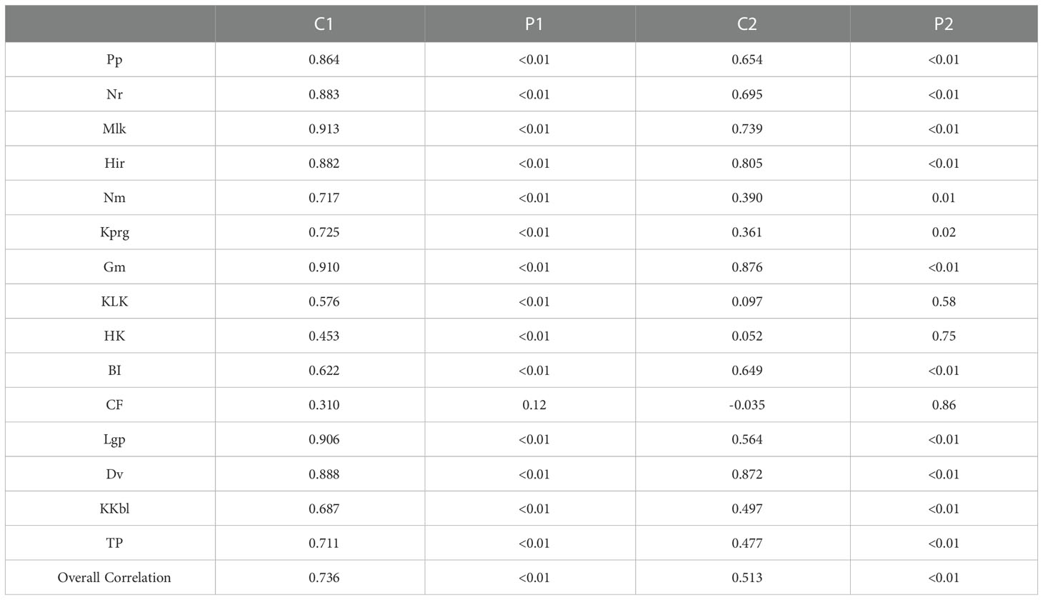
Table 3 Correlation coefficient between the ESL and mean sea level at 15 tide gauges (C1) and the correlations after getting rid of EEMD trends (C2), the P1/P2 are the p-value from t-test (where p < 0.05 means that the correlation was significant at 95% confidence level).
After the removal of EEMD trends, the correlation coefficients between ESLs and yearly-mean sea levels decrease at all tide gauges, suggesting that the long-term trends of ESLs are substantially contributed by the mean sea level trends, consistent with previous studies in other regions (Marcos et al., 2009; Weisse et al., 2014). The overall correlation coefficient reduces from 0.736 to 0.513, but remains above the 99% level. Besides CF station, the correlation coefficients for stations HK and KLK also reduce to below the 95% confidence level after detrending. It is worth mentioning that these three stations are located on the coastlines of continents, while the correlation coefficients of small islands located in the open ocean also decrease after detrending but are still above the 95% confidence level, indicating that mean sea level modulates not only to the secular ESL trend but also the interannual-to-decadal ESL variability during 1980-2018.
Projections of future ESLs under 1.5°C and 2°C warming scenarios
The 21st-century simulations of three climate models from CMIP6 are used to predict the future amplitudes of the global mean surface temperature. In all these models, the baseline for future warming estimations is initial warming of 1.1°C in 2015, derived from the HadCRUT5 global mean surface temperature difference between 2013-2017 and 1850-1900. The projections of three climate models consistently suggest that global warming will reach 1.5°C in the 2020s and 2.0°C during 2040-2050 (Table 2). CMCC-ESM2 simulation reaches 1.5°C in 2026 and 2.0°C in 2040, respectively. MIROC6 is the earliest to reach 1.5°C warming in 2023, but it reached 2.0°C warming later than CMCC-ESM2 in 2043. EC-Earth3 has the slowest warming rate, reaching 1.5°C in 2029 and 2.0°C in 2050.
The return levels and return periods of ESLs under different warming levels are further calculated by using the extreme value analysis method described above. Compared with the present-day status observed by tide gauges, the changes in return levels under the 1.5°C warming scenario are generally small (Figure 4). At some tide gauge stations (e.g., Nr, Nm, and Dv), the return levels estimated based on three climate models all show little changes relative to the observed present-day values. Under the 2.0°C warming scenario, however, the return levels of ESLs at most tide gauge sites increases substantially compared to the present-day scenario (Figure 5), suggesting a rapid intensification of ESL from the 2020s to 2040s.
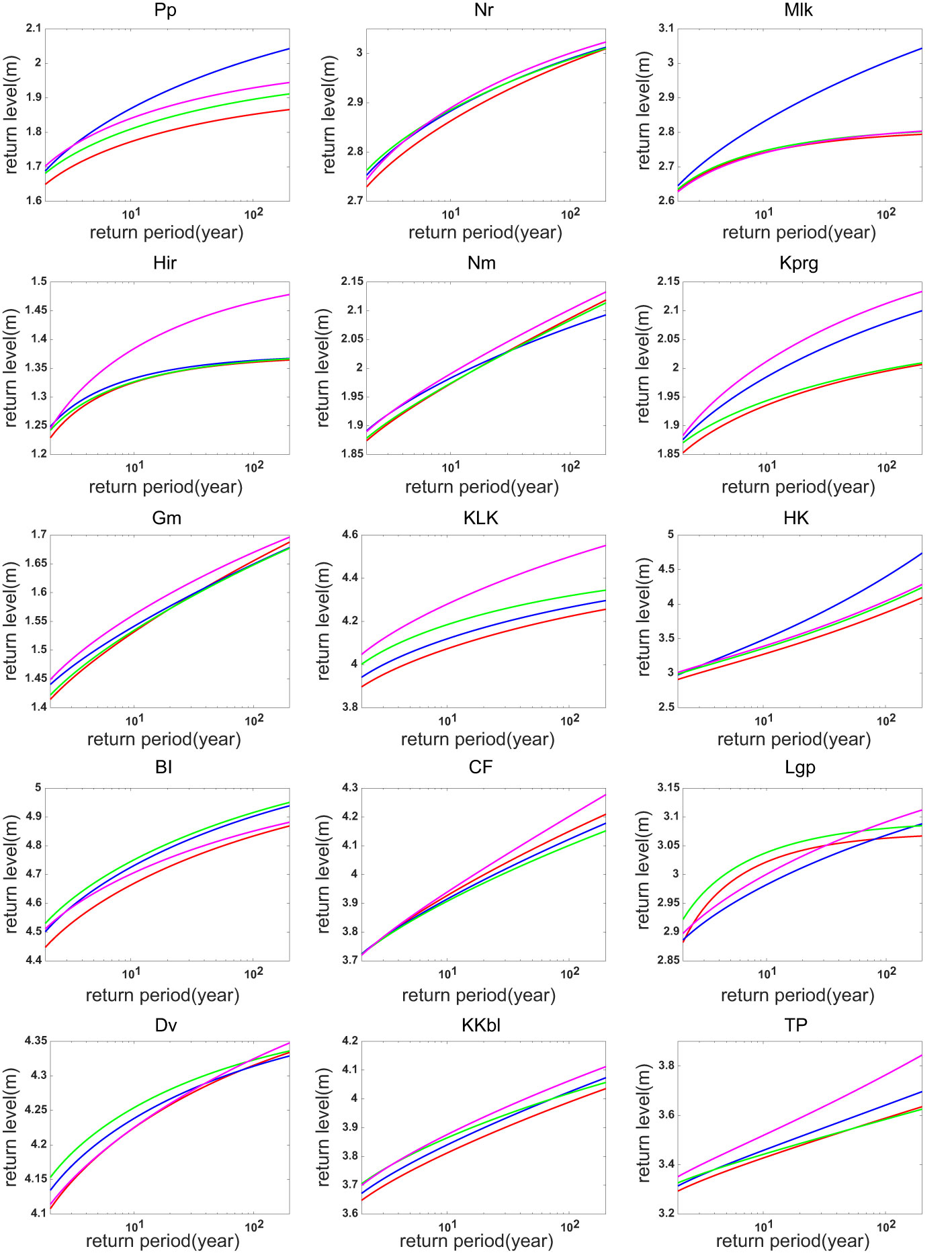
Figure 4 Return levels of the ESL at present (red line) and under the 1.5°C warming scenario: MIROC6 (blue line), CMCC-ESM2 (green line), EC-Earth3 (pink line).
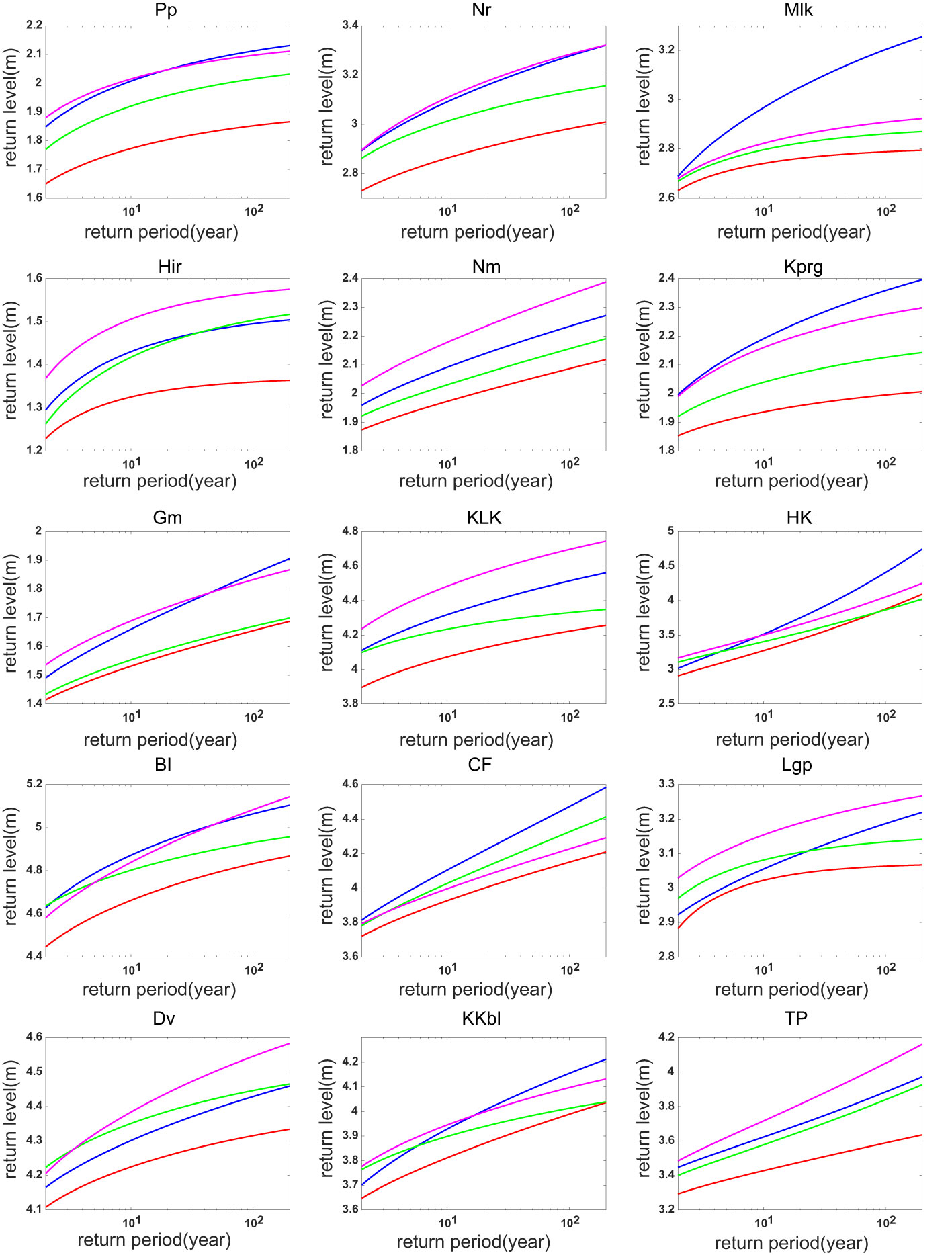
Figure 5 Return levels of the ESL at present (red line) and under the 2.0°C warming scenario: MIROC6 (blue line), CMCC-ESM2 (green line), EC-Earth3 (pink line).
To further quantify the potential influences of warming magnitudes on the return levels and return periods, we list in Table 4 the present and future 100-year return levels, as well as the future return periods of the present 100-year return level in the climate models under 1.5°C and 2°C warming scenarios. Compared with the historical observations in the past four decades, the return levels predicted by the three climate models mainly exhibit weak changes under the 1.5°C warming condition. Especially at Nr, Nm, Gm, CF, Lgp, and Dv stations, the changing amplitudes of 100-year return levels corresponding to 1.5°C warming are mostly less than 0.05 m. At other stations, however, the inter-model discrepancies are relatively larger. At Pp, Mlk, and HK stations, the increases of 100-year return levels predicted by MIROC6 are 0.16 m, 0.22 m, and 0.51 m, respectively, significantly higher than the predicted values in the other two models. At Hir, Kprg, KLK, and TP stations, EC-Earth3 predicts the 100-year return levels to increase by 0.11 m, 0.12 m, 0.28 m, and 0.17 m under the 1.5°C warming, which are also relatively higher than the increments in the other two models. In contrast, the CMCC-ESM2 predicts small differences between the present and the future return levels at most tide gauge sites. Such an inter-model diversity stems partly from the differences of climate models in simulating the SLP, which, as suggested by some recent studies, can be potentially attributed to the model biases in response to historical forcing (Ose et al., 2022; Wills et al., 2022). Compared with the other two models, CMCC-ESM2 simulates much weaker fluctuations of SLP, resulting in relatively weaker variability of the predicted ηCE, leading to smaller return levels.
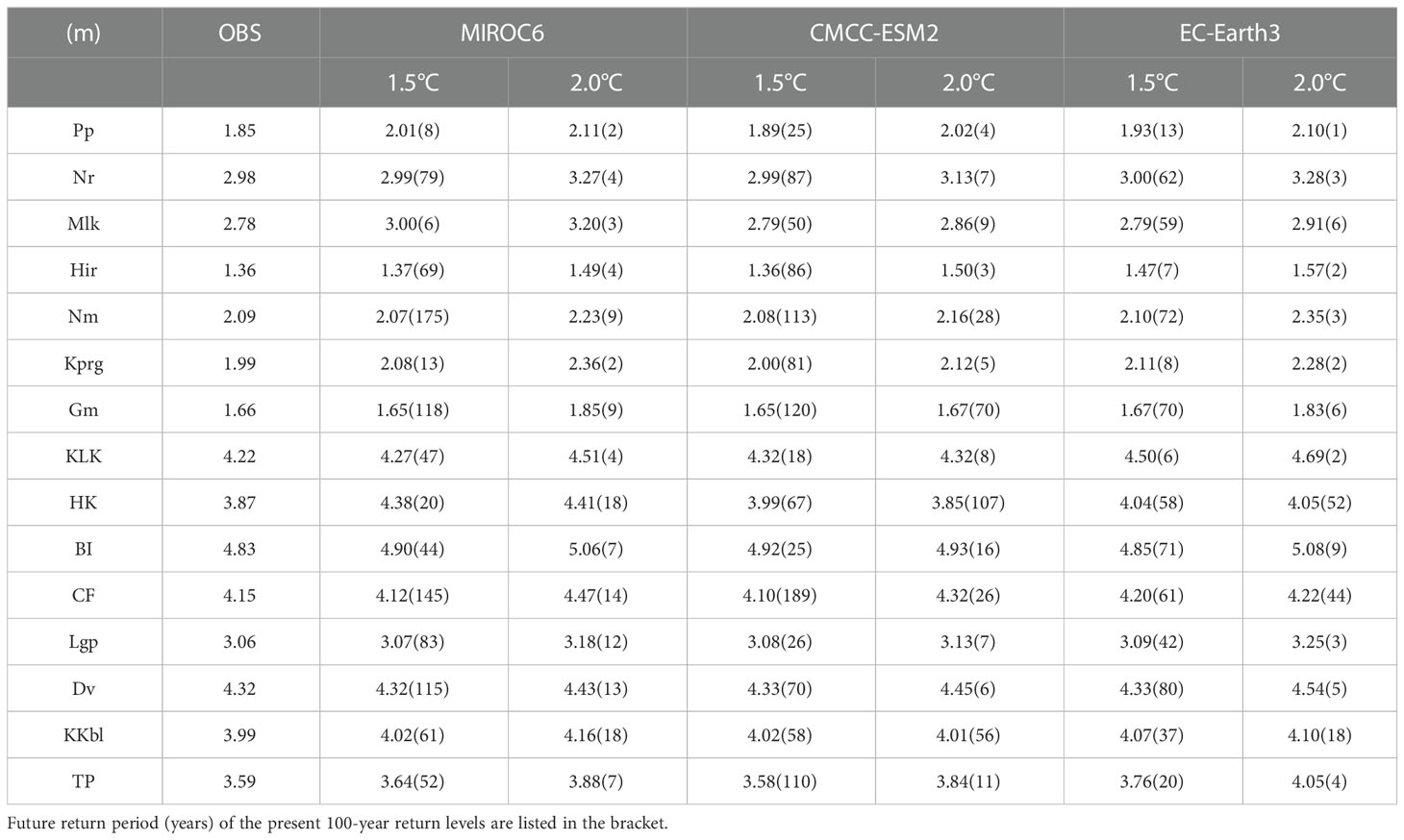
Table 4 Hundred-year return levels (m) of the ESL in the present day, and under the 1.5°C and 2.0°C warming scenarios at 15 tide gauges.
Despite the above-mentioned inter-model discrepancies, the results of the three climate models consistently suggest that the increments of 100-year return level are much larger under the warming scenario of 2°C than 1.5°C (Table 4). Compared with the values derived from tide gauge observations, the results of MIROC6 model suggest that the 100-year return levels under 2°C warming increase by 0.11~0.54 m at 15 tide gauge sites, which are about 0.03~0.35 m higher than the values under 1.5°C warming. The return period of the present 100-year return levels ranges from 2 to 18 years under 2°C warming. The CMCC-ESM2 simulations also show that at 14 tide gauge stations except for HK, the 100-year return levels increase by 0.01~0.25m from the present day to the 2°C warming scenario, and the return period of present 100-year return levels decreases to 3~56 years under 2°C warming. The corresponding changes from 1.5°C to 2°C of global warming are -0.01~0.26 m for 100-year return levels. For the HK station, as discussed above, the varying magnitude of SLP projected by CMCC-ESM2 is pretty large during 2018-2026 and becomes relatively smaller during 2026-2040, resulting in the predicted 100-year return level under 2°C warming being smaller than that under 1.5°C warming (3.85 m versus 3.99 m, see Table 4). The 100-year return levels based on the EC-Earth3 increase by 0.07-0.47m from the present day to the 2°C warming scenario. Compared with the 1.5°C warming condition, the 100-year return levels increase by 0.01-0.28m under 2°C warming. The corresponding return periods of the present 100-year return levels reduce to 1-52 years, significantly shorter than those under 1.5°C warming. The results of all three models suggest that an additional 0.5°C warming from 1.5°C to 2°C strongly impacts ESLs along the coasts and islands of the tropical western Pacific.
Contributions of different factors to the ESLs
This study also assessed the roles of mean sea level, tides, and water levels caused by extreme weather in determining the ESL at each tide gauge based on the historical data during 1980-2018 and the simulations of the EC-Earth3 model during 2019-2050. By selecting the respective values of these three components at the time of ESL occurrence, we evaluated the potential impacts of their time series on the long-term trend and interannual-to-decadal variability of ESL. Here we take the results of Nr and KLK stations as examples. As shown in Figure 6, the secular trends of ESLs and mean sea levels are almost the same for both Nr and KLK stations. The ESLs at the two stations rise at the rates of 5.29 mm/year and 11.6 mm/year, respectively. While the trends of mean sea levels are 5.45 mm/year and 8.20 mm/year, respectively. It indicates that mean sea level may play an important role in the long-term changes of ESLs. After removing the long-term trends, the correlation coefficients between ESL and the sum of water level caused by the tide and extreme weather are 0.848 for Nr and 0.969 for KLK, suggesting that the interannual-to-decadal variability of ESLs is also significantly influenced by water level fluctuations associated with the tide and extreme weather. When the high water level caused by extreme weather meets the high tide, a significant ESL event could probably be generated. Therefore, the influence of these two factors should be considered in more detail when analyzing specific ESL events. Besides, we also calculated the percentage of explained variance of mean sea level, tide, and extreme weather to ESL variability. For Nr station, mean sea level, extreme weather, and tide can explain 40.1%, 45.4%, and 14.5% of the variance, respectively. And mean sea level, extreme weather, and tide can explain 33.4%, 37.6%, and 29.0% of the variance, respectively, at KLK station. Similarly, the results from other stations or other climate models also consistently suggest that the long-term trends of ESL during 1980-2050 are mainly contributed by the yearly-mean sea level, while the contributions of extreme weather and tide are also crucial on the interannual-to-decadal timescales (see Table 5).
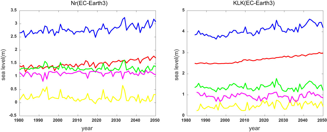
Figure 6 Comparison of ESL components at Nr and KLK stations: ESL (blue line), mean sea level (red line), sea level caused by tide plus extreme weather (green line), by tide (pink line) only, and by extreme weather (yellow line) only.
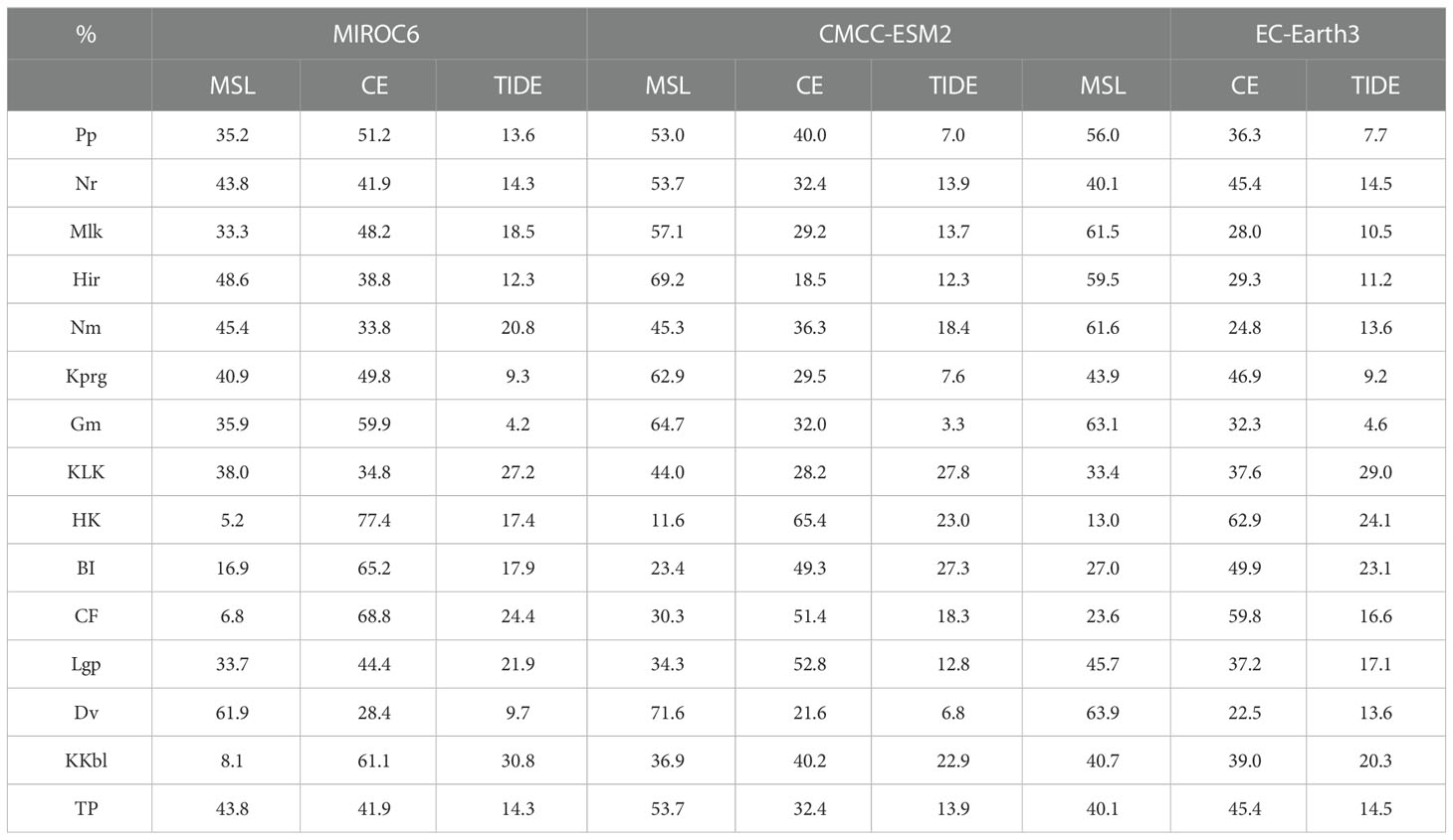
Table 5 The percentage of explained variance of mean sea level, extreme weather, and tide to the ESL variability based on three CMIP6 model simulations.
Conclusion and discussion
Using hourly sea level data from 15 tide gauges along the coasts and islands, the atmospheric forcing from ERA5 reanalysis, and three climate model simulations in CMIP6, this study analyzed the historical ESL variability over the tropical western Pacific and then further evaluated the future ESL changes in 1.5°C and 2°C warmer climates.
The ESL presents an overall rising trend from 1980-2018 over the tropical western Pacific. Meanwhile, the ESL trends derived from EEMD show different time-varying features at different tide gauges. At Hir and KLK, the growing trends are almost linear. At Nm, Gm, BI, and CF, the growing trends are not obvious initially but strengthen gradually. At Nr, Mlk, Kprg, HK, Lgp, and Dv, the growing trends weaken gradually. At Pp, KKbl, and TP, the ESLs show obvious rising trends before 2005 and then shift to decline afterward. The comparison between ESL and mean sea level suggests that the mean sea level essentially modulates the secular ESL trend and the interannual-to-decadal ESL variability during 1980-2018. The contribution of mean sea level to ESL appears more significant on small islands in the open ocean than on the coastlines of continents or within the SCS.
A sea level prediction model involving the influences of mean sea level, tides, and extreme weather events is established to assess the future ESL changes under different warming scenarios. The return levels of ESLs differ significantly under the 1.5°C and 2.0°C warming scenarios. Compared with the 1.5°C warming scenario, the return levels of ESL at most tide gauges along the coasts and islands of the tropical western Pacific show significant increases under 2.0°C warming scenario. It means that the additional 0.5°C warming will significantly increase the intensity and frequency of ESLs over the tropical western Pacific. Therefore, limiting anthropogenic warming to 1.5°C rather than 2.0°C, as the Paris Climate Agreement recommended, will provide key benefits for mitigating the flooding risks and damages on low-lying islands and coasts over the tropical western Pacific.
The combination of historical data and future estimations by the prediction model suggests that the secular increasing trends of ESL and mean sea level are almost the same in magnitude during 1980-2050, while the interannual-to-decadal ESL variability of ESL is also substantially influenced by tides and extreme weather events. The novelty of this study is that we detailedly show the similarities and differences of ESL changes at 15 tide gauge stations in the tropical western Pacific and illustrate the corresponding future ESL responses to the different warming scenarios of 1.5°C and 2°C. There are also some aspects that can be further studied. In this paper, we mainly use a multivariate linear regression method to simulate the value of ηCE at 15 tide gauge sites (Cayan et al., 2008). The advantage of this method is effective and convenient, which is more suitable for the analysis of individual stations. However, this method only depends on the linear relationship between SLP, wind stress, and ηCE, and does not consider the nonlinear interaction of tide, storm surges, and waves, which may lead to certain errors (Arns et al., 2015). In some previous works predicting global ESLs, the storm surge water level and significant wave height are derived from model simulations (Vousdoukas et al., 2018; Kirezci et al., 2020; Tebaldi et al., 2021). It is another feasible scheme to analyze the hourly simulation results directly. But it may also bring other uncertainty due to the simulation biases in climate models.
On the other hand, the results of this paper are mainly obtained by statistical analysis, and the underlying physical processes that affect ESL changes have not been well explained. So, future work will analyze the physical mechanisms of ESL changes in the tropical western Pacific. One of the research focuses can be the dynamic linkage between ESLs and climate variabilities, such as ENSO, PDO, and Atlantic Multidecadal Oscillation (AMO). Another potential research field is the impacts of the surge, which is the component of the water level largely driven by the wind. Some studies have taken the water level data from tide gauges minus the water level caused by the tide as a surge and analyzed the relationships amid tides, surges, their interactions, and ESLs (Haigh et al., 2013; Feng and Tsimplis, 2014; Wang and Zhou, 2017; Feng et al., 2018a). In recent years, the skew surge (defined as the difference between the maximum sea level occurring around high tide and the astronomical high‐tide level) has become a popular indicator for analyzing the correlation between ESL and surge (Marcos and Woodworth, 2017; Feng et al., 2019). But these research fields are still in the exploratory stage and have much room for improvement in the future.
Data availability statement
The original contributions presented in the study are included in the article/supplementary material. Further inquiries can be directed to the corresponding authors.
Author contributions
WZ and YD contributed to the conception and design of the study. YZ and WZ contributed to the methodology and modeling. YZ performed the dataset analyses, and visualization, with contributions from WZ. YZ prepared the manuscript draft. All authors were involved in the writing of the manuscript and discussed the results and the implications. All authors contributed to the article and approved the submitted version.
Funding
This research is funded by the National Key R&D Program of China (2019YFA0606702), the National Natural Science Foundation of China (91858202, 41776003), Southern Marine Science and Engineering Guangdong Laboratory (Guangzhou) (2019BT02H594), and Chinese Academy of Sciences (133244KYSB20190031, 183311KYSB20200015, SCSIO220201).
Acknowledgments
This study benefits from discussions with Drs. Yongxiang Huang and Lianyi Zhang.
Conflict of interest
The authors declare that the research was conducted in the absence of any commercial or financial relationships that could be construed as a potential conflict of interest.
Publisher’s note
All claims expressed in this article are solely those of the authors and do not necessarily represent those of their affiliated organizations, or those of the publisher, the editors and the reviewers. Any product that may be evaluated in this article, or claim that may be made by its manufacturer, is not guaranteed or endorsed by the publisher.
References
Arns A., Wahl T., Dangendorf S., Jensen J. (2015). The impact of sea level rise on storm surge water levels in the northern part of the German bight. Coast. Eng. 96, 118–131. doi: 10.1016/j.coastaleng.2014.12.002
Cayan D. R., Bromirski P. D., Hayhoe K., Tyree M., Dettinger M. D., Flick R. E. (2008). Climate change projections of sea level extremes along the California coast. Climatic Change 87 (S1), 57–73. doi: 10.1007/s10584-007-9376-7
Chen X., Zhang X., Church J. A., Watson C. S., King M. A., Monselesan D., et al. (2017). The increasing rate of global mean sea-level rise during 1993–2014. Nat. Climate Change 7 (7), 492–495. doi: 10.1038/nclimate3325
Dosio A., Mentaschi L., Fischer E. M., Wyser K. (2018). Extreme heat waves under 1.5 °C and 2 °C global warming. Environ. Res. Lett 13 (5), 054006. doi: 10.1088/1748-9326/aab827
Edwards T. L., Nowicki S., Marzeion B., Hock R., Goelzer H., Seroussi H., et al. (2021). Projected land ice contributions to twenty-first-century sea level rise. Nature 593 (7857), 74–82. doi: 10.1038/s41586-021-03302-y
Ezer T., Dangendorf S. (2020). Global sea level reconstruction for 1900–2015 reveals regional variability in ocean dynamics and an unprecedented long weakening in the gulf stream flow since the 1990s. Ocean Sci. 16 (4), 997–1016. doi: 10.5194/os-16-997-2020
Feng J., Jiang W. (2015). Extreme water level analysis at three stations on the coast of the northwestern pacific ocean. Ocean Dyn. 65 (11), 1383–1397. doi: 10.1007/s10236-015-0881-3
Feng J., Li H., Li D., Liu Q., Wang H., Liu K., et al. (2018b). Changes of extreme Sea level in 1.5 and 2.0°C warmer climate along the coast of China. Front. Earth Sci. 6. doi: 10.3389/feart.2018.00216
Feng J., Li D., Wang T., Liu Q., Deng L., Zhao L., et al. (2019). Acceleration of the extreme Sea level rise along the Chinese coast. Earth Space Sci. 6 (10), 1942–1956. doi: 10.1029/2019ea000653
Feng J., Li D., Wang H., Liu Q., Zhang J., Li Y., et al. (2018a). Analysis on the extreme Sea levels changes along the coastline of bohai Sea, China. Atmosphere 9 (8), 324. doi: 10.3390/atmos9080324
Feng X., Tsimplis M. N. (2014). Sea Level extremes at the coasts of China. J. Geophys. Res.: Oceans 119 (3), 1593–1608. doi: 10.1002/2013jc009607
Feng J., von Storch H., Jiang W., Weisse R. (2015). Assessing changes in extreme sea levels along the coast of China. J. Geophys. Res.: Oceans 120 (12), 8039–8051. doi: 10.1002/2015jc011336
Haigh I. D., Wijeratne E. M. S., MacPherson L. R., Pattiaratchi C. B., Mason M. S., George S. (2013). Estimating present day extreme water level exceedance probabilities around the coastline of Australia: tides, extra-tropical storm surges and mean sea level. Clim. Dyn. 42 (1-2), 121–138. doi: 10.1007/s00382-012-1652-1
Huang N. E., Shen Z., Long S. R. (1999). A new view of nonlinear water waves: the Hilbert spectrum. Annu. Rev. Fluid Mech. 31, 417–457. doi: 10.1146/annurev.fluid.31.1.417
Huang N. E., Shen Z., Long S. R., Wu M. C., Shih E. H., Zheng Q., et al. (1998). The empirical mode decomposition and the Hilbert spectrum for nonstationary time series analysis. Proc. R. Soc. London 454, 903–995. doi: 10.1098/rspa.1998.0193
Huang W., Xu S., Nnaji S. (2008). Evaluation of GEV model for frequency analysis of annual maximum water levels in the coast of united states. Ocean Eng. 35, 1132–1147. doi: 10.1016/j.oceaneng.2008.04.010
Jevrejeva S., Grinsted A., Moore J. C., Holgate S. (2006). Nonlinear trends and multiyear cycles in sea level records. J. Geophys. Res. 111 (C9), C09012. doi: 10.1029/2005jc003229
Kirezci E., Young I. R., Ranasinghe R., Muis S., Nicholls R. J., Lincke D., et al. (2020). Projections of global-scale extreme sea levels and resulting episodic coastal flooding over the 21st century. Sci. Rep. 10 (1), 11629. doi: 10.1038/s41598-020-67736-6
Lehner F., Coats S., Stocker T. F., Pendergrass A. G., Sanderson B. M., Raible C. C., et al. (2017). Projected drought risk in 1.5°C and 2°C warmer climates. Geophys. Res. Lett. 44 (14), 7419–7428. doi: 10.1002/2017gl074117
Lyard F. H., Allain D. J., Cancet M., Carrère L., Picot N. (2021). FES2014 global ocean tide atlas: design and performance. Ocean Sci. 17, 615–649. doi: 10.5194/os-17-615-2021
Marcos M., Calafat F. M., Berihuete Á., Dangendorf S. (2015). Long-term variations in global sea level extremes. J. Geophys. Res.: Oceans 120 (12), 8115–8134. doi: 10.1002/2015jc011173
Marcos M., Tsimplis M. N., Shaw A. G. P. (2009). Sea Level extremes in southern Europe. J. Geophys. Res. 114 (C1), C01007. doi: 10.1029/2008jc004912
Marcos M., Woodworth P. L. (2017). Spatiotemporal changes in extreme sea levels along the coasts of the north Atlantic and the gulf of Mexico. J. Geophys. Res.: Oceans 122 (9), 7031–7048. doi: 10.1002/2017jc013065
Marzeion B., Hock R., Anderson B., Bliss A., Champollion N., Fujita K., et al. (2020). Partitioning the uncertainty of ensemble projections of global glacier mass change. Earth’s Future 8 (7), e2019EF001470. doi: 10.1029/2019ef001470
Menéndez M., Woodworth P. L. (2010). Changes in extreme high water levels based on a quasi-global tide-gauge data set. J. Geophys. Res.: Oceans 115 (C10), C10011. doi: 10.1029/2009jc005997
Mentaschi L., Vousdoukas M., Voukouvalas E., Sartini L., Feyen L., Besio G., et al. (2016). The transformed-stationary approach: a generic and simplified methodology for non-stationary extreme value analysis. Hydrol. Earth Syst. Sci. 20 (9), 3527–3547. doi: 10.5194/hess-20-3527-2016
Muis S., Verlaan M., Nicholls R. J., Brown S., Hinkel J., Lincke D., et al. (2017). A comparison of two global datasets of extreme sea levels and resulting flood exposure. Earth’s Future 5 (4), 379–392. doi: 10.1002/2016ef000430
Mulet S., Rio M.-H., Etienne H., Artana C., Cancet M., Dibarboure G., et al. (2021). The new CNES-CLS18 global mean dynamic topography. Ocean Sci. 17 (3), 789–808. doi: 10.5194/os-17-789-2021
Ose T., Endo H., Takaya Y., Maeda S., Nakaegawa T. (2022). Robust and uncertain sea-level pressure patterns over summertime East Asia in the CMIP6 multi-model future projections. J. Meteorol. Soc. Japan 100, 631–645. doi: 10.2151/jmsj.2022-032
Rasmussen D. J., Bittermann K., Buchanan M. K., Kulp S., Strauss B. H., Kopp R. E., et al. (2018). Extreme sea level implications of 1.5 °C, 2.0 °C, and 2.5 °C temperature stabilization targets in the 21st and 22nd centuries. Environ. Res. Lett. 13 (3), 034040. doi: 10.1088/1748-9326/aaac87
Slangen A. B. A., Carson M., Katsman C. A., van de Wal R. S. W., Köhl A., Vermeersen L. L. A., et al. (2014). Projecting twenty-first century regional sea-level changes. Clim. Change 124 (1-2), 317–332. doi: 10.1007/s10584-014-1080-9
Takbash A., Young I. (2020). Long-term and seasonal trends in global wave height extremes derived from ERA-5 reanalysis data. J. Mar. Sci. Eng. 8 (12), 1015. doi: 10.3390/jmse8121015
Tebaldi C., Ranasinghe R., Vousdoukas M., Rasmussen D. J., Vega-Westhoff B., Kirezci E., et al. (2021). Extreme sea levels at different global warming levels. Nat. Clim. Chang. 11 (9), 746–751. doi: 10.1038/s41558-021-01127-1
UNFCCC. (2015a). Report of the conference ofthe parties on its twenty-first session, held in Paris from 30November–13December 2015 (New York: United Nations).
UNFCCC. (2015b). Report on the structured ExpertDialogue on the 2013-2015 review (New York: United Nations).
Vousdoukas M. I., Mentaschi L., Voukouvalas E., Verlaan M., Jevrejeva S., Jackson L. P., et al. (2018). Global probabilistic projections of extreme sea levels show intensification of coastal flood hazard. Nat. Commun. 9 (1), 2360. doi: 10.1038/s41467-018-04692-w
Wada Y., van Beek L. P. H., Sperna Weiland F. C., Chao B. F., Wu Y.-H., Bierkens M. F. P. (2012). Past and future contribution of global groundwater depletion to sea-level rise. Geophys. Res. Lett. 39 (9), n/a–n/a. doi: 10.1029/2012gl051230
Wahl T., Haigh I. D., Nicholls R. J., Arns A., Dangendorf S., Hinkel J., et al. (2017). Understanding extreme sea levels for broad-scale coastal impact and adaptation analysis. Nat. Commun. 8, 16075. doi: 10.1038/ncomms16075
Wang W., Zhou W. (2017). Statistical modeling and trend detection of extreme sea level records in the pearl river estuary. Adv. Atmos. Sci. 34 (3), 383–396. doi: 10.1007/s00376-016-6041-y
Weisse R., Bellafiore D., Menendez M., Mendez F., Nicholls R. J., Umgiesser G., et al. (2014). Changing extreme sea levels along European coasts. Coast. Eng. 87, 4–14. doi: 10.1016/j.coastaleng.2013.10.017
Wills R. C. J., Dong Y., Proistosecu C., Armour K. C., Battisti D.S. (2022). Systematic climate model biases in the large-scale patterns of recent sea-surface temperature and sea-level pressure change. Geophys. Res. Lett. 49, e2022GL100011. doi: 10.1029/2022GL100011
Keywords: extreme sea level, tropical western Pacific, return level, return period, future projection
Citation: Zheng Y, Zhuang W and Du Y (2023) Extreme sea level changes over the tropical western Pacific in 1.5 °C and 2.0 °C warmer climates. Front. Mar. Sci. 10:1130769. doi: 10.3389/fmars.2023.1130769
Received: 23 December 2022; Accepted: 27 February 2023;
Published: 14 March 2023.
Edited by:
Şükrü Beşiktepe, Dokuz Eylül University, TürkiyeReviewed by:
Yun Qiu, State Oceanic Administration, ChinaWenfang Lu, Sun Yat-sen University, China
Kai Yu, Hohai University, China
Copyright © 2023 Zheng, Zhuang and Du. This is an open-access article distributed under the terms of the Creative Commons Attribution License (CC BY). The use, distribution or reproduction in other forums is permitted, provided the original author(s) and the copyright owner(s) are credited and that the original publication in this journal is cited, in accordance with accepted academic practice. No use, distribution or reproduction is permitted which does not comply with these terms.
*Correspondence: Wei Zhuang, d3podWFuZ0B4bXUuZWR1LmNu; Yan Du, ZHV5YW5Ac2NzaW8uYWMuY24=