
95% of researchers rate our articles as excellent or good
Learn more about the work of our research integrity team to safeguard the quality of each article we publish.
Find out more
ORIGINAL RESEARCH article
Front. Mar. Sci. , 20 July 2023
Sec. Ocean Observation
Volume 10 - 2023 | https://doi.org/10.3389/fmars.2023.1129876
This article is part of the Research Topic Colour and Light in the Ocean, volume II View all 27 articles
 Martin Hieronymi1*
 Shun Bi1
 Dagmar Müller2
 Eike M. Schütt1,3
 Daniel Behr1
 Carsten Brockmann2Carole Lebreton2
 François Steinmetz4Kerstin Stelzer2Quinten Vanhellemont5
Satellite remote sensing allows large-scale global observations of aquatic ecosystems and matter fluxes from the source through rivers and lakes to coasts, marginal seas into the open ocean. Fuzzy logic classification of optical water types (OWT) is increasingly used to optimally determine water properties and enable seamless transitions between water types. However, effective exploitation of this method requires a successful atmospheric correction (AC) over the entire spectral range, i.e., the upstream AC is suitable for each water type and always delivers classifiable remote-sensing reflectances. In this study, we compare five different AC methods for Sentinel-3/OLCI ocean color imagery, namely IPF, C2RCC, A4O, POLYMER, and ACOLITE-DSF (all in the 2022 current version). We evaluate their results, i.e., remote-sensing reflectance, in terms of spatial exploitability, individual flagging, spectral plausibility compared to in situ data, and OWT classifiability with four different classification schemes. Especially the results of A4O show that it is beneficial if the performance spectrum of the atmospheric correction is tailored to an OWT system and vice versa. The study gives hints on how to improve AC performance, e.g., with respect to homogeneity and flagging, but also how an OWT classification system should be designed for global deployment.
Ocean Color (OC) has been identified as an Essential Climate Variable (ECV), because of its capability to observe various aspects of the marine environment synoptically at global scales (GCOS, 2011; Hollmann et al., 2013). The color of the ocean is determined by absorption and scattering interactions of sunlight with water, free-floating particles and dissolved substances in the upper water layer (current state of research on this is summarized by Bi et al., 2023). Color, or more specifically the remote-sensing reflectance, Rrs, is defined as the spectral (back-scattered) water-leaving radiance, Lw, in proportion to the total down-welling plane irradiance, Ed. The reference point lies directly above the sea surface at the bottom-of-atmosphere (BOA). The spectral range of Rrs includes not only the visible (VIS) range, which is perceived as color often defined for wavelengths from 380 to 760 nm, but also parts of the ultraviolet (UV) and near-infrared (NIR) spectral range; it is primarily determined by the pure water absorption (e.g., Bi et al., 2023). Space-borne ocean color sensors, however, measure spectral radiances, LTOA, at the top-of-atmosphere (TOA) from the given viewing direction. This signal is strongly influenced by light interactions in the atmosphere, like scattering by air molecules, and aerosols or absorption by atmospheric gases, but also by light reflections at the sea surface (e.g., IOCCG, 2010; Frouin et al., 2019). Moreover, whitecaps and air bubbles in water, not related to the actual ocean color, contribute to the water-leaving signal (e.g., Dierssen, 2019). The process of retrieving unobstructed remote-sensing reflectance at surface level from TOA radiance is typically referred to as atmospheric correction (AC).
Spectral remote-sensing reflectance is the fundamental parameter from which biogeo-optical properties and corresponding concentrations of optically active water constituents can be derived. The concentration of the pigment chlorophyll-a in water, Chl, is widely used as a proxy for the phytoplankton biomass in the upper water layer; Chl is also considered as an ECV as it is linked to the marine carbon-cycle. The Global Climate Observing System (GCOS, 2011) defines a target accuracy requirement for Rrs (strictly speaking for the water-leaving radiance) of 5% specifically for the blue and green wavelengths and 30% for Chl. This applies to so-called Case-1 (C1) waters whose inherent optical properties (IOPs) primarily depend on phytoplankton, its abundance and its degradation products; this is generally the case for open oceans. In contrast, all “optically complex” waters of marginal seas, coastal and inland water bodies are summarized as Case-2 (C2) where additional water constituents such as non-algal particles (NAP) and colored dissolved organic matter (CDOM) considerably influence the water color (Morel and Prieur, 1977; Bi et al., 2023). CDOM is primarily leached from decaying detritus and terrestrial organic matter, but it can also be yielded from precipitation with elevated CDOM levels in continentally influenced rainwater (Kieber et al., 2006). The accepted uncertainties of Rrs and subsequent ocean color products are considerably higher for Case-2 waters and GCOS recommends the implementation of specifically tailored algorithms. Based on this rationale, EUMETSAT for example offers two independent Chl products (based on different AC methods) from the operational Ocean and Land Color Instrument (OLCI) on board the Sentinel-3 satellites, namely CHL_OC4ME for Case-1 and CHL_NN for Case-2 waters. User consultations, however, reveal a clear priority for ocean color algorithms that work across C1-C2 waters, or at least that demarcate the boundary between the two; moreover, appropriate and steady ocean color products are required for climate change studies (Sathyendranath et al., 2017).
The usage of branching and blending of specialized algorithms for seamless transition and case-optimized phytoplankton estimates has increased over the course of the recent years. Smith et al. (2018) and Kajiyama et al. (2018) for example have developed OLCI-specific bipartite switching algorithms for regionally optimized Chl retrievals. More holistic approaches involve a pre-classification of Rrs spectra into several optical water types (OWT) in order to display the full spectral diversity of oceanic, coastal, and inland waters (e.g., Moore et al., 2001; Martin Traykovski and Sosik, 2003; Vantrepotte et al., 2012; Shi et al., 2013; Moore et al., 2014; Mélin and Vantrepotte, 2015; Minu et al., 2016; Eleveld et al., 2017; Hieronymi et al., 2017; Jackson et al., 2017; Spyrakos et al., 2018; Soomets et al., 2019; Uudeberg et al., 2020; Jia et al., 2021; Wei et al., 2022). However, effective exploitation of this method presumes a successful atmospheric correction over the entire spectral range. Residual errors from imperfect atmospheric correction, which are not reproducible by combination of mean OWT reflectance spectra, can result in very low total memberships and therefore, prove the unfitness of the processing constellation for this case. This leads to the need that the upstream AC method is within the scope for each water type and that it delivers always-sufficient total memberships.
There are various sensor-specific AC methods, which supply remote-sensing reflectance mostly optimized for either oceanic, coastal or inland waters, e.g., described in IOCCG (2010) or Frouin et al. (2019). The corresponding AC performance can differ significantly depending on the selected evaluation data, optical water types, applied flagging, sensor properties like camera boundaries, the presence of transparent clouds or sun glint (e.g., Goyens et al., 2013; Müller et al., 2015a; Müller et al., 2015b; Qin et al., 2017; Tilstone et al., 2017; Mograne et al., 2019). Frouin et al. (2019) listed a number of significant issues for atmospheric correction including clouds, adjacency effects, whitecaps, the Earth atmosphere’s curvature, multiple scattering, and polarization. Moreover, atmospheric corrections have serious difficulties in cases with high CDOM or NAP concentrations in water, i.e., very dark or bright, so called extreme Case-2 waters (Hieronymi et al., 2016; Hieronymi et al., 2017). Absorption of dissolved organic matter causes an exponential reduction of the reflectance especially in the blue; this is from a TOA-reflectance point of view, a comparable spectral effect as Rayleigh scattering by air molecules and hence ambiguous. Absorbing or extremely absorbing Case-2 waters (C2A, C2AX) are characterized by low spectral Rrs with maximum in the green and in cases with very high CDOM-content (i.e., aCDOM(440) >1 m-1) in the yellow, red, or even NIR spectral range. Particles in water absorb, but above all also scatter light, which leads to increased reflectance at higher concentrations, partly also in the NIR. The spectral absorption and much higher scattering of non-algae particles also have an approximately exponential course, as does the Rayleigh influence. At relatively high NAP concentrations of 1 g m-3, one speaks of scattering Case-2 waters (C2S); at NAP > 100 g m-3 of extremely scattering waters (C2SX) respectively. Furthermore, AC problems arise in the presence of very high concentrations of phytoplankton and floating scum with non-negligible NIR reflectance (e.g., Reinart and Kutser, 2006). Clearly, a combination of different AC algorithms can potentially improve an all-water-type-embracing Rrs-retrieval; examples are given in Shi and Wang (2009); Aurin et al. (2013); Bi et al. (2018); Liu et al. (2019), and Schroeder et al. (2022). However, programmatic linking of fundamentally different AC algorithms can be challenging and switching may lead to spatial inconsistency or artefacts in the retrievals.
Several AC methods exist for ocean color imagery of Sentinel-3/OLCI. However, their range of validity is not always clear and they do not always fulfil all requirements for unlimited usability of OWT-based water algorithms like the ONNS algorithm by Hieronymi et al. (2017). In this study, we compare five conceptually different atmospheric correction methods for Sentinel-3/OLCI (specified in Table 1): 1) the standard (baseline) Level-2 AC – Instrument Processing Facility (IPF), 2) the alternative Level-2 AC C2RCC, 3) a novel atmospheric correction for diverse optical water types (A4O) by Hieronymi et al. (in prep.), 4) POLYMER by Steinmetz et al. (2011), and 5) the Dark Spectrum Fitting (DSF) implemented in ACOLITE by Vanhellemont and Ruddick (2021). There are also other methods available that can be applied to OLCI (e.g., Guanter et al., 2010; Gossn et al., 2019; Schroeder et al., 2022), but we focus on these five ACs as representative examples of diverse approaches. Based on optically diverse Sentinel-3/OLCI images, we compare the capacity for data exploitation, the spatial plausibility and homogeneity (noise), and analyze the AC output, namely Rrs, in view of different OWT classification schemes. Moreover, we show comparisons with in situ match-up data. We are thereby attempting to demarcate the scope of application for each AC method and identify potentials for future improvements.
Table 1 Examined atmospheric correction methods for Sentinel-3/OLCI ocean color processing with AC-specific masking (plus INVALID and LAND for all).
The European Space Agency (ESA), together with the European Organisation for the Exploitation of Meteorological Satellites (EUMETSAT), operates the Sentinel series of satellites from the European Union Copernicus Programme. EUMETSAT provides Level-2 (L2) standard water products for Sentinel-3/OLCI. Our work refers to data of the ocean color “baseline atmospheric correction” from the Instrument Processing Facility (IPF), which has been operational since 2021 (OLCI Collection-3). The reflectances provided are the basis for the estimation of the chlorophyll-a concentration in Case-1 water, CHL_OC4ME. The AC was developed for the open ocean and is based on work of Gordon and Wang (1994); further developments of this method were summarized by Gordon (2021). Significant further developments regarding MERIS and OLCI are based on Antoine and Morel (1998), and Antoine and Morel (1999); Moore et al. (1999), and Nobileau and Antoine (2005). Major updates of IPF have been introduced in the Sentinel-3/OLCI L2 report for baseline collection (EUMETSAT, 2021); the report includes several comparisons with in situ data and reference missions, and lists the recommended flags. Particularly noteworthy is the recently implemented revision of the so-called bright pixel correction within the AC, which is applied everywhere, but brings improvements especially in NAP-dominated coastal waters.
The OLCI L2 processing includes a second “alternative” AC whose results are not provided, but they form the basis for the L2 Case-2 water products like chlorophyll-a concentration, CHL_NN. The AC uses neural networks (NN) for the retrieval of Rrs and also goes back to the MERIS heritage with works of Doerffer and Schiller (2007). The original Case-2 Regional (C2R) algorithm, which contains AC and water algorithms, was optimized for coastal waters of the North Sea. The algorithm was further developed in the CoastColour project (ESA) and is now known as C2RCC (Brockmann et al., 2016). C2RCC is available in the Sentinel Toolbox (SNAP). The neural networks used in the OLCI L2 processing and those of C2RCC are identical. However, there are small differences between OLCI operational NN products and outputs from the SNAP C2RCC processing due to some different pre-processing steps. In this study, the IPF-derived SVC gains (from Collection 3) are used for C2RCC processing directly on OLCI L1B data, which is done slightly different in the OLCI L2 ground segment NN processing (EUMETSAT, 2021). The application of sensor-specific and AC-specific system vicarious calibration (SVC) gains may have the biggest impact also in comparison with previous studies; in some studies, such as Cazzaniga et al. (2023), the same SVC gains are applied, in earlier studies than 2021, other SVC gains were used in some cases (e.g., Giannini et al., 2021). The pixel identification tool IdePix was used for cloud detection and corresponding additional flagging (Brockmann et al., 2013). Against usual recommendations to use equal processing levels for match-up analysis, the non-normalized Rrs product of C2RCC is used, which has a broader spectral range in the NIR necessary for some OWT models.
In the course of the last few years, Hieronymi et al. (in prep.) developed a novel atmospheric correction for diverse optical water types (A4O). The basis was C2RCC, but with fundamental conceptual revision to optimize classifiability with the OWT framework implemented in the OLCI Neural Network Swarm (ONNS) water algorithm (Hieronymi et al., 2017). The aim of A4O is to be applicable to all natural waters, from Case-1 to extremely scattering or absorbing Case-2 waters. Special attention was dedicated to phytoplankton diversity. A4O applies an ensemble of different neural networks and provides fully normalized Rrs. In addition, there are other differences to C2RCC; these include the specification of water temperature and salinity using global climatological data, the treatment of ocean whitecaps, the expansion of features in the NN training data, flagging, and an option for spectral and spatial smoothing of the signal. The IPF-SVC gains are also taken into account here primarily to compensate for sensor-specific differences, i.e., the instruments on Sentinel-3A and -3B. The invalid pixel expression refers primarily to an own cloud masking, all visible water areas are valid in principle (non-physical negative reflectance is never delivered). However, there are a number of warning flags, e.g., for pixels with possible land influence or strong sun glint signal, where results might be faulty. It is planned to publish A4O and ONNS in SNAP in the medium term.
POLYMER is an AC algorithm originally developed for oceanic and coastal waters (Steinmetz et al., 2011; Steinmetz and Ramon, 2018). It uses a spectral fitting scheme that relies on two models: a polynomial-like model of atmospheric reflectance and a model of water reflectance. It was developed primarily for correcting sun-glint contamination on images of the MERIS sensor, and has then been applied to several multispectral and hyperspectral sensors including OLCI. In addition to sun glint correction, it is also robust to aerosol contamination and other atmospheric and surface effects such as thin clouds and adjacency effects (Steinmetz and Ramon, 2018; Zhang et al., 2019). POLYMER is the only method in this study that does not use the IPF-SVC gains because all bands are used simultaneously for atmospheric correction. Thus, specific gains are used, generated by a dedicated spectrally coupled SVC scheme.
The Dark Spectrum Fitting (DSF) algorithm as implemented in ACOLITE, was originally developed for aquatic applications of satellite data with high spatial resolution in the meter to decameter scale, e.g., the Landsat series, Sentinel-2/MSI, Pléiades, and PlanetScope (Vanhellemont and Ruddick, 2018; Vanhellemont, 2019a; Vanhellemont, 2019b; Vanhellemont, 2020). Vanhellemont and Ruddick (2021) adapted the AC for Sentinel-3/OLCI especially for mapping of suspended particulate matter and chlorophyll-a concentration in turbid coastal waters. Thus, the main scope of ACOLITE-DSF is for aquatic applications for inland and coastal waters, but it can also be used over clearer waters and even land. The gains from IPF-SVC are also being considered here.
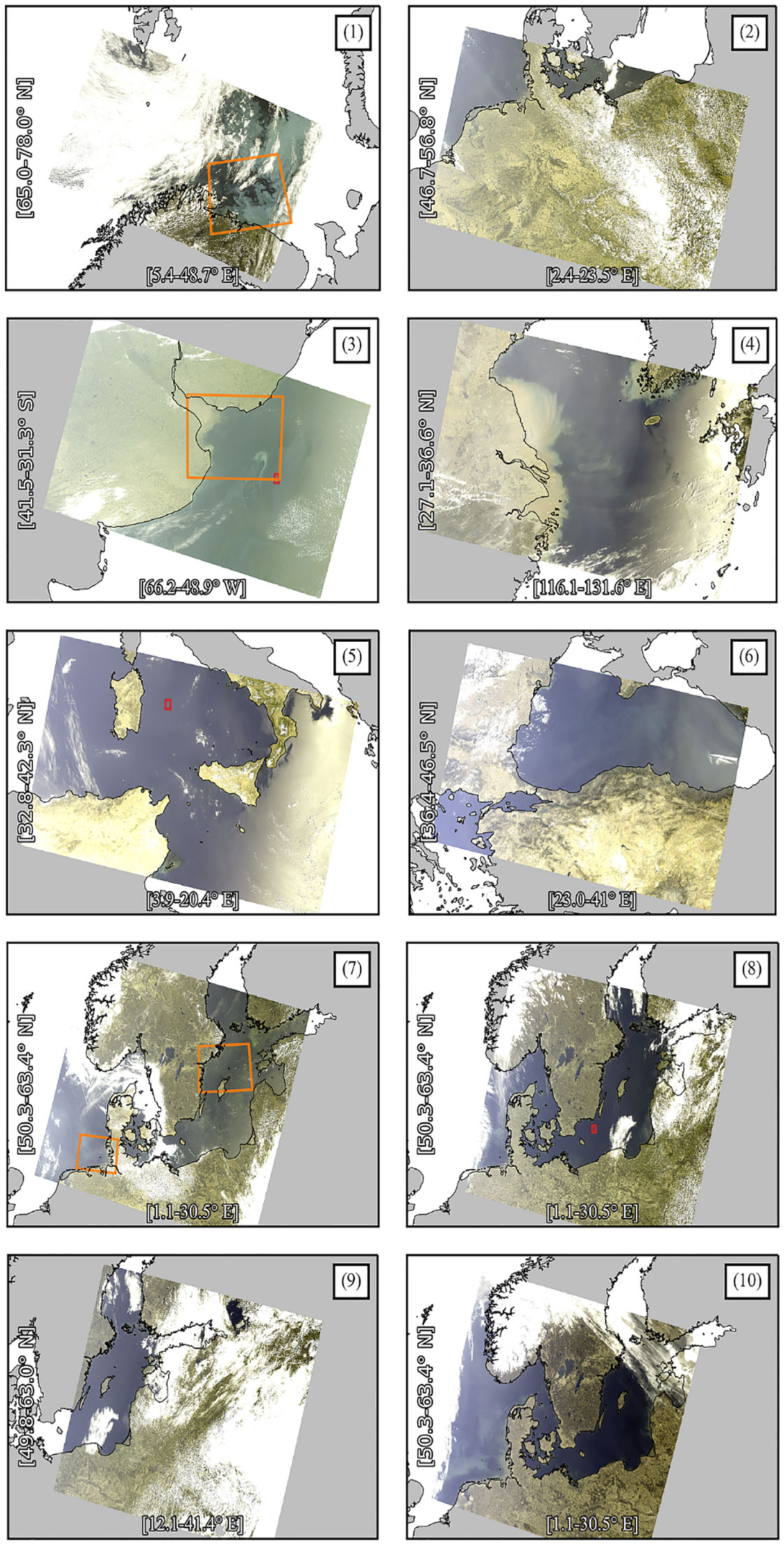
Ten full-resolution OLCI (Level-1) scenes were selected for analysis of the spatial AC performance (pixel size 300 m at nadir, swath width approximately 1270 km). They cover a wide variety of optical water types, regions, sun elevations, and sensor-viewing angles relative to the sun (Table 2; Appendix Figure A1). Approximately 47% of the observed Earth surface in the images is covered by water. Of these water areas, 36% are flagged for cloud-risk and 9% for sun-glint according to the A4O designation. For a representative analysis of these scenes, common masks were used where all 5x5 pixels around a central pixel must be valid. This is to eliminate possible cloud artefacts, cloud shadows, sun glint, and land adjacency effects as much as possible. The freely visible and in principle unrestricted water areas were visually checked. However, many of these water pixels are masked by the individual AC methods; especially IPF masks large areas because it produces negative Rrs values here. The selected free water areas cover 31.5 million pixels. Inland waters account for 4%. About 0.6% of the pixels show a characteristic red edge increase of TOA reflectance caused by floating biomass at the sea surface and are labelled as FLOATING in A4O. Hieronymi et al. (2016) suggested a definition for extremely scattering waters with Rrs(865) ≥ 0.005 sr-1; thus, the coverage of bright pixels depends on the AC method and is up to 4%.
Table 2 Selected test scenes with large cloud-free areas that cover high optical diversity (shown in Appendix Figure A1).
Independent validation was carried out for match-ups between OLCI imagery and AERONET-OC in situ measurement data (Zibordi et al., 2009) from 2016 to 2020 distributed through the ESA OC-CCI in situ database (Valente et al., 2022). The data set was limited to OLCI bands (± 2 nm). All Rrs measurements are normalized following Park and Ruddick (2005). The stations are widely distributed geographically, but often near coasts or in inland waters (GLO – Gloria, Black Sea; GDT – Gustav Dalen Tower, Baltic Sea; HLH – Helsinki Lighthouse, Baltic Sea; LIS – LISCO, Long Island Sound; LUC – Lucinda, East Coast of Australia; MVC – MVCO, US East Coast; PAL – Palgrunden, Lake in Sweden; VEN – Venice, Adriatic Sea; WAV – Wavecis_site_csi_6, Gulf of Mexico). Therefore, the water types are very similar and the data are not representative of the full range of all natural waters. In the cases where the entire spectra are available, the maximum reflectance lies at 560 nm in 89% cases of the data, only 11% have the maximum at 490 or 510 nm; there is no in situ data included with the maximum in blue bands<490 nm or at bands >560 nm. The vast majority of the data counts as Case-2 water. For band-wise comparisons, however, data from Case-1 waters are also included. Some of the AERONET-OC data from the Baltic Sea and the Black Sea represent distinct blooms of cyanobacteria or coccolithophores (e.g., Cazzaniga et al., 2021; Zibordi et al., 2022; Cazzaniga et al., 2023). However, for a comparison of AC results at all 16 (out of 21) OLCI bands, in situ data are often missing, especially in red and NIR bands. In general, band-shifting methods can be used to derive OLCI spectra from different band configurations, and the mean percentage retrieval error in the spectral range between 400 and 600 nm is usually less than 5%, but for red and NIR bands the uncertainties are much larger (Hieronymi, 2019). For this reason, additional band shifting was not used in this work, since the main purpose of the match-up comparison is to show the spectral plausibility of the AC results.
In order to be able to rudimentary quantify the spatial scenes in the transition from coastal water types and also to contextualize very turbid waters that are not covered in AERONET-OC, exemplary further in situ measurement data are considered. Firstly, reflectance measured by Hieronymi et al. in the North Sea/German Bight (OLCI match-up with scene #2) with a protocol described in Tilstone et al. (2020) and normalized with Park and Ruddick (2005). Secondly, OLCI match-ups with the PANTHYR system (Vansteenwegen et al., 2019) that is located in turbid coastal waters in Belgium. The data are provided by Vanhellemont and Ruddick (2021); ACOLITE-DSF was specially designed for these waters and a comparison with the AC candidates (albeit in different versions for ACOLITE-DSF, IPF, and C2RCC, but without A4O) was discussed in their original paper. Approximately half of the PANTHYR data are considered as extremely scattering waters using the above-mentioned definition, the other are C2S.
The Calvalus system (Fomferra et al., 2012) was used to identify OLCI image matches with in situ data within three hours of the satellite overpass. Altogether, there are 2545 match-ups between 2016 and 2020 for the nine AERONET-OC stations and 62 for PANTHYR (2019-2020) for OLCI-A & B. For some stations, there are only a few spectral bands for the comparison and the match-up number varies for each AC according to the filtering of valid data points. Duplicated-flagged values are not used. Mini-scenes of about 10x10 pixels in size were selected at IPF, C2RCC, and A4O, and 5x5 macro-pixels were extracted from them. In the case of POLYMER and ACOLITE-DSF, the complete scenes were processed first and the macro-pixels extracted from them. ACOLITE-DSF can be rather sensitive to size of the scene or sub-scene, and it is usually recommended to use a spatially limited study area with a single aerosol retrieval. For larger scenes, as used here, the aerosol retrieval is tiled and interpolated to the full extent. Individual tile contents may skew the results between tile centers.
The aggregation of the 5x5 macro-pixel follows mostly the procedure described in Müller et al. (2015a). The valid pixel expressions of each AC (Table 1) are applied; all valid pixels are screened for outliers per band using a threshold of 2.5 standard deviations. From the remaining valid pixels their mean value, μ, and standard deviation, σ, is calculated and the number of valid observations (excluding the outliers) is recorded. Based on the percentage coefficient of variation, CV, a match-up is considered in further analysis, if the spatial homogeneity is high for the particular band and therefore CV = σ/μ × 100% < 15%. Second, at least half of the pixels in the macro-pixel must be valid. These criteria are checked for each data point and band independently, so that AC solutions with some noise in a part of the spectral range may lose good match-ups here but retain part of the spectrum in other spectral regions. The number of match-ups will therefore vary per band, which allows some interpretation in terms of spatial noise.
To compare the performance of the AC methods, we use the match-up statistics recommended by EUMETSAT (2022). Besides the well-known linear regression statistics with the correlation coefficient (r), we use the root-mean-square-error (RMSE), median absolute deviation (mdAD), median absolute percentage deviation (mdAPD), the spectral angle mapper (SAM), and the Chi-squared test (χ²).
The classification of natural waters into optical water types serves the purpose of comparability and, in the case of large-scale satellite image processing, the selection and blending of results of suitable algorithms. Basically, characteristic Rrs-spectra and their covariance are given to define a class. An OWT algorithm tries to combine class-specific spectra in such a way that the input Rrs-spectrum can be reproduced, whereby weights are assigned to the contributing classes. The number of defined classes, shape and amplitude of the mean spectra, as well as the mathematical determination of the class weights can vary greatly in the different approaches (see Figure 1).
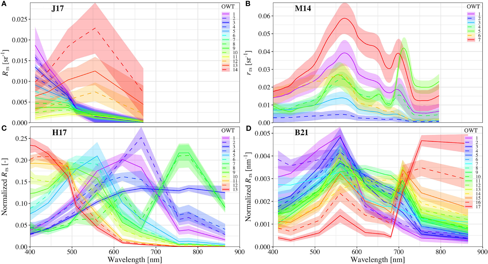
Figure 1 Spectral reflectance of optical water types from four frameworks by (A) Jackson et al. (2017), (B) Moore et al. (2014), (C) Hieronymi et al. (2017), and (D) Bi et al. (2019), and Bi et al. (2021). The line denotes the original spectral centroid of each water type and the shaded ribbon denotes the standard deviation from respective training datasets.
In order to evaluate results of the five AC methods with regard to OWT, four OWT classification methods were selected with different emphases, e.g., focusing on marine or inland waters. For the selection of the OWT methods, it was necessary to consider the degree of affiliation to the cluster centers. Therefore, methods based on fuzzy logic clustering and using the Mahalanobis distance and χ²-distribution to calculate the total membership values were chosen (Moore et al., 2001; Moore et al., 2014). Furthermore, only hyperspectral or at least OLCI band-based OWT methods were selected, but no methods using band ratios or concentration thresholds. For the selection, it was also important to represent a wide variety of spectral forms that are considered important in the different methods. Therefore, in general, other classification approaches could be considered that might provide more robust results for the AC methods under consideration or that are not too focused on either marine or inland waters. The used OWT classification methods are:
1. J17 (Jackson et al., 2017) is an OWT method that was developed in the frame of ESA’s Ocean Colour Climate Change Initiative (OC-CCI). Millions of pixels from merged satellite data were selected for clustering. 11 spectral types for marine waters were identified, and three additional “highly-turbid” coastal spectra from Moore et al. (2014) were also adopted. The original publication referred to the OC-CCI dataset v2 with SeaWIFS bands; in 2020, new optical water class set were defined for the dataset v5 for MERIS-referenced data with POLYMER (v4.12) as the atmospheric correction (Sathyendranath et al., 2021). Thus, the adapted OWT method uses 14 classes and six OLCI bands between 412 and 665 nm.
2. M14 (Moore et al., 2014) uses hyperspectral Rrs between 400 and 800 nm that are primarily representative for coastal regions and lakes, where the centroids were trained based on in situ measurements. The approach distinguishes seven classes, but actually no blue (oceanic) waters. Their original OWT analysis actually refers to the underwater remote-sensing ratio, rrs, which can be transferred above-water to Rrs.
3. H17 (Hieronymi et al., 2017) is a more holistic approach to OWT classification as it aims to cover “most natural waters”, from the open ocean to extremely absorbing or scattering waters. The basis of H17 are radiative transfer simulations with Hydrolight (Mobley, 1994), which is a common approach with the AC methods C2RCC and A4O. The latter was even optimized in terms of OWT classifiability with H17. The OWT scheme uses 11 OLCI bands from 400 to 865 nm and distinguishes 13 classes. In order to avoid conflict with possible negative reflectances, the spectra are transformed by log10(Rrs + 1) and brightness-normalized, so that the classification is based on the shape of the spectrum alone.
4. B21 is an extended OWT framework based on the works of Bi et al. (2019), and Bi et al. (2021), developed specifically for inland waters. The hyperspectral training data, which were resampled to 15 OLCI bands from 400 to 865 nm, were mostly measured at large lakes, reservoirs, and rivers across China. The approach differentiates 17 classes including eutrophic and hypertrophic cases with high biological productivity and even surface scum. The spectra are normalized by dividing them by their integrals because, according to their reasoning, the composition of inland waters varies greatly, which changes the shape of the reflectance spectrum rather than the magnitude.
The selected OWT frameworks have different approaches to classifying the spectra. In H17 and B21 the spectra are normalized (albeit in different ways) to highlight differences in spectral shapes between types, while in J17 and M14 differences in the magnitude of the spectra are taken into account. Therefore, it is expected that the interpretation of atmospherically corrected data will depend in part on the region observed by the satellite, as the different waters for which these methods were initially developed are very different. For example, B21 will not be able to represent oceanic water due to the lack of “blue types”, while J17 will have difficulty distinguishing eutrophic inland waters, which are not foreseen in the marine model of POLYMER, on which J17 is based. In addition to the selected OWT frameworks, we also use the (OLCI) wavelength of the Rrs maximum as a direct and intuitive indication for water types; a similar approach using the spectrally-weighted Apparent Visible Wavelength has been shown to be effective for different optical conditions (Vandermeulen et al., 2020). In general, the maximum reflectance in clear seawater is at shorter wavelengths (more blue or green), whereas in turbid water the maximum is shifted towards longer wavelengths (more green, brown, and red).
In optical fuzzy logic classification, the class membership is calculated by the cumulative χ² distribution with n degrees of freedom (band number) and the Mahalanobis distance between the spectrum and the OWT centroid, normalized by the OWT standard deviation (see calculation details in Moore et al., 2001). To assess the classifiability of an AC-derived spectrum, we calculate the total membership for the OWT classification scheme, ut. An ideal classification result should give ut close to (or even slightly higher than) one. At lower ut, the classification is performing poorly with a threshold on totally non-classifiable defined as ut ≤ 10-8. Such cases can occur either because of insufficient type representation in the framework or because of errors of the spectral shape or intensity itself, i.e., underperformance of atmospheric correction, uncorrected influences from adjacency effects or bottom reflections, etc. (Moore et al., 2014). Jackson et al. (2017) also mentioned that ut should not be much larger than one in the ideal classification result either, which indicates overlap and redundancy between types. However, in this study, we allow ut to be greater than one, because using frameworks across different water areas will inevitably induce overlap between types. We define five levels of classifiability as shown in Table 3. A spectrum is not classifiable if no OWT can be assigned, whereas OWT memberships are distributed between the classes at the other four levels. Evaluation criteria have been discussed in various publications, e.g., Mélin et al. (2011); Vantrepotte et al. (2012), or Hieronymi et al. (2017); the chosen levels are arbitrary, but work reasonably well for the evaluation of the classification. After all, the percentages of classifiable values in the different water types as well as in the entire data set are calculated. The higher the percentage of high or medium values, the better the classifiability of Rrs.
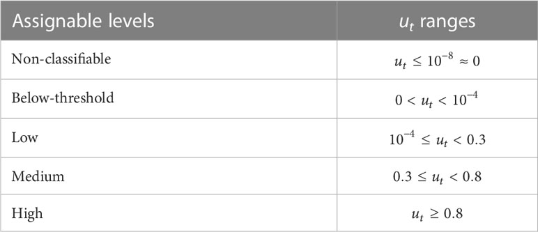
Table 3 Classification levels related to the total membership from all classes.
The various atmospheric correction methods provide individual masks at different levels indicating performance limits and uncertainties (Table 1). Flagging is usually a trade-off between limited validity with suspect results at some spectral bands and still useful results in another spectral range. Many ocean color algorithms utilize only one or a few bands for which the AC results can be adequate. Other in-water algorithms use many bands across the spectrum, e.g., principle component analysis or some neural networks. For OWT applications, the whole spectrum is important. Overcorrection of an AC manifests often in negative Rrs, usually either in blue (especially IPF) or NIR bands; in any case, this is not a physically plausible result and may be an invalid input to the in-water algorithm. Looking at the whole spectrum, IPF and POLYMER produce very large areas with negative reflectances, both about half of the free water area (albeit the values are often very close to zero). The IPF expression for valid pixels requires positive reflectances at least in the central VIS range (412-665 nm), which cannot be satisfied over large parts and is the main reason for >50% invalid masking (Table 4). POLYMER does not have this restrictive flagging, so everything remains valid. Depending on the processing settings, ACOLITE-DSF does not output negative reflectances, but its flagging results as NaN in the output files, which is the main contributor to the 20% invalid flagging (these cases also occur in C2SX waters, for which ACOLITE-DSF was designed, e.g., visible in Figures 2-A5, C5). C2RCC and A4O apply neural networks to approximate log-transformed Rrs directly from RTOA without subtracting individual contributions from Rayleigh scattering or glint. Resulting negative reflectances are ruled out, because of the log-transformation and the value range of the NN training. This is an important advantage with regard to continuous usability of the results with different types of water and allows Rrs estimation even for very small values close to zero with less noise. The slightly more sensitive cloud detection in C2RCC processing with IdePix results in an additional 1% masking of the water areas.
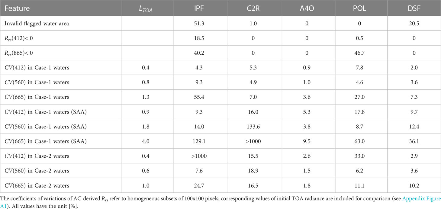
Table 4 Evaluation of selected spatial features for 31.5 million free water pixels in ten test scenes for the five atmospheric correction models.
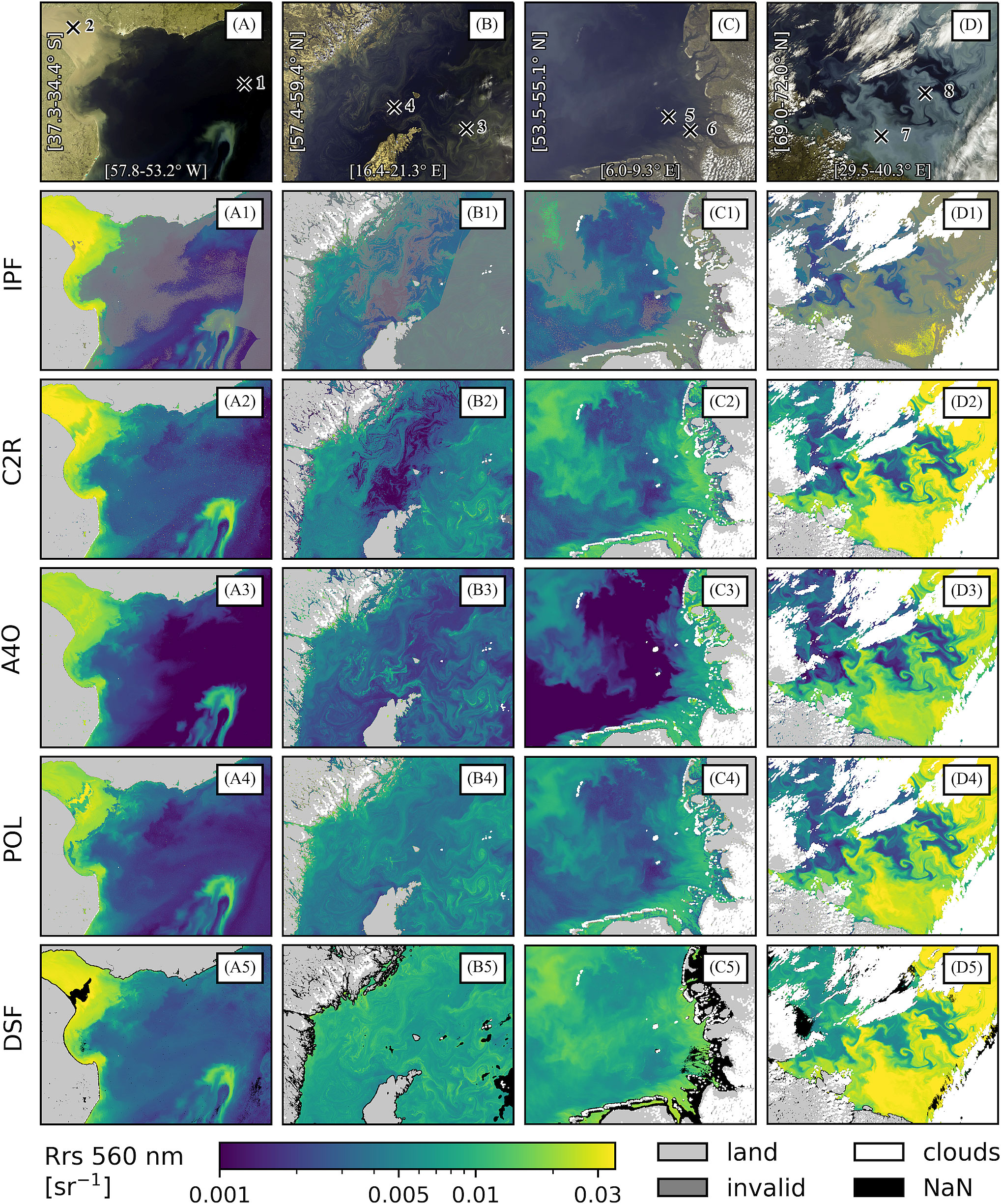
Figure 2 Subsets from OLCI images (see Appendix Figure A1). The top row shows RGB images of L1 radiance at top-of-atmosphere (A–D); points for spectral comparisons are marked there (see Figure 3). The five rows below show the results for Rrs(560) of the compared AC methods: IPF (A1-D1), C2RCC (A2-D2), A4O (A3-D3), POLYMER (A4-D4), and ACOLITE-DSF (A5-D5). Areas of AC-specific invalid pixel expressions are highlighted transparently or with NaN.
Figure 2 shows extracts of satellite images (#3, #7, #2, and #1; Table 2; Appendix Figure A1) of the AC results for Rrs(560) with respective invalid flagging. Spatial noise usually transfers to the ocean color products and is thus an indicator for AC performance. In this context, the South Atlantic Anomaly (SAA) area (Figure 2A) is special; clear spectral outliers of individual bands occur here in isolated pixels and the peaks are usually noticeably higher at longer wavelengths. Some AC methods succeed in smoothing the pixel spectrum, thereby reducing spatial discontinuities. C2RCC produces the most visible noise in this area (Figure 2-A2), which is probably due to the use of neural networks that are very sensitive to small spectral changes. A4O also uses NNs, but has significantly lower spatial noise due to various processing steps, including a dedicated spectral smoothing for suspect outliers and averaging of the results of different NNs (Figure 2-A3). Moreover, an option is recommended for A4O that applies a Gaussian filter over 3x3 macro-pixels, which smooths results for water areas, attenuates cloud artefacts, and tears down camera boundaries. ACOLITE-DSF, as applied here, interpolates atmospheric parameters over a large spatial region, which effectively reduces the AC-induced noise level.
Looking at the spatial homogeneity criterion (CV) at different wavelengths for homogeneous areas of 100x100 pixels (Appendix Figure A1), we see a low and comparable noise levels of the AC-input radiance at TOA for Case-1 and -2 waters; in the SAA area, CV values are about twice as high (Table 4). In Case-1 water in the SAA (scene #3, Appendix Figure A1), we see the biggest differences of CV(Rrs) between A4O and C2RCC, with A4O having the least noise of all the methods. In another (presumably clearer) Case-1 water sea area in the Mediterranean Sea (east of the island Sardinia, scene #5, Appendix Figure A1), the noise of C2RCC is significantly lower and comparable to the other methods, IPF and POLYMER have the highest noise in the red band at 665 nm above the valid-match-up threshold of 15%. In this very clear blue water, Rrs(665) becomes very small and approaches zero. In fact, the variability of Rrs(665) in case of IPF and POLYMER is pure random noise, in A4O water mass structures are still clearly visible and determine CV(665), and in C2RCC one can see weak noisy structures as well. ACOLITE-DSF, which is not designed for such clear water, provides an Rrs(665) image with much higher values compared to the other ACs (factor 10 higher). Because ACOLITE-DSF does not perform pixel-by-pixel atmospheric correction, it shows clear atmospheric structures such as cirrus clouds, which are completely decoupled from the water; in fact, the signal is not only “water-leaving” therefore Rrs(665) is invalid by definition (but not adequately flagged). In another uniform area in Case-2 waters (in the southern Baltic Sea, scene #8, Appendix Figure A1), the noise for IPF and POLYMER in blue bands is very high. In the red band, POLYMER has higher Rrs and therefore less noise here than in comparison with Case-1 waters. Overall, the results from A4O are spatially the most homogeneous over the entire spectrum whereby the noise level is only moderately increased compared to the TOA input signal.
In the presence of undetected, partially sub-visible clouds such as contrails, C2RCC and A4O tend to overestimate the atmospheric contribution, i.e., Rrs is usually lower than ambient. This is less visible for IPF and POLYMER. ACOLITE-DSF does not correct for small-scale clouds by construction. Consequently, cloud artefacts are reflected as amplification of Rrs, increasingly at longer wavelengths (e.g., slightly visible in Figure 2-C5). For small-scale broken clouds, all AC methods have large uncertainties. Spatial inconsistencies related to high optical thicknesses, different aerosol conditions, and cloud shadows are further uncertainty factors (IOCCG, 2019).
A visual comparison of all satellite images shows that POLYMER best dissolves the individual camera borders. A4O and IPF reduce the borders significantly; ACOLITE-DSF and C2RCC often have strong gradients here. POLYMER and IPF deliver particularly good homogeneity across the image width (if Rrs is relatively high). Moreover, POLYMER is the only one that produces relatively homogeneous and consistent results even in areas with high sun glint influence, which means that significantly larger areas from a satellite image can be exploited, e.g., shown by Müller et al., 2015a; Müller et al., 2015b (retrieved spectra from sun glint areas were not further evaluated in this study). A4O and C2RCC also produce results in sun glint, but both with noticeable angular dependencies and uncertainties (corresponding warning flags are partly raised).
However, POLYMER has a specific flaw with occasional discontinuities due to algorithmic instability under some circumstances. Conditions typically affected are dark waters, thick aerosol plumes, low sun elevation, land proximity or strong ocean color gradients. These situations tend to reduce the ratio of “water” signal over “atmospheric” signal. The minimization scheme used in POLYMER reveals those instabilities as vertical stripy artifacts, e.g., visible in Figure 2-A4 or in scene #7. Often these cases are characterized by high reflectance values in the blue. Looking at the entire cloud- and glint-free water surface of all scenes, there is an affected area of approx. 1%, which is, however, not flagged. Coasts, lakes, and rivers are particularly affected by the spatial discontinuities, as they often occur close to land.
In the top row of Figure 2, some points are marked whose Rrs spectra are shown in Figure 3. In the figure, the initial TOA reflectances are also shown dashed with reference to uniform right axes. AC results that are flagged invalid were displayed in dotted lines. The figure illustrates that the solutions of the different AC methods to the same input can be very different. Mostly A4O marks the lower and ACOLITE-DSF the upper result margin. The result of IPF is over large areas of the VIS in the mid-range of the delivered solutions, but often (unnecessarily) flagged. There are indeed some areas where the spectral shape is very similar, only the magnitude is different (points 2, 3, 7, and 8); in this case, the assignment to an OWT class is usually the same. Remarkably, these cases are considered difficult for atmospheric correction, such as in the Rio de la Plata estuary with its high sediment load or with relatively high cyanobacteria concentrations in the Baltic Sea. Nevertheless, both cases exhibit areas that show extreme spatial and spectral discontinuities and incorrect estimations. A good example of this is point 4, where due to very high concentrations of cyanobacteria and possibly floating scum, a significant increase in TOA reflectance occurs in the NIR. Only IPF is flagged invalid here. ACOLITE-DSF has NaN areas near the point, where the invalid-threshold at 1020 nm is reached (Figure 2B). Only A4O and ACOLITE-DSF follow the TOA signal in a plausible way and provide Rrs like those that would be expected in such situations (e.g., Reinart and Kutser, 2006; Qi et al., 2014; Hunter et al., 2016; Bi et al., 2023; Cazzaniga et al., 2023); the other ACs are completely wrong spectrally. C2RCC yields a Rrs spectrum that resembles NAP-rich water and, ironically, is well classifiable in some OWT methods such as H17, whereas, the A4O result is assigned in the correct class but with partly low total memberships. C2RCC provides a discontinuous Rrs(560) image (Figure 2-B2) in the situation with significantly lower values than TOA requires. But on a side note, C2RCC estimates the phytoplankton absorption from the spectrum, from which the L2 product CHL_NN is derived, which in this case yields high concentration values, roughly reflecting the TOA image.
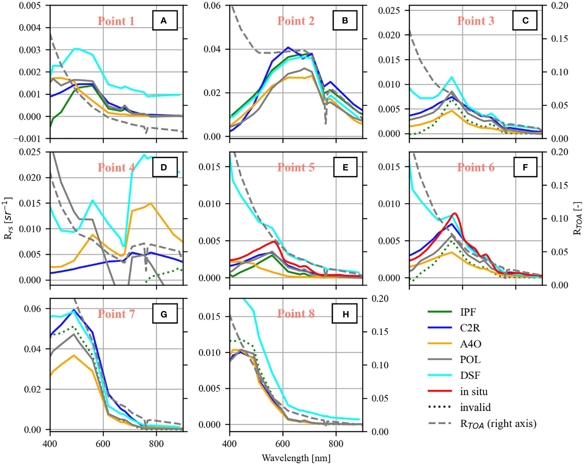
Figure 3 (A–H) Comparison of spectral remote-sensing reflectance derived from the different AC methods for eight points marked in Figure 2. The right axis and the corresponding grey dashed lines show the initial TOA reflectance. (E, F) include corresponding normalized in-situ measurements.
Figures 2D, 3G, H show another example of a phytoplankton bloom, namely coccolithophores, which particularly strongly scatter in relation to the absorption; a sharp gradient is visible from the bright turquoise bloom to the dark blue ocean. The Rrs spectra of the five ACs are similar in both cases and show the high dynamic range of possible values, which is thoroughly comparable with AERONET-OC data during coccolithophore blooms (Cazzaniga et al., 2021).
For many NAP-rich waters, such as rivers and estuaries, one can see similar spectral patterns as in Figure 3B. Often POLYMER and A4O are close together but slightly lower than the other ACs. However, pixels in inland waters that have some distance to land are widely invalid-flagged by the AC methods, only A4O claims to be mostly valid. The 300 m pixel size further limits the usability of OLCI for inland waters and especially rivers. Nevertheless, many lakes are eutrophic or hyper-eutrophic and have comparatively high algae concentrations, often with reflectance features like shown in Figure 3D; here only A4O provides largely plausible spectral shapes (e.g., scene #4, Lake Taihu).
There are in situ data for points 5 and 6 showing the transition from coast to open North Sea; in fact, there would be further match-ups in more turbid water closer to the coast, but ACOLITE-DSF does not provide results there (Figure 2C). It is worth noting that this is the area for which C2RCC was originally developed. It is therefore not surprising that C2RCC performs well here. At point 6, all ACs show a comparable spectral shape, although significantly lower in some cases, especially A4O (Figure 3F). ACOLITE-DSF fits the in situ spectrum very well between 510 nm and the NIR, but at shorter wavelengths there is a strong mismatch, possibly due to the slightly hazy and spatially variable atmosphere. Point 5 is further out in the open sea, where the terrestrial CDOM is largely diluted. At this point, C2RCC, POLYMER, and IPF provide spectra that agree quite well with the measurement (Figure 3E). ACOLITE-DSF fits well between 560 and 620, but otherwise retrieves an overestimated spectrum. A4O interprets the signal incorrectly as a blue ocean spectrum, showing that A4O can have difficulties in the transition zone. It is similar for point 1, but here with even greater variability in the results of the different ACs (Figure 3A). Figure 3 illustrates that in general there are not always consistent results from different atmospheric corrections, which would also be reflected in strongly deviating ocean color products.
Figure 4 shows the comparison of Rrs at selected bands (412, 490, 560, 665, and 865 nm) from match-ups between OLCI A+B data and in situ measurements at nine AERONET-OC stations (colors stand for the individual stations). The results of the five AC methods are shown per row. The contours illustrate the density of the measurements and indicate the 10-, 50-, and 90-percentile lines. Scatterplots do not show the interconnections between the bands, this becomes more visible when looking at the full spectra and evaluating the spectral angle mapper. Thus, Figure 5 shows a subset of data from Figure 4 (from the Black Sea, Baltic Sea, and a lake) from a spectral perspective. In addition, corresponding results of the PANTHYR system from turbid coastal waters are shown in the right column. Some AERONET-OC stations measure at fewer OLCI bands, resulting in different maximum numbers of match-ups per band; PANTHYR measures hyper-spectrally (but band averaged data are used for the comparison).
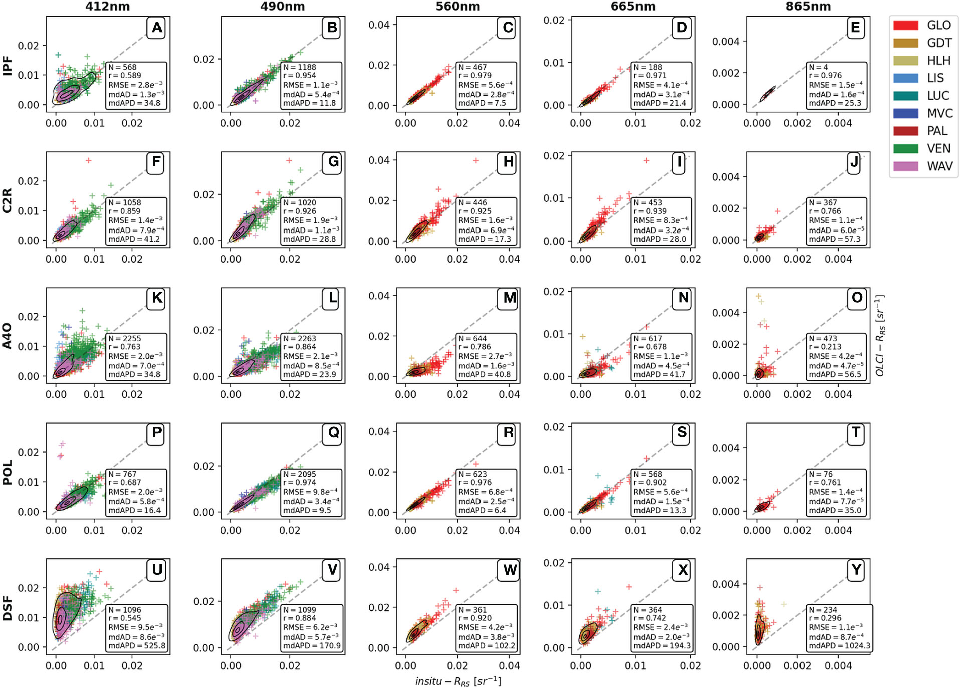
Figure 4 Comparison of satellite-derived Rrs with AERONET-OC in situ data for OLCI bands at 412, 490, 560, 665 and 865 nm for IPF (A–E), C2RCC (F–J), A4O (K–O), POLYMER (P–T), and ACOLITE-DSF (U-Y). The colors represent different stations. The contours indicate the density distribution.
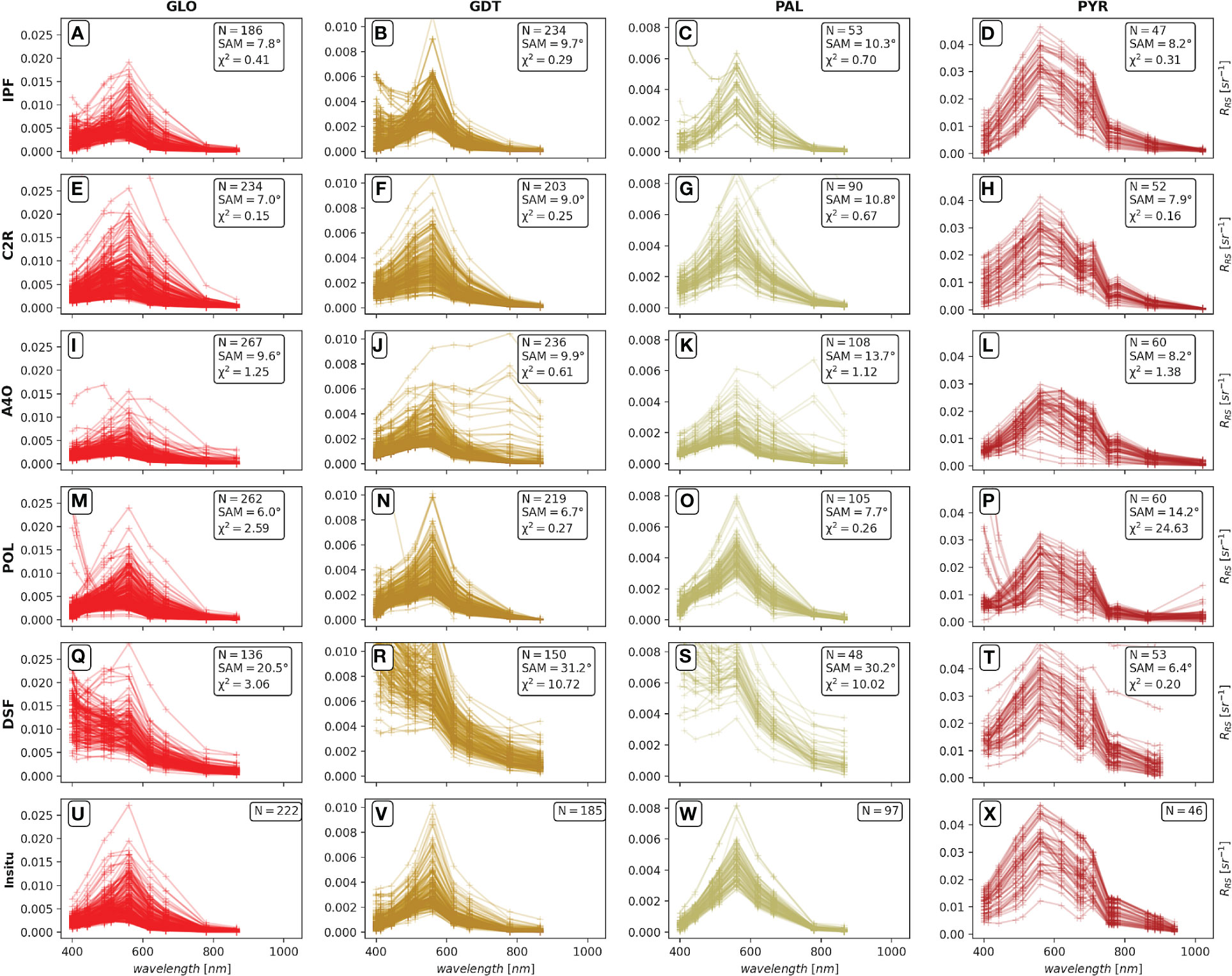
Figure 5 Satellite-derived Rrs spectra of IPF (A-D), C2RCC (E-H), A4O (I-L), POLYMER (M-P), and ACOLITE-DSF (Q-T) compared with in situ data (U-X) from selected AERONET-OC stations (Gloria, Gustav Dalen Tower, Palgrunden) and PANTHYR (right). The statistical parameters refer to complete spectra at ten OLCI bands.
The already mentioned findings on AC flagging and especially the spatial homogeneity criterion (Table 4) are reflected in the number of valid match-ups. Due to the very low noise level, A4O yields significantly more accepted match-ups with AERONET-OC than all other methods, in blue bands at least twice as many points (at 412 nm N = 2255) and in the NIR, for example, 473 vs. 4 points from IPF. Additional warning flags can often identify clear outliers, which are incorporated into the determination of statistical performance, as can be well seen in Figure 5. The obvious outliers in A4O (all associated with clouds) are few and far less than the match-ups sorted out else (Figures 4K–O, 5I–L). Due to the very large differences in individual match-ups, the following analysis does not include a Common Best Quality approach (Müller et al., 2015a).
With respect to the IPF, the retrieved Rrs agree quite well with the AERONET-OC data, with the exception of a number of data points with overestimation in blue bands (considering that many negative values are not taken into account due to masking, see Table 4). The slopes of the regression lines are very close to one. The correlation coefficients for the bands 490 nm to 865 nm range from 0.954 to 0.979; in the blue spectral region, it is significantly lower at 0.589. For PANTHYR data, the correlations are also high, namely >0.85 for all bands except at 412 nm, where r = 0.493. In fact, IPF’s correlation coefficients for central VIS bands are among the highest and RMSE/deviations are among the lowest for both datasets. However, there are insufficient matches in the NIR to meaningfully evaluate the performance. Compared to the other ACs, the number of valid data is lowest for the blue, red, and NIR bands. Mainly the invalid flagging due to negative reflectances as well as the noise-related uncertainties are responsible for the big loss of match-ups. The spectral comparison reveals the partial difficulties of IPF in short wavelengths, but on the whole the good agreement with the measured reflectances, obviously in comparison with the C2S/X data too (Figures 5A–D). An occasional discontinuity of the first three bands is also visible in Figure 3; this could have an influence on OWT applications.
The C2RCC processing in this work includes SVC gains (sometimes not done), which are particularly effective in blue bands. Thereby C2RCC achieves the highest correlation (0.859 for AERONET-OC and 0.618 for PANTHYR) and smallest RMSE (0.0014 and 0.0046) in the blue band at 412 nm (but not smallest deviations mdAD or mdAPD). C2RCC tends to retrieve slightly overestimated Rrs; all biases are positive. With respect to our complex-water-dominated data set, Cazzaniga et al. (2022) conclude similar assessments for C2RCC, but for comparisons with clear waters, they show a general underestimate of reflectance from C2RCC. However, the correlation coefficients are high for the entire spectrum, even at 865 nm, in both cases r > 0.76, but the values are more scattered than, for example, for IPF or POLYMER. The spectral comparison shows good agreement in all orders of magnitude of the measured values; χ² and SAM are generally among the lowest (Figures 5E–H). This implies a potentially good classifiability for Case-2 waters, for which C2RCC was optimized.
For A4O, this is the very first comparison with AERONET-OC or PANTHYR in situ measurements. Despite the very high number of match-ups that were achieved by A4O, which suggests that potentially difficult cases are included in the assessment (but not in the other methods), clear statistical correlations can be demonstrated. All outliers visible in Figures 5J, K (both Baltic Sea) are exclusively related to cloud margins and often recognizable algal blooms in the vicinity. Nonetheless, a medium to strong positive linear correlation is achieved for all bands except the NIR, which is corrupted by some outliers (despite that, the lowest absolute deviation is obtained in the NIR). A4O reaches the second best correlation for blue bands with a value of 0.763; in contrast, in the important green band at 560 nm, A4O has the lowest correlation coefficient in comparison with the other ACs (0.786). There is a clear tendency that values are underestimated in the central VIS. This becomes visible in Figures 5I–L (and Figure 3) too and is echoed in χ². However, apart from few outliers and partly lower values, A4O shows a very similar spectral shape as the measured values. This holds also true for the turbid scattering waters (Figure 5L), but two “false blue” spectra appear as well, similar to the coastal-ocean transition zone in Figure 3E.
POLYMER applies not such rigorous flagging as IPF, so the main factor for relative loss of match-up points comes from spatial homogeneity of low reflectances (CV). The in situ data used here are more representative of Case-2 waters, where POLYMER’s noise in blue bands is relatively high (Table 4), as shown by the relatively low N at 412 nm (Figure 4P), but this is also true for NIR bands (Figure 4T). However, POLYMER and A4O deliver the most match-ups in the central VIS, with more than 2000 at 490 nm, twice as many as at IPF, C2RCC, or ACOLITE-DSF. The statistical characteristics prove the very good performance of POLYMER; but in C2SX waters, the values are only in the average range with the worst evaluations of all ACs in the blue band. Nevertheless, some outliers significantly affect the metrics, well visible in the spectral plots; these are usually associated with the mentioned strip-like spatial inconsistencies (e.g., visible in Figure 2-A4 or scene #7 in the Gulf of Finland). Admittedly, POLYMER has corresponding warning flags that partly identify these cases, but also mark many productive waters. In principle, the spectral shape from POLYMER is well reproduced, although occasionally with recognizable residuals from the polynomial regression in the shorter wavelength range. Usually, these features are not found in in situ measurement data (Figures 5M–P), so this can become problematic for correct OWT identification again.
This is also the first comparison of ACOLITE-DSF for OLCI products with AERONET-OC data. Apart from the blue bands, slightly better correlations can be obtained than with A4O, at 560 nm, r = 0.92. In general, an overestimation of reflectance is recognizable, with the highest values for RMSE, mdAD, mdAPD, SAM, and χ² everywhere. The overestimation is caused by use of the minimum aerosol optical thickness retrieval in an image sub-tile, leading to an underestimation of atmospheric reflectance and hence overestimation of water reflectance. This clearly becomes a significant uncertainty when the water signal is very low compared to the atmospheric signal, as it is here for the AERONET-OC match-ups. For waters with relatively low reflectance values in the blue (in principle, especially C2A/X), there are clear shape problems that are critical for OWT applications. The agreement with measured values is significantly better for the C2S/X waters for which ACOLITE-DSF was developed. SAM and χ² are among the smallest here, this also applies to the central visible range for RMSE, mdAD, mdAPD; however, the correlation coefficients are among the lowest. ACOLITE-DSF gives results close to the 1:1 line for PANTHYR data for all bands (not shown); all other AC methods underestimate the reflectance, sometimes significantly.
The OWT analysis of cloud- and sun-glint-free water surfaces refers only to the individual flags for invalid AC, spatial homogeneity is not taken into account. As already noted, invalid masking leads to 51% and 20% data loss for IPF and ACOLITE-DSF, respectively (Table 4). If one ignores the masks in IPF, one actually gets very similar OWT class distributions. In principle, the OWT methods can exploit slightly negative reflectances.
Figures 6, 7 show percentage distributions of the levels of OWT classifiability of AC-derived Rrs using four different OWT classification schemes. The numbers above the bars in Figure 6 (except for the last three columns) illustrate the percentage allocation of classes with maximum memberships in the OWT frameworks (see Figure 1 for the spectral shapes). The numbers in the color bars indicate the percentage of the assigned classification level (if >10%), all classifiable contributions sum to 100%. In the example of IPF and J17 in Figure 6A, 21% of cases with maximum membership in class 1 have medium (0.3 ≤ ut< 0.8) total membership and 78% have only low membership (10-4 ≤ ut< 0.3). The total fraction of spectra of class 1 is less than 0.1% of all IPF-J17-classifiable free water pixels (for such small fractions, the value is not written above). Figure 7 shows the corresponding distribution of classification results but sorted by the OLCI waveband with the maximum reflectance provided by the AC method. Each subplot in Figures 6, 7 includes three additional bars: “ALL” summarizes the total distribution over all pixels including non-classifiable and flag-invalid pixels; “BLOOM” considers cases that are flagged with the FLOATING mask of A4O with the characteristic red edge enhancement of RTOA, this is typical for intense cyanobacteria blooms; and “C2SX” is for waters with Rrs(865) ≥ 0.005 (depends on AC). C2SX and BLOOM are typical cases for coastal and inland waters. The distributions in C2SX (yellow numbers) and BLOOM (green numbers) refer to different numbers of total valid pixels per AC, e.g., only 5% of the BLOOM pixels are not flagged and therefore valid in IPF, but 100% are valid in A4O. When interpreting, one should keep in mind that the shape of the reflectance provided may be wrong for the given situation, but the spectrum may be well classified in a different class. Orange colors in Figures 6, 7 represent the level with too low contributions of the classes to be considered “classifiable”; this shows the potential of relaxing the threshold (10-4) and indicates too narrow tolerance for class memberships of the OWT systems.
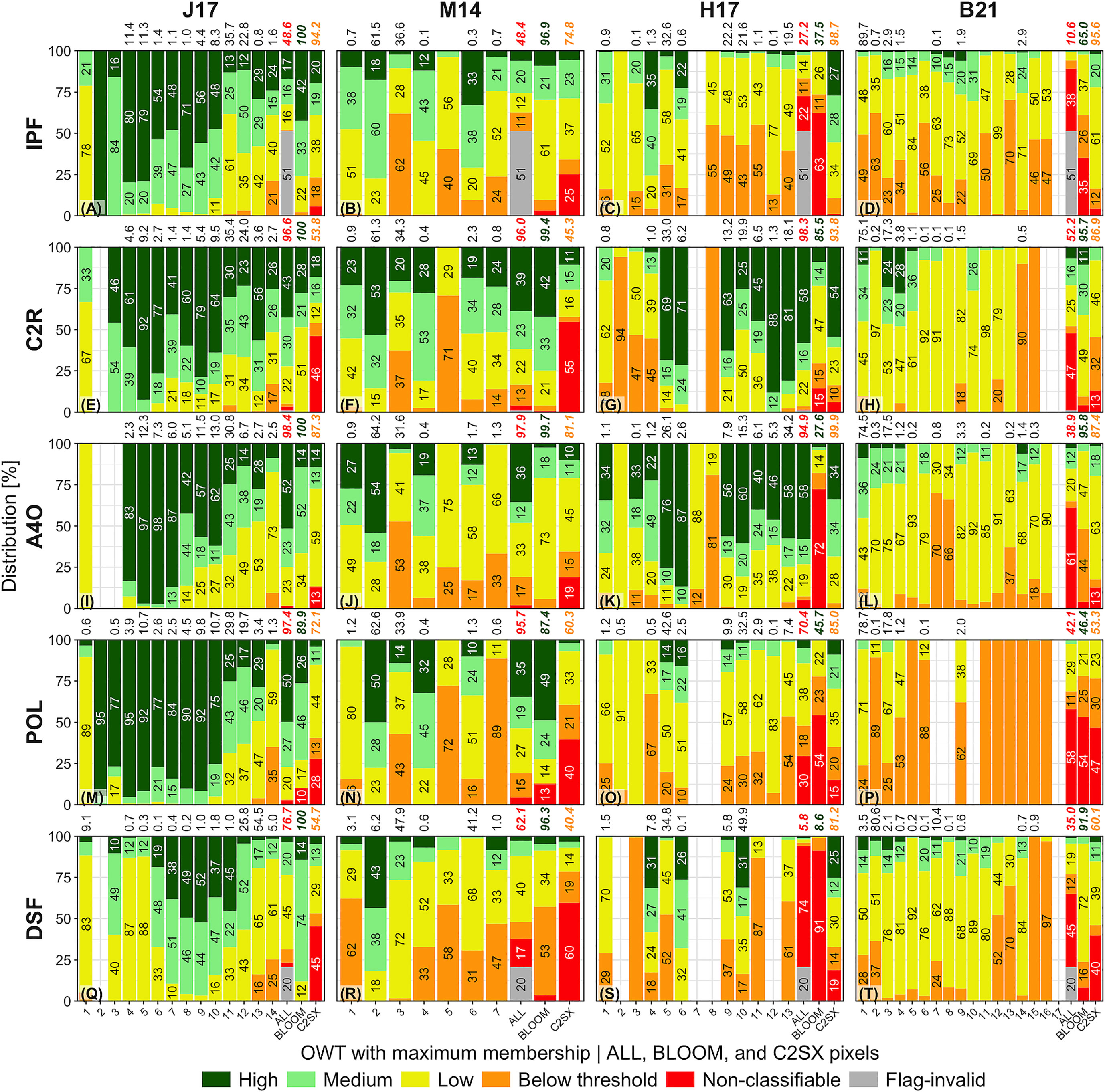
Figure 6 OWT classifiability of AC results of IPF (A-D), C2RCC (E-H), A4O (I-L), POLYMER (M-P), and ACOLITE-DSF (Q-T) for free-water pixels from ten OLCI scenes using four OWT methods with different numbers of classes. X-axis: OWT class allocation with maximum memberships, the last three columns each show total distribution for all pixels (31.5 million = 100%), only pixels with floating algae (BLOOM, <0.6% of all), and only extremely scattering waters (C2SX, 4%). The percentage of classifiable pixels is noted at the top (not shown if the share is smaller than 0.1%) and related to the total percentage share, which is indicated as a red number. Y-axis: distribution of total class membership for classifiable pixels (total memberships >0; see Table 3). Empty spaces show that the class is not present.
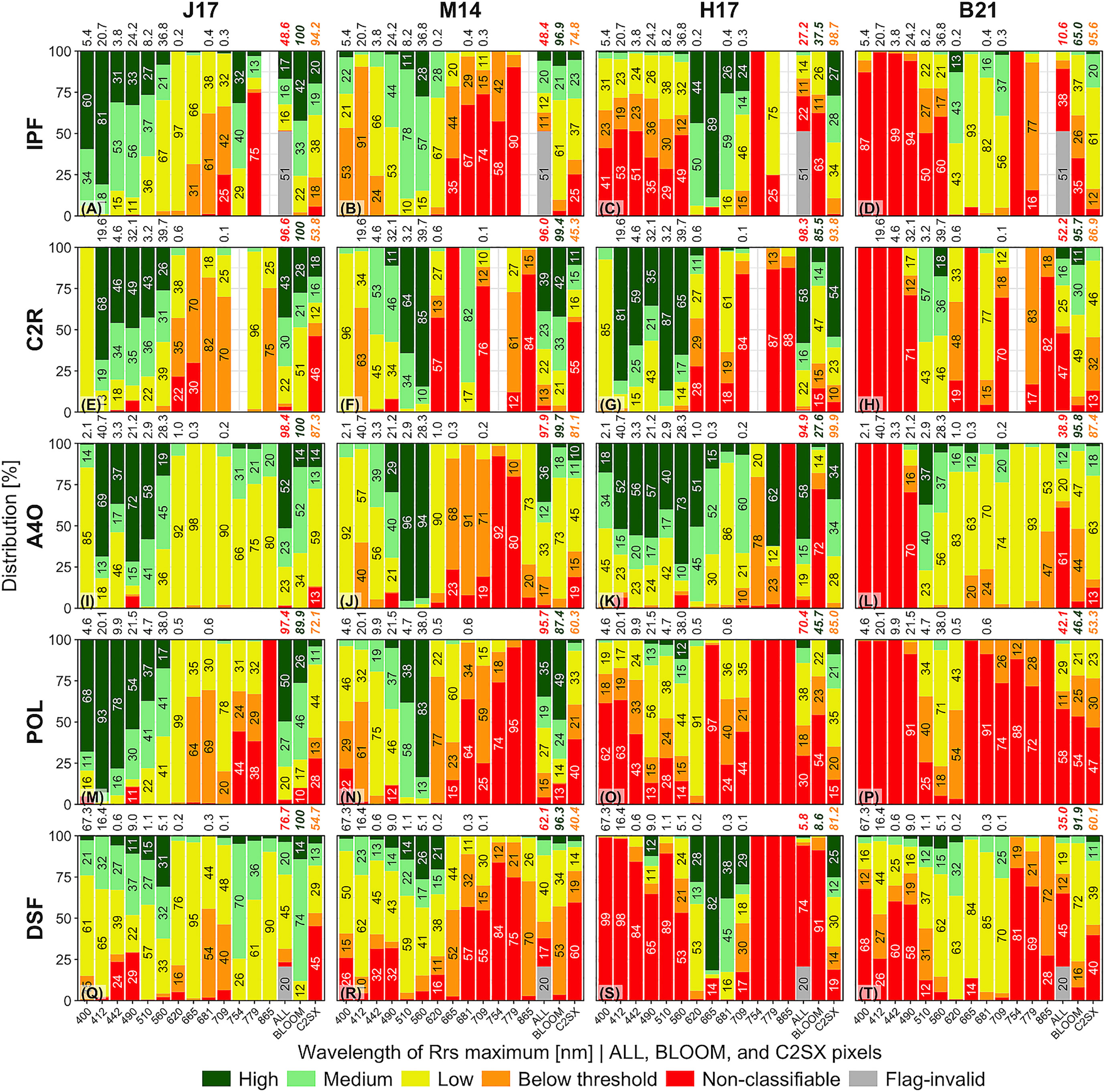
Figure 7 Same OWT classifiability of AC results as in Figure 6, but at X-axis with the OLCI wavelength of the Rrs maximum and corresponding percentage distribution noted at the top (this distribution is independent of the OWT method and therefore the same for all).
First, let us analyze the total distributions sorted by wavebands with satellite-derived Rrs maximum (Figure 7). There are some differences visible between the five AC methods, although the absolute numbers are not equally representative since some features occur rarely in the test scenes. However, the distributions of IPF, C2RCC, and POLYMER are quite comparable, with roughly 20% at 412 nm, 20-30% at 490 nm, and 40% at 560 nm. A4O has about 40, 20, and 30% of these bands, resulting in roughly twice as many “blue” spectra. ACOLITE-DSF has in more than 67% of cases an absolute Rrs maximum at the first band (400 nm), further 16% at 412 nm, 9% at 490 nm, and only 5% at 560 nm. Typical examples of this spectral behavior can be seen in Figures 3, 5Q–T. This blue maximum is characteristic of atmospheric path reflectance and indicates again the under-correction by ACOLITE-DSF for low reflectance targets.
J17 is the OWT framework that utilizes the least bands as input, which is favorable for obtaining higher membership values, and focuses on ocean and coastal waters. Moreover, J17 was developed based on satellite data that were atmospherically corrected with POLYMER. It is therefore not surprising that POLYMER has the greatest distribution of water types and overall good classifiability per class; the classifiability only degrades for the turbid water classes (Figure 6M). POLYMER, C2RCC, and A4O each achieve >70% high or medium total memberships, indicating good classifiability. Without invalid masking, IPF would come to a similar level; with masking, it achieves only 33%. ACOLITE-DSF only reaches about 20%. ACOLITE-DSF mainly produces four types of spectra, turbid (85% in OWTs 12-14) or very clear water (9% in OWT 1), but mostly with low memberships. In the used test scenes, the first three classes of J17, representing oligotrophic ocean water, are almost non-represented in the other ACs (still 1% in POLYMER). J17 lacks specific classes for C2SX and eutrophic waters (BLOOM); if the AC produces such spectra, they are assigned elsewhere or are not classifiable – the same holds true for the other OWT schemes. Of the (in IPF only 5%) valid BLOOM pixels, most are well-classifiable; however, in C2RCC, the spectra often look like scattering waters, which are less well classifiable (only 49% good). C2SX waters occur much more frequently in the scenes, whereby particularly high spectra (such as in Figure 5X) are not classifiable. This is one of the reasons why A4O, with its potential underestimation of reflectance, achieves better classification results. Given the diversity of spectral maxima, A4O consistently provides useful memberships, even in rare cases with Rrs maximum at bands >560 nm (Figure 7I); but also IPF and ACOLITE-DSF provide many well classifiable spectra for these cases.
M14 focuses on coastal and inland waters with the fewest classes. The class distributions and classifiability of valid results from IPF, C2RCC, A4O, and POLYMER are comparable. More than 95% fall into OWT 2 or 3 with 48 (A4O) to 62% (C2RCC) well-classifiable cases. ACOLITE-DSF produces a different class distribution with 48% in OWT 3 and 41% in 6, where overall the reflectances are less classifiable. Waters with high NAP concentration are often non-classifiable, only A4O achieves up to 81% classifiable results. In the case of red edge enhancement (BLOOM), A4O yields reasonably correct spectra, but achieves only lower memberships with M14 than the sometimes certainly incorrect results of C2RCC and POLYMER (as Figure 3D).
H17, just like A4O and C2RCC, was developed on the basis of Hydrolight radiative transfer simulations considering comparable inherent optical properties for the marine model, furthermore all three methods operate in a log-transformed form, therefore the two ACs have advantages here. Particular emphasis is placed on the spectral shape and the allowed variances are quite narrow in the H17 scheme, so that even relatively small deviations can lead to poor classification results. In fact, reflectances from IPF and ACOLITE-DSF are practically unclassifiable with H17, but almost all pixels with C2RCC and A4O with 74% medium or high memberships are. Only half of the POLYMER reflectances can be classified as having weights above the threshold, but total membership remains mostly low. Insufficient memberships are usually found in highly scattering or productive waters, or when POLYMER provides negative reflectances in Case-1 waters. A4O matches all defined classes, but has low memberships for productive waters OWTs 7-8, that are masked with BLOOM. The reason for low memberships is likely the particularly high variance of natural Rrs at NIR bands, which is not well captured by the H17 χ²-distribution. However, it is important that the class is identified correctly, which enables post-classification adaptation for optimal water algorithm selection. All other ACs do not deliver such spectral shapes; (wrong) C2RCC can be relatively well classified. The majority of spectra provided by IPF, POLYMER, or ACOLITE-DSF with the maximum in the short wavelengths (<560 nm) are not classifiable with H17, bright pixel spectra of IPF and ACOLITE-DSF, however, are often well classifiable. This shows that low reflectance values play a major role in the log-transformed classification and that the associated noise-level of some bands leads to shape variations not expected by H17.
Method B21 distinguishes most classes but has a focus on inland and coastal waters with little regard for the ocean. In addition, the shape is also given more consideration here, and the allowed variations are fairly limited. None of the AC methods succeeds in providing comprehensive spectra that can be classified with the method of B21. For C2RCC, nevertheless, half of the pixels are classifiable with ut above the threshold (>10-4). For all ACs, at least 85% of the classifiable cases are distributed among the first three OWTs; the other 14 classes are sparsely used. C2RCC, A4O, and ACOLITE-DSF yield >90% usable spectra for BLOOM-labelled pixels. Again, C2RCC provides a higher percentage of well-classifiable results, but these are not in the intended classes (OWTs 14-17). A4O provides such spectra, the majority of which have useful memberships. Figure 7T shows slight advantages for the classifiability of ACOLITE-DSF spectra with the maximum in shorter wavelengths.
Inter-comparison results are often a snapshot in time, as both AC and water algorithms undergo continuous evolution. This paper refers to the most recent AC versions (as of October 2022) and is authored by some of their main developers. It is clear that the methods are at different maturity levels and that some have been optimized using observational data, which is also reflected in the effort for uncertainty products and flagging. A4O by Hieronymi et al. is a further development of C2RCC, but is not yet publicly available and there is no official reference for it as well. IPF is used in operational service, but one must also appreciate the continuous developments, where with the OLCI Collection-3 (since 2021) improvements have been achieved, e.g., for coastal waters (Zibordi et al., 2022). One cannot say that this is a Case-1 ocean color specific algorithm anymore, because the comparisons with Case-2 dominated match-up data document good agreement over most of the spectrum (with specific problems described here). Our comparisons with AERONET-OC and other data show better agreements for IPF than previously reported (especially also with regard to the previous IPF version Collection 2), e.g., Liu et al., 2021; Tilstone et al., 2021; Vanhellemont and Ruddick, 2021; Li et al., 2022; or Windle et al., 2022. One influencing factor is certainly the consideration of recommended flags and the use of the same IPF-SVC gains for all AC methods (except for POLYMER). Ideally, AC-specific SVC gains should be used, but these are not yet available for C2RCC, A4O, and ACOLITE-DSF; specially fitted SVC would have the potential to significantly improve their results. In the mentioned studies, likewise other versions of C2RCC, POLYMER, and ACOLITE-DSF are used; nevertheless, some similar observations can be confirmed, like the principal suitability of C2RCC and POLYMER for Case-2 waters especially for the central visible range. A4O and ACOLITE-DSF have partly less favorable ratings compared to AERONET-OC data, but both procedures are currently undergoing a greater dynamic in their development (they have undergone several updates in 2022). For all ACs, suitable methods must be found in the future to better identify obvious outliers in order to achieve better spatial and statistical evaluations. This also includes even better cloud identification. Considering the strict invalid flagging of IPF, however, one potentially loses considerable amounts of observational data, which should be reconsidered.
Spatial homogeneity, which has a strong impact on the number of match-ups, should be given more attention in future. For this purpose, measures to homogenize atmospheric properties at macro-pixel level (A4O & ACOLITE-DSF) as well as the log-transformation of the Rrs retrieval for very small values (A4O & C2RCC) have proven to be efficient. In combination with spectral smoothing (as in A4O), this is also advantageous for large areas affected by the South Atlantic Anomaly. One may argue that using a non-strict pixel-by-pixel atmospheric correction limits the high spatial resolution (of up to 300 m), however, relevant atmospheric and oceanographic features are usually larger in area and AC-induced noise is a significant source of uncertainty for ocean color products.
High accuracy over all magnitudes of retrieved Rrs is expected over the entire spectral range for various applications. Recent reviews summarize the requirements for ocean color remote sensing and especially atmospheric correction, e.g., in terms of deriving inherent optical properties of water (Werdell et al., 2018), phytoplankton diversity (Bracher et al., 2017), carbon content (Brewin et al., 2023), and essential biodiversity variables (Muller-Karger et al., 2018) – and this goes beyond the OLCI bands, also for future hyperspectral applications.
The selected AC method has often a significant influence on the derived ocean color products, e.g., the estimate of the concentration of carbon in water or the phytoplankton biomass with corresponding primary production. Juhls et al. (2022) for example compared in situ data with OLCI match-up results from IPF, C2RCC, and POLYMER and, moreover, different models for the estimation of CDOM absorption. This was done in order to investigate fluxes of related dissolved organic carbon from a large river across the turbid coastal zone into the clear Arctic Ocean, thus in high latitudes (here, POLYMER is identified as the most suitable). The strongest optical effect of CDOM is visible in the blue bands, where, according to our study, C2RCC and A4O have slight advantages also in terms of noise and spectral behavior; ACOLITE-DSF has noticeable problems. In this example, the actual performance may be inconsistent along the optical gradient, especially at short wavelengths; OWT-optimized water algorithms could potentially contribute to reducing the uncertainties (if the classification is successful).
Concentrations of phytoplankton in the order of Chl > 1 mg m-3 are usually necessary to hyper-spectrally distinguish special pigment absorption features and thereby phytoplankton diversity; moreover, the central visible range (450 to 650 nm) is particularly important for that (e.g., Xi et al., 2015; Xi et al., 2017; Bi et al., 2023). The intensity and spectral shape of the reflectance in the case of “moderate” algal blooms are generally well reproduced by all AC methods investigated (e.g., Figure 3C). Results from the current version of A4O, however, mostly show an underestimation (which may also have to do with influences of the angle normalization that still need to be clarified). At higher Chl (>10 mg m-3), the red edge absorption feature becomes important in the Chl retrieval (e.g., Gons, 1999; Ruddick et al., 2001). High concentrations of cyanobacteria with possible scum at the water surface, which is a frequent phenomenon in inland waters and the Baltic Sea, are a particular challenge for AC. Spectra from IPF, C2RCC, and POLYMER are mostly untrustworthy here and the results are partly not sufficiently accompanied by warnings (Figure 3D). A4O, which has a specific warning flag for this, provides a plausible spectral shape and indicates enhanced Rrs uncertainties in corresponding products (which is also reasoned by the usual small-scale heterogeneity of such blooms). The spectra from A4O can be assigned to the designated water classes in H17 and B21, but often with low memberships. In the shown example (Figure 3D), the shape of ACOLITE-DSF is also plausible except for the first two bands that are likely overestimated and may be impacted by smile correction artefacts (the spectra are usually not well-classifiable in H17 or B21). However, there is a possible advantage of the dark-spectrum-fitting approach in the range 500-700 nm, which can be helpful for phycocyanin feature detection (a marker for cyanobacteria).
The other example with a bloom of coccolithophores (Figure 3G) shows comparable spectral shapes delivered by all ACs, but also clear differences in the brightness of the retrieved reflectance (although all results are of a realistic order of magnitude, e.g., Cazzaniga et al., 2021). Methods to remotely sense particulate inorganic carbon focus on optical detection of coccolithophores, e.g., with a color index made from ratios of green, red, and NIR bands (Mitchell et al., 2017; Brewin et al., 2023); here significant differences would occur depending on the AC used. Regarding the exploitation of red and NIR bands in ocean-water algorithms (also important for the estimation of the fluorescence line height), the spatial homogeneity and negative reflectances are improvable for IPF and POLYMER, and the removal of artefacts from small-scale atmospheric variability for ACOLITE-DSF.
The distinction of optical water types is important for many aspects of marine biology, physical oceanography, underwater visibility, etc., and the definition of specific properties has a long tradition (e.g., Jerlov, 1976). Current research aims to determine reliable water quality characteristics from satellite data for the entire aquatic continuum of land-coast-ocean. However, a balance between effort and benefit must be found here and care must be taken in satellite images to ensure no unwanted discontinuities arise. There may be specific challenges for oceanographic or limnological questions, e.g., with regard to water constituents, sun glint, whitecaps, shallow water, or adjacency effects, but from an optical remote sensing point of view, it does not make much sense to reduce oneself to one application. This common disconnection actually hinders reliable studies on matter transfer from land to the sea, which is important for the carbon cycle, for example.
The lack of classes with characteristic optical features is a problem for all OWT methods that were examined, e.g., classes representative of oligotrophic ocean, very high NAP concentrations, or hyper-eutrophic waters are often missing. On the other hand, there may be spectral classes that are difficult to explain from an IOP perspective. Especially inland water OWT frameworks are often based on clustering of large in situ data collections, which include potential measurement errors such as adjacency effects, bottom reflections or inadequate sky-glint correction. Consequently, classes with questionable mean reflectances can also be defined. Some OWT frameworks are primarily used to evaluate the quality of Rrs spectra (e.g., Wei et al., 2016). An independent control is the Quality Water Index Polynomial (QWIP) method of Dierssen et al. (2022). The QWIP score for hyperspectral data should not exceed 0.2, for multispectral data as for OLCI the nominal threshold can be relaxed to 0.3, values above the threshold should be subject to additional checks. In fact, the QWIP method does not include “green types” with Rrs maximum in the NIR, such as defined by B21. However, few classes of B21, e.g., their OWT 2, receive a QWIP score close to 0.2 (note that some OWT frameworks like Spyrakos et al. (2018) define classes with higher scores that possibly fail the QWIP quality control). The B21 OWT 2 class-mean spectrum has a local minimum at 440 nm (Figure 1D). Our OWT analysis shows that B21-classifiable spectra of IPF, C2RCC, A4O, and POLYMER are in this OWT 2 with less than 1%, whereas 80% of ACOLITE-DSF spectra fall into this class. The comparisons with AERONET-OC indicate an underestimation of the atmospheric signal of ACOLITE-DSF in blue bands; furthermore, there is reason to conclude that adjacency effects, e.g., from bright clouds, play a role (Bulgarelli and Zibordi, 2018). Indeed, QWIP can be used directly for quality control for satellite-derived Rrs, e.g., Turner et al. (2022) compared results from ACOLITE-DSF and POLYMER (in other versions) as well as the standard NASA SeaDAS algorithm for OLCI (L2gen) for an estuary at the US East Coast finding POLYMER to be the preferred approach. Applying the QWIP score to the AC results of our study for valid free water pixels in the scenes and assuming a threshold of ≤0.2 gives 100% reliable Rrs for A4O and C2RCC, 99% for POLYMER, 81% for IPF, and 45% for ACOLITE-DSF. With a less stringent threshold of ≤0.3, ACOLITE-DSF achieves about 88% quality-assured Rrs. With a very strict QWIP score of ≤0.1, A4O still reaches 99.4%. This means that virtually all results from A4O, C2RCC and POLYMER pass the QWIP quality control with slight advantages for A4O. But as mentioned, the retrieved Rrs can actually have the “wrong” shape.
The ability to fill all classes and generally good classifiability of reflectances from POLYMER in the J17 framework or from A4O in H17 shows the great advantages of matching AC and OWT frameworks. As described, however, there is a danger of over-valuing false spectra from the AC or measurements/simulations. Nevertheless, it has also proven ineffective not to allow large variances from the expected spectrum, i.e., potential errors of the AC. Obviously good spectra from IPF or POLYMER, but also from A4O, cannot be classified well with H17. This is especially true for B21, where in principle the results of all ACs do not fulfil the expectations.
A comprehensive evaluation of the OWT systems and of the performance of different atmospheric corrections is difficult because the actual areas of application and validity overlap sometimes only slightly, i.e., inland waters vs. ocean. Large areas of inland waters are invalid flagged or at least have warning flags raised, so it is not surprising that almost all data fall into one or only a few designated ocean classes for M14 or B21. However, some of the AC methods give plausible and usable results for inland waters, which is partly evident in the comparison with AERONET-OC. Leaving aside the fact that there are also erroneous estimates of the Rrs shape, C2RCC and A4O produce classifiable results of at least 95% of the cases in the OWT frameworks J17, M14, and H17, where A4O covers more intended classes. POLYMER also achieves this classifiability rate for J17 and M14, but only 70% for H17. Considering the recommended flags, the suitability of IPF and ACOLITE-DSF in the investigated classifications is insufficient. The work by Liu et al. (2021) also compares IPF, C2RCC, POLYMER, and other OLCI AC methods in context with the optical water type and quality control framework of Wei et al. (2016), which differentiates 22 classes; they conclude that POLYMER has best performance followed by C2RCC and IPF.
Figure 3A illustrates a remaining problem, namely that fundamentally different spectral shapes of the derived Rrs can often occur in the transition from coast to sea, when the freshwater CDOM concentration is diluted. In some cases, there are features in the TOA signal that can be used to flag potential uncertainties, e.g., a red-edge enhancement (Figure 3D). The ambiguities of the optical effects of different components in the water, at the air-sea interface, and in the atmosphere are relatively large for spectrally smooth TOA reflectance with color nuances of blue. Without systematic comparisons with suitable in situ data, we have no means of determining which spectral shape is correct, i.e., which OWT is present. For this purpose, more hyperspectral fiducial reference measurements especially with maximum Rrs at wavelengths ≤510 nm are needed.
Five atmospheric correction methods for Sentinel-3/OLCI ocean color imagery were compared in terms of spatial and spectral results and individual flagging. The models under investigation are the most recent versions of OLCI L2 baseline atmospheric correction (IPF), C2RCC, a new method A4O, POLYMER, and ACOLITE-DSF. The extent to which AC methods provide useful and continuous results for a wide variety of natural waters was investigated. For this purpose, the satellite-derived remote-sensing reflectances were evaluated in four optical water type schemes.
Flagging leads in some cases to major limitations in data exploitation even for clearly visible water areas; IPF recommends very strict criteria, resulting in 50% less coverage in our satellite imagery. Output of Rrs with negative values is a major issue here. However, we have also shown that many cases are inadequately flagged by the AC methods; an example are high concentrations of cyanobacteria at the sea surface. Only A4O has a dedicated warning flag for floating algae, but A4O is valid here and delivers as the only one reasonable Rrs over the entire spectrum. Nevertheless, a revision of the individual flags with respect to spatial and spectral inconsistencies is recommended for all AC methods. Cloud and cloud shadow detection also need to be improved for all methods, as corresponding deficiencies are reflected in the derived water quality products.
Pixel-based approximation of atmospheric properties and reflectance leads to AC-induced spatial noise. High spatial heterogeneity, especially at low reflectance (and overcorrected negative values), leads to considerable losses of possible match-ups with in situ measurement data. The noise level can be effectively reduced by means of log-transformation in the Rrs retrieval process and appropriate smoothing, which is both applied in A4O. Mainly because of its high spatial homogeneity, A4O achieves significantly more match-ups with AERONET-OC data than all other methods, namely at least twice as many points in the blue and NIR bands. The number of match-ups achieved also affects the statistical evaluation of Rrs retrieval performance. Comparison with in situ data, which are more representative of coastal and inland waters, shows that the spectral shape and magnitude of Rrs is essentially well reproduced by IPF, C2RCC, and POLYMER, at least in the central visible range. The current version of A4O mostly gives a reasonable shape of Rrs, but often slightly lower values than observed. ACOLITE-DSF provides good matches for bright pixel, i.e., highly scattering waters, but has significant deficits for low water reflectance in particular in the short wavelengths. Hyperspectral in situ data in the 400 to 865 nm range are unfortunately not available for all water types, especially clear oceanic and hyper-eutrophic cases are missing; however, this would be important to have for future OWT-related validation of AC methods.
Optical water type classification is used for the selection of appropriate water quality algorithms and seamless blending of their results. This requires good classifiability of the AC-derived Rrs and it is advantageous if all spectral forms of Rrs can be reproduced. Comparison of the five AC methods shows that A4O provides the greatest optical flexibility. A4O provides more than 95% usable results for three OWT frameworks, namely by Jackson et al. (2017); Moore et al. (2014), and Hieronymi et al. (2017); furthermore, A4O populates most classes, including hyper-eutrophic cases. C2RCC also achieves >95% useful results for the three OWT frameworks, but has failing retrievals for intense cyanobacterial blooms. For the OWT method by Jackson et al. (2017), the reflectances of POLYMER are best classifiable; this OWT scheme was developed on the basis of such data. POLYMER also gives mostly well-classifiable results for M14, but falls off for H17. The general classifiability of Rrs from IPF is comparable to POLYMER, but considering the recommended valid-pixel-expression, the suitability of IPF for OWT classification is insufficient. ACOLITE-DSF is very focused on waters with high concentrations of non-algal particles; there are significant problems at low marine reflectances, limiting broad application in the OWT context. The results of all AC methods, for the most part, could not be well-classified using the OWT system of Bi et al. (2019), and Bi et al. (2021), which has its focus of application on inland waters; yet comparisons with in situ data suggest that the rough shape of Rrs is well reproduced by most ACs.
So far, OWT algorithms have focused too much either on marine or limnological applications; for a comprehensive usability, missing classes should be added. The classification schemes of Hieronymi et al. (2017) provides a good basis, as it includes representative classes for ocean, coastal and inland waters. However, this method in particular shows that error tolerances should be increased in order to achieve better classifiability of AC results, which is the basis for a fully comprehensive exploitation of an OWT system. The focusing of an OWT system on the spectral shape, through log-transformed normalization, increases the sensitivity to noise and small inaccuracies, and thus leads to reduced classification performance. It is generally advantageous if the OWT classification system is aligned with the performance spectrum of the atmospheric correction and vice versa.
The ten OLCI scenes used in this work were saved as NetCDF files along with all the results of the five atmospheric correction models and made available at the open repository Zenodo (Hieronymi et al., 2023). The data can be found online at: https://doi.org/10.5281/zenodo.7567534.
MH conceptualized the study, prepared, and wrote the original draft. MH, ES, DB, CL, and DM were in charge of the data curation and satellite data processing. SB performed independent OWT analysis. DM performed independent match-up analysis. MH and ES conducted the spatial-spectral studies. MH, KS, CB, FS, QV, and DM delivered background information on atmospheric correction methods. All authors contributed to the article and approved the submitted version.
The Helmholtz Association with the research program Earth and Environment (PoF IV) funded this study. Additional support was provided by the Hereon-I2B project PhytoDive and the European Copernicus Marine Environment Monitoring Service (EU, 77-CMEMS-TAC-OC). Moreover, this work benefited from achievements of the following projects: CoastColour (ESA), OC-CCI (ESA), SEOM-C2X (ESA), OC-BPC (EUMETSAT), and WEnMAP (BMWi & DLR, 50EE1718).
This work is based on free and open satellite data from the European Union’s Copernicus Programme provided by ESA and EUMETSAT. In addition, in situ data from AERONET-OC were used, for which we thank the PIs: G. Zibordi, S. Ahmed, A. Gilerson, S. Kratzer, T. Schroeder, H. Feng, H.M. Sosik, A. Weidemann, B. Gibson, and R. Arnone. Moreover, D. Vansteenwegen, the Flemish Marine Institute, and POM West-Vlaanderen are thanked for the installation, operation and provision of PANTHYR data. We also thank R. Röttgers, H. Krasemann, C. Mazeran, M. Peters, M. Böttcher, and V. Brando for inspiring discussions and support. Finally, we would like to thank the editor, J.A. Concha, and three experts for their thorough review of the paper and helpful comments.
Authors KS, DM, CL, and CB are employed by the company Brockmann Consult GmbH, Germany. Author FS is employed by the company HYGEOS, France.
The remaining authors declare that the research was conducted in the absence of any commercial or financial relationships that could be construed as a potential conflict of interest.
The handling editor JC declared a past co-authorship with the author QV and reviewer IC declared a past collaboration with the author DM to the handling editor.
All claims expressed in this article are solely those of the authors and do not necessarily represent those of their affiliated organizations, or those of the publisher, the editors and the reviewers. Any product that may be evaluated in this article, or claim that may be made by its manufacturer, is not guaranteed or endorsed by the publisher.
Antoine D., Morel A. (1998). Relative importance of multiple scattering by air molecules and aerosols in forming the atmospheric path radiance in the visible and near-infrared parts of the spectrum. Appl. Opt. 37 (12), 2245–2259. doi: 10.1364/AO.37.002245
Antoine D., Morel A. (1999). A multiple scattering algorithm for atmospheric correction of remotely sensed ocean colour (MERIS instrument): principle and implementation for atmospheres carrying various aerosols including absorbing ones. Int. J. Remote Sens. 20 (9), 1875–1916. doi: 10.1080/014311699212533
Aurin D., Mannino A., Franz B. (2013). Spatially resolving ocean color and sediment dispersion in river plumes, coastal systems, and continental shelf waters. Remote Sens. Environ. 137, 212–225. doi: 10.1016/j.rse.2013.06.018
Bi S., Hieronymi M., Röttgers R. (2023). Bio-geo-optical modelling of natural waters. Front. Mar. Sci. 10. doi: 10.3389/fmars.2023.1196352
Bi S., Li Y., Liu G., Song K., Xu J., Dong X., et al. (2021). Assessment of algorithms for estimating chlorophyll-a concentration in inland waters: a round-robin scoring method based on the optically fuzzy clustering. IEEE Trans. Geosci. Remote Sens. 60, 1–17. doi: 10.1109/TGRS.2021.3058556
Bi S., Li Y., Wang Q., Lyu H., Liu G., Zheng Z., et al. (2018). Inland water atmospheric correction based on turbidity classification using OLCI and SLSTR synergistic observations. Remote Sens. 10 (7), 1002. doi: 10.3390/rs10071002
Bi S., Li Y., Xu J., Liu G., Song K., Mu M., et al. (2019). Optical classification of inland waters based on an improved fuzzy c-means method. Opt. Express. 27, 34838–34856. doi: 10.1364/OE.27.034838
Bracher A., Bouman H. A., Brewin R. J., Bricaud A., Brotas V., Ciotti A. M., et al. (2017). Obtaining phytoplankton diversity from ocean color: a scientific roadmap for future development. Front. Mar. Sci. 4. doi: 10.3389/fmars.2017.00055
Brewin R. J. W., Sathyendranath S., Kulk G., Rio M.-H., Concha J. A., Bell T. G., et al. (2023). Ocean carbon from space: current status and priorities for the next decade. Earth-Science Rev. 240, 104386. doi: 10.1016/j.earscirev.2023.104386
Brockmann C., Doerffer R., Peters M., Kerstin S., Embacher S., Ruescas A. (2016). “Evolution of the C2RCC neural network for sentinel 2 and 3 for the retrieval of ocean colour products in normal and extreme optically complex waters,” in Proc. living planet symposium., vol. SP-740. (Prague, Czech Republic: ESA), 1–6.
Brockmann C., Paperin M., Danne O., Ruescas A. (2013). “Multi-sensor cloud screening and validation: IdePix and PixBox,” in Proc. living planet symposium., vol. SP-722. (Edinburgh, UK ESA), 9–13.
Bulgarelli B., Zibordi G. (2018). On the detectability of adjacency effects in ocean color remote sensing of mid-latitude coastal environments by SeaWiFS, MODIS-a, MERIS, OLCI, OLI and MSI. Remote Sens. Environ. 209, 423–438. doi: 10.1016/j.rse.2017.12.021
Cazzaniga I., Zibordi G., Mélin F. (2021). Spectral variations of the remote sensing reflectance during coccolithophore blooms in the Western black Sea. Remote Sens. Environ. 264, 112607. doi: 10.1016/j.rse.2021.112607
Cazzaniga I., Zibordi G., Mélin F. (2023). Spectral features of ocean colour radiometric products in the presence of cyanobacteria blooms in the Baltic Sea. Remote Sens. Environ. 287, 113464. doi: 10.1016/j.rse.2023.113464
Cazzaniga I., Zibordi G., Mélin F., Kwiatkowska E., Talone M., Dessailly D., et al. (2022). Evaluation of OLCI neural network radiometric water products. IEEE Geosci. Remote Sens. Let. 19, 1–5. doi: 10.1109/LGRS.2021.3136291
Dierssen H. M. (2019). Hyperspectral measurements, parameterizations, and atmospheric correction of whitecaps and foam from visible to shortwave infrared for ocean color remote sensing 7, 14. doi: 10.3389/feart.2019.00014
Dierssen H. M., Vandermeulen R. A., Barnes B. B., Castagna A., Knaeps E., Vanhellemont Q. (2022). QWIP: a quantitative metric for quality control of aquatic reflectance spectral shape using the apparent visible wavelength. Front. Remote Sens. 3. doi: 10.3389/frsen.2022.869611
Doerffer R., Schiller H. (2007). The MERIS case 2 water algorithm. Int. J. Remote Sens. 28 (3-4), 517–535. doi: 10.1080/01431160600821127
Eleveld M. A., Ruescas A. B., Hommersom A., Moore T. S., Peters S. W., Brockmann C. (2017). An optical classification tool for global lake waters. Remote Sens. 9 (5), 420. doi: 10.3390/rs9050420
EUMETSAT (2022). Recommendations for sentinel-3 OLCI ocean colour product validations in comparison with in situ measurements – matchup protocols.
Fomferra N., Böttcher M., Zühlke M., Brockmann C., Kwiatkowska E. (2012). “Calvalus: full-mission EO cal/val, processing and exploitation services,” in Proc. IEEE international geoscience and remote sensing symposium (IGARSS’12).(Munich, Germany), 5278–5281.
Frouin R. J., Franz B. A., Ibrahim A., Knobelspiesse K., Ahmad Z., Cairns B., et al. (2019). Atmospheric correction of satellite ocean-color imagery during the PACE era. Front. Earth Sci. 7. doi: 10.3389/feart.2019.00145
GCOS (2011). “Systematic observation requirements for satellite-based products for climate,” in 2011 update., vol. 154. (WMO GCOS Rep.), 127.
Giannini F., Hunt B. P., Jacoby D., Costa M. (2021). Performance of OLCI sentinel-3A satellite in the northeast pacific coastal waters. Remote Sens. Environ. 256, 112317. doi: 10.1016/j.rse.2021.112317
Gons H. J. (1999). Optical teledetection of chlorophyll a in turbid inland waters. Environ. Sci. Technol. 33 (7), 1127–1132. doi: 10.1021/es9809657
Gordon H. R. (2021). Evolution of ocean color atmospheric correction: 1970–2005. Remote Sens. 13 (24), 5051. doi: 10.3390/rs13245051
Gordon H. R., Wang M. (1994). Retrieval of water-leaving radiance and aerosol optical thickness over the oceans with SeaWiFS: a preliminary algorithm. Appl. Opt. 33 (3), 443–452. doi: 10.1364/AO.33.000443
Gossn J. I., Ruddick K. G., Dogliotti A. I. (2019). Atmospheric correction of OLCI imagery over extremely turbid waters based on the red, NIR and 1016 nm bands and a new baseline residual technique. Remote Sens. 11 (3), 220. doi: 10.3390/rs11030220
Goyens C., Jamet C., Schroeder T. (2013). Evaluation of four atmospheric correction algorithms for MODIS-aqua images over contrasted coastal waters. Remote Sens. Environ. 131, 63–75. doi: 10.1016/j.rse.2012.12.006
Guanter L., Ruiz-Verdú A., Odermatt D., Giardino C., Simis S., Estellés V., et al. (2010). Atmospheric correction of ENVISAT/MERIS data over inland waters: validation for European lakes. Remote Sens. Environ. 114 (3), 467–480. doi: 10.1016/j.rse.2009.10.004
Hieronymi M. (2019). Spectral band adaptation of ocean color sensors for applicability of the multi-water biogeo-optical algorithm ONNS. Opt. Express. 27 (12), A707–A724. doi: 10.1364/OE.27.00A707
Hieronymi M., Bi S., Müller D., Schütt E. M., Behr D., Brockmann C., et al. (2023). Supplementary dataset to the publication by Hieronymi et al.: "Ocean color atmospheric correction methods in view of usability for different optical water types". Zenodo. doi: 10.5281/zenodo.7567534
Hieronymi M., Krasemann H., Müller D., Brockmann C., Ruescas A. B., Stelzer K., et al. (2016). “Ocean colour remote sensing of extreme case-2 waters,” in Proc. Living planet symposium, vol. SP-740. (Prague, Czech Republic: ESA), 1–5.
Hieronymi M., Müller D., Doerffer R. (2017). The OLCI neural network swarm (ONNS): a bio-Geo-Optical algorithm for open ocean and coastal waters. Front. Mar. Sci. 4. doi: 10.3389/fmars.2017.00140
Hollmann R., Merchant C. J., Saunders R., Downy C., Buchwitz M., Cazenave A., et al. (2013). The ESA climate change initiative: satellite data records for essential climate variables. Bull. Am. Meteorological Soc. 94 (10), 1541–1552. doi: 10.1175/BAMS-D-11-00254.1
Hunter P. D., Matthews M. W., Kutser T., Tyler A. N. (2016). “Remote sensing of cyanobacterial blooms in inland, coastal, and ocean waters,” in Handbook of cyanobacterial monitoring and cyanotoxin analysis. Eds. Meriluoto J., Spoof L., Codd G. A., 89–99. doi: 10.1002/9781119068761.ch9
IOCCG (2010). Atmospheric correction for remotely-sensed ocean-colour products. Vol. 10. Ed. Wang M. (Dartmouth, Canada: Reports of the International Ocean-Colour Coordinating Group), 84. doi: 10.25607/OBP-101
IOCCG (2019). Uncertainties in ocean colour remote sensing. Vol. 18. Ed. Mélin F. (Dartmouth, Canada: Reports of the International Ocean-Colour Coordinating Group), 164. doi: 10.25607/OBP-696
Jackson T., Sathyendranath S., Mélin F. (2017). An improved optical classification scheme for the ocean colour essential climate variable and its applications. Remote Sens. Environ. 203, 152–161. doi: 10.1016/j.rse.2017.03.036
Jerlov N. G. (1976). Marine optics. (Elsevier). Available at: https://books.google.de/books?hl=de&lr=&id=tzwgrtnW_lYC&oi=fnd&pg=PP1&ots=23jJaYPV6i&sig=K7jZxQsizMxC_QOZ1rS2rQeL72o#v=onepage&q&f=false.
Jia T., Zhang Y., Dong R. (2021). A universal fuzzy logic optical water type scheme for the global oceans. Remote Sens. 13 (19), 4018. doi: 10.3390/rs13194018
Juhls B., Matsuoka A., Lizotte M., Bécu G., Overduin P. P., El Kassar J., et al. (2022). Seasonal dynamics of dissolved organic matter in the Mackenzie delta, Canadian Arctic waters: implications for ocean colour remote sensing. Remote Sens. Environ. 283, 113327. doi: 10.1016/j.rse.2022.113327
Kajiyama T., D’Alimonte D., Zibordi G. (2018). Algorithms merging for the determination of chlorophyll-a concentration in the black Sea. IEEE Geosci. Remote Sens. Let. 16 (5), 677–681. doi: 10.1109/LGRS.2018.2883539
Kieber R. J., Whitehead R. F., Reid S. N., Willey J. D., Seaton P. J. (2006). Chromophoric dissolved organic matter (CDOM) in rainwater, southeastern north Carolina, USA. J. Atmo. Chem. 54 (1), 21–41. doi: 10.1007/s10874-005-9008-4
Li Q., Jiang L., Chen Y., Wang L., Wang L. (2022). Evaluation of seven atmospheric correction algorithms for OLCI images over the coastal waters of qinhuangdao in bohai Sea. Regional Stud. Mar. Sci. 56, 102711. doi: 10.1016/j.rsma.2022.102711
Liu H., He X., Li Q., Hu X., Ishizaka J., Kratzer S., et al. (2021). Evaluation of ocean color atmospheric correction methods for sentinel-3 OLCI using global automatic in situ observations. IEEE Trans. Geosci. Remote Sens. 60, 1–19. doi: 10.1109/TGRS.2021.3136243
Liu H., Hu S., Zhou Q., Li Q., Wu G. (2019). Revisiting effectiveness of turbidity index for the switching scheme of NIR-SWIR combined ocean color atmospheric correction algorithm. Int. J. Appl. Earth Obs. Geoinf. 76, 1–9. doi: 10.1016/j.jag.2018.10.010
Martin Traykovski L. V., Sosik H. M. (2003). Feature-based classification of optical water types in the Northwest Atlantic based on satellite ocean color data. J. Geophys. Res. Oceans. 108 (C5). doi: 10.1029/2001JC001172
Mélin F., Vantrepotte V. (2015). How optically diverse is the coastal ocean? Remote Sens. Environ. 160, 235–251. doi: 10.1016/j.rse.2015.01.023
Mélin F., Vantrepotte V., Clerici M., D’Alimonte D., Zibordi G., Berthon J.-F., et al. (2011). Multi-sensor satellite time series of optical properties and chlorophyll-a concentration in the Adriatic Sea. Prog. Oceanogr. 91, 229–244. doi: 10.1016/j.pocean.2010.12.001
Minu P., Lotliker A. A., Shaju S. S., Ashraf P. M., Kumar T. S., Meenakumari B. (2016). Performance of operational satellite bio-optical algorithms in different water types in the southeastern Arabian Sea. Oceanologia. 58 (4), 317–326. doi: 10.1016/j.oceano.2016.05.005
Mitchell C., Hu C., Bowler B., Drapeau D., Balch W. M. (2017). Estimating particulate inorganic carbon concentrations of the global ocean from ocean color measurements using a reflectance difference approach. J. Geophys. Res. Oceans. 122 (11), 8707–8720. doi: 10.1002/2017JC013146
Mograne M. A., Jamet C., Loisel H., Vantrepotte V., Mériaux X., Cauvin A. (2019). Evaluation of five atmospheric correction algorithms over French optically-complex waters for the sentinel-3A OLCI ocean color sensor. Remote Sens. 11 (6), 668. doi: 10.3390/rs11060668
Moore G. F., Aiken J., Lavender S. J. (1999). The atmospheric correction of water colour and the quantitative retrieval of suspended particulate matter in case II waters: application to MERIS. Int. J. Remote Sens. 20 (9), 1713–1733. doi: 10.1080/014311699212434
Moore T. S., Campbell J. W., Feng H. (2001). A fuzzy logic classification scheme for selecting and blending satellite ocean color algorithms. IEEE Trans. Geosci. Remote Sens. 39, 1764–1776. doi: 10.1109/36.942doi
Moore T. S., Dowell M. D., Bradt S., Verdu A. R. (2014). An optical water type framework for selecting and blending retrievals from bio-optical algorithms in lakes and coastal waters. Remote Sens. Environ. 143, 97–111. doi: 10.1016/j.rse.2013.11.021
Morel A., Prieur L. (1977). Analysis of variations in ocean color. Limnology Oceanography. 22 (4), 709–722. doi: 10.4319/lo.1977.22.4.0709
Müller D., Krasemann H., Brewin R. J., Brockmann C., Deschamps P. Y., Doerffer R., et al. (2015a). The ocean colour climate change initiative: i. a methodology for assessing atmospheric correction processors based on in-situ measurements. Remote Sens. Environ. 162, 242–256. doi: 10.1016/j.rse.2013.11.026
Müller D., Krasemann H., Brewin R. J., Brockmann C., Deschamps P. Y., Doerffer R., et al. (2015b). The ocean colour climate change initiative: II. spatial and temporal homogeneity of satellite data retrieval due to systematic effects in atmospheric correction processors. Remote Sens. Environ. 162, 257–270. doi: 10.1016/j.rse.2015.01.033
Muller-Karger F. E., Hestir E., Ade C., Turpie K., Roberts D. A., Siegel D., et al. (2018). Satellite sensor requirements for monitoring essential biodiversity variables of coastal ecosystems. Ecol. Appl. 28 (3), 749–760. doi: 10.1002/eap.1682
Nobileau D., Antoine D. (2005). Detection of blue-absorbing aerosols using near infrared and visible (ocean color) remote sensing observations. Remote Sens. Environ. 95 (3), 368–387. doi: 10.1016/j.rse.2004.12.020
Park Y.-J., Ruddick K. G. (2005). Model of remote-sensing reflectance including bidirectional effects for case 1 and case 2 waters. Appl. Opt. 44 (7), 1236–1249. doi: 10.1364/AO.44.001236
Qi L., Hu C., Duan H., Cannizzaro J., Ma R. (2014). A novel MERIS algorithm to derive cyanobacterial phycocyanin pigment concentrations in a eutrophic lake: theoretical basis and practical considerations. Remote Sens. Environ. 154, 298–317. doi: 10.1016/j.rse.2014.08.026
Qin P., Simis S. G., Tilstone G. H. (2017). Radiometric validation of atmospheric correction for MERIS in the Baltic Sea based on continuous observations from ships and AERONET-OC. Remote Sens. Environ. 200, 263–280. doi: 10.1016/j.rse.2017.08.024
Reinart A., Kutser T. (2006). Comparison of different satellite sensors in detecting cyanobacterial bloom events in the Baltic Sea. Remote Sens. Environ. 102 (1-2), 74–85. doi: 10.1016/j.rse.2006.02.013
Ruddick K. G., Gons H. J., Rijkeboer M., Tilstone G. (2001). Optical remote sensing of chlorophyll a in case 2 waters by use of an adaptive two-band algorithm with optimal error properties. Appl. Opt. 40 (21), 3575–3585. doi: 10.1364/AO.40.003575
Sathyendranath S., Brewin R. J., Jackson T., Mélin F., Platt T. (2017). Ocean-colour products for climate-change studies: what are their ideal characteristics? Remote Sens. Environ. 203, 125–138. doi: 10.1016/j.rse.2017.04.017
Sathyendranath S., Jackson T., Brockmann C., Brotas V., Calton B., Chuprin A., et al. (2021). ESA Ocean colour climate change initiative (Ocean_Colour_cci): version 5.0 data. (NERC EDS Centre for Environmental Data Analysis). doi: 10.5285/1dbe7a109c0244aaad713e078fd3059a
Schroeder T., Schaale M., Lovell J., Blondeau-Patissier D. (2022). An ensemble neural network atmospheric correction for sentinel-3 OLCI over coastal waters providing inherent model uncertainty estimation and sensor noise propagation. Remote Sens. Environ. 270, 112848. doi: 10.1016/j.rse.2021.112848
Shi K., Li Y., Li L., Lu H., Song K., Liu Z., et al. (2013). Remote chlorophyll-a estimates for inland waters based on a cluster-based classification. Sci. Tot. Environ. 444, 1–15. doi: 10.1016/j.scitotenv.2012.11.058
Shi W., Wang M. (2009). An assessment of the black ocean pixel assumption for MODIS SWIR bands. Remote Sens. Environ. 113 (8), 1587–1597. doi: 10.1016/j.rse.2009.03.011
Smith M. E., Lain L. R., Bernard S. (2018). An optimized chlorophyll a switching algorithm for MERIS and OLCI in phytoplankton-dominated waters. Remote Sens. Environ. 215, 217–227. doi: 10.1016/j.rse.2018.06.002
Soomets T., Uudeberg K., Jakovels D., Zagars M., Reinart A., Brauns A., et al. (2019). Comparison of lake optical water types derived from sentinel-2 and sentinel-3. Remote Sens. 11 (23), 2883. doi: 10.3390/rs11232883
Spyrakos E., O’Donnell R., Hunter P. D., Miller C., Scott M., Simis S. G. H., et al. (2018). Optical types of inland and coastal waters. Limnology Oceanography. 63 (2), 846–870. doi: 10.1002/lno.10674
Steinmetz F., Deschamps P. Y., Ramon D. (2011). Atmospheric correction in presence of sun glint: application to MERIS. Opt. Express. 19 (10), 9783–9800. doi: 10.1364/OE.19.009783
Steinmetz F., Ramon D. (2018). “Sentinel-2 MSI and sentinel-3 OLCI consistent ocean colour products using POLYMER,” in Proc. SPIE remote sensing of the open and coastal ocean and inland waters., vol. Vol. 10778. (Honolulu, USA), 46–55. doi: 10.1117/12.2500232
Tilstone G., Dall’Olmo G., Hieronymi M., Ruddick K., Beck M., Ligi M., et al. (2020). Field intercomparison of radiometer measurements for ocean colour validation. Remote Sens. 12 (10), 1587. doi: 10.3390/rs12101587
Tilstone G., Mallor-Hoya S., Gohin F., Couto A. B., Sá C., Goela P., et al. (2017). Which ocean colour algorithm for MERIS in north West European waters? Remote Sens. Environ. 189, 132–151. doi: 10.1016/j.rse.2016.11.012
Tilstone G. H., Pardo S., Simis S. G., Qin P., Selmes N., Dessailly D., et al. (2021). Consistency between satellite ocean colour products under high coloured dissolved organic matter absorption in the Baltic Sea. Remote Sens. 14 (1), 89. doi: 10.3390/rs14010089
Turner K. J., Tzortziou M., Grunert B. K., Goes J., Sherman J. (2022). Optical classification of an urbanized estuary using hyperspectral remote sensing reflectance. Opt. Express. 30 (23), 41590–41612. doi: 10.1364/OE.472765
Uudeberg K., Aavaste A., Kõks K. L., Ansper A., Uusõue M., Kangro K., et al. (2020). Optical water type guided approach to estimate optical water quality parameters. Remote Sens. 12 (6), 931. doi: 10.3390/rs12060931
Valente A., Sathyendranath S., Brotas V., Groom S., Grant M., Jackson T., et al. (2022). A compilation of global bio-optical in situ data for ocean colour satellite applications–version three. Earth System Sci. Data. 14 (12), 5737–5770. doi: 10.5194/essd-14-5737-2022
Vandermeulen R. A., Mannino A., Craig S. E., Werdell P. J. (2020). 150 shades of green: using the full spectrum of remote sensing reflectance to elucidate color shifts in the ocean. Remote Sens. Environ. 247, 111900. doi: 10.1016/j.rse.2020.111900
Vanhellemont Q. (2019a). Adaptation of the dark spectrum fitting atmospheric correction for aquatic applications of the landsat and sentinel-2 archives. Remote Sens. Environ. 225, 175–192. doi: 10.1016/j.rse.2019.03.010
Vanhellemont Q. (2019b). Daily metre-scale mapping of water turbidity using CubeSat imagery. Opt. Express. 27 (20), A1372–A1399. doi: 10.1364/OE.27.0A1372
Vanhellemont Q. (2020). Sensitivity analysis of the dark spectrum fitting atmospheric correction for metre-and decametre-scale satellite imagery using autonomous hyperspectral radiometry. Opt. Express. 28 (20), 29948–29965. doi: 10.1364/OE.397456
Vanhellemont Q., Ruddick K. (2018). Atmospheric correction of metre-scale optical satellite data for inland and coastal water applications. Remote Sens. Environ. 216, 586–597. doi: 10.1016/j.rse.2018.07.015
Vanhellemont Q., Ruddick K. (2021). Atmospheric correction of sentinel-3/OLCI data for mapping of suspended particulate matter and chlorophyll-a concentration in Belgian turbid coastal waters. Remote Sens. Environ. 256, 112284. doi: 10.1016/j.rse.2021.112284
Vansteenwegen D., Ruddick K., Cattrijsse A., Vanhellemont Q., Beck M. (2019). The pan-and-tilt hyperspectral radiometer system (PANTHYR) for autonomous satellite validation measurements–prototype design and testing. Remote Sens. 11 (11), 1360. doi: 10.3390/rs11111360
Vantrepotte V., Loisel H., Dessailly D., Mériaux X. (2012). Optical classification of contrasted coastal waters. Remote Sens. Environ. 123, 306–323. doi: 10.1016/j.rse.2012.03.004
Wei J., Lee Z., Shang S. (2016). A system to measure the data quality of spectral remote-sensing reflectance of aquatic environments. J. Geophys. Res. Oceans. 121 (11), 8189–8207. doi: 10.1002/2016JC012126
Wei J., Wang M., Mikelsons K., Jiang L., Kratzer S., Lee Z., et al. (2022). Global satellite water classification data products over oceanic, coastal, and inland waters. Remote Sens. Environ. 282, 113233. doi: 10.1016/j.rse.2022.113233
Werdell P. J., McKinna L. I., Boss E., Ackleson S. G., Craig S. E., Gregg W. W., et al. (2018). An overview of approaches and challenges for retrieving marine inherent optical properties from ocean color remote sensing. Prog. Oceanography. 160, 186–212. doi: 10.1016/j.pocean.2018.01.001
Windle A. E., Evers-King H., Loveday B. R., Ondrusek M., Silsbe G. M. (2022). Evaluating atmospheric correction algorithms applied to OLCI sentinel-3 data of Chesapeake bay waters. Remote Sens. 14 (8), 1881. doi: 10.3390/rs14081881
Xi H., Hieronymi M., Krasemann H., Röttgers R. (2017). Phytoplankton group identification using simulated and in situ hyperspectral remote sensing reflectance. Front. Mar. Sci. 4. doi: 10.3389/fmars.2017.00272
Xi H., Hieronymi M., Röttgers R., Krasemann H., Qiu Z. (2015). Hyperspectral differentiation of phytoplankton taxonomic groups: a comparison between using remote sensing reflectance and absorption spectra. Remote Sens. 7 (11), 14781–14805. doi: 10.3390/rs71114781
Zhang M., Hu C., Barnes B. B. (2019). Performance of POLYMER atmospheric correction of ocean color imagery in the presence of absorbing aerosols. IEEE Trans. Geosci. Remote Sens. 57 (9), 6666–6674. doi: 10.1109/TGRS.2019.2907884
Zibordi G., Kwiatkowska E., Mélin F., Talone M., Cazzaniga I., Dessailly D., et al. (2022). Assessment of OLCI-a and OLCI-b radiometric data products across European seas. Remote Sens. Environ. 272, 112911. doi: 10.1016/j.rse.2022.112911
Zibordi G., Mélin F., Berthon J. F., Holben B., Slutsker I., Giles D., et al. (2009). AERONET-OC: a network for the validation of ocean color primary products. J. Atmospheric Oceanic Tech. 26 (8), 1634–1651. doi: 10.1175/2009JTECHO654.1
Keywords: atmospheric correction, ocean color, optical water types, satellite remote sensing, essential climate variable, Sentinel-3/OLCI
Citation: Hieronymi M, Bi S, Müller D, Schütt EM, Behr D, Brockmann C, Lebreton C, Steinmetz F, Stelzer K and Vanhellemont Q (2023) Ocean color atmospheric correction methods in view of usability for different optical water types. Front. Mar. Sci. 10:1129876. doi: 10.3389/fmars.2023.1129876
Received: 22 December 2022; Accepted: 22 June 2023;
Published: 20 July 2023.
Edited by:
Javier A. Concha, European Space Research Institute (ESRIN), ItalyReviewed by:
Jonathan J. Sherman, National Oceanic and Atmospheric Administration (NOAA), United StatesCopyright © 2023 Hieronymi, Bi, Müller, Schütt, Behr, Brockmann, Lebreton, Steinmetz, Stelzer and Vanhellemont. This is an open-access article distributed under the terms of the Creative Commons Attribution License (CC BY). The use, distribution or reproduction in other forums is permitted, provided the original author(s) and the copyright owner(s) are credited and that the original publication in this journal is cited, in accordance with accepted academic practice. No use, distribution or reproduction is permitted which does not comply with these terms.
*Correspondence: Martin Hieronymi, bWFydGluLmhpZXJvbnltaUBoZXJlb24uZGU=
Disclaimer: All claims expressed in this article are solely those of the authors and do not necessarily represent those of their affiliated organizations, or those of the publisher, the editors and the reviewers. Any product that may be evaluated in this article or claim that may be made by its manufacturer is not guaranteed or endorsed by the publisher.
Research integrity at Frontiers
Learn more about the work of our research integrity team to safeguard the quality of each article we publish.