Application of Newton iteration to the numerical solution of variable-density groundwater flow in saturated-unsaturated coastal zones

When addressing the question of variable saturation and density groundwater flow in coastal zones, the highly nonlinear system of coupled water-salt equations may deserve more attention. The classical Picard scheme is associated with slow calculation speeds and low precision, which hardly meet the actual needs of users. Here, we developed a new numerical solution for coastal groundwater flow issues based on the Newton scheme and compared the advantages and disadvantages of different numerical methods by analyzing the cases of seawater intrusion. The simulation results indicated that the variable-density effect significantly extends the computation time of the model, but the Newton scheme still has the advantages of computational speed and better convergence compared with the Picard scheme, especially in conditions involving high-frequency and large-amplitude tidal fluctuations, steep aquifer slopes, and a coarse grid. Furthermore, the Newton-Picard method, based on the Newton and Picard schemes, improves the robustness of the Newton solution and optimizes the convergence of the Picard solution. This study has revealed the computational characteristics of the Newton scheme in addressing the issues of coastal variable saturation and density groundwater flow, providing new ideas and insights for numerical solutions to coastal groundwater flow problems.

1 Introduction

Coastal zones, with their abundant natural resources, scenic appearance, and convenient transportation, haves nurtured more than half of the global population and ensured the rapid growth of the world’s major economies. In recent years, owing to a lack of environmental awareness, many coastal aquifers have been polluted by dense pollutants from terrigenous soils and estuaries, such as leaks from waste disposal sites, agricultural activities, factory effluents, industrial oil, and combustible ice extraction (Singh et al., 2016b; Hou et al., 2022). Consequently, a series of marine environmental geological problems have merged, including the deterioration of the ecological environment in coastal areas (Shao et al., 2014), retention of oil on beaches over time (Boufadel et al., 2019), and intrusion of seawater into coastal aquifers. In these situations, equations relating to fluid flow and solute transport must be coupled.

The influence of variable density flow is extremely significant in some variable saturation regions (e.g., Abdollahi-Nasab et al., 2010; Boufadel et al., 2011). Through laboratory physics experiments, (Simmons et al., 2002) investigated the motion of variable density flow in saturated–unsaturated pore media and determined that density effect is also a significant driving factor in the groundwater flow in unsaturated zone pore media. The numerical modelling method has also been applied to variable-density flow in unsaturated porous media to analyse the effect of density drivenground water flow at different stages (Liu et al., 2015; Singh et al., 2016a; Younes et al., 2022). In simulation the effects of evaporation and salinity accumulation on riparian freshwater lenses (America et al., 2020), the simulation representativeness can be enhanced by taking into account the variable saturation of coupled flow and transport processes (Li et al., 2008; Geng et al., 2014; Geng and Boufadel, 2015b). To ensure the authenticity of the model for seawater intrusion affected by slope, heterogeneity, and evaporative rainfall, the flow and transport processes must be coupled (Li et al., 2008; Guo et al., 2012; Qu et al., 2014; Geng and Boufadel, 2015a; Geng and Boufadel, 2017).

To model the problem of variable saturation and density flow in coastal zones, solving a nonlinear system using coupled flow and transport equations is necessary. In such a system, the groundwater flow is controlled by Richards’ equation (RE), which covers the nonlinear constitutive relationships among hydraulic conductivity, water content, and pressure head (Peters and Durner, 2008; Norambuena-Contreras et al., 2012; Tartakovsky et al., 2020). And the density variation caused by salt migration further increases the nonlinearity. Owing to the extreme nonlinearity of these equations, providing an accurate numerical solution of the RE requires not only the stability of the algorithm but also its efficiency, which is an unquestionably difficult task.

Numerical simulations, which generate a nonlinear system by discretising the governing equations in space and time and solving the solution at each time step, are decidedly the most valuable technique for solving challenging problems and comprehending and foreseeing the contamination propagation in aquifers. The Newton scheme, which requires a Jacobian matrix, and the Picard scheme, which does not, are the two primary approaches for solving discretised nonlinear systems. The Newton scheme is more stability and can circumvent problems which the Picard scheme cannot converge or converges very slowly in problems of variable saturation groundwater flow (Paniconi and Putti, 1994; Putti and Paniconi, 1995). (Mehl, 2006) reported that the Picard scheme is a straightforward and effective method to address the problem of nonlinear saturated groundwater flow. Numerous numerical schemes based on the Picard and Newton schemes have been presented in recent years (Lott et al., 2012; Zha et al., 2017; Su et al., 2020; Zhang et al., 2021) and have demonstrated reliability and effectiveness in saturated–unsaturated groundwater flows. However, when these methods are applied to solve unsaturated groundwater flow problems in coastal zones, which involve many nonlinear factors such as beach topography, the variable-density effect, tidal waves, and seepage faces, the Picard scheme cannot yield satisfactory results due to its slow calculation speed and low accuracy.

To further develop the numerical solution schemes for the coastal groundwater flow problems and accurately characterize the groundwater flow and solute transport process in the coastal aquifers, as well as quickly and efficiently solve practical engineering problems such as seawater intrusion and coastal erosion, we have proposed a new numerical scheme in this study. Firstly, we applied the Newton scheme to numerically solve the groundwater flow problem with variable saturation and density, and combined it with the variable time step strategy to construct a new numerical scheme for the coastal groundwater flow problems, as described in Section 2. In Section 3, we explore the computational properties of the Newton scheme compared to the Picard scheme in three different seawater intrusion cases. Section 4 summarizes the advantages and applicability of the Newton scheme in solving coastal groundwater flow problems, and Section 5 provides the research conclusions of this paper.

2 Numerical implementation

2.1 Governing equations

The governing equation for groundwater flow in a two-dimensional heterogeneous and anisotropic aquifer with variable saturation and density is based on Darcy’s law and the continuous-flow equation (Philip, 1957), as shown in Eq (1).

$\begin{array}{ll}\beta \varphi \frac{\partial S}{\partial t}+\beta S_{s}S\frac{\partial \psi }{\partial t}+\varphi S\frac{\partial \beta }{\partial t}=\frac{\partial }{\partial x}\left(\beta \delta k_r{K}_x\frac{\partial \psi }{\partial x}\right)+\frac{\partial }{\partial z}\left(\beta \delta k_r{K}_z\frac{\partial \psi }{\partial z}\right)+\frac{\partial }{\partial z}({\beta }^2\delta k_r{K}_z)& (1)\end{array}$

where $t$ is time (T); $x$ and $z$ are the horizontal and vertical axes of the profile of the aquifer respectively; $\varphi$ is the porosity of the porous medium (-); $S$ is the degree of water saturation (-); $S_s$ is the specific storage (L^-1); $\psi$ is the pressure head (L); $\beta$ is the density ratio (-), defined as $\beta =\frac{\rho }{{\rho }_0}$; $\rho$ and ${\rho }_0$ are the groundwater and freshwater densities (ML^-3), respectively; $\delta$ is the dynamic viscosity ratio (L), defined as $\delta =\frac{{\mu }_0}{\mu }$ ; $\mu$ and ${\mu }_0$ are the groundwater and the freshwater dynamic viscosities [ML^-1T^-1], respectively; $K_x$ and $K_z$ are the horizontal and vertical freshwater hydraulic conductivities in the saturated medium (LT^-1), respectively; and $k_r$ is the relative permeability (L). The soil hydraulic parameter model refers to Van Genuchten (1980)

$\begin{array}{ll}\text{For }\psi \ge 0,S=1.0, k_r=1.0;& \text{(2a)}\end{array}$

$\begin{array}{ll}\text{For }\psi <0,S_e=\frac{S-S_r}{1-S_r}={\left[\frac{1}{1+{(\alpha \left|\psi \right|)}^n}\right]}^{\raisebox{1ex}{$(n-1)$}\!\left/ \!\raisebox{-1ex}{$n$}\right.},k_r=\sqrt{S_e}{[1-{(1-S_e^{1/m})}^m]}^2& \text{(2b)}\end{array}$

where $S_e$ is the effective saturation ratio (L); $S_r$ is the residual saturation ratio (field moisture capacity) (L); $\alpha$ represents the characteristic pore size of the medium [L⁻¹]; n represents the pore uniformity, higher values of n imply a more uniform pore-size distribution; and $m=1-1/n$.

The solute transport equation (convection–dispersion equation) in two-dimensional heterogeneous and anisotropic aquifers with variable saturation and density flows can be expressed as

$\begin{array}{ll}\varphi S\frac{\partial c}{\partial t}=\beta [\nabla ·(\varphi S\tau D_m\nabla c)+\nabla ·(\mathbf{\text{D}}\nabla c)]-\mathbf{\text{q}}·\nabla c& (3)\end{array}$

where $c$ is the solute concentration (salt or tracer) (ML^-3); $D_m$ is the molecular diffusivity (L²T^-1); $\tau$ is pore distortion coefficient of porous media (L); $q=(q_x,q_z)$ is the Darcy flux vector (LT^-1), given by Eq. (4); $\text{D}$ represents the physical dispersion tensor (L²T^-1), written as Eq. (5).

$\begin{array}{ll}\mathit{\text{q}}=(q_x,q_z)=-\delta \left(K_x\frac{\partial \psi }{\partial x},K_{\text{z}}\left(\frac{\partial \psi }{\partial z}+\beta \right)\right)& (4)\end{array}$

$\begin{array}{ll}\mathbf{\text{D}}=\frac{1}{\Vert \mathbf{\text{q}}\Vert }\left(\begin{array}{cc}{\alpha }_L{q}_x^2+{\alpha }_T{q}_z^2& ({\alpha }_L-{\alpha }_T)q_x{q}_z\\ ({\alpha }_L-{\alpha }_T)q_x{q}_z& {\alpha }_T{q}_x^2+{\alpha }_L{q}_z^2\end{array}\right)& (5)\end{array}$

where $\Vert \text{q}\Vert =\sqrt{q_x^2+q_z^2}$; ${\alpha }_L$, and ${\alpha }_T$ represent the longitudinal and transverse dispersivities (L), respectively. Therefore, in terms of the pressure head $\psi$ Eq. (1) is strongly nonlinear, and in terms of the salinity c, Eq. (3) is strongly nonlinear.

2.2 Numerical discretisation

The Galerkin finite method was used to spatially discretise the governing equation (Neuman, 1973; Cooley, 1983; Huyakorn et al., 1984; Voss, 1984; Huyakorn et al., 1986). The solution domain is $\Omega$ and $N$ represents the nodes; the $N_e$ triangular elements were generated after subdivision. Therefore, the variables in Eqs. (1) and (3) were approximated as in Huyakorn (2012).

$\begin{array}{ll}\overline{\psi }(x,z,t)={\displaystyle \sum _{i=1}^N{\psi }_i(t)N_i(x,z)}& (6)\end{array}$

$\begin{array}{ll}\overline{k_r}(x,z,t)={\displaystyle \sum _{i=1}^N{k}_{r_i}(t)N_i(x,z)}& (7)\end{array}$

$\begin{array}{ll}\overline{\beta }(x,z,t)={\displaystyle \sum _{i=1}^N{\beta }_i(t)N_i(x,z)}& (8)\end{array}$

$\begin{array}{ll}\overline{\delta }(x,z,t)={\displaystyle \sum _{i=1}^N{\delta }_i(t)N_i(x,z)}& (9)\end{array}$

$\begin{array}{ll}\overline{S}(x,z,t)={\displaystyle \sum _{i=1}^N{S}_i(t)N_i(x,z)}& (10)\end{array}$

$\begin{array}{ll}\overline{c}(x,z,t)={\displaystyle \sum _{i=1}^N{c}_i(t)N_i(x,z)}& (11)\end{array}$

where $\overline{\psi },\overline{k_r},\overline{\beta },\overline{\delta },\overline{S},$ and $\overline{c}$ are the finite element approximations of $\psi \text{, }{k}_r\text{, }\beta ,\delta ,S,$ and $c$ respectively; ${\psi }_i,k_{r_i},{\beta }_i,{\delta }_i,S_i,c_i,$ and $S_i$ are the different parameter values at node i (the vertexes of triangular elements); $N_i(x,z)$ is the linear basis function for node i, which varies linearly between neighbouring nodes, with 1 at node i and 0 at the other nodes.

Because the values of variables of all the nodes on the Dirichlet boundary are directly given by ${(\psi |}_{{\Gamma }_g}={\psi }_0)$, separate processing is not necessary. Only the Neumann boundary ${\Gamma }_g$ is in the solving domain. Eq. (1) is multiplied by $N_i$, where i is a node with an unknown pressure head. Integrating over the entire domain, we obtained:

$\begin{array}{ll}\begin{array}{l}{\displaystyle {\int }_{\Omega }\left(\beta \varphi \frac{\partial S}{\partial t}+\beta S_{s}S\frac{\partial \psi }{\partial t}+\varphi S\frac{\partial \beta }{\partial t}\right)}{N}_{i}d\Omega \\ ={\displaystyle {\int }_{\Omega }[\nabla ·(\beta \delta K\nabla \psi )]}{N}_{i}d\Omega +{\displaystyle {\int }_{\Omega }\frac{\partial ({\beta }^2\delta k_r{K}_z)}{\partial z}}{N}_{i}d\Omega \end{array}& (12)\end{array}$

$\begin{array}{ll}K=k_r\left[\begin{array}{cc}{K}_x& 0\\ 0& K_z\end{array}\right]& (13)\end{array}$

The right-end term of Eq. (12) was expanded using Green’s formula,

$\begin{array}{ll}\begin{array}{l}-{\displaystyle {\int }_{\Omega }\nabla N_i·(\beta \delta K\nabla \psi )d\Omega }+{\displaystyle {\int }_{\partial \Omega }{N}_i(\beta \delta K\nabla \psi )·\overrightarrow{n}ds}\\ -{\displaystyle {\int }_{\Omega }\frac{\partial N_i}{\partial z}}{\beta }^2\delta k_r{K}_{z}d\Omega +{\displaystyle {\int }_{\partial \Omega }{N}_i{\beta }^2\delta k_r{K}_z{n}_{z}ds}\\ ={\displaystyle {\int }_{\Omega }\left(\beta \varphi \frac{\partial S}{\partial t}+\beta S_{s}S\frac{\partial \psi }{\partial t}+\varphi S\frac{\partial \beta }{\partial t}\right)}{N}_{i}d\Omega \end{array}& (14)\end{array}$

where $\overrightarrow{n}$ is the normal vector of the boundary ${\Gamma }_h$, defined as $\overrightarrow{n}=(n_x,n_z)$. The mass lumping technique was used to approximate the integral of the right-end term (time variables) in the Eq. (14) as (Neuman, 1973). It has been demonstrated to offer exceptional stability under the principle of mass conservation and has been employed in finite-difference algorithms (Celia et al., 1990).

$\begin{array}{ll}\begin{array}{l}{\displaystyle {\int }_{\Omega }\left(\beta \varphi \frac{\partial S}{\partial t}+\beta S_{s}S\frac{\partial \psi }{\partial t}+\varphi S\frac{\partial \beta }{\partial t}\right)}{N}_{i}d\Omega \\ ={\displaystyle {\int }_{\Omega }{N}_i}d\Omega ·\left({\beta }_i\varphi \frac{\partial S_i}{\partial t}+{\beta }_i{S}_s{S}_i\frac{\partial {\psi }_i}{\partial t}+\varphi S_i\frac{\partial {\beta }_i}{\partial t}\right)i=1,\cdots ,N\end{array}& (15)\end{array}$

At the Newman boundary,

$\begin{array}{ll}-K{\frac{\partial H}{\partial n}|}_{{\Gamma }_h}=-\overrightarrow{n}·(\beta \delta K\nabla \psi )-n_z{\beta }^2\delta k_r{K}_z=q_0(x,z,t)& (16)\end{array}$

Thus,

$\begin{array}{ll}{\displaystyle {\int }_{\partial \Omega }{N}_i[(\beta \delta K\nabla \psi )+{\beta }^2\delta k_r{K}_z]·\overrightarrow{n}ds}=-\beta q_0(x,z,t){\displaystyle {\int }_{\partial \Omega }{N}_{i}ds}i=1,\cdots ,N& (17)\end{array}$

Eq. (14) was then transferred, leading to the following result:

$\begin{array}{ll}\begin{array}{l}{\displaystyle {\int }_{\Omega }{N}_i}d\Omega ·\left({\beta }_i\varphi \frac{\partial S_i}{\partial t}+{\beta }_i{S}_s{S}_i\frac{\partial {\psi }_i}{\partial t}+\varphi S_i\frac{\partial {\beta }_i}{\partial t}\right)+\beta q_0(x,z,t){\displaystyle {\int }_{\partial \Omega }{N}_{i}ds}\\ +{\displaystyle {\int }_{\Omega }\nabla N_i·[(\beta \delta K\nabla \psi )+{\beta }^2\delta k_r{K}_z]d\Omega }=0i=1,\cdots ,N\end{array}& (18)\end{array}$

The function integral over the entire domain was converted into the sum of the function integrals in each triangular element e.

$\begin{array}{ll}\begin{array}{l}{\displaystyle \sum _{e=1}^{N_e}{\displaystyle {\iint }_e\nabla N_i·[(\beta \delta K\nabla \psi )+{\beta }^2\delta k_r{K}_z]dxdz}}+{\displaystyle \sum _{e=1}^{N_{{\Gamma }_h}}\beta q_0(x,z,t){\displaystyle {\int }_{{\Gamma }_h\cap e}{N}_i}ds}\\ +{\displaystyle \sum _{e=1}^{N_e}\left({\beta }_i\varphi \frac{\partial S_i}{\partial t}+{\beta }_i{S}_s{S}_i\frac{\partial {\psi }_i}{\partial t}+\varphi S_i\frac{\partial {\beta }_i}{\partial t}\right)}{\displaystyle {\iint }_e{N}_i}dxdz=0i=1,\cdots ,N\end{array}& (19)\end{array}$

At element e, the basic function form of the term $\psi$ was further simplified as

$\begin{array}{ll}\psi ={\displaystyle \sum _{i=1}^N{\psi }_i{N}_i(x,z)}=N_i(x,z){\psi }_i+N_j(x,z){\psi }_j+N_m(x,z){\psi }_m& (20)\end{array}$

where i, j, and m are the node IDs at element e; the other parameters $k_r\text{, }\beta ,\delta ,S,$ and c are similar. Combined with the backward Euler scheme, Eq. (19) was expressed as a nonlinear matrix system:

$\begin{array}{ll}\mathit{\text{A}}({\text{Ψ}}^{t+\Delta t}){\text{Ψ}}^{t+\Delta t}+\mathit{\text{B}}({\text{Ψ}}^{t+\Delta t})\frac{{\text{Ψ}}^{t+\Delta t}-{\text{Ψ}}^t}{\Delta t}-\mathit{\text{q}}({\text{Ψ}}^{t+\Delta t})=0& (21)\end{array}$

where ${\text{Ψ}}^{t+\Delta t}={({\psi }_1,{\psi }_2,\cdots ,{\psi }_N)}^T$ is the nodal head vector at the next time step; $A$ is the head stiffness matrix; $B$ is the storage or mass matrix; and the vector $q$ contains the Darcy flow component at the boundary. Similarly, the solute transport equation and Darcy’s law can be discretised into the aforementioned finite-dimensional triangular elements to produce nonlinear and linear systems, respectively.

$\begin{array}{ll}\mathit{\text{D}}(\text{Ψ})\mathbf{\text{C}}+\mathit{\text{E}}(\mathbf{\text{C}})\frac{{\mathbf{\text{C}}}^{t+\Delta t}-{\mathbf{\text{C}}}^t}{\Delta t}=0& (22)\end{array}$

$\begin{array}{ll}\mathit{\text{G}}(\text{Ψ})\mathbf{\text{V}}=\mathit{\text{H}}(\text{Ψ})& (23)\end{array}$

where $C$ is the nodal salinity vector; $D$ is the salinity stiffness matrix containing the advection-dispersion component; $E$ is the salinity mass matrix; $\text{V}$ is the nodal Darcy velocity; and $G$ is the velocity stiffness matrix.

2.3 Solution algorithm

The modified Picard scheme (Najem, 1982; Istok, 1989; Celia et al., 1990; Huang et al., 1996; Huang et al., 1998) is given as

$\begin{array}{ll}\mathit{\text{A}}({\text{Ψ}}^{t+\Delta t,k}){\text{Ψ}}^{t+\Delta t,k+1}+\mathit{\text{B}}({\text{Ψ}}^{t+\Delta t,k})\frac{{\text{Ψ}}^{t+\Delta t,k+1}-{\text{Ψ}}^t}{\Delta t}-\mathit{\text{q}}({\text{Ψ}}^{t+\Delta t,k})=0& \text{(24a)}\end{array}$

$\begin{array}{ll}{\mathit{\text{S}}}^{t+\Delta t,k+1}={\mathit{\text{S}}}^{t+\Delta t,k}+\frac{d{\mathit{\text{S}}}^{t+\Delta t,k}}{d{\Psi }^{t+\Delta t}}({\text{Ψ}}^{t+\Delta t,k+1}-{\text{Ψ}}^{t+\Delta t,k})& \text{(24b)}\end{array}$

where k is the current number of iterations under the current time step n; $S^{t+\Delta t}={(S_1,S_2,\cdots ,S_N)}^T$ is the nodal water saturated vector at the next time step. The expansion of $S^{t+\Delta t,k+1}$ in a truncated Taylor series with respect to $\text{Ψ}$, about the expansion point of ${\text{Ψ}}^{t+\Delta t,k}$, was the key to the modified Picard method based on Celia et al. (1990), as shown in Eq. (24b).

The Newton scheme (Paniconi and Putti, 1994; Putti and Paniconi, 1995; Bergamaschi and Putti, 1999) is expressed as:

$\begin{array}{ll}\mathit{\text{F}}({\text{Ψ}}^{t+\Delta t,k})={\left(\begin{array}{c}{f}_1\\ f_2\\ ⋮\\ f_n\end{array}\right)}_{\text{Ψ}={\text{Ψ}}^{t+\Delta t,k}}=\mathit{\text{A}}({\text{Ψ}}^{t+\Delta t,k}){\text{Ψ}}^{t+\Delta t,k}+\mathit{\text{B}}({\text{Ψ}}^{t+\Delta t,k})\frac{{\text{Ψ}}^{t+\Delta t,k}-{\text{Ψ}}^t}{\Delta t}-\mathit{\text{q}}({\text{Ψ}}^{t+\Delta t,k})& \text{(25a)}\end{array}$

$\begin{array}{ll}{\text{Ψ}}^{t+\Delta t,k+1}={\text{Ψ}}^{t+\Delta t,k}-J^{-1}({\text{Ψ}}^{t+\Delta t,k})F({\text{Ψ}}^{t+\Delta t,k})& \text{(25b)}\end{array}$

$\begin{array}{ll}\mathit{\text{J}}({\text{Ψ}}^{t+\Delta t,k})=\left[\begin{array}{cccc}\frac{\partial f_1}{\partial {\psi }_1}& \frac{\partial f_1}{\partial {\psi }_2}& \cdots & \frac{\partial f_1}{\partial {\psi }_n}\\ \frac{\partial f_2}{\partial {\psi }_1}& \frac{\partial f_2}{\partial {\psi }_2}& \cdots & \frac{\partial f_2}{\partial {\psi }_n}\\ ⋮& ⋮& \ddots & ⋮\\ \frac{\partial f_n}{\partial {\psi }_1}& \frac{\partial f_n}{\partial {\psi }_2}& \cdots & \frac{\partial f_n}{\partial {\psi }_n}\end{array}\right]& \text{(25c)}\end{array}$

where $J$ is the Jacob matrix.

The variable time step strategy was used (Kavetski et al., 2002; D'Haese et al., 2007; Zha et al., 2017). If iteration does not converge within the maximum number of times $(maxit)$, ${\Delta }_t^n$ decreases by a factor of $t_{min}$ and the solution is recomputed (back stepping). If iteration converges within the minimum number of times $(minit)$, ${\Delta }_t^n$ increase by a factor of $t_{mag}$. Simultaneously, the Courant number $(C_r)$ is used to restrict ${\Delta }_t^{n+1}$ as shown in Eq.(26d) (Wang et al., 2012).

$\begin{array}{ll}\text{If\hspace{0.17em}}iter>maxit,{\Delta }_t^{n+1}=t_{min}{\Delta }_t^n& \text{(26a)}\end{array}$

$\begin{array}{ll}\text{else if}\mathrm{iter}<minit,{\Delta }_t^{n+1}=t_{mag}{\Delta }_t^n,& \text{(26b)}\end{array}$

$\begin{array}{ll}\text{else\hspace{0.17em}}{\Delta }_t^{n+1}={\Delta }_t^n& \text{(26c)}\end{array}$

$\begin{array}{ll}{C}_r=v{\Delta }_t^{n+1}/\Delta l\le 0.95& \text{(26d)}\end{array}$

where iter is the total number of iterations in the current time step; n is the current calculation time step; v is the nodal Darcy velocity; and $\Delta l$ is the space step.

2.4 Numerical solution

A modified Galerkin finite element method was applied to solve the flow and transport equations of the model (Kees et al., 2008; Choo, 2018). Additionally, backward Euler scheme with variable time steps strategy was employed, which has been demonstrated to be effective in the case of wet-dry soil (Zha et al., 2017). The modified Picard method enable the use of large time step, resulting in significantly improves computational efficiency (Celia et al., 1990). At each time step, the flow equation is iterated using the Newton/Picard scheme until convergence, whereas the transport equation is iterated only once using the Picard scheme. The spatial distribution of the solutes was gradually corrected through flow calculations. This avoids non-convergence behaviour for solving transport equations and saves considerable CPU and computational memory. The detail iteration is shown in Figure 1.

FIGURE 1

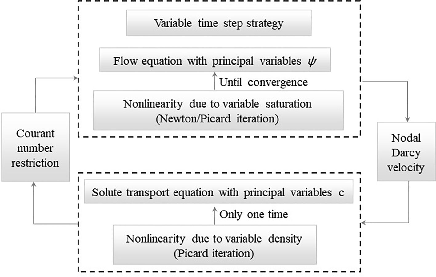
Figure 1 The iteration execution process.

3 Numerical experiments

This study compares the computational properties of the Newton method for solving seawater intrusion problems in three different scenarios after first verifying its accuracy in two conventional cases by the following indices: total CPU time, total iterations, time step size, computation time, iterations head and salinity errors at each time step level $({\Vert {\text{Ψ}}^t-{\text{Ψ}}^{t-\Delta t}\Vert }_{\infty },{\Vert {\text{c}}^t-{\text{c}}^{t-\Delta t}\Vert }_{\infty })$, and submarine groundwater discharge. The application characteristics Newton’s Method for resolving groundwater problems in coastal zones with variable saturations and density-dependent flows were summarised. All the numerical examples in this study were completed using the numerical code MARUN on a workstation Windows 10; and its reliability has been proven for groundwater flow calculations (Boufadel et al., 1999a; Boufadel et al., 1999b; Boufadel et al., 1999c; Li and Boufadel, 2010; Geng and Boufadel, 2015b; Xiao et al., 2019; Yu et al., 2022a; Yu et al., 2023). The MARUN code was developed based on the numerical calculation theory described in Section 2.

When calculating the model, the following conditions were considered: the initial condition was a simple (such as the aquifer is completely saturated and salinity is 0) or complex (according to the MARUN Manual) value; the head convergence standard was set to $\delta$ = 1×10^–5 or 1×10^–10; the grad subdivision size was 0.02 or 0.01 m; the soil hydraulic parameters model (Van Genuchten, 1980) parameters were set to α = 2.0, 5.0, or 40.0 m^–1 and n = 2.0, 4.0 or 7.0; the tides were H_sea = 0.8 + 0.2cos(πt/6), 0.85 + 0.15cos(πt/6), 0.9 + 0.1cos(πt/6), 0.9 + 0.1cos(πt/5), or 0.9 + 0.1cos(πt/4) m; and beach slope were tanθ = 0.1, 0.5, or +∞. The iteration methods used were Newton, Picard, and Newton–Picard (NP), which follows both the Newton and Picard schemes (Putti and Paniconi, 1995):

$\begin{array}{ll}\text{If\hspace{0.17em}}{\Vert {\text{Ψ}}^{n+1,k+1}-{\text{Ψ}}^{n+1,k}\Vert }_{\infty }<{\delta }^{\prime },useEq.(24)& (27)\end{array}$

else use Eq. (25).

where ${\delta }^{\prime }$ denotes the first head convergence tolerance. If the Picard method is slower than the Newton or NP methods, the Newton scheme is deemed effective for the discussion.

3.1 Case validation: typical soil seepage problem and modified Henry problem

Case 1 followed Cooley (1983) and considered a soil freshwater seepage problem in an unsaturated zone, as shown in Figure 2A. The aquifer domain was divided into 2601 nodes and 5000 2 m × 2 m triangle elements. Its steady-state groundwater flow field is shown in Figure 2B. Case 2 referenced (Putti and Paniconi, 1995; Boufadel et al., 1999b) and studied a saline water seepage problem in the saturated zone, as shown in Figure 2C. The aquifer domain was divided into 20301 nodes and 40000 0.01 m × 0.01 m right triangle elements. Its steady-state groundwater flow field is shown in Figure 2D. The hydrogeological parameters are listed in Table 1, and a comparison of the calculation speeds of different methods is shown in Table 2.

FIGURE 2

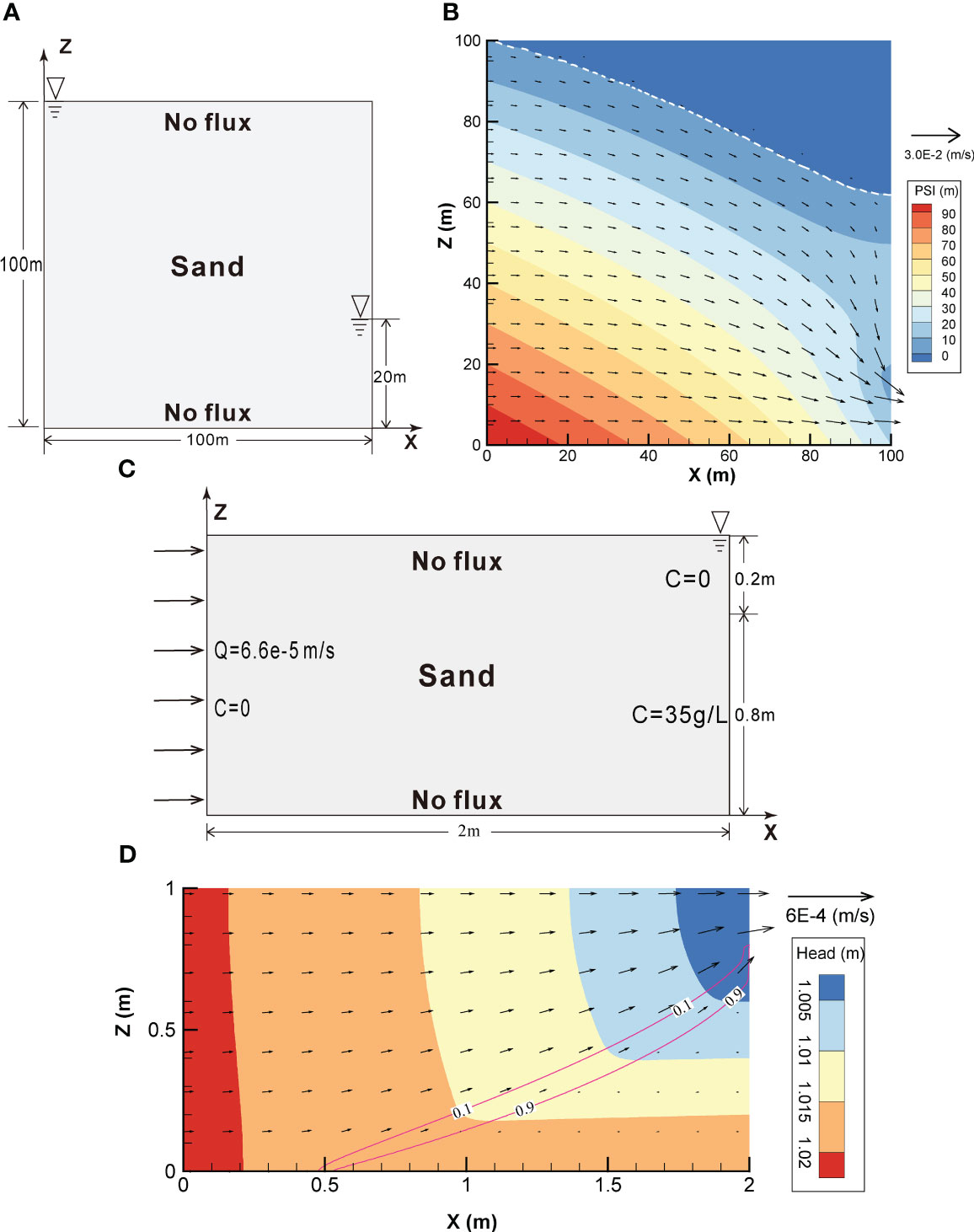
Figure 2 Schematic descriptions of the (A) typical soil seepage and (C) modified Henry problems, and their flow fields, (B) and (D), respectively, following stabilisation. The white dashed line represents the boundary between the saturated and unsaturated zones, while the red solid line represents the contour lines of salinity, as indicated throughout.

TABLE 1

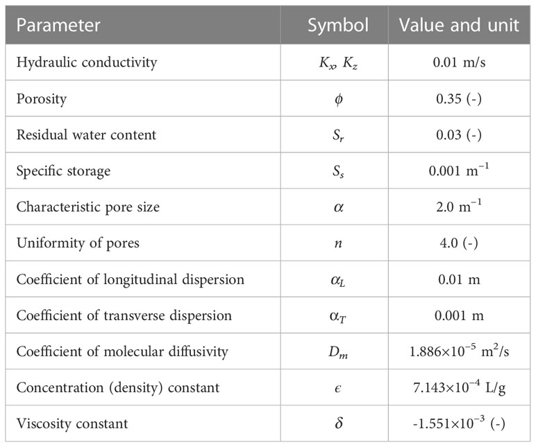
Table 1 Basic hydrogeological parameters of models inspired from (Putti and Paniconi, 1995) and (Boufadel et al., 1999b).

TABLE 2

Table 2 Comparison of the computational speed of Newton methods for solving the typical soil seepage (Cooley, 1983) and modified Henry problems (Putti and Paniconi, 1995; Boufadel et al., 1999b).

The result for Case 1 is the same as that of Cooley (1983). The simulation stabilised in approximately 5 h, and the groundwater was discharged from 20 m below the right boundary. According to Case 1 in Table 2, the CPU time indicated that the calculation speed under complex initial conditions was significantly faster than that under simple initial conditions because the head and salinity were closer to the real value. The calculation speed of the Newton scheme was faster than that of the Picard scheme in any setting, up to 17 times with a head convergence standard of 1×10^–10 and a complex initial value.

In Case 2, seawater was found to have invaded as far as x=0.5m as shown in Figure 2D. After approximately16 h, the simulation reached a steady state. According to Case 2 in Table 2, the CPU time showed that the calculation speed of the coarse mesh generation was significantly faster than that of the fine mesh generation because the size of the nonlinear system decreased with fewer nodes and the calculation amount also decreased. Only when the mesh was finely divided was the Newton scheme 1.23 times faster than the Picard scheme, with a head convergence standard of 10^–10. The model’s overall calculation time increases when salt is involved. The Newton scheme was mainly used to solve the flow equation; if the solution of the solute transport equation cannot improved, the calculation speed cannot be reliably guaranteed.

3.2 Seawater intrusion in unconfined aquifers

In Cases 1 and 2, the benefits of the Newton method for solving variable saturation and density flow models in terms of calculation speed and accuracy were demonstrated. Case 3 referenced to a modified Henry problem. As illustrated in Figure 3A, the right boundary was modified to the Dirichlet boundary of 0.8 m seawater, but the other conditions remained the same. The hydrogeological parameters are listed in Table 1, and the steady state of the groundwater flow field is shown in Figure 3B.

FIGURE 3

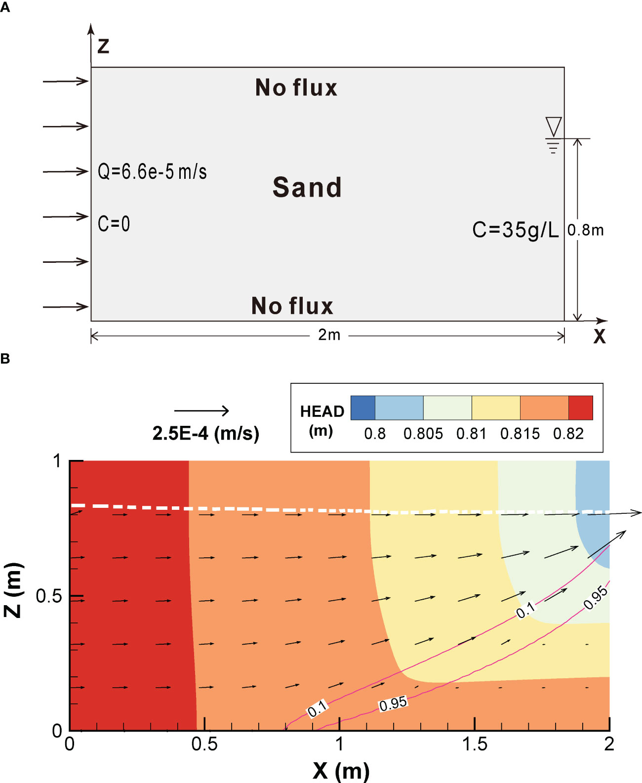
Figure 3 Schematic description of (A) seawater intrusions in unconfined aquifers and the (B) flow field following stabilisation.

The simulated results in Figure 3B show that after mixing with freshwater, seawater is discharged into the ocean from the upper-right boundary, with an intrusion distance of up to 1.2 m. The simulation stabilized after 5 h, generating a salt wedge in the lower-right corner. The entire area had a head distribution ranging from 0.80 to 0.82 m, small hydraulic gradient, slow flow velocity, and a submarine groundwater discharge (SGD) of 5.75×10^–5 m²/s.

Case 3 in Table 3 compares computational speeds of the NP, Picard, and Newton methods for solving various seawater intrusion problems in unconfined aquifers. The calculation speed of the Newton scheme was slightly faster than that of the Picard scheme and was mainly controlled by the soil hydraulic model parameters α and n. Their calculation speeds diverged by more than two times when the soil water distribution in the unsaturated zone was discontinuous. If salinity was included in the model, the calculation of the Newton method would be 1.02 times faster than that of the Picard method. In contrast, the calculation using the Newton method was four times faster than that using the Picard method without salinity. Therefore, salinity slows down the calculation speed of groundwater modelling in an unsaturated zone.

TABLE 3

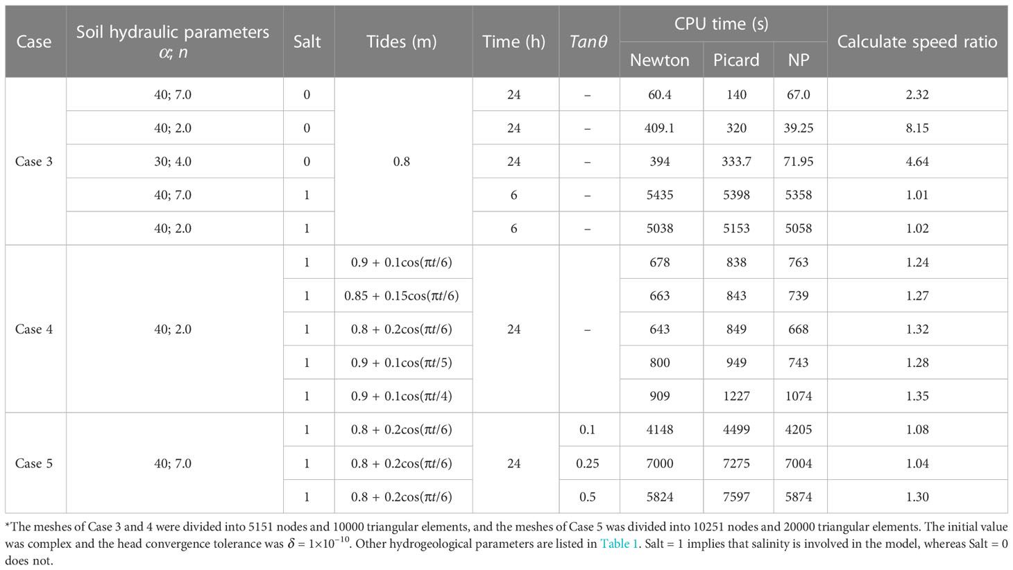
Table 3 Comparison of the computational speeds of Newton methods for solving different seawater intrusion problems.

Figures 4A–C depict the evolution of time step size Δt versus time step level j for several seawater intrusion scenarios simulated using three methods. The time step size Δt was only subjected to the iterations at each time step level in the model without salinity involved. As long as iter< 6, Δt increases until the output control condition is encountered. Generally, the Newton scheme is effective in resolving seawater intrusion in unconfined aquifers. However, it consumes much CPU time to adjust Δt when the initial value is poor. The NP method in this process saves time, as shown in Figures 4A, C. Based on the result with α = 40.0, n = 7.0, the Newton scheme is more dependent on the initial value than the Picard scheme. In the simulation of dry soil wetting, where α = 40.0 and n = 7.0 was direr than α = 40.0 and n = 2.0 and the characteristic curve of moisture content was more nonlinear, the bad initial value failed to reach convergence and induced the oscillation. In this case, the NP method appeared to have greater advantages and could save considerable time during the initial value adjustment process, making it faster than the Picard and Newton methods. However, the calculation speed was completely limited by the Courant number; hence, Δt remained unchanged once salinity was factored into the model, as shown in Figure 4D. Additionally, the total calculation time of the model increased by about 100 times.

FIGURE 4

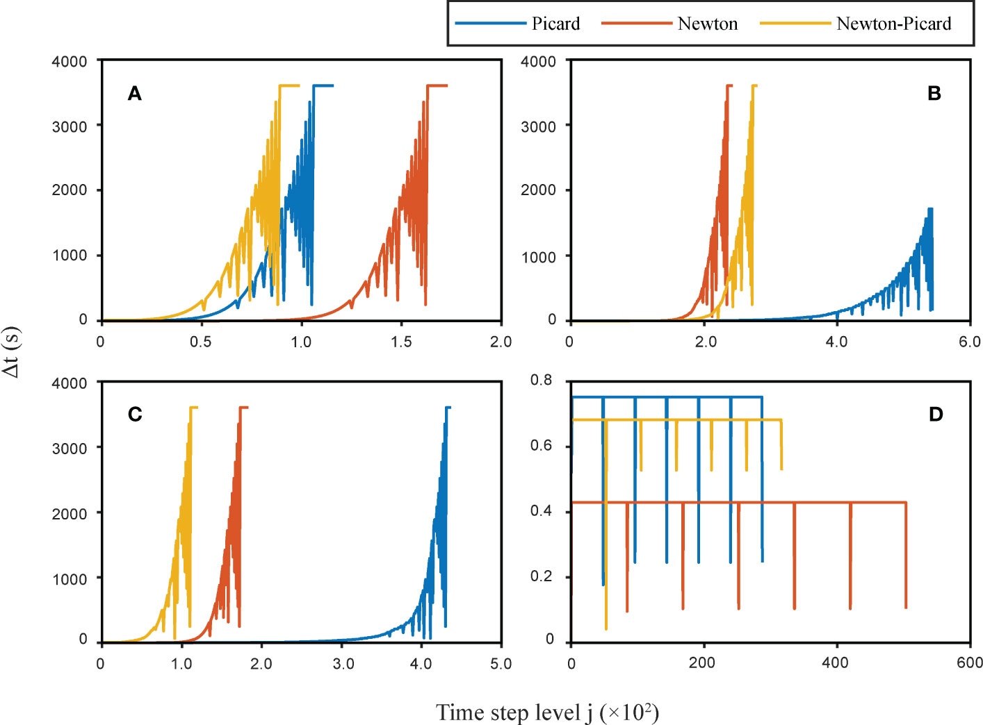
Figure 4 Evolution of time step size Δt versus time step level j for different seawater intrusion scenarios simulated using the Picard, Newton, and NP methods: (A) α = 40.0, n = 2.0, and Salt = 0; (B) α = 40.0, n = 7.0, and Salt = 0; (C) α = 30.0, n = 4.0, and Salt = 0; (D) α = 40.0, n = 2.0, and Salt = 1.

Figure 5 shows the evolution of the head error versus time step level j for different seawater intrusion scenarios simulated using three methods. In Figure 5A, the Newton and NP methods both converge to 10^–15, while the Picard method only converges to 10^–12. The convergence speed of the Newton and NP methods was higher than that of the Picard methods for α = 40.0 and n = 7.0, and α = 30.0 and n = 4.0, as shown in Figures 5B, C. Based on this, the Newton scheme is more convergent than the Picard scheme in certain cases.

FIGURE 5

Figure 5 Evolution of head error ${\Vert {\text{Ψ}}^{n+1}-{\text{Ψ}}^{n+1}\Vert }_{\infty }$ versus time step level j for different seawater intrusion scenarios simulated using the Picard, Newton, and NP methods: (A) α = 40.0 and n = 2.0; (B) α = 40.0 and n = 7.0; (C) α = 30.0 and n = 4.0; (D) α = 40.0, n = 2.0, and Salt = 1.

3.3 Seawater intrusion by tidal action

According to previous studies (Li et al., 2008; Li and Boufadel, 2010; Geng et al., 2015; Geng et al., 2016; Xiao et al., 2017; Yu et al., 2022b), tides are a major factor affecting groundwater flow and solute transport in coastal zones. Based on Case 4 (Figure 6A),the right boundary is the set of tides of varying amplitudes and frequencies. The hydrogeological parameters are provided in Table 1, and the average groundwater flow field diagram for one tidal period following stabilisation is shown in Figure 6B. The groundwater flow fields at the high tide and low tide levels are shown in Figures 6C, D, respectively.

FIGURE 6

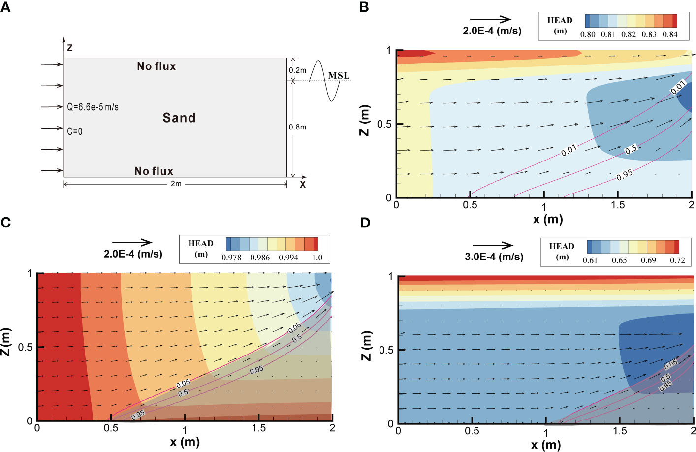
Figure 6 Schematic descriptions of a (A) seawater intrusion tide, 0.8 + 0.2cos(πt/6); the (B) average groundwater flow field of one tidal period following stabilization; the (C, D) groundwater flow fields at high tide and low tide levels.

As shown in Figure 6B, the seawater intrusion distance reached up to 1.52 m. The entire area has a head distribution ranging from 0.80 to 0.84 m, a large hydraulic gradient, a fast flow velocity, and an SGD of 5.75 × 10^–5 m²/s. The seawater invaded zone (i.e., the shadow part) gradually shrank with the tide level dropping as shown in Figures 6C, D. Case 4 in Table 3 compares of the computational speeds of the NP, Picard, and Newton methods for solving seawater intrusion with different tides. The higher the tidal frequency, the stronger the hydrodynamic conditions in an unsaturated soil zone, leading to a more complex microscopic pore flow. Additionally, a larger tidal amplitude results in a larger unsaturated zone. As a consequence, the Newton scheme offers more noticeable advantages in terms of calculation speed. For instance, when the tidal frequency rises from π/6 and π/5 to π/4, the calculated speed ratio changes from 1.24 and 1.28 to 1.35, respectively. And the calculated speed ratio changes from 1.24 and 1.27 to 1.32 as the tidal amplitude increases from 0.1 and 0.15 to 0.2 m, respectively.

Furthermore, as the tidal amplitude and frequency increased, more triangular elements alternating between wet and dry states were exposed in the near-surface unsaturated zone, increasing computation time for the entire model. Due to the salinity involved in the model, Δt was limited by the Courant number and was maintained at a constant value at different time step levels. This is similar to Figure 5D; therefore, it is not shown here. If the iterations at different time steps are the same, the calculation speed of the Newton (or NP) method may be lower than that of the Picard method because of the high CPU consumption of the Newton scheme.

The evolution of the head and salinity errors versus time step level j using the Picard, Newton, and NP methods is essentially the same, as shown in Figure 7. The relative errors of the head or salt were the largest around the middle tidal line, where the water level changes most sharply, and the least near the high and low tidal lines, where the water level varies most slowly. That is, the error increases and then decreases during ebb and high tides, respectively. Moreover, a bigger frequency and amplitude will account for more head and salinity inaccuracies, that is, 10^–5< ψ_error< × 10^–3, 5.3 × 10^–2< c_error< 1.9 when H_sea= 0.9 + 0.1cos(πt/6), but 10^–5< ψ_error< 10^–2, 0.2< c_error< 19.9 when H_sea= 0.8 + 0.2cos(2πt).

FIGURE 7

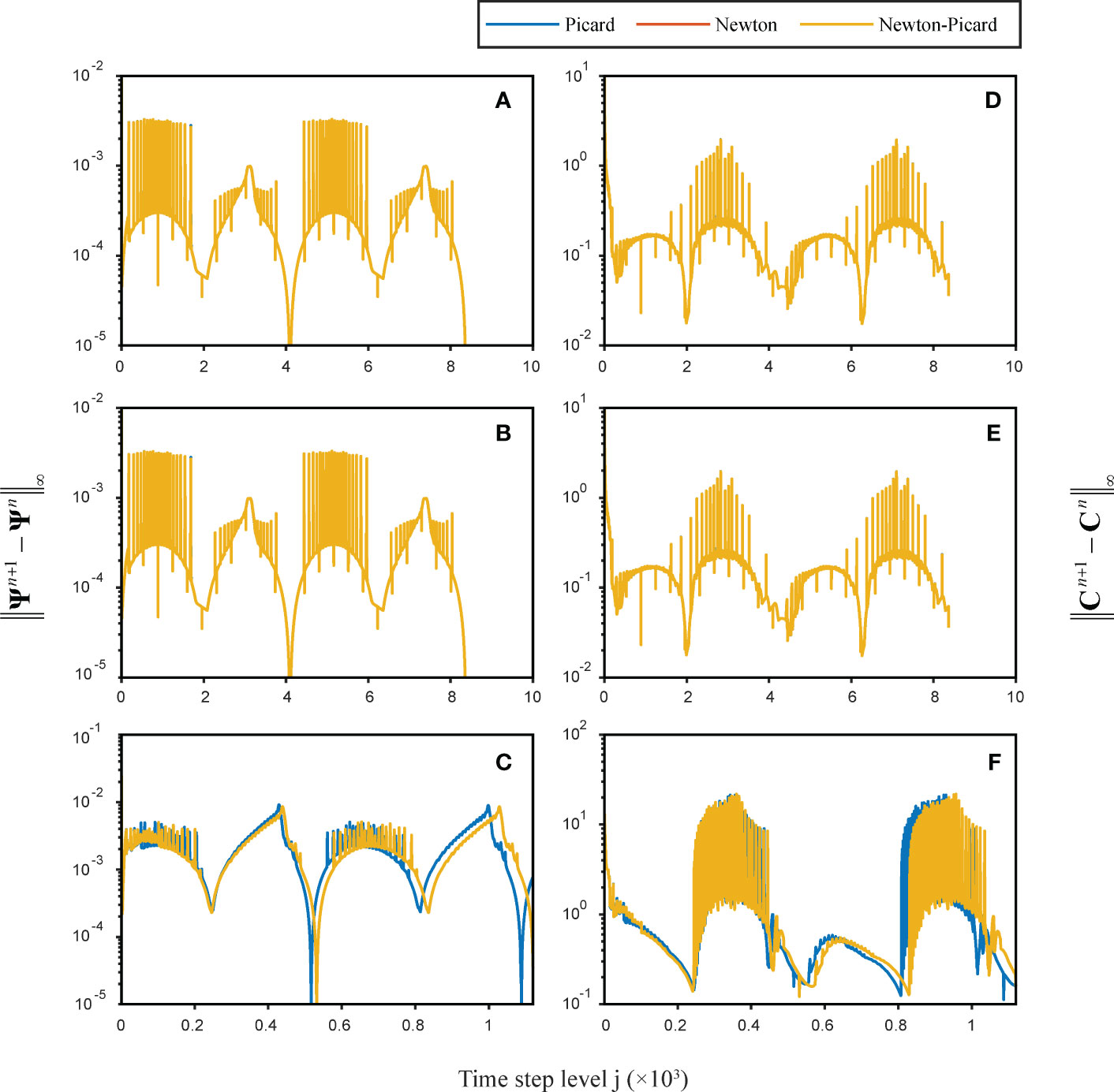
Figure 7 Evolution of head and salinity errors versus time step level j of different seawater intrusion scenarios simulated using the Picard, Newton and NP methods. (A, D) H_sea = 0.8 + 0.2cos(πt/6); (B, E) H_sea = 0.9 + 0.1cos(πt/6); (C, F) H_sea = 0.8 + 0.2cos(2πt).

3.4 Seawater intrusion on a slope beach

The surfaces of coastal aquifers typically feature a slope that can alter the paths of porewater and effectively prevent seawater intrusion (Li et al., 2008). Here, a sloped and narrow intertidal zone (tanθ = 0.1) on the upper surface was consideration on the basis of Section 3.3, as shown in Figure 8A. The hydrogeological parameters are listed in Table 1, and the average groundwater flow field diagram for one tidal period cycle following stabilisation is shown in Figure 8B. The groundwater flow field at the high tide and low tide levels is shown in Figures 8C, D, respectively.

FIGURE 8

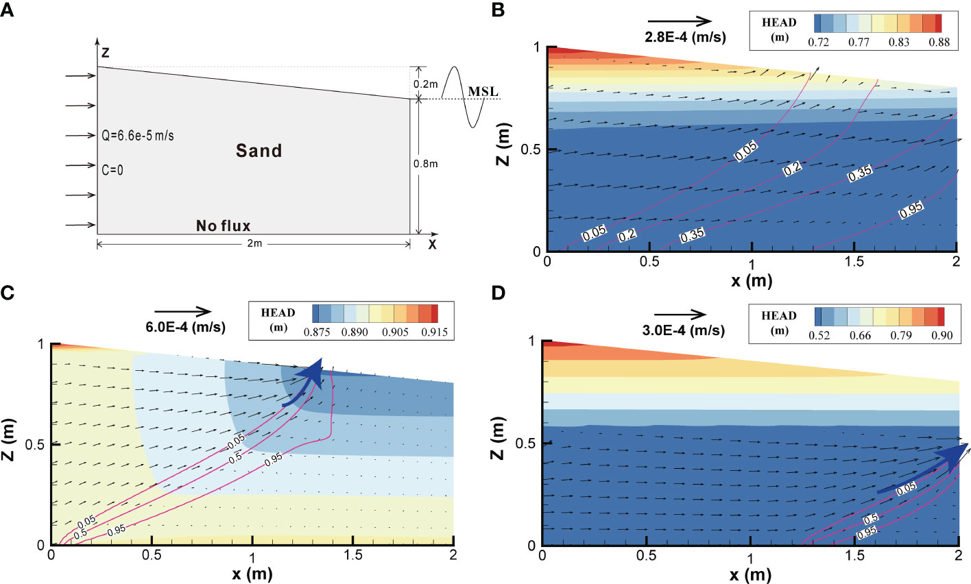
Figure 8 Schematic descriptions of (A) seawater intrusion with a sloping aquifer; the (B) average groundwater flow field of one tidal period cycle following stabilisation; the (C, D) groundwater flow fields at high tide and low tide levels.

The seawater intrusion distance was up 1.94 m and the entire area had a head distribution ranging from 0.72 to 0.88 m, as shown in Figure 8B. As the hydraulic gradient increased, the flow velocity also increased with an SGD of 3.53 × 10^–5 m²/s. Figures 8C, D show that the freshwater discharge ports (the blue arrows) moved down with the seawater level. Case 5 in Table 3 compares the computational speed of NP, Picard and Newton methods for solving seawater intrusion with a sloping aquifer. The slope of the aquifer and the total CPU time of the Picard method were smaller. The greater the aquifer slope, the greater the hydraulic gradient, and the faster the groundwater flow, which results in a smaller time step size based on the Courant number and a slower overall computation. Furthermore, the Newton scheme offer the most obvious advantages for the terrain with the largest slope. The more triangular elements alternate between wet and dry conditions and are exposed in the near-surface unsaturated zone caused by tidal fluctuations, the worse the continuity of pore flow affected by topography, and the longer the water retention time.

Figure 9 shows the evolution of different factors versus the time step level j of the seawater intrusion problem with a sloping aquifer simulated using three methods. Although the iterations at each time step level were always fewer than six times in Figure 9A, the time step size of the three methods was always bounded to 2 s by the Courant number, as shown in Figure 9B. The computation time at each time step level of the Picard scheme was greater than that of the Newton scheme (Figure 9C); therefore, the total CPU time of the Picard method was approximately 3000 s less than that of the Newton method, as shown in Figure 9D. The head and salinity calculation errors for the seawater intrusion problem with a sloping aquifer were simulated using different methods. The evolution of head and salinity errors versus time step level j showed periodic changes with the ebb and flow of the sea tide, which are essentially consistent with those in Section 3.3 and are not shown here.

FIGURE 9

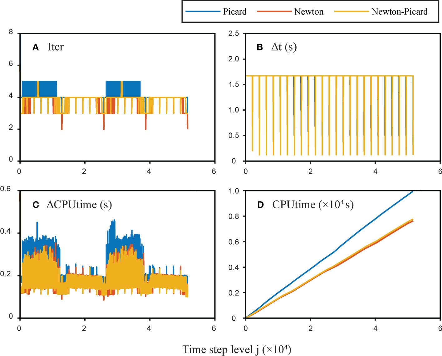
Figure 9 Evolutions of different factors versus time step level j of the seawater intrusion problem with a sloping aquifer simulated using the Picard, Newton, and NP methods: (A) iterations at each time step level; (B) time step size Δt; (C) CPU time at each time step level; and (D) sum of CPU time until current time step level.

4 Summary and discussion

The coupled system of groundwater flow and solute transport in coastal aquifer with variable saturation and density contains several nonlinear terms, that can only be resolved using numerical methods. Numerical methods for solving such large-scale nonlinear problems must employ an efficient (ensuring the optimal utilisation of CPU and storage resources to achieve the desired accuracy of the solution) and robust (showing acceptable convergence in a wide range of simulation scenarios) algorithm.

Although the Newton iterative scheme have been applied to solve a series of groundwater flow problems in porous media with variable saturation, including 1D, 2D, and 3D steady and unsteady flows, these did not consider the influence of many nonlinear factors special to the coastal zone on the Newton iterative calculation. This study presented the finite element numerical discrete form of groundwater flow and solute transport equation in the coastal zone, the Picard and Newton iterative framework, and a new numerical solution. The reliability of the numerical solution was demonstrated by resolving a typical soil water seepage problem and a modified Henry problem. This was then applied to three different scenarios to solve the seawater intrusion problem.

The computational advantages and disadvantages of different solutions are compared, which revealed that several factors affect the speed of solving the problem of coastal groundwater flow, including the initial values of the model, the soil hydraulic model, tidal changes, slope effects, and the size of the grid. Tidal action represents the strong hydrological conditions at the surface, while slope effects and soil hydraulic model represent the hydraulic characteristics of the aquifer. These factors first affect the groundwater flow and solute transport processes in the shallow aquifer, especially in the unsaturated soil zone, thereby affecting the nonlinearity of the flow equation and ultimately affecting the speed of model calculation. The size of the grid directly determines the order of the equation group after numerical discretisation. The higher the order, the greater the required hardware storage and computational resources, directly affecting the model calculation time. Once the model considers salinity, the calculation speed will be limited by the Courant number, which directly affects the model’s calculation time. Finally, the initial values directly determine the convergence speed of the equation group, and also play a key role in determining whether the Newton-Picard method can outperform the Picard method. A single iteration calculation of the Newton method takes more time than the Picard method, making it necessary to use fewer iterations than the Picard method to exchange for a greater computational advantage.

If the grid is relatively coarse (the order of the nonlinear matrix equation is lower) and the soil hydraulic model parameters α is large and n is small (the nonlinearity of the flow equation increases), then the Newton scheme has higher convergence accuracy and faster computational speed than the Picard scheme. In case 2, the computational speed of the Newton method can be as fast as 17 times that of the Picard method. In case 1, the computational accuracy of the Newton method is three orders of magnitude higher than that of the Picard method.

If the frequency and amplitude of the sea level fluctuation are high and the slope of the aquifer is steep, the local flow in the unsaturated zone becomes more complex, and the computational advantage of the Newton method is present. In Cases 4 and 5, the computational speed of the Newton iteration scheme can reach about 1.3 times that of the Picard scheme (e.g., the tidal wave amplitude increases to 0.3 m, the tidal wave frequency is 6.28 rad/h, or the slope of the tilted beach is tanθ = 0.5).

Overall, compared with the classical Picard scheme, the Newton scheme has advantages in computing speed and better convergence, but it increases the hardware cost of the computer. Therefore, additional optimisation methods should be considered during the actual calculation process, and multiple simulations should be attempted to determine the most effective numerical algorithm for different problems.

5 Conclusions

In this study, a new derived numerical solution of the coastal groundwater flow problem based on the Newton scheme was constructed, and the FORTRAN codes of the Newton and NP methods were written for the use of the relevant personnel. Their calculation effects in solving different numerical models (including two typical cases and three seawater intrusion models) were compared and analyzed. The following conclusions were drawn:

i. The variable-density effect caused by salinity significantly slowed the overall calculation of the model, but the main reason for the great difference in calculation speed of different solutions is still the variable saturation.

ii. The calculation speed of the Newton scheme is influenced by the initial value, soil hydrodynamic model parameters, tidal fluctuations, and slope effect. If the frequency and amplitude of the tidal fluctuations is larger, the slope of the aquifer is larger, and the soil hydraulic model parameter α is larger and n is smaller, the local flow in unsaturated zone will be more complex, and the nonlinear flow equation will be stronger. Compared with the Picard scheme, the Newton scheme has higher convergence accuracy and faster calculation speed.

iii. Among Newton, Picard and NP methods, the NP method can improve the robustness of the solution and overcome the sensitivity of the solution process to the initial value estimation compared with the Newton method. The NP method optimizes the convergence of the solution and can achieve higher convergence accuracy through fewer iterations under the condition of relatively appropriate initial values in compared with the Picard method.

Data availability statement

The datasets presented in this study can be found in online repositories. The names of the repository/repositories and accession number(s) can be found below: https://github.com/yaomeng-sustech/Newton-Iteration.

Author contributions

MY designed the study, finished the coding and wrote the original draft preparation. SY contributed to the manuscript writing and programming. HL contributed to the study design, revised the manuscript and acquired funding. All authors contributed to the article and approved the submitted version.

Funding

This work was supported by the Key Program of National Natural Science Foundation of China (Grant No. 42130703), the Shenzhen Science and Technology Innovation Committee (Grant No. JCYJ20200925174525002), and National Natural Science Foundation of China (Grant No. 41972260).

Acknowledgments

The calculations were performed on the Taiyi high-performance supercomputer cluster, support by Center for Computational Science and Engineering at Southern University of Science and Technology.

Conflict of interest

The authors declare that the research was conducted in the absence of any commercial or financial relationships that could be construed as a potential conflict of interest.

Publisher’s note

All claims expressed in this article are solely those of the authors and do not necessarily represent those of their affiliated organizations, or those of the publisher, the editors and the reviewers. Any product that may be evaluated in this article, or claim that may be made by its manufacturer, is not guaranteed or endorsed by the publisher.

References

Abdollahi-Nasab A., Boufadel M. C., Li H., Weaver J. W. (2010). Saltwater flushing by freshwater in a laboratory beach. J. Hydrol. 386 (1-4), 1–12. doi: 10.1016/j.jhydrol.2009.12.005

CrossRef Full Text | Google Scholar

America I., Zhang C., Werner A. D., van der Zee S.E.A.T.M. (2020). Evaporation and salt accumulation effects on riparian freshwater lenses. Water Resour. Res. 56 (12), e2019WR026380. doi: 10.1029/2019WR026380

CrossRef Full Text | Google Scholar

Bergamaschi L., Putti M. (1999). Mixed finite elements and newton-type linearizations for the solution of richards' equation. Int. J. numerical Methods Eng. 45 (8), 1025–1046. doi: 10.1002/(SICI)1097-0207(19990720)45:8<1025::AID-NME615>3.0.CO;2-G

CrossRef Full Text | Google Scholar

Boufadel M., Geng X., An C., Owens E., Chen Z., Lee K., et al. (2019). A review on the factors affecting the deposition, retention, and biodegradation of oil stranded on beaches and guidelines for designing laboratory experiments. Curr. pollut. Rep. 5 (4), 407–423. doi: 10.1007/s40726-019-00129-0

CrossRef Full Text | Google Scholar

Boufadel M., Suidan M., Venosa A. (1999a). Numerical modeling of water flow below dry salt lakes: effect of capillarity and viscosity. J. Hydrol. 221 (1-2), 55–74. doi: 10.1016/S0022-1694(99)00077-3

CrossRef Full Text | Google Scholar

Boufadel M. C., Suidan M. T., Venosa A. D. (1999b). A numerical model for density-and-viscosity-dependent flows in two-dimensional variably saturated porous media. J. Contaminant Hydrol. 37 (1-2), 1–20. doi: 10.1016/S0169-7722(98)00164-8

CrossRef Full Text | Google Scholar

Boufadel M. C., Suidan M. T., Venosa A. D., Bowers M. T. (1999c). Steady seepage in trenches and dams: effect of capillary flow. J. Hydraulic Eng. 125 (3), 286–294. doi: 10.1061/(ASCE)0733-9429(1999)125:3(286

CrossRef Full Text | Google Scholar

Boufadel M. C., Xia Y., Li H. (2011). Modeling solute transport and transient seepage in a laboratory beach under tidal influence. Environ. Model. Softw. 26 (7), 899–912. doi: 10.1016/j.envsoft.2011.02.005

CrossRef Full Text | Google Scholar

Celia M. A., Bouloutas E. T., Zarba R. L. (1990). A general mass-conservative numerical solution for the unsaturated flow equation. Water Resour. Res. 26 (7), 1483–1496. doi: 10.1029/WR026i007p01483

CrossRef Full Text | Google Scholar

Choo J. (2018). Large Deformation poromechanics with local mass conservation: an enriched galerkin finite element framework. Int. J. Numerical Methods Eng. 116 (1), 66–90. doi: 10.1002/nme.5915

CrossRef Full Text | Google Scholar

Cooley R. L. (1983). Some new procedures for numerical solution of variably saturated flow problems. Water Resour. Res. 19 (5), 1271–1285. doi: 10.1029/WR019i005p01271

CrossRef Full Text | Google Scholar

D'Haese C. M. F., Putti M., Paniconi C., Verhoest N. E. C. (2007). Assessment of adaptive and heuristic time stepping for variably saturated flow. Int. J. Numerical Methods Fluids 53 (7), 1173–1193. doi: 10.1002/fld.1369

CrossRef Full Text | Google Scholar

Geng X., Boufadel M. C. (2015a). Impacts of evaporation on subsurface flow and salt accumulation in a tidally influenced beach. Water Resour. Res. 51 (7), 5547–5565. doi: 10.1002/2015WR016886

CrossRef Full Text | Google Scholar

Geng X., Boufadel M. C. (2015b). Numerical study of solute transport in shallow beach aquifers subjected to waves and tides. J. Geophys. Res.: Oceans 120 (2), 1409–1428. doi: 10.1002/2014JC010539

CrossRef Full Text | Google Scholar

Geng X., Boufadel M. C. (2017). The influence of evaporation and rainfall on supratidal groundwater dynamics and salinity structure in a sandy beach. Water Resour. Res. 53 (7), 6218–6238. doi: 10.1002/2016WR020344

CrossRef Full Text | Google Scholar

Geng X., Boufadel M. C., Lee K., Abrams S., Suidan M. (2015). Biodegradation of subsurface oil in a tidally influenced sand beach: impact of hydraulics and interaction with pore water chemistry. Water Resour. Res. 51 (5), 3193–3218. doi: 10.1002/2014WR016870

CrossRef Full Text | Google Scholar

Geng X., Boufadel M. C., Xia Y., Li H., Zhao L., Jackson N. L., et al. (2014). Numerical study of wave effects on groundwater flow and solute transport in a laboratory beach. J. contam. hydrol. 165, 37–52. doi: 10.1016/j.jconhyd.2014.07.001

PubMed Abstract | CrossRef Full Text | Google Scholar

Geng X., Pan Z., Boufadel M. C., Ozgokmen T., Lee K., Zhao L. (2016). Simulation of oil bioremediation in a tidally influenced beach: spatiotemporal evolution of nutrient and dissolved oxygen. J. Geophys. Res.: Oceans 121 (4), 2385–2404. doi: 10.1002/2015JC011221

CrossRef Full Text | Google Scholar

Guo Q., Li H., Zhou Z., Huang Y. (2012). Rainfall infiltration-derived submarine groundwater discharge from multi-layered aquifer system terminating at the coastline. Hydrol. Processes 26 (7), 985–995. doi: 10.1002/hyp.8188

CrossRef Full Text | Google Scholar

Hou Y., Yang J., Russoniello C. J., Zheng T., Wu M.-l., Yu X. (2022). Impacts of coastal shrimp ponds on saltwater intrusion and submarine groundwater discharge. Water Resour. Res. 58 (7), e2021WR031866. doi: 10.1029/2021WR031866

CrossRef Full Text | Google Scholar

Huang K., Mohanty B. P., Leij F. J., van Genuchten M. T. (1998). Solution of the nonlinear transport equation using modified picard iteration. Adv. Water Resour. 21 (3), 237–249. doi: 10.1016/S0309-1708(96)00046-2

CrossRef Full Text | Google Scholar

Huang K., Mohanty B., Van Genuchten M. T. (1996). A new convergence criterion for the modified picard iteration method to solve the variably saturated flow equation. J. Hydrol. 178 (1-4), 69–91. doi: 10.1016/0022-1694(95)02799-8

CrossRef Full Text | Google Scholar

Huyakorn P. S. (2012). Computational methods in subsurface flow (Reston: Academic Press).

Google Scholar

Huyakorn P. S., Springer E. P., Guvanasen V., Wadsworth T. D. (1986). A three-dimensional finite-element model for simulating water flow in variably saturated porous media. Water Resour. Res. 22 (13), 1790–1808. doi: 10.1029/WR022i013p01790

CrossRef Full Text | Google Scholar

Huyakorn P. S., Thomas S. D., Thompson B. M. (1984). Techniques for making finite elements competitve in modeling flow in variably saturated porous media. Water Resour. Res. 20 (8), 1099–1115. doi: 10.1029/WR020i008p01099

CrossRef Full Text | Google Scholar

Istok J. (1989). Groundwater modeling by the finite element method. Water Resour. monograph. 13, 176–225. doi: 10.1029/WM013

CrossRef Full Text | Google Scholar

Kavetski D., Binning P., Sloan S. W. (2002). Adaptive backward Euler time stepping with truncation error control for numerical modelling of unsaturated fluid flow. Int. J. Numerical Methods Eng. 53 (6), 1301–1322. doi: 10.1002/nme.329

CrossRef Full Text | Google Scholar

Kees C. E., Farthing M. W., Dawson C. N. (2008). Locally conservative, stabilized finite element methods for variably saturated flow. Comput. Methods Appl. Mechanics Eng. 197 (51), 4610–4625. doi: 10.1016/j.cma.2008.06.005

CrossRef Full Text | Google Scholar

Li H., Boufadel M. C. (2010). Long-term persistence of oil from the Exxon Valdez spill in two-layer beaches. Nat. Geosci. 3 (2), 96–99. doi: 10.1038/ngeo749

CrossRef Full Text | Google Scholar

Li H., Boufadel M. C., Weaver J. W. (2008). Tide-induced seawater–groundwater circulation in shallow beach aquifers. J. Hydrol. 352 (1-2), 211–224. doi: 10.1016/j.jhydrol.2008.01.013

CrossRef Full Text | Google Scholar

Liu Y., Kuang X., Jiao J. J., Li J. (2015). Numerical study of variable-density flow and transport in unsaturated–saturated porous media. J. Contaminant Hydrol. 182, 117–130. doi: 10.1016/j.jconhyd.2015.09.001

CrossRef Full Text | Google Scholar

Lott P., Walker H., Woodward C., Yang U. (2012). An accelerated picard method for nonlinear systems related to variably saturated flow. Adv. Water Resour. 38, 92–101. doi: 10.1016/j.envpol.2022.119572

CrossRef Full Text | Google Scholar

Mehl S. (2006). Use of picard and newton iteration for solving nonlinear ground water flow equations. Groundwater 44 (4), 583–594. doi: 10.1111/j.1745-6584.2006.00207.x

CrossRef Full Text | Google Scholar

Najem W. (1982). Introduction aux techniques du calcul numerique in French. (Beirut, Lebanon: Engineering Faculty, University of Saint Joseph), 54.

Google Scholar

Neuman S. P. (1973). Saturated-unsaturated seepage by finite elements. J. hydraulics division 99 (12), 2233–2250. doi: 10.1061/JYCEAJ.0003829

CrossRef Full Text | Google Scholar

Norambuena-Contreras J., Arbat G., García Nieto P. J., Castro-Fresno D. (2012). Nonlinear numerical simulation of rainwater infiltration through road embankments by FEM. Appl. Math. Comput. 219 (4), 1843–1852. doi: 10.1016/j.amc.2012.08.025

CrossRef Full Text | Google Scholar

Paniconi C., Putti M. (1994). A comparison of picard and newton iteration in the numerical solution of multidimensional variably saturated flow problems. Water Resour. Res. 30 (12), 3357–3374. doi: 10.1029/94WR02046

CrossRef Full Text | Google Scholar

Peters A., Durner W. (2008). Simplified evaporation method for determining soil hydraulic properties. J. Hydrol. 356 (1), 147–162. doi: 10.1016/j.jhydrol.2008.04.016

CrossRef Full Text | Google Scholar

Philip J. (1957). The theory of infiltration: 1. the infiltration equation and its solution. Soil Sci. 83 (5), 345–358. doi: 10.1097/00010694-195705000-00002

CrossRef Full Text | Google Scholar

Putti M., Paniconi C. (1995). Picard and newton linearization for the coupled model for saltwater intrusion in aquifers. Adv. Water Resour. 18 (3), 159–170. doi: 10.1016/0309-1708(95)00006-5

CrossRef Full Text | Google Scholar

Qu W., Li H., Wan L., Wang X., Jiang X. (2014). Numerical simulations of steady-state salinity distribution and submarine groundwater discharges in homogeneous anisotropic coastal aquifers. Adv. Water Resour. 74, 318–328. doi: 10.1016/j.advwatres.2014.10.009

CrossRef Full Text | Google Scholar

Shao C., Guan Y., Chu C., Shi R., Ju M., Shi J. (2014). Trends analysis of ecological environment security based on DPSIR model in the coastal zone: a survey study in tianjin, China. Int. J. Environ. Res. 8 (3), 765–778. doi: 10.22059/IJER.2014.770

CrossRef Full Text | Google Scholar

Simmons C. T., Pierini M. L., Hutson J. L. (2002). Laboratory investigation of variable-density flow and solute transport in unsaturated–saturated porous media. Transport Porous Media 47 (2), 215–244. doi: 10.1023/A:1015568724369

CrossRef Full Text | Google Scholar

Singh S., Raju N. J., Gossel W., Wycisk P. (2016b). Assessment of pollution potential of leachate from the municipal solid waste disposal site and its impact on groundwater quality, varanasi environs, India. Arabian J. Geoscie. 9 (2), 131. doi: 10.1007/s12517-015-2131-x

CrossRef Full Text | Google Scholar

Singh M., Singh C., Gangacharyulu D. (2016a). Modeling for flow through unsaturated porous media with constant and variable density conditions using local thermal equilibrium. Int. J. Comput. Appl. 5, 24–30.

Google Scholar

Su D., Mayer K. U., MacQuarrie K. T. B. (2020). Numerical investigation of flow instabilities using fully unstructured discretization for variably saturated flow problems. Adv. Water Resour. 143, 103673. doi: 10.1016/j.advwatres.2020.103673

CrossRef Full Text | Google Scholar

Tartakovsky A. M., Marrero C. O., Perdikaris P., Tartakovsky G. D., Barajas-Solano D. (2020). Physics-informed deep neural networks for learning parameters and constitutive relationships in subsurface flow problems. Water Resour. Res. 56 (5), e2019WR026731. doi: 10.1029/2019WR026731

CrossRef Full Text | Google Scholar

Van Genuchten M. T. (1980). A closed-form equation for predicting the hydraulic conductivity of unsaturated soils. Soil Sci. Soc. America J. 44 (5), 892–898. doi: 10.2136/sssaj1980.03615995004400050002x

CrossRef Full Text | Google Scholar

Voss C. I. (1984). A finite-element simulation model for saturated-unsaturated, fluid-density-dependent ground-water flow with energy transport or chemically-reactive single-species solute transport. Water Resour. Invest. Rep. 84, 4369. doi: 10.3133/wri844369

CrossRef Full Text | Google Scholar

Wang W., Dai Z., Li J., Zhou L. (2012). A hybrid Laplace transform finite analytic method for solving transport problems with large peclet and courant numbers. Comput. Geoscie. 49, 182–189. doi: 10.1016/j.cageo.2012.05.020

CrossRef Full Text | Google Scholar

Xiao K., Li H., Wilson A. M., Xia Y., Wan L., Zheng C., et al. (2017). Tidal groundwater flow and its ecological effects in a brackish marsh at the mouth of a large sub-tropical river. J. Hydrol. 555, 198–212. doi: 10.1016/j.jhydrol.2017.10.025

CrossRef Full Text | Google Scholar

Xiao K., Li H., Xia Y., Yang J., Wilson A. M., Michael H. A., et al. (2019). Effects of tidally varying salinity on groundwater flow and solute transport: insights from modelling an idealized creek marsh aquifer. Water Resour. Res. 55 (11), 9656–9672. doi: 10.1029/2018WR024671

CrossRef Full Text | Google Scholar

Younes A., Koohbor B., Belfort B., Ackerer P., Doummar J., Fahs M. (2022). Modeling variable-density flow in saturated-unsaturated porous media: an advanced numerical model. Adv. Water Resour. 159, 104077. doi: 10.1016/j.advwatres.2021.104077

CrossRef Full Text | Google Scholar

Yu S., Jiao J. J., Luo X., Li H., Wang X., Zhang X., et al. (2023). Evolutionary history of the groundwater system in the pearl river delta (China) during the Holocene. Geology 51 (5), 481–485. doi: 10.1130/G50888.1

CrossRef Full Text | Google Scholar

Yu S., Wang C., Li H., Zhang X., Wang X., Qu W. (2022a). Field and numerical investigations of wave effects on groundwater flow and salt transport in a sandy beach. Water Resour. Res. 58 (11), e2022WR032077. doi: 10.1029/2022WR032077

CrossRef Full Text | Google Scholar

Yu S., Zhang X., Li H., Wang X., Wang C., Kuang X. (2022b). Analytical study for wave-induced submarine groundwater discharge in subtidal zone. J. Hydrol. 612, 128219. doi: 10.1016/j.jhydrol.2022.128219

CrossRef Full Text | Google Scholar

Zha Y., Yang J., Yin L., Zhang Y., Zeng W., Shi L. (2017). A modified picard iteration scheme for overcoming numerical difficulties of simulating infiltration into dry soil. J. hydrol. 551, 56–69. doi: 10.1016/j.jhydrol.2017.05.053

CrossRef Full Text | Google Scholar

Zhang Z., Wang W., Gong C., Yeh T.-c., Duan L., Wang Z. (2021). Finite analytic method: analysis of one-dimensional vertical unsaturated flow in layered soils. J. Hydrol. 597, 125716. doi: 10.1016/j.jhydrol.2020.125716

CrossRef Full Text | Google Scholar